Dynamic Combination of Heterogeneous Models for
Hierarchical Time Series

Abstract

We introduce a framework to dynamically combine heterogeneous models called DYCHEM, which forecasts a set of time series that are related through an aggregation hierarchy. Different types of forecasting models can be employed as individual “experts” so that each model is tailored to the nature of the corresponding time series. DYCHEM learns hierarchical structures during the training stage to help generalize better across all the time series being modeled and also mitigates coherency issues that arise due to constraints imposed by the hierarchy. To improve the reliability of forecasts, we construct quantile estimations based on the point forecasts obtained from combined heterogeneous models. The resulting quantile forecasts are coherent and independent of the choice of forecasting models. We conduct a comprehensive evaluation of both point and quantile forecasts for hierarchical time series (HTS), including public data and user records from a large financial software company. In general, our method is robust, adaptive to datasets with different properties, and highly configurable and efficient for large-scale forecasting pipelines.

I Introduction

Forecasting time-series with hierarchical aggregation constraints is a common problem in many practically important applications [12, 15, 20, 33, 39]. For example, retail sales and inventory records are normally at different granularities such as product categories, store, city and state [22, 27]. Generating forecasts for each aggregation level is necessary in developing both high-level and detailed view of marketing insights. Another prominent example is population forecast at multiple time granularities such as monthly, quarterly, and yearly basis [2]. Normally, data at different aggregation levels possess distinct properties w.r.t. sparsity, noise distribution, sampling frequency etc. A well-generalized forecasting model should not only forecast each time series independently, but also exhibit coherency across the hierarchy. However, generating forecasts using regular multivariate forecasting models does not lead to forecasts that satisfy the coherency requirement.

A major group of works for HTS forecasting employ a two-stage (or post-training) approach [3, 12, 15, 37], where base forecasts are firstly obtained for each time series followed by a reconciliation among these forecasts. The reconciliation step involves computing a weight matrix $P$ taking into account the hierarchy, which linearly maps the base forecasts to coherent results. This approach guarantees coherent results but relies on strong assumptions (Gaussian error assumption; [12, 15, 37] also require unbiased base forecast assumption). Moreover, computing $P$ is expensive because of matrix inversion, making this method unsuitable for large-scale forecasting pipelines. Another line of work attempts to learn inter-level relationships during the model training stage. [11] provides a controllable trade-off between forecasting accuracy of single time series and coherency across the hierarchy, which connects reconciliation with learned parameters of forecasting models. However, one needs to modify the objective functions of the individual models, which is not always possible, especially for encapsulated forecasting APIs that are commonly used in industrial applications. In addition, [33] proposed to use copula to aggregate bottom-level distributions to higher levels. However, this method only reconciles point forecasts and obtain higher-level distributions in a bottom-up fashion. This causes potential problems such as error accumulation in highly aggregated levels. To avoid this, one needs to require reasonable probabilistic predictions at the bottom-level beforehand. The possible use of high-dimensional copula in real applications is another drawback. [24] addresses the reconciliation problem during model training stage as well. It first formulates a constrained optimization problem as the objective of reconciliation, and then incorporates this as an add-on layer during model training. However, this method requires distributional assumptions and is specially designed for deep neural networks.

Figure 1: Overview of DYCHEM: (left) a three-level structure of HTS (e.g., population forecast at state, city, and county levels); bottom-level vertices: $v_{4}$ to $v_{7}$; aggregated-level vertices: $v_{1}$ to $v_{3}$; each vertex contains a uni-variate time series. (Right) dynamically combine heterogeneous models; one can mix-and-match different models tailored for each time series.

In this work, we propose DYnamic Combination of HEterogeneous Models (DYCHEM) that brings together the power of multiple forecasting models that are inherently different. DYCHEM is primarily designed for a user-specified conceptual hierarchy that contains multiple time series with distinct properties. It can also be applied on regular multivariate or univariate time series. DYCHEM consists of two parts: 1. the point estimator can generate coherent forecasting results and significantly improve the overall accuracy compared with previous baselines; 2. the model-free quantile estimator that takes into a set of quantile levels and simultaneously produce reasonably coherent predictions at these levels. The resulting point estimate can bind the set of obtained quantiles, making each quantile constrained by the hierarchical structure. We show that by diversifying the choice of forecasting models, DYCHEM can provide more accurate forecasts and are therefore more robust to different time series data. Compared with methods using single forecasting model, DYCHEM alleviates the burden of seeking the most appropriate model to a particular time series, since a diverse set of forecasting models is more likely to represent a time series than a single model. This is particularly useful for HTS with multiple aggregated levels, as certain models may specialize in forecasting time series at a particular level. DYCHEM first combines point forecasts from heterogeneous base models, followed by constructing model-free and coherent quantile estimations based on point forecasts. In the following sections, we will show how DYCHEM achieves these properties and provide reliable forecasts in different application scenarios, including a significant improvement on an industrial application in forecasting structured user records.

II Related Works

Combination of Point Forecasts  [30] has shown that combining different forecasts of the same event by simple averaging is more robust than other methods. However, extra assumption is needed on unbiased base model, which normally fails in some aggregated levels of hierarchical time series. Learning a weight combination by incorporating hierarchical constraints provides a better solution. Mixture of experts (MoE) [17] is a localized, cooperative ensemble learning method for enhancing the performance of machine learning algorithms. It captures a complex model space using a combination of simpler learners. The standard way to learn an MoE is to train a gating network and a set of experts using EM-based methods [38]. The gating network outputs either experts’ weights [6] or hard labels [28]. Prior works have studied MoE for regular time series data, where MoE showed success in allocating experts to the most suitable regions of input [21, 35]. Hierarchical MoE has also been applied in the speech-processing literature [7] for text dependent speaker identification. However, these works only employed experts of the same type with limited representation power [6, 35]. Most recently, [4] developed a library to forecast time series using heterogeneous models. The way they combine multiple predictions is through simple averaging or model selection based on a user defined metric. DYCHEM combines point forecasts in a different way with standard MoE. First, the forecasting models are heterogeneous, where each model can be arbitrarily user-specified. Second, it finds better local optimums than EM algorithm by using pre-training warm-up for each model. We will show in the following sections that these properties make DYCHEM more suitable for industrial applications, which leads to improved performance.

Uncertainty Estimation  The most widely used representation of uncertainty is a forecast interval, which includes information from a marginal distribution: a common choice of parametric distribution is Gaussian. Bayesian methods make assumptions on prior and loss functions [5, 16, 31]. However, these assumptions are not always fulfilled. Multiple observation noise models [26] and normalizing flow [9, 10] can generalize to any noise distribution, but it is left to human’s expertise to choose appropriate likelihood function. Quantile regression [11, 32] avoids distributional assumptions by directly estimating quantiles of distribution via statistical learning methods. Quantile loss can be flexibly integrated with many forecasting models. But extra efforts are needed to prevent quantile crossing, and (possibly) make each quantile coherent across the hierarchical structure.

III Forecasting HTS using DYCHEM

Problem Setting  Figure 1 (left) shows a hierarchical graph structure with three levels. Each vertex represents time series data aggregated on different variables related through a domain-specific conceptual hierarchy (e.g., product categories, time granularities etc). We use $\{V,E\}$ to represent the graph structure, where $V:=\{v_{1},v_{2},\dots,v_{7}\}$ is the set of vertices and $E:=\{e_{1,2},e_{1,3},\dots,e_{3,7}\}$ is the set of edges. Let $x^{v_{i}}_{1:T}$ be the time series at the vertex $v_{i}$, where $T$ is the forecast starting point. We will use $x_{1:T}$ instead if the hierarchical information is not important. For the most common use case, we assume $e_{i,j}\in\{-1,1\}$, and $x^{v_{i}}_{1:T}=\sum_{e_{i,j}\in E}e_{i,j}~{}x^{v_{j}}_{1:T}$, which means time series at parent vertices is the (signed) summation of data in their children vertices. Ideally, we want to obtain probabilistic forecasts from $T+1$ to $T+h$:

$$P(\hat{x}^{v_{i}}_{T+1:T+h}~{}|~{}x^{v_{i}}_{1:T};\theta),\quad\mathrm{s.t.}~{}|\hat{x}^{v_{i}}_{t}-\sum_{e_{i,j}\in E}e_{i,j}~{}\hat{x}^{v_{j}}_{t}|=0,$$

for any $t\in[T+1,T+h]$, where $h$ is the forecasting horizon and $\theta$ represents the model’s parameters. We define $\delta=\hat{x}^{v_{i}}_{t}-\sum_{e_{i,j}\in E}e_{i,j}~{}\hat{x}^{v_{j}}_{t}$ as the coherency loss at time $t$ of the hierarchical forecast, which will later be used for evaluations. Note that it is straightforward to extend linear aggregations to non-linear case and weighted edges. The $\{V,E\}$ representation is equivalent to the $S$ matrix used in the most recent hierarchical forecasting literature [3, 12, 15, 37].

III-A Dynamic Combination of Point Forecasts

Given a model set $\mathcal{M}=\{\mathsf{M_{1}},\dots,\mathsf{M_{L}}\}$ that contains $\mathsf{L}$ base models parameterized by $\{\Theta_{1},\dots,\Theta_{\mathsf{L}}\}$, and a gating network $\Theta_{g}$. Let $\Theta=\{\Theta_{g},\Theta_{1},\dots,\Theta_{\mathsf{L}}\}$ be the collection of parameters, the point (mean) forecast from $T+1$ to $T+h$ is

$$\mathbb{E}[\hat{x}_{T+1:T+h}~{}|~{}x_{1:T},\Theta]=\sum_{l=1}^{\mathsf{L}}w_{l}\cdot\mathbb{E}[\hat{x}_{T+1:T+h}~{}|~{}\varphi_{l}(x_{1:T}),\Theta_{l}],$$

where $w_{l}=P(l~{}|~{}x_{1:T},\Theta_{g})\in[0,1]$ is the $l^{th}$ output of gating network, and $\varphi_{l}$ is the data preprocessing function of the $l^{th}$ model. EM algorithm is a commonly used method to train MoE, where the latent variable and model parameters are iteratively estimated. However, the EM training is likely to cause load imbalance, which is a self-reinforced procedure that stronger experts get more training [28]. We then disentangle the training of base models and gating network by pre-training each base model offline: this waives the $M$-step of EM algorithm, which simplifies the procedure if each base model has different representation of the input data. In practice, this pre-training warm up finds better local optimum than EM algorithm. For $t_{0}\in[1,T]$, each forecasting model is pre-trained on $x_{1:t_{0}}$ and generate point forecast $\{\hat{x}_{t_{0}:T}(l)\}_{l=1}^{\mathsf{L}}$. The training time series is then processed by a sliding window that is used to train the gating network $\mathsf{NN}_{g}$:

$$\mathrm{sw}(x_{1:t_{0}})=[x_{1:\omega},x_{2:\omega+1},\dots,x_{t_{0}-\omega+1:t_{0}}]\in\mathbb{R}^{(t_{0}-\omega+1)\times\omega\times 1},$$

where $\omega$ is the window length, and $\{w_{l}\}_{l=1}^{\mathsf{L}}=\mathsf{NN}_{g}(\mathrm{sw}(x_{1:t_{0}}))$ is the set of weights produced by gating network. The gating network consists of an LSTM recurrent layer followed by a dense layer with ReLU activation and the Softmax function.

We then train the gating network on a separate training set from $t_{0}$ to $T$ that all base models don’t have access to. The outputs $\{w_{l}\}_{l=1}^{\mathsf{L}}$ captures the generalization ability of each pre-trained model, i.e., higher $w_{l}$ indicates higher importance of the $l^{th}$ model for a particular vertex. The objective for training the gating network at vertex $v_{i}$ is

$$\mathcal{L}_{\mathrm{recon}}=\mathcal{L}_{v_{i}}(\hat{x}^{v_{i}}_{t_{0}:T},x^{v_{i}}_{t_{0}:T})+\lambda\cdot\|\hat{x}^{v_{i}}_{t_{0}:T}-\sum_{e_{i,j}\in E}e_{i,j}~{}\hat{x}^{v_{j}}_{t_{0}:T}\|^{2},$$ (1)

where $\hat{x}^{v_{i}}_{t_{0}:T}=\sum_{l=1}^{\mathsf{L}}w_{l}~{}\hat{x}^{v_{i}}_{t_{0}:T}(l)$ contains gating network parameters $\Theta_{g}$ at $v_{i}$. The loss $\mathcal{L}_{\mathrm{recon}}$ not only involves forecast at $v_{i}$, but also forecasts at its child vertices. By minimizing $\mathcal{L}_{\mathrm{recon}}$, we enable the gating network at $v_{i}$ to learn across adjacent levels, and maximize the likelihood of $x^{v_{i}}_{t_{0}:T}$ through controlling the weight on each model. In addition, we bypass adding regularization terms for each model as [11] did, which is often impractical. The overall structure of the point forecasting framework is shown in Figure 2 (left).

Eq (1) provides a controllable trade-off between coherency and accuracy at $v_{i}$, which helps the forecasting model generalize better, and is more effective than two-stage reconciliation methods when applying on large-scale hierarchical structures. This formulation can also be combined with a bottom-up training approach, where the gating networks at the bottom level are first trained without regularization terms, and use the bottom-level forecasting results to progressively reconcile higher-level gating networks using Eq (1), till the root is reached. In contrast, one needs to reconcile both higher (previously visited) and lower-level model at an intermediate vertex if the top-down training method is applied, since other forecasts at that intermediate level might have changed. This bottom-up training procedure can be run in parallel on training vertices at the same aggregation level because they are mutually independent. Therefore, one can efficiently obtain coherent forecasts through one pass of the bottom-up training.

Figure 2: Model structure for generating point and quantile forecasts at vertex $i$. Left: point prediction by combining heterogeneous models, $\mathcal{L}_{\mathrm{recon}}$ is used to train gating network. Right: quantile estimator built on top of black-box point prediction.

We now discuss how DYCHEM provide accurate and coherent forecasts and how it is different from other methods such as SHARQ [11] and MinT [12].

Proposition 1 [Coherency of DYCHEM] Given $\mathsf{L}$ models are assigned to $v_{1}$ and its child vertices $\{v_{i}\}_{i=2}^{n}$. The models generate point forecast $\{\hat{x}_{v_{i}}^{l}\}_{l=1}^{\mathsf{L}}$ at $v_{i}$, where $\hat{x}_{v_{i}}^{l}\in\mathbb{R}$ is not necessarily unbiased. For all $\mathsf{L}$ models, assume their coherency loss $\{\delta_{l}\}_{l=1}^{\mathsf{L}}$ are not all strictly positive or negative, then DYCHEM can generate coherent forecasts.

Remark  Since the probability that all $\{\delta_{l}\}_{l=1}^{\mathsf{L}}$ have same sign decrease exponentially as we increase $\mathsf{L}$, we say that the more diverse forecasting models we employed in DYCHEM, the more likely the assumption will hold. In other words, the increased number of heterogeneous models brings more robustness to the forecasts. This is in contrast to the single model case in SHARQ, where a stronger unbiased assumption at certain level is required to obtain coherent results. Comparing with MinT which strictly enforces forecasts to be coherent, DYCHEM provides a controllable trade-off between accuracy on each time series and coherency over the given hierarchy, leading to better results in empirical evaluations.

III-B Model-Free Quantile Estimations

Adding uncertainty estimations to point forecasts provide a more comprehensive view of prediction. However, combining a diverse set of forecasting models could negatively impact the probabilistic forecasts, as the combined distribution will become more “spread out” or underconfident [25]. Directly estimating quantiles is an ideal solution, but not each model (particularly for encapsulated APIs) can perform quantile regression freely given its working mechanism. A viable approach is to build a quantile estimation module that is independent to the forecasting models, while solely dependent on the point prediction results. In other words, we perform quantile estimation on the “black-box” point prediction.

We first introduce conditional quantile regression for our forecasting problem, which is used to train the quantile estimators. For each quantile value $\tau\in[0,1]$ and input $x_{1:t_{0}}$, the aim of quantile regression is to estimate the $\tau^{th}$ quantile function $q(\tau,x_{1:t_{0}}):=\inf\{\hat{x}_{t}\in\mathbb{R}:F(\hat{x}_{t}~{}|~{}x_{1:t_{0}},\Theta)\geq\tau\},$ where $F$ is the CDF function of $P(\hat{x}_{t}~{}|~{}x_{1:t_{0}},\Theta)$ for any forecasting time stamp $t\in[t_{0},T]$. The quantile estimation at each $\tau$ is achieved by minimizing the pinball loss function

$$\mathcal{L}_{q}(x_{1:T},\tau)=\sum_{t=t_{0}}^{T}(x_{t}-q(\tau,x_{1:t_{0}}))\cdot(\tau-\mathbbm{1}[x_{t}<q(\tau,x_{1:t_{0}})]),$$

where $\mathbbm{1}[\cdot]$ is the indicator function. Ideally, the estimated quantiles $q(\tau,x_{1:t_{0}})$ are monotonically increasing w.r.t. $\tau$. We call it quantile crossing if this condition is not satisfied. Quantile crossing is a common problem when $n\geq 2$ quantile estimators are evaluated by minimizing e.g., $\sum_{s=1}^{n}\mathcal{L}_{q}(x_{1:T},\tau_{s})$. One way to address this is to represent quantile estimator as

$$q(\tau_{s},x_{1:t_{0}})=\int_{0}^{\tau_{s}}\phi(y,x_{1:t_{0}};\Theta_{q})~{}dy+q(0,x_{1:t_{0}})~{}~{}\forall\tau_{s}\in(0,1],$$

where $\phi(y,x_{1:t_{0}};\Theta_{q})$, the derivative of $q(\tau_{s},x_{1:t_{0}})$, is parameterized by neural networks ($\Theta_{q}$) whose outputs are made to be strictly positive. This is to make sure the quantile estimator is monotonically increasing on $\tau_{s}$. However, the integral dependency on $\tau_{s}$ limits only one quantile can be estimated at a time. We now introduce a new form of quantile estimator, where a straightforward improvement is it only requires one-time computation of integral to generate all quantiles. Specifically, we can estimate the set of quantiles $\{q(\tau_{s},x_{1:t_{0}})\}_{s=1}^{n},~{}\forall\tau_{s}\in[0,1]$ by first computing

$$\Phi=\int_{-1}^{1}\phi(y,x_{1:t_{0}};\Theta_{q})~{}dy+C_{0},$$ (2)

where $\phi$ is still the function approximator that is set to be strictly positive, and $[-1,1]$ is the range of $2\tau_{s}-1$ with $\tau_{s}\in[0,1]$. We can then obtain each $q(\tau_{s})$ through $f(\Phi,\tau_{s})$, where $f$ is a pre-defined function. However, we need to bypass the integral operation in Eq (2) since it cannot be trained by the quantile loss. We then replace the integral expression of $q(\tau_{s})$ using its Chebyshev approximation [8]: similar to Taylor approximation for polynomials, Chebyshev approximation is a commonly used basis in numerical integration. By approximating $q(\tau_{s})$, we obtain the following equation

$$q(\tau_{s})=\sum_{k=1}^{d-1}C_{k}T_{k}(2\tau_{s}-1)+C_{0}\quad\tau_{s}\in[0,1].$$ (3)

$T_{k}:[-1,1]\mapsto\mathbb{R}$ is the Chebyshev polynomial, $\{C_{k}\}_{k=0}^{d-1}$ are the corresponding Chebyshev coefficients, and $d$ is the degree of approximation, where higher $d$ results in better approximation. Since $\{T_{k}\}_{k=0}^{d-1}$ are recurrently defined and don’t need to be explicitly computed, one only needs to calculate the Chebyshev coefficients to obtain $q(\tau_{s})$. Specifically, $\{C_{k}\}_{k=1}^{d-1}$ can be obtained by applying a linear transformation on neural network $\phi$ followed by some recurrent computations. After $\{C_{k}\}_{k=1}^{d-1}$ is determined, we compute $C_{0}$ using the point forecasting results $\hat{x}_{t_{0}:T}$, which connects $\hat{x}_{t_{0}:T}$ to the distribution formed by the set of quantiles $\{q(\tau_{s})\}_{s=1}^{n}$.

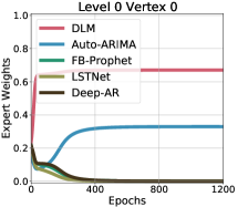
(a)

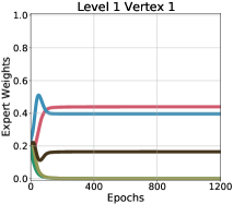
(b)

(c)

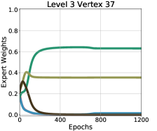
(d)

Figure 3: Pre-trained base models’ weight curve from vertices at different aggregation levels. The most suitable representation of each time series can be found in diverse combinations of base models.

Proposition 2 [Connection to Point Forecast] By setting the Chebyshev coefficient $C_{0}$ as

$$C_{0}=2\cdot\hat{x}_{t_{0}:T}-2\sum_{k=1,k~{}\mathrm{even}}^{d-1}(-1)^{k/2}~{}C_{k},$$ (4)

the point forecast $\hat{x}_{t_{0}:T}$ is the median of the distribution formed by the set of quantiles $\{q(\tau_{s})\}_{s=1}^{n}$.

Remark  Connecting to $\hat{x}_{t_{0}:T}$ calibrates quantile estimations to be consistent with point forecasts, which have been regularized to be near coherent across the hierarchy.

In summary, DYCHEM’s quantile estimation framework is to transform the direct estimation of $\{q(\tau_{s})\}_{s=1}^{n}$ into estimation of its components, Chebyshev coefficients, one of which ($C_{0}$) can be used to bind with point forecasts. We only require the input $x_{1:t_{0}}$ (for training function approximator $\phi$) and output $\hat{x}_{t_{0}:T}$ (for computing coefficient $C_{0}$) of the point prediction module and are therefore not dependent on which point prediction model we choose. Compared with directly estimating $\{q(\tau_{s})\}_{s=1}^{n}$, this procedure improves quantile estimations at each level by 1. eliminating quantile crossing; 2. improving quantile coherency: they are both difficult in regular quantile regression. Figure 2 wraps up the overall structure of DYCHEM.

IV Experiments

In this section, we provide a comprehensive evaluation of DYCHEM. Our experiments include: 1. coherent forecasts on hierarchically aggregated time series data (section IV-A - IV-C); 2. real-time forecasting under change of time series dynamics (section IV-D); 3. forecasting massive financial records on an industry forecasting pipeline IV-E. Our results show that DYCHEM can significantly improve forecasting performance over baselines and is adaptive to change of dynamics. Implementations of DYCHEM along its baselines, datasets and hyper-parameters of all following experiments can be found at github.com/aaronhan223/htsf.

Data $\backslash$ Method	Level	DYCHEM-LOO	SHARQ	HIER-E2E	Average	DYCHEM
Labour	1	43.33 $\pm$0.42 (.054)	52.07 $\pm$0.45 (.085)	45.12 $\pm$0.23 (.085)	49.34 $\pm$0.65 (.075)	38.84 $\pm$0.04 (.045)
	2	53.68 $\pm$0.68 (.104)	58.69 $\pm$0.41 (.120)	55.61 $\pm$0.74 (.107)	60.87 $\pm$0.33 (.119)	48.64 $\pm$0.78 (.092)
	3	57.16 $\pm$0.25 (.135)	64.02 $\pm$0.09 (.132)	60.03 $\pm$0.26 (.134)	69.29 $\pm$0.42 (.138)	49.17 $\pm$0.36 (.144)
	4	65.05 $\pm$0.18 (.153)	72.13 $\pm$0.34 (.167)	71.38 $\pm$0.15 (.154)	75.56 $\pm$0.94 (.156)	61.22 $\pm$0.14 (.163)
M5	1	49.29 $\pm$0.34 (.071)	56.31 $\pm$0.17 (.054)	51.69 $\pm$0.05 (.070)	59.61 $\pm$0.38 (.104)	42.61 $\pm$0.14 (.046)
	2	54.36 $\pm$0.28 (.127)	62.16 $\pm$0.27 (.079)	54.72 $\pm$0.63 (.116)	60.48 $\pm$0.58 (.133)	49.75 $\pm$0.22 (.084)
	3	55.18 $\pm$0.22 (.142)	65.37 $\pm$0.63 (.134)	65.02 $\pm$0.24 (.142)	68.29 $\pm$0.25 (.143)	53.61 $\pm$0.42 (.101)
	4	59.04 $\pm$0.36 (.164)	72.86 $\pm$0.27 (.189)	72.04 $\pm$0.36 (.164)	70.29 $\pm$0.34 (.168)	57.89 $\pm$0.47 (.109)
AEDemand	1	61.35 $\pm$0.76 (.132)	68.19 $\pm$0.29 (.113)	64.45 $\pm$0.48 (.213)	67.32 $\pm$0.29 (.164)	59.89 $\pm$0.32 (.145)
	2	58.12 $\pm$0.46 (.152)	66.57 $\pm$0.24 (.199)	63.72 $\pm$0.36(.131)	63.58 $\pm$0.72 (.129)	55.72 $\pm$0.73 (.122)
	3	66.38 $\pm$0.78 (.124)	68.25 $\pm$0.47 (.131)	68.01 $\pm$0.22 (.126)	70.44 $\pm$0.09 (.124)	62.55 $\pm$0.14 (.111)
	4	76.58 $\pm$0.63 (.136)	87.35 $\pm$0.69 (.225)	82.47 $\pm$0.28 (.192)	73.22 $\pm$0.37 (.135)	71.45 $\pm$0.43 (.125)
Wiki	1	65.98 $\pm$0.22 (.121)	70.36 $\pm$0.24 (.147)	69.67 $\pm$0.58 (.067)	66.42 $\pm$0.16 (.128)	63.27 $\pm$0.73 (.117)
	2	68.54 $\pm$0.47 (.157)	73.06 $\pm$0.42 (.159)	68.24 $\pm$0.33 (.108)	72.01 $\pm$0.52 (.157)	65.14 $\pm$0.46 (.143)
	3	72.42 $\pm$0.36 (.149)	76.15 $\pm$0.34 (.135)	74.62 $\pm$0.19 (.155)	74.37 $\pm$0.83 (.147)	69.48 $\pm$0.33 (.156)
	4	77.12 $\pm$0.23 (.268)	78.42 $\pm$0.34 (.201)	79.63 $\pm$0.41 (.291)	81.38 $\pm$0.65 (.278)	75.69 $\pm$0.76 (.189)
	5	84.77 $\pm$0.49 (.241)	85.12 $\pm$0.62 (.345)	79.65 $\pm$0.24 (.326)	84.68 $\pm$0.42 (.221)	76.88 $\pm$0.72 (.213)

TABLE I: Forecasting performance measured by averaged $\mathrm{MASE}^{\downarrow}$ and $\mathrm{CRPS}^{\downarrow}$ (within bracket) on 4 HTS datasets. M5 has more than 4 levels, we report results on the top 4 levels due to space constraint. All experiments are repeated 5 times.

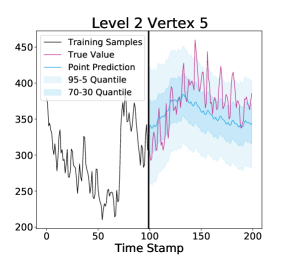
(a)

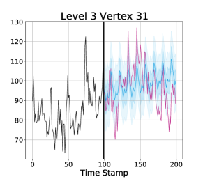
(b)

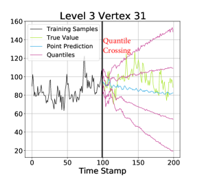
(c)

Figure 4: (a), (b) Quantile forecasting results generated by DYCHEM at vertex 5 and 31 of the Australian Labour data, where $\tau_{s}=[0.05,0.3,0.5,0.7,0.95]$. (c) SHARQ at same $\tau_{s}$, results showing mild quantile crossing.

Evaluation Metrics  We employ a commonly used relative error measure called mean absolute scaled error (MASE) [14] to evaluate point forecast accuracy. We use continuous ranked probability score (CRPS) [23] to measure quantile estimations, where it has been shown that the CRPS and quantile loss are equivalent [29]. In addition, we define a coherency loss to measure the coherency of time series forecast on a given hierarchy with $m$ vertices

$$\mathrm{Coherency~{}Loss}=\frac{1}{h}\sum_{t=T}^{T+h}\sum_{i=1}^{m}|\hat{x}_{t}^{v_{i}}-\sum_{e_{i,k}\in E}\hat{x}_{t}^{v_{k}}|.$$ (5)

Choosing Diverse Base Models  Models for time series span a wide range of categories. ARIMA(p,d,q) [13] is able to model many time series with trend and seasonality components, but its performance is normally poor on long-term forecast and time series with change-points. Dynamic regression models [34] extend ARIMA by inclusion of other external variables, but the process requires expertise and experimentation. If all variables are concurrent, difficulties in forecasting external variables will result in poor forecasts. Deep Neural Networks [19, 26] can improve the ability to model complex data with enough history. However, it is difficult to obtain a single model that works well in all situations. We choose 5 commonly used forecasting models that span across the above-mentioned categories as the base model of DYCHEM, including dynamic linear models (DLM) [36], Auto-ARIMA [13], Facebook Prophet [34], LSTNet [19] and DeepAR [26]. Although there is no strict rule on how to choose base models, it is beneficial to diversify forecasting models as they can be complementary in most situations. Since LSTNet and DeepAR are global models [18], which learn across a set of time series, we only need to train one model for a certain hierarchy. The rest of the models are trained on univariate time series, where we assign one model for each vertex. In the following experiments, we will show that the cooperation of these models will lead to significant improvement in forecasting.

IV-A Point Forecast

Experiment Setting  We compared with SHARQ [11] (LSTM as the base model), HIER-E2E [24], and ensemble averaging [4]. In addition, to show that a diverse set of base models brings more robustness to forecast, we perform leave-one-out (LOO) for every base model of DYCHEM and results are averaged across each run. We conducted our experiments on 4 public time-series datasets with hierarchical aggregations: Australian Labour, M5 [22], Wikipedia and AEDemand [2].

Figure 3 illustrates the weight evolution for each model as the gating network is trained and reconciled on vertices at each level using the Australian Labour dataset. According to the plots, the gating network emphasizes DLM for time series at the top aggregated level; as the level becomes lower, DLM becomes less dominant and other models begin to carry more weights at some vertices. Finally, at a bottom-level vertex where data becomes noisy, different models take charge of the forecast. The plots demonstrates individual contribution of each expert and the best way to represent different aggregated levels of HTS are distinct. Intuitively, learning weights from a richer space can improve the results over simple averaging. Table I shows level-wise point forecasting results measured by MASE. DYCHEM generates better results over baselines that includes single forecasting model (SHARQ and HIER-E2E), LOO for every base model, as well as combining models by ensemble averaging. The results shows that combining heterogeneous models through a gating network can significantly improve the forecasting accuracy. From Table I, we can also see that time series at lower aggregated levels are harder to forecast, given it is more likely to have sparsity issue.

IV-B Quantile Forecasts

We now evaluate the quantile forecasts after point forecasts are obtained. The neural network models $\phi$ are fed into mini-batches of training data $\mathrm{sw}(x_{1:t_{0}})$ generated by sliding windows, which are used to approximate Chebyshev coefficients. Each quantile estimation can then be computed recurrently and trained by quantile loss function. Figure 4 demonstrates quantile forecasting results on some arbitrary chosen vertices in Austrlian Labour dataset. Overall, the multi-quantile forecasts can well-capture the distribution of future time stamps at different aggregation levels, while the point forecasts binds the other quantiles by serving as the median of distribution. As a comparison, we also show an example of SHARQ trained with LSTM model, where the multiple quantile estimations are less constrained by the point forecast. Note that SHARQ is a very strong baseline, providing results superior to specific observation noise model such as Gaussian or negative binomial distribution. However, quantile crossing is possible since SHARQ cannot guarantee strict monotonicity w.r.t $\tau_{s}$. Table I quantitatively compares each method using CRPS: although the quantile forecasting results didn’t reach the same performance as point forecasts, DYCHEM still outperforms other baselines in the majority of situations.

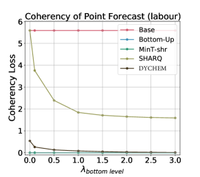
(a)

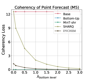
(b)

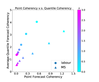
(c)

Figure 5: (a), (b) Absolute coherency loss of point forecast w.r.t. regularization strength $\lambda$ on Australian Labour and M5 dataset. (c) Relationship between point forecast coherency and average of quantile coherency.

IV-C Coherency Analysis

In our empirical studies, it is common that the absolute coherency loss defined by (5) cannot be completely eliminated, due to various reasons such as inappropriate choice of models or bad training of gating networks. We tune parameter $\lambda$ in Eq (1) that controls the penalty strength for coherency using bottom-level time series. For HTS with more than two aggregation levels, we progressively reduce $\lambda$ at higher levels based on the value of $\lambda_{\mathrm{bottom~{}level}}$, as higher level time series are easier to calibrate. We observe that by choosing $\lambda_{\mathrm{bottom~{}level}}$ in an appropriate range, coherency loss can be mitigated without sacrificing forecasting accuracy. We also compare with a few other baselines including Base method: regular time series forecast without reconciliation; Bottom-Up method: only forecast bottom-level time series and aggregate according to hierarchical structure to obtain higher level forecasts; MinT-shr: MinT with shrinkage estinator for covariance matrix. Figure 5 (a), (b) have shown that DYCHEM can achieve nearly coherent results. In fact, while DYCHEM significantly improves the accuracy of point forecast, it can also positively affect the coherency. Note that post-processing methods such as MinT, can reduce the coherency loss to a very small value at the cost of decreased accuracy, since the summation of bottom-level forecasts is “forced” to be aligned with higher-level forecasts. Figure 5 (c) shows that the improved coherency of point forecast can positively affect the coherency of quantiles. This result corresponds to our claim on Proposition 2. However, since the additive property does not hold for quantiles [11], there still exists non-zero coherency loss in certain quantiles.

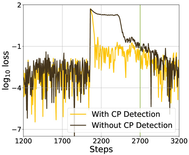
Figure 6: Online time series forecasting using DYCHEM under change-points.

IV-D Forecasting Under Change of Dynamics

In many applications, samples are collected sequentially, which requires the model to be updated in an online manner. It is possible that the change of dynamics will occur in such settings. We show that DYCHEM is robust when this is happened. Since gating network has been proven to be reasonably adaptive to abrupt changes [6], we further alleviate the jump of loss during the transient period in adapting to new dynamics with the help of Bayesian online change-point detection (BOCPD) [1]: after detecting change-points, we combine the original weights $\{w_{l}\}_{l=1}^{\mathsf{L}}$ with averaged weights $1/\mathsf{L}$ using a shrinkage factor that decreases exponentially through time. We assume new samples come with a batch size of 1; both gating network and models’ parameters are updated at each step. Fig. 6 shows the behaviour of DYCHEM when change-point occurs at around step 2050 and finally adapts to the new dynamics at step 2700. With the help of BOCPD, MSE loss during this transient period can be greatly reduced.

IV-E Forecasting Massive User Financial Records

DYCHEM has been tested within a large financial software company for cash flow forecasting. The hierarchy consists of 5 vertices, where the top level vertex represents the total expense of one user, the four bottom vertices are the first top, second top, third top and the rest of expenses of the corresponding user. We conducted experiments on 12,000 users’ data that possess the same hierarchy, and compared with already deployed baseline methods (PyDLM, PyDLM + MinT-shr) using normalised root mean squared error (NRMSE). DYCHEM significantly outperforms the deployed baselines. In addition, we have also modified DYCHEM for industrial deployment, which parallelized the training of forecasting models and gating networks at the same aggregated level given their mutual independence. Implementation and results can be found via the link provided in the beginning of section IV.

V Discussion

Forecasting hierarchically aggregated time series is an understudied problem with many applications. In this work, we propose DYCHEM that learns to combine a set of heterogeneous forecasting models while also performs quantile estimations in a model-free manner. DYCHEM has demonstrated superior results in both accuracy and coherency in HTS forecasting, and is adaptive to change of dynamics in sequential data. We also observed improvement of performance when deployed DYCHEM into an industry forecasting pipeline. In summary, DYCHEM produces forecasts that are more reliable, which are critical requirements for widespread adoption and safe deployment. The substantially more flexibility that DYCHEM offers in terms of using a customized mix of heterogeneous models for improving a specific time series forecast comes at an increased computational cost. It also introduces a few more hyper-parameters. Our future research will focus on ameliorating the costs when a large number of forecasts need to be done. In particular, we would like to further investigate situations where data resources are more constrained, such as short sequences or sequences with missing entries.

A. Proof of Proposition 1

• For each forecasting model, we obtain the following hierarchical forecasts which are not necessarily unbiased

  $$\hat{x}_{v_{1}}^{1}=\sum_{i=2}^{n}\hat{x}_{v_{i}}^{1}+\delta_{1};\quad\hat{x}_{v_{1}}^{2}=\sum_{i=2}^{n}\hat{x}_{v_{i}}^{2}+\delta_{2}~{}~{}\dots~{}~{}\hat{x}_{v_{1}}^{\mathsf{L}}=\sum_{i=2}^{n}\hat{x}_{v_{i}}^{\mathsf{L}}+\delta_{\mathsf{L}}.$$ (6)

  With out loss of generality, we assume $\hat{x}_{v_{i}}^{1}\leq\hat{x}_{v_{i}}^{2}\leq\dots\leq\hat{x}_{v_{i}}^{\mathsf{L}}$. The gating network generates a set of weights $\{w^{l}_{v_{i}}\}_{l=1}^{\mathsf{L}}\in[0,1]$ for models at vertex $v_{i}$ and $\{w_{l}\}_{l=1}^{\mathsf{L}}\in[0,1]$ on each coherency loss $\delta_{l}$ correspondingly. We can then rewrite Eq (6) as follows

  $$\sum_{l=1}^{\mathsf{L}}w_{v_{1}}^{l}\hat{x}_{v_{1}}^{l}=\sum_{i=2}^{n}\sum_{l=1}^{\mathsf{L}}w_{v_{i}}^{l}\hat{x}_{v_{i}}^{l}+\sum_{l=1}^{\mathsf{L}}w_{l}\delta_{l}.$$ (7)

  Since $\{\delta_{l}\}_{l=1}^{\mathsf{L}}$ cannot be all strictly positive or negative, we can therefore find a set of weights $\{w_{l}\}_{l=1}^{\mathsf{L}}\in[0,1]$ such that $\sum_{l=1}^{\mathsf{L}}w_{l}\delta_{l}=0,$ so DYCHEM is coherent.

Remark An equivalent statement of $\{\delta_{l}\}_{l=1}^{\mathsf{L}}$ do not have same sign is the forecasting ground truth value $x_{v_{i}}\in[\hat{x}_{v_{i}}^{1},\hat{x}_{v_{i}}^{\mathsf{L}}],\forall i\in[1,n]$. In other words, if $x_{v_{i}}$ can be written as the convex combination of each model’s forecast, DYCHEM can generate coherent forecasts. The convex hull assumption is much weaker than unbiased assumption used by other methods, making DYCHEM more robust to different applications.

B. Chebyshev Approximation

General Procedure

In order to train neural network $\phi$ using gradient-based methods, we first need to approximate the integral $\int_{-1}^{1}\phi(y)~{}dy$. We can transform this problem by a change of variable: $\int_{0}^{\pi}\phi(\cos\theta)\sin\theta~{}d\theta$. Define the Chebyshev polynomial $T_{k}:[-1,1]\rightarrow\mathbb{R}$ and its recurrent relationship

$$T_{0}(z)=1,~{}T_{1}(z)=z,~{}T_{k+1}(z)=2zT_{k}(z)-T_{k-1}(z),~{}k\geq 1,$$ (8)

which can also be written as $T_{k}(\cos\theta)=\cos(k\theta)$. By definition, we can write $\phi(\cos\theta)$ as its Chebyshev polynomial approximation [8]: $\phi(\cos\theta)=\frac{1}{2}c_{0}+\sum_{k=1}^{\infty}c_{k}\cdot T_{k}(\cos\theta)$, where $\{c_{k}\}_{k=0}^{\infty}$ are coefficients. Normally, a finite number of terms can achieve sufficient precision for approximation, e.g.

$$\phi(\cos\theta)\approx\frac{1}{2}~{}c_{0}+\sum_{k=1}^{d-1}~{}c_{k}\cdot T_{k}(\cos\theta)$$ (9)

is a $d$ degree Chebyshev polynomial approxiamtion of $\phi(\cos\theta)$. Therefore we have

$$\int_{0}^{\pi}\phi(\cos\theta)\sin\theta~{}d\theta =\int_{0}^{\pi}\phi(\cos\theta)~{}d\cos\theta$$

$$=\int_{-1}^{1}\left[\frac{1}{2}~{}c_{0}+\sum_{k=1}^{d-1}~{}c_{k}\cdot T_{k}(z)\right]~{}dz,$$

where $z=2\tau_{s}-1,\forall\tau_{s}\in[0,1]$. By the recurrent definition in Eq (8), the integral of the Chebyshev polynomial $T_{k}$ corresponds to a new Chebyshev polynomial: $\int T_{0}(z)~{}dz=T_{1}(z),~{}\int T_{1}(z)~{}dz=\frac{T_{2}(z)}{4}-\frac{T_{0}(z)}{4},~{}\int T_{k}(z)~{}dz=\frac{T_{k-1}(z)}{2(k-1)}-\frac{T_{k+1}(z)}{2(k+1)}.$ Therefore, the integration result can also be written in terms of Chebyshev polynomials: $\Phi(z)=\frac{1}{2}C_{0}+\sum_{k=1}^{d-1}C_{k}\cdot T_{k}(z)$, where the new coefficients $\{C_{k}\}_{k=1}^{d-1}$ can be obtained from the original coefficients by the following equations

$$C_{k}=\frac{c_{k-1}-c_{k+1}}{4k},~{}0<k<d-1,\quad C_{d-1}=\frac{c_{d-2}}{4(d-1)}.$$ (10)

The above derivation shows that the integral operation in Eq (2) can be replaced by Chebyshev polynomial approximation:

$$q(\tau_{s})=\sum_{k=1}^{d-1}C_{k}\cdot T_{k}(2\tau_{s}-1)+C_{0}.$$ (11)

Since the polynomials $T_{k}$ can be obtained in a recurrent manner instead of explicitly computed [8], estimating Chebyshev coefficients $\{c_{k}\}_{k=0}^{d-1}$ in Eq (9) is an important step.

Algorithm 1 Compute Chebyshev Coefficients

  Input: time series data $\mathrm{sw}(x_{1:t_{0}})$, Chebyshev polynomial degree $d$, MLP $\phi(\Theta_{q})$, point forecast $\hat{x}_{t_{0}:T}$, batch size $\mathrm{bs}$, window length $\omega$

  Process:

  $\{y_{k}\}_{k=0}^{d-1}=\cos\left(\frac{\pi(k+\frac{1}{2})}{d}\right),~{}~{}k\in[0,d)$  $\rhd$ Chebyshev roots

  $\mathcal{T}_{k}\leftarrow\texttt{Repeat}(\{y_{k}\}_{k=0}^{d-1},\lceil\frac{\mathrm{bs}}{d}\rceil+1)$  $\rhd$ repeat $y_{k}$ vector $\lceil\frac{\mathrm{bs}}{d}\rceil+1$ times

  $\mathrm{sw}(\mathcal{T}_{k})\in\mathbb{R}^{bs\times d}$  $\rhd$ generate $d$ vectors of roots by rolling window on $\mathcal{T}_{k}$ with step size 1

  for $j=0,\dots,d-1$ do

     $X_{j}\leftarrow\texttt{concat}[\mathrm{sw}(\mathcal{T}_{k})[:,j],~{}~{}\mathrm{sw}(x_{1:t_{0}})]\in\mathbb{R}^{\mathrm{bs}\times(\omega+1)}$  $\rhd$ combine different root values with time series and feed into model

     $O_{j}\leftarrow\phi_{j}(X_{j},\Theta_{q})$

     $P_{j}\leftarrow\texttt{softplus}(O_{j}+1e^{-5})+1e^{-3}$  $\rhd$ strictly positive outputs

  end for

  $\{c_{k}\}_{k=0}^{d-1}\leftarrow\texttt{DCT}(\{P_{j}\}_{j=0}^{d-1})$

  $\{C_{k}\}_{k=0}^{d-1}\leftarrow C_{k}=\frac{c_{k-1}-c_{k+1}}{4k},~{}~{}0<k<d-1,\quad C_{d-1}=\frac{c_{d-2}}{4(d-1)}$

  $C_{0}=2\cdot\hat{x}_{t_{0}:T}-2\sum_{k=1,k~{}\mathrm{even}}^{d-1}(-1)^{k/2}C_{k}$

  Return: $\{C_{k}\}_{k=0}^{d-1}$

Compute Chebyshev Coefficients

We evaluate $\phi(y,x_{1:t_{0}};\Theta_{q})$ at its $d$ uniformly distributed roots for $d$-dimension truncated Chebyshev polynomial approximation, i.e., $\{\phi(y_{k},x_{1:t_{0}};\Theta_{q})\}_{k=0}^{d-1}$. During implementation, we first use the sliding window approach to process the input data $x_{1:t_{0}}$, where $\mathrm{sw}(x_{1:t_{0}})$ can be processed by $\phi(\Theta_{q})$ in a common supervised learning way. $\{y_{k}\}_{k=0}^{d-1}$ serves as an additional feature of the input of $\phi(\Theta_{q})$, where $\phi(\Theta_{q}):\mathbb{R}^{\mathrm{bs}\times(\omega+1)}\rightarrow\mathbb{R}^{\mathrm{bs}\times 1}$ is implemented as a multilayer perceptron (MLP) with strictly positive output, where $\mathrm{bs}$ and $\omega$ represent the batch size and window length, respectively. Since the MLP should be evaluated at multiple roots, we combine $\mathrm{sw}(x_{1:t_{0}})\in\mathbb{R}^{\mathrm{bs}\times\omega}$ with different $\{t_{k}\}_{k=0}^{d-1}$ and feed them into $d$ replicates of MLP respectively. The outputs of $d$ MLP are then transformed by the Discrete Cosine Transform (DCT) algorithm to obtain the coefficients $\{c_{k}(x_{1:t_{0}})\}_{k=0}^{d-1}$. Full procedure in computing the Chebyshev coefficients can be found in Algorithm 1, which returns the set of coefficients $\{C_{k}\}_{k=0}^{d-1}$ with size $\mathbb{R}^{\mathrm{bs}\times d}$. These coefficients are then used to compute quantile values by iteratively combining with $T_{k}$ defined in Eq (8), where $z=2\tau_{s}-1\in[-1,1]$ and $\tau_{s}$ can be any specified quantiles.

C. Proof of Proposition 2

• If $\hat{x}_{t_{0}:T}$ is the median estimation, we have $q(0.5,x_{1:t_{0}})=\hat{x}_{t_{0}:T}$, since $T_{k}(0)=0$ when $k$ is odd and $T_{k}(0)=(-1)^{k/2}$ when $k$ is even, and

  $$q(0.5,x_{1:t_{0}})=\sum_{k=1}^{d-1}C_{k}(x_{1:t_{0}})\cdot T_{k}(0)+\frac{1}{2}C_{0}(x_{1:t_{0}},\hat{x}_{t_{0}:T}),$$ (12)

  we can therefore obtain the value of $C_{0}$ given the point forecasts are median:

  $$C_{0}(x_{1:t_{0}},\hat{x}_{t_{0}:T})=2\cdot\hat{x}_{t_{0}:T}-2\sum_{k=1,k~{}\mathrm{even}}^{d-1}(-1)^{k/2}C_{k}(x_{1:t_{0}}).$$ (13)

Remark Similarly, if $\hat{x}_{t_{0}:T}$ is determined to be the mean prediction, by definition we have

$$\int_{-1}^{1}z\cdot q(z)~{}dz =\int_{-1}^{1}z\cdot\left[\sum_{k=1}^{d-1}C_{k}\cdot T_{k}(z)+\frac{1}{2}C_{0}\right]dz$$

$$=\frac{1}{2}C_{0}+\sum_{k=1}^{d-1}C_{k}\int_{-1}^{1}z\cdot T_{k}(z)~{}dz.$$ (14)

Since Chebyshev polynomials are symmetric, we have

$$\int_{-1}^{1}z\cdot T_{k}(z)~{}dz=[1+(-1)^{k+1}]\int_{0}^{1}z\cdot T_{k}(z)~{}dz.$$ (15)

Then Eq (15) is zero if $k$ is even. Otherwise, according to the recurrence of Chebyshev polynomial

$$\int_{-1}^{1}z\cdot T_{k}(z)~{}dz=\left[\frac{T_{k-2}(z)}{2(k-2)}-\frac{T_{k+2}(z)}{2(k+2)}\right]\Bigg{|}_{0}^{1}=\frac{2}{k^{2}-4}.$$ (16)

Combine Eq (16) with Eq (14) and impose $\int_{-1}^{1}z\cdot q(z)~{}dz=\hat{x}_{t_{0}:T}$, we then have

$$C_{0}=2\cdot\hat{x}_{t_{0}:T}-4\sum_{k=1,k~{}\mathrm{odd}}^{d-1}\frac{C_{k}}{k^{2}-4}.$$ (17)

Appendix A Additional Results of IV-E

References

- [1] Ryan Prescott Adams and David JC MacKay. Bayesian online changepoint detection. arXiv preprint arXiv:0710.3742, 2007.
- [2] George Athanasopoulos, Rob J Hyndman, Nikolaos Kourentzes, and Fotios Petropoulos. Forecasting with temporal hierarchies. European Journal of Operational Research, 262(1):60–74, 2017.
- [3] Souhaib Ben Taieb and Bonsoo Koo. Regularized regression for hierarchical forecasting without unbiasedness conditions. In Proceedings of the 25th ACM SIGKDD International Conference on Knowledge Discovery & Data Mining, pages 1337–1347, 2019.
- [4] Aadyot Bhatnagar, Paul Kassianik, Chenghao Liu, Tian Lan, Wenzhuo Yang, Rowan Cassius, Doyen Sahoo, Devansh Arpit, Sri Subramanian, Gerald Woo, et al. Merlion: A machine learning library for time series. arXiv preprint arXiv:2109.09265, 2021.
- [5] Charles Blundell, Julien Cornebise, Koray Kavukcuoglu, and Daan Wierstra. Weight uncertainty in neural network. In International Conference on Machine Learning, pages 1613–1622. PMLR, 2015.
- [6] Wassim S Chaer, Robert H Bishop, and Joydeep Ghosh. A mixture-of-experts framework for adaptive kalman filtering. IEEE Transactions on Systems, Man, and Cybernetics, Part B (Cybernetics), 27(3):452–464, 1997.
- [7] Ke Chen, Dahong Xie, and Huisheng Chi. Speaker identification based on the time-delay hierarchical mixture of experts. In Proceedings of ICNN’95-International Conference on Neural Networks, volume 4, pages 2062–2066. IEEE, 1995.
- [8] Charles W Clenshaw. A note on the summation of chebyshev series. Mathematics of Computation, 9(51):118–120, 1955.
- [9] Conor Durkan, Artur Bekasov, Iain Murray, and George Papamakarios. Neural spline flows. arXiv preprint arXiv:1906.04032, 2019.
- [10] Achintya Gopal and Aaron Key. Normalizing flows for calibration and recalibration, 2021.
- [11] Xing Han, Sambarta Dasgupta, and Joydeep Ghosh. Simultaneously reconciled quantile forecasting of hierarchically related time series. In International Conference on Artificial Intelligence and Statistics, pages 190–198. PMLR, 2021.
- [12] Rob J Hyndman, Roman A Ahmed, George Athanasopoulos, and Han Lin Shang. Optimal combination forecasts for hierarchical time series. Computational statistics & data analysis, 55(9):2579–2589, 2011.
- [13] Rob J Hyndman, Yeasmin Khandakar, et al. Automatic time series forecasting: the forecast package for r. Journal of statistical software, 27(3):1–22, 2008.
- [14] Rob J Hyndman and Anne B Koehler. Another look at measures of forecast accuracy. International journal of forecasting, 22(4):679–688, 2006.
- [15] Rob J Hyndman, Alan J Lee, and Earo Wang. Fast computation of reconciled forecasts for hierarchical and grouped time series. Computational statistics & data analysis, 97:16–32, 2016.
- [16] Tomoharu Iwata and Zoubin Ghahramani. Improving output uncertainty estimation and generalization in deep learning via neural network gaussian processes. arXiv preprint arXiv:1707.05922, 2017.
- [17] Robert A Jacobs, Michael I Jordan, Steven J Nowlan, and Geoffrey E Hinton. Adaptive mixtures of local experts. Neural computation, 3(1):79–87, 1991.
- [18] Tim Januschowski, Jan Gasthaus, Yuyang Wang, David Salinas, Valentin Flunkert, Michael Bohlke-Schneider, and Laurent Callot. Criteria for classifying forecasting methods. International Journal of Forecasting, 36(1):167–177, 2020.
- [19] Guokun Lai, Wei-Cheng Chang, Yiming Yang, and Hanxiao Liu. Modeling long-and short-term temporal patterns with deep neural networks. In The 41st International ACM SIGIR Conference on Research & Development in Information Retrieval, pages 95–104, 2018.
- [20] Benjamin E Lauderdale, Delia Bailey, Jack Blumenau, and Douglas Rivers. Model-based pre-election polling for national and sub-national outcomes in the us and uk. International Journal of Forecasting, 36(2):399–413, 2020.
- [21] Zhiwu Lu. A regularized minimum cross-entropy algorithm on mixtures of experts for time series prediction and curve detection. Pattern Recognition Letters, 27(9):947–955, 2006.
- [22] S Makridakis, E Spiliotis, and V Assimakopoulos. The m5 accuracy competition: Results, findings and conclusions. Int J Forecast, 2020.
- [23] James E Matheson and Robert L Winkler. Scoring rules for continuous probability distributions. Management science, 22(10):1087–1096, 1976.
- [24] Syama Sundar Rangapuram, Lucien D Werner, Konstantinos Benidis, Pedro Mercado, Jan Gasthaus, and Tim Januschowski. End-to-end learning of coherent probabilistic forecasts for hierarchical time series. In International Conference on Machine Learning, pages 8832–8843. PMLR, 2021.
- [25] Roopesh Ranjan and Tilmann Gneiting. Combining probability forecasts. Journal of the Royal Statistical Society: Series B (Statistical Methodology), 72(1):71–91, 2010.
- [26] David Salinas, Valentin Flunkert, Jan Gasthaus, and Tim Januschowski. Deepar: Probabilistic forecasting with autoregressive recurrent networks. International Journal of Forecasting, 36(3):1181–1191, 2020.
- [27] Matthias Seeger, David Salinas, and Valentin Flunkert. Bayesian intermittent demand forecasting for large inventories. In Proceedings of the 30th International Conference on Neural Information Processing Systems, pages 4653–4661, 2016.
- [28] Noam Shazeer, Azalia Mirhoseini, Krzysztof Maziarz, Andy Davis, Quoc Le, Geoffrey Hinton, and Jeff Dean. Outrageously large neural networks: The sparsely-gated mixture-of-experts layer. arXiv preprint arXiv:1701.06538, 2017.
- [29] Phillip Si, Allan Bishop, and Volodymyr Kuleshov. Autoregressive quantile flows for predictive uncertainty estimation. arXiv preprint arXiv:2112.04643, 2021.
- [30] Jeremy Smith and Kenneth F Wallis. A simple explanation of the forecast combination puzzle. Oxford Bulletin of Economics and Statistics, 71(3):331–355, 2009.
- [31] Shengyang Sun, Guodong Zhang, Jiaxin Shi, and Roger Grosse. Functional variational bayesian neural networks. arXiv preprint arXiv:1903.05779, 2019.
- [32] Natasa Tagasovska and David Lopez-Paz. Single-model uncertainties for deep learning. arXiv preprint arXiv:1811.00908, 2018.
- [33] Souhaib Ben Taieb, James W Taylor, and Rob J Hyndman. Coherent probabilistic forecasts for hierarchical time series. In International Conference on Machine Learning, pages 3348–3357. PMLR, 2017.
- [34] Sean J Taylor and Benjamin Letham. Forecasting at scale. The American Statistician, 72(1):37–45, 2018.
- [35] Andreas S Weigend, Morgan Mangeas, and Ashok N Srivastava. Nonlinear gated experts for time series: Discovering regimes and avoiding overfitting. International journal of neural systems, 6(04):373–399, 1995.
- [36] Mike West and Jeff Harrison. Bayesian forecasting and dynamic models. Springer Science & Business Media, 2006.
- [37] Shanika L Wickramasuriya, George Athanasopoulos, Rob J Hyndman, et al. Forecasting hierarchical and grouped time series through trace minimization. Department of Econometrics and Business Statistics, Monash University, 105, 2015.
- [38] Yan Yang and Jinwen Ma. A single loop em algorithm for the mixture of experts architecture. In International Symposium on Neural Networks, pages 959–968. Springer, 2009.
- [39] Liang Zhao, Feng Chen, Chang-Tien Lu, and Naren Ramakrishnan. Multi-resolution spatial event forecasting in social media. In 2016 IEEE 16th International Conference on Data Mining (ICDM), pages 689–698. IEEE, 2016.