How Should Pre-Trained Language Models Be Fine-Tuned Towards Adversarial Robustness?

Abstract

The fine-tuning of pre-trained language models has a great success in many NLP fields. Yet, it is strikingly vulnerable to adversarial examples, e.g., word substitution attacks using only synonyms can easily fool a BERT-based sentiment analysis model. In this paper, we demonstrate that adversarial training, the prevalent defense technique, does not directly fit a conventional fine-tuning scenario, because it suffers severely from catastrophic forgetting: failing to retain the generic and robust linguistic features that have already been captured by the pre-trained model. In this light, we propose Robust Informative Fine-Tuning (RIFT), a novel adversarial fine-tuning method from an information-theoretical perspective. In particular, RIFT encourages an objective model to retain the features learned from the pre-trained model throughout the entire fine-tuning process, whereas a conventional one only uses the pre-trained weights for initialization. Experimental results show that RIFT consistently outperforms the state-of-the-arts on two popular NLP tasks: sentiment analysis and natural language inference, under different attacks across various pre-trained language models. .

1 Introduction

Deep models are well-known to be vulnerable to adversarial examples [64, 19, 50, 35]. For instance, fine-tuned models pre-trained on very large corpora can be easily fooled by word substitution attacks using only synonyms [2, 58, 32, 12]. This has raised grand security challenges to modern NLP systems, such as spam filtering and malware detection, where pre-trained language models like BERT [11] are widely deployed.

Attack algorithms [19, 7, 76, 40, 2] aim to maliciously generate adversarial examples to fool a victim model, while adversarial defense aims at building robustness against them. Among the defense methods, adversarial training [64, 19, 48, 45] is the most effective one [3]. It updates model parameters using perturbed adversarial samples generated on-the-fly and yields consistently robust performance even against the challenging adaptive attacks [3, 68].

However, despite its effectiveness in training from scratch, adversarial training may not directly fit the current NLP paradigm, the fine-tuning of pre-trained language models. First, fine-tuning per se suffers from catastrophic forgetting [46, 18, 34], i.e., the resultant model tends to over-fit to a small fine-tuning data set, which may deviate too far from the pre-trained knowledge [25, 81]. Second, adversarially fine-tuned models are more likely to forget: adversarial samples are usually out-of-distribution [38, 63], thus they are generally inconsistent with the pre-trained model. As a result, adversarial fine-tuning fails to memorize all the robust and generic linguistic features already learned during pre-training [65, 57], which are however very beneficial for a robust objective model.

Addressing forgetting is essential for achieving a more robust objective model. Conventional wisdom such as pre-trained weight decay [8, 10] and random mixout [37] mitigates forgetting by constraining $l_{p}$ distance between the two models’ parameters. Though effective to some extent, however, it is limited because change in the model parameter space only serves as an imperfect proxy for that in the function space [5]. Besides, the extent to which an encoder fails to retain information also depends on the input distribution. Therefore, a better way to encourage memorization is favorable.

In this paper, we follow an information-theoretical lens to look into the forgetting problem: we employ mutual information to measure how well an objective model memorizes the useful features captured before. This motivates our novel adversarial fine-tuning method, Robust Informative Fine-Tuning (RIFT). In addition to fitting a down-stream task as conventions, RIFT maximizes the mutual information between the output of an objective model and that of the pre-trained model conditioned on the class label. It encourages an objective model to continuously retain useful information from the pre-trained one throughout the whole fine-tuning process, whereas the conventional one only makes use of the pre-trained weights for initialization. We illustrate the overall objective of RIFT in Figure 1 and summarize the major contributions of this paper as follows:

• To the best of our knowledge, we are the first to investigate the intensified phenomenon of catastrophic forgetting in the adversarial fine-tuning of pre-trained language models.

• To address the forgetting problem and achieve more robust models, we propose a novel approach named Robust Informative Fine-Tuning (RIFT) from an information-theoretical perspective. RIFT enables an objective model to retain robust and generic linguistic features throughout the whole fine-tuning process and thus enhance robustness against adversarial examples.

• We empirically evaluate RIFT on two prevailing NLP tasks, sentiment analysis and natural language inference, where RIFT consistently outperforms the state-of-the-arts in terms of robustness, under different attacks across various pre-trained language models.

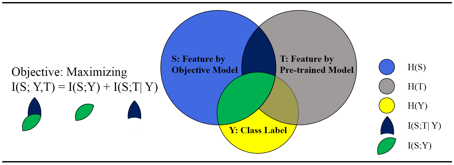
Figure 1: An illustration of the overall objective of RIFT. Maximizing $I(S;Y)$ encourages features of the objective model to be predictive of the class label, while maximizing $I(S;T|~{}Y)$ encourages learning robust and generic linguistic information from the pre-trained model. (Random variable $S$ denotes extracted features of $X$ by the objective model and $T$ by the pre-trained language model)

2 Methodology

2.1 Notations and Problem Setting

In this paper, we focus on the text classification task to introduce our method, while it can be easily extended to other NLP tasks. We suppose random variables $X,Y\sim p_{\mathcal{D}}(x,y)$, where $X$ represents the textual input, $Y$ represents the class label, $p_{\mathcal{D}}$ is the data distribution, and $x,y$ are the observed values. Our goal is to build a classifier $q(y|F_{s}(x))$, where $F_{s}(\cdot)$, referred to as our objective model in the rest of this paper, is a feature extractor fine-tuned from the encoder of a pre-trained language model, e.g., Transformer [72], and $q(\cdot|\cdot)$ is parameterized by using an MLP with softmaxed output. We favor a classifier that is robust against adversarial attacks [64, 2], i.e., maintaining high accuracy even given adversarial examples as inputs.

2.2 Adversarial Fine-Tuning Suffers From Forgetting

Adversarial training [64, 19, 45] is currently the most effective defense technique [3]. Its training objective can be generally formulated as:

$$\min[\mathop{\mathbb{E}}\limits_{x,y\sim p_{\mathcal{D}}}[\max\limits_{~{}\hat{x}\in\mathbb{B}(x)}\mathcal{L}(x,\hat{x},y)]],$$ (1)

where $\mathbb{B}(x)$ defines the allowed perturbation space around $x$, and $\mathcal{L}$ is a loss to encourage correct predictions both given vanilla samples and given perturbed examples. Such an objective function can also be applied to the fine-tuning of a pre-trained language model towards robustness, and we refer to it as adversarial fine-tuning. The loss function in Eq. 1 can be specified following Miyato et al. [48], Zhang et al. [79] in a semi-supervised fashion as:

$$-\log q(y|F_{s}(x))+\beta{\rm KL}\big{(}q(\cdot|F_{s}(x))||q(\cdot|F_{s}(\hat{x}))\big{)},$$ (2)

where the Kullback–Leibler divergence encourages invariant predictions between $x$ and $\hat{x}$.

(a) In adversarial fine-tuning, the relative $L_{2}$ dist-
ance continuously grows as the fine-tuning proceeds.

(b) Trading clean accuracy off against robustness (by increasing $\beta$ in Eq. 2) induces increased relative $L_{2}$ distance at the last epoch.

Figure 2: Relative $L_{2}$ distance between the pre-trained model and the objective model in the parameter space, under different fine-tuning schemes on IMDB, with small learning rate 2e-5.

Despite its effectiveness in training from scratch, such an adversarial objective function may not directly fit the fine-tuning scenario. To begin with, fine-tuning itself suffers from catastrophic forgetting [46, 18, 34]. During fine-tuning, an objective model $F_{s}(\cdot)$ tends to continuously deviate away from the pre-trained one to fit a down-stream task [25, 81], and thus the useful information already captured before is less utilized as the fine-tuning proceeds. Further, adversarial fine-tuning suffers even more from the forgetting problem, the reasons of which are given as what follows.

(i) Adversarial Fine-Tuning Tends to Forget: Adversarial fine-tuning targets at tackling adversarial examples, which are generally out of the manifold [38, 63] of the pre-training corpora. To additionally handle them, an objective model would be fine-tuned towards a solution that is far away from the optimization starting point, i.e., the pre-trained model. Figure 2 (b) empirically shows this point: by increasing $\beta$ in Eq. 2, we emphasize more on robustness instead of vanilla accuracy, and consequently, at the last epoch the distance between models also increases. Besides, adversarial fine-tuning often entails more iterations to converge (several times of normal fine-tuning), which further intensifies the forgetting problem, as the objective model is continuously deviating away as shown in Figure 2 (a).

(ii) Adversarial Fine-Tuning Needs to Memorize: Overfitting to training data is a dominant phenomenon throughout the adversarial training/fine-tuning process [60]. To mitigate overfitting and generalize better, adversarial fine-tuning should retain all the generalizable features already captured by the pre-trained model [11, 41]. In addition, adversarial fine-tuning favors an objective model that extracts features invariant to perturbations [70, 28] for robustness. As such, all those generalizable and robust linguistic information captured during pre-training [11, 65] are particularly beneficial and should be memorized. We empirically validates that encouraging memorization does improve both generalization and robustness in Sec. 3.5.

To address forgetting, previous methods such as pre-trained weight decay [8, 10] and random mixout [37] have shown their effectiveness in stabilizing fine-tuning [81]. However, they focus only on the parameter space, in which they encourage an object model to be similar to the pre-trained one. Distance in the parameter space can only approximately characterize the change in the function space, and fails to take the data distribution into consideration. A more natural way to capture the extent to which a model memorizes or forgets, should be using the mutual information between outputs of the two models, and we provide our solution as follows.

2.3 Informative Fine-Tuning

We first use an information-theoretical perspective to look into how a pre-trained model should be leveraged throughout the whole fine-tuning process.

We define random variable $T=F_{t}(X)$ as the feature of $X$ extracted by the pre-trained language model $F_{t}(\cdot)$, and $t$ as the observed value of $T$. Similarly, we define random variable $S=F_{s}(X)$ as the feature of $X$ extracted by our objective model $F_{s}(\cdot)$, and $s$ as the observed value of $S$. We formulate an overall fine-tuning objective as follows. The motivation is to train $F_{s}(\cdot)$ such that $S$ is capable of predicting $Y$, as well as preserving the information from $T$.

$$\max{I}(S;~{}Y,T),$$ (3)

i.e., maximizing the mutual information between (i) the feature extracted by the objective model and (ii) the class label plus the feature extracted by the pre-trained model. Since the pre-trained model $F_{t}(\cdot)$ is a fixed deterministic function, the fine-tuning objective in Eq. 3 in essense encourages $F_{s}(\cdot)$ to output features that contain as much information as possible for predicting $Y$ and $T$. This enables the objective model to learn from the pre-trained language model via $T$ throughout the whole fine-tuning process, and thus helps address the forgetting problem.

However, the objective defined in Eq. 3 is generally hard to optimize directly. Therefore, we decompose Eq. 3 into two terms as follows:

$${I}(S;~{}Y,T)={I}(S;Y)+{I}(S;T|~{}Y),$$ (4)

where ${I}(S;Y)$ measures how well the output of our objective model can predict the label, and ${I}(S;T|~{}Y)$ measures when conditioned on the class label, how well the output features of the two models can predict each other. Visualization of each component can be seen in Figure 1 for more intuitive understandings. We next introduce how each term in the right-hand side of Eq. 4 can be transformed into a tractable lower bound for optimization.

(i) Maximizing I(S;Y):  We treat $q(y|s)$, which is the classification layer that takes the features extracted by the objective model as input, as a variational distribution of $p(y|s)$, and derive a variational lower bound on ${I}(S;Y)$ following variational inference [33] as follows:

$${I}(S;Y) ={H}(Y)-{\mathbb{E}}_{x,y\sim p_{\mathcal{D}}}[-\log q(y|s)]+{\rm KL}\big{(}p(\cdot|s)||q(\cdot|s)\big{)}$$ (5)

$$\geq{H}(Y)-{\mathbb{E}}_{x,y\sim p_{\mathcal{D}}}[-\log q(y|s)],$$ (6)

where ${H}(Y)$ is a constant measuring the shannon entropy of $Y$, and ${\mathbb{E}}_{X,Y}[-\log q(y|s)]$ is essentially the cross-entropy loss using $q(y|s)$ for classification. Then, the objective of maximizing ${I}(S;Y)$ can be achieved by minimizing ${\mathbb{E}}_{X,Y}[-\log q(y|s)]$ instead.

(ii) Maximizing I(S;T| Y):  The definition of the conditional mutual information ${I}(S;T|~{}Y)$ is as follows:

$${I}(S;T|~{}Y)=\mathbb{E}_{y\sim p_{\mathcal{D}}(y)}[{I}(S;T)|~{}Y=y]=\mathbb{E}_{y\sim p_{\mathcal{D}}(y)}[~{}\mathbb{E}_{x\sim p_{\mathcal{D}}(x|y)}[\log\frac{p(s,t|y)}{p(s|y)p(t|y)}]].$$ (7)

To achieve a tractable objective for maximizing Eq. 7, we employ noise contrastive estimation [20, 49] and derive a lower bound $-\mathcal{L}_{\text{info}}$ on the conditional mutual information. This can be summarized in the following Lemma (the proof of which can be found in Appendix A.2):

Lemma 1.

Given $\{x_{i},y\}_{i=1}^{N}$ that is sampled i.i.d. from $p_{\mathcal{D}}(x|y)$, $s_{i}=F_{s}(x_{i})$, and $t_{i}=F_{t}(x_{i})$, ${I}(S;T|~{}Y)$ is lower bounded by $-\mathcal{L}_{\text{info}}=\mathbb{E}_{y\sim p_{\mathcal{D}}(y)}\big{[}\mathop{\mathbb{E}}_{\{x_{i},y\}_{i=1}^{N}}[\frac{1}{N}\sum_{i=1}^{N}\log\frac{e^{f_{y}(s_{i},t_{i})}}{\sum_{j=1}^{N}e^{f_{y}(s_{i},t_{j})}}+\log N]\big{]}$, and $f_{y}$ is a score function indexed by $y$.

By leveraging Lemma 1, $\mathcal{L}_{\text{info}}$ can be computed using a batch of samples and then minimized for maximizing ${I}(S;T|~{}Y)$. The score function $f_{y}$ is defined as the inner product after non-linear projections into a space of hyper-sphere following [9] as $f_{y}(a,b)=\frac{1}{\tau}\frac{\langle g_{y}^{1}(a),g_{y}^{2}(b)\rangle}{\|g_{y}^{1}(a)\|_{2}\|g_{y}^{2}(b)\|_{2}}$, where $g_{y}^{1}$ and $g_{y}^{2}$ are parameterized by using MLPs.

Figure 3: Visualization of the learned geometry using 500 random samples from IMDB by t-SNE [71]. $\blacktriangle$ and $\blacksquare$ denote samples from two different classes respectively. Different colors represent different data point IDs (approximately due to limited color space). In (c) and (d), $F_{s}(x)$ are projected to $\mathcal{S}^{1}$ with radius $1$, while $F_{t}(x)$ with radius $0.9$. For each sub-image: (a) The geometry of $F_{s}(x)$ before fine-tuning, represents the data manifold. (b) Maximizing $I(S;Y)$ encourages separating the whole data manifold into two class-specific data manifolds. (c) Maximizing $I(S;T)$ by contrastive loss in essence encourages alignment between two circles and uniformity over the whole data manifold. (d) Maximizing $I(S;T|~{}Y)$ by contrastive loss in essence encourages alignment and uniformity inside each class-specific data manifold. Best view in color with zooming in.

2.4 Conditional Mutual Information Better Fits A Down-Stream Task

Above we have introduced the training objective of informative fine-tuning and decomposed it into $I(S;Y)$ and $I(S;T|~{}Y)$ for optimization. However, one may wonder why not maximize $I(S;T)$ directly instead of $I(S;T|~{}Y)$. From an information-theoretical perspective, if we maximize $I(S;Y)$ and $I(S;T)$, the intersection of the three circles in Figure 1, i.e., the interaction information of them, is repeatedly optimized and might induce confliction. To further elaborate this point, we look into contrastive loss and give an explanation as follows.

We consider contrastive learning by decomposing it into the encouragement of alignment and uniformity following [74]. For example, maximizing $I(S;T)=H(S)-H(S|T)$ is to decrease $H(S|T)$ and increase $H(S)$. Decreasing $H(S|T)$ corresponds to encouraging alignment in contrastive learning, which aims to align $s_{i}$ and $t_{i}$ in the sense of inner product when they are projected into a hyper-sphere. In the meanwhile, increasing $H(S)$ corresponds to uniformity in contrastive learning, which encourages $s_{i}$ and $s_{j}$, where $i\neq j$, to diffuse over the whole sub-space as uniformly as possible. It can be seen in Figure 3 (c) that, in the space of $\mathcal{S}^{1}$, alignment is achieved in that points from two different circles but with the same color are aligned, and uniformity is achieved in that all points diffuse over the whole $\mathcal{S}^{1}$.

However, when maximizing $I(S;T)$, the uniformity in the contrastive loss is encouraged over the whole data manifold. Diffusing uniformly over the whole data manifold can be against the objective of maximizing $I(S;Y)$, which aims to separate the whole data manifold into class-specific parts as shown in Figure 3 (b). In contrast, maximizing $I(S;T|~{}Y)$ only encourages uniformity inside each class-specific data manifold, which is complementary to maximizing $I(S;Y)$, as show in Figure 3 (d). In the meanwhile, the alignment is still enforced. More empirical support can be found in Sec. 3.4.

2.5 Robust Informative Fine-Tuning

In this section, we are going to put the objective function of informative fine-tuning into the adversarial context and introduce Robust Informative Fine-Tuning (RIFT).

To robustly train a model, the adversarial examples $\hat{x}$ for training should be formulated and generated first. As our end goal is to enhance robustness in down-stream tasks, the generation process of adversarial examples should focus on preventing a model from predicting the ground truth label. However, using label for generating adversarial examples in training often induces label leaking [36], i.e., the generated adversarial examples contains label information which is used as a trivial short-cut by a classifier. As such, we follow [48, 79] to generate $\hat{x}$ in a self-supervised fashion:

$$\hat{x}=\underset{x^{\prime}\in\mathbb{B}(x)}{\arg\max}~{}{\rm KL}\big{(}q(\cdot|F_{s}(x))||q(\cdot|F_{s}(x^{\prime}))\big{)}.$$ (8)

By solving Eq. 8, $\hat{x}$ is found to induce the most different prediction from that of a vanilla sample $x$ in terms of KL, inside the attack space $\mathbb{B}(x)$.

Next, we introduce how to robustly optimize each objective in the informative fine-tuning by using $\hat{x}$.

Algorithm 1 RIFT

Input: dataset $\mathcal{D}$, hyper-parameters of AdamW [43]
Output: the model parameters $\theta$ and $\phi$

1:  Initialize $\theta$ using the pre-trained model, and initialize $\phi$ and $\varphi$ randomly.

2:  repeat

3:     Sample $y\sim p_{\mathcal{D}}(y)$ and then $\{x_{i},y\}_{i=1}^{N}\sim p_{\mathcal{D}}(x|y)$

4:     for  every $x_{i}$, $y$ in the mini-batch $\{x_{i},y\}_{i=1}^{N}$ do

5:        Find $\hat{x}_{i}$ by solving Eq. 8;

6:     end for

7:     Compute the loss function defined in Eq. 11 and update $\theta$, $\phi$, and $\varphi$ by gradients.

8:  until the training converges.

(i) Robustly Maximizing I(S;Y):  As shown in Sec. 2.3, maximizing ${I}(S;Y)$ can be achieved by minimizing a cross-entropy loss instead. To encourage adversarial robustness, this cross-entropy loss can be upgraded to encourage both correct predictions on and invariant predictions between $x$ and $\hat{x}$ [48, 79]. We formulate such an objective function as follows:

$$\min\limits_{\theta,\phi}\mathcal{L}_{\text{r-task}},~{}~{}~{}\mathcal{L}_{\text{r-task}}=\mathop{\mathbb{E}}\limits_{x,y\sim p_{\mathcal{D}}}\big{[}-\log q(y|F_{s}(x))+\beta{\rm KL}\big{(}q(\cdot|F_{s}(x))||q(\cdot|F_{s}(\hat{x}))\big{)}\big{]},$$ (9)

where $\theta$ denotes the parameters of $F_{s}(\cdot)$ and $\phi$ denotes the parameters of $q(\cdot|\cdot)$. Minimizing $\mathcal{L}_{\text{r-task}}$ in Eq. 9 corresponds to adversarilly maximizing $I(S;Y)$ for robust performance in a down-stream task. By doing so, the adversarial example $\hat{x}$ is generated by Eq. 8 first and then both $x$ and $\hat{x}$ are used to optimize the model parameters $\theta$ and $\phi$.

(ii) Robustly Maximizing I(S;T| Y):  We aim to maximize the conditional mutual information ${I}(S;T|~{}Y)$, but under an adversarial distribution of input data. We formulate such a term as ${I}(\hat{S};T|~{}Y)$, where random variable $\hat{S}=F_{s}(\hat{X})$, $\hat{X}\sim p_{\text{adv}}(\hat{x}|x,\theta,\phi,\mathbb{B})$, and sampling from $p_{\text{adv}}$, the adversarial distribution of input data, is to generate adversarial example $\hat{x}$ by Eq. 8.

To optimize ${I}(\hat{S};T|~{}Y)$, we propose $-\mathcal{L}_{\text{r-info}}$ as a lower bound on it, and formulate the objective to minimize $\mathcal{L}_{\text{r-info}}$ as follows (similar to $-\mathcal{L}_{\text{info}}$ by using Lemma 1):

$$\min\limits_{\theta,\varphi}\mathcal{L}_{\text{r-info}},~{}~{}~{}\mathcal{L}_{\text{r-info}}=\mathop{\mathbb{E}}\limits_{y\sim p_{\mathcal{D}}(y)}\big{[}\mathop{\mathbb{E}}\limits_{\{x_{i},y\}_{i=1}^{N}\sim p_{\mathcal{D}}(x|y)}[\frac{1}{N}\sum_{i=1}^{N}-\log\frac{e^{f_{y}(\hat{s}_{i},t_{i})}}{\sum_{j=1}^{N}e^{f_{y}(\hat{s}_{i},t_{j})}}-\log N]\big{]},$$ (10)

where $\hat{s}_{i}=F_{s}(\hat{x}_{i})$, $t_{i}=F_{t}(x_{i})$, and $\varphi$ denotes the parameters of all the score functions $f_{y}$. By Eq. 10, we are able to encourage $F_{s}(\cdot)$ to retain information from $F_{t}(\cdot)$ in a robust fasion.

Noted that, in $\mathcal{L}_{\text{r-info}}$ we do not use $\hat{x}_{i}$ to extract features from the pre-trained model. This follows the spirit of Knowledge Distillation [22] (though the setting is different in that a student is expected to perform identically to a teacher in knowledge distillation, while in fine-tuning it does not): the data used to extract features of a teacher should be inside the domain for which the teacher is trained. A down-stream NLP task, e.g., sentiment analysis, has a data domain that is generally a sub-domain of the pre-training corpora, while $\hat{x}_{i}$ can be significantly off the pre-training data manifold.

Objective Function of Robust Informative Fine-Tuning (RIFT):  The objective function of RIFT is a combination of $\mathcal{L}_{\text{r-task}}$ and $\mathcal{L}_{\text{r-info}}$, defined as follows:

$$\min\limits_{\theta,\phi,\varphi}\mathcal{L}_{\text{r-task}}+\alpha\mathcal{L}_{\text{r-info}},$$ (11)

where the hyper-parameter $\alpha$ controls to what extent we encourage an objective model to absorb information from the pre-trained one (ablation on $\alpha$ can be seen in Sec. 3.5). We summarize the whole training process in Algorithm 1 and include more implementation details in Appendix A.1.

3 Experiments

3.1 Experimental Setting

Tasks and Datasets: We evaluate the robust accuracy and compare our method with the state-of-the-arts on: (i) Sentiment analysis using the IMDB dataset [44]. (ii) Natural language inference using the SNLI dataset [6]. We mainly focus on robustness against adversarial word substitutions [2, 58], as such attacks preserve the syntactic and semantics very well [31, 78, 12], and are very hard to detect even by humans. Under this attack setting, any word in the input sequence can be substituted by a semantically similar word of it (often its synonym). We evaluate robustness on 1000 random examples from the testset of IMDB and SNLI respectively following [31, 12].

Model Architectures: We examine our methods and compare with state-of-the-arts on the following two prevailing pre-trained language models: (i) BERT-base-uncased [11]. (ii) RoBERTa-base [41].

Attack Algorithms: Two powerful attacks are employed: (i) Genetic [2] based on population algorithm. Aligned with [31, 12], the population size and iterations are set as $60$ and $40$ respectively. (ii) PWWS [58] based on word saliency. We only attack hypothesis on SNLI aligned with [31, 12].

Substitution Set: We follow [31, 12] to use the substitution set from [2], and the same language model constraint is applied to Genetic attacks and not to PWWS attacks.

Table 1: Accuracy(%) of different fine-tuning methods under attacks on IMDB.

Method	Model	Genetic	PWWS
Standard	BERT	38.1$\pm 2.5$	40.7$\pm 1.1$
Adv-Base	BERT	74.8$\pm 0.4$	68.3$\pm 0.3$
Adv-PTWD	BERT	73.9$\pm 0.4$	69.1$\pm 0.7$
Adv-Mixout	BERT	75.4$\pm 0.7$	68.8$\pm 0.6$
RIFT	BERT	77.2$\pm 0.8$	70.1$\pm 0.5$

(a) Accuracy (%) based on BERT-base-uncased.

Method	Model	Genetic	PWWS
Standard	RoBERTa	42.1$\pm 2.1$	45.6$\pm 3.1$
Adv-Base	RoBERTa	70.3$\pm 1.2$	63.3$\pm 0.7$
Adv-PTWD	RoBERTa	69.3$\pm 1.4$	64.4$\pm 0.3$
Adv-Mixout	RoBERTa	70.6$\pm 1.0$	63.9$\pm 1.3$
RIFT	RoBERTa	73.5$\pm 0.8$	66.3$\pm 0.7$

(b) Accuracy (%) based on RoBERTa-base.

Table 2: Accuracy(%) of different fine-tuning methods under attacks on SNLI.

Method	Model	Genetic	PWWS
Standard	BERT	40.1$\pm 0.7$	19.4$\pm 0.4$
Adv-Base	BERT	75.7$\pm 0.5$	72.9$\pm 0.2$
Adv-PTWD	BERT	75.2$\pm 1.0$	72.6$\pm 0.5$
Adv-Mixout	BERT	76.3$\pm 0.8$	73.2$\pm 1.0$
RIFT	BERT	77.5$\pm 0.9$	74.3$\pm 1.1$

(a) Accuracy (%) based on BERT-base-uncased.

Method	Model	Genetic	PWWS
Standard	RoBERTa	43.4$\pm 1.2$	20.4$\pm 1.0$
Adv-Base	RoBERTa	82.6$\pm 0.6$	79.9$\pm 0.7$
Adv-PTWD	RoBERTa	81.2$\pm 0.8$	78.9$\pm 0.7$
Adv-Mixout	RoBERTa	82.6$\pm 0.9$	80.6$\pm 0.3$
RIFT	RoBERTa	83.5$\pm 0.8$	81.1$\pm 0.4$

(b) Accuracy (%) based on RoBERTa-base.

3.2 Comparative Methods

(i) Standard Fine-Tuning: The standard fine-tuning process first initializes the objective model by the pre-trained weight, and then use cross-entropy loss to fine-tune the whole model.

(ii) Adversarial Fine-Tuning Baseline (Adv-Base): We employ the state-of-the-art defense against word substitutions, ASCC-Defense [12], as the adversarial fine-tuning baseline. This method is not initially proposed for pre-trained language models but can readily extend to perform adversarial fine-tuning. During fine-tuning, adversarial example $\hat{x}$, which is a sequence of convex combinations, is generated first and then both $x$ and $\hat{x}$ are used for optimization using objective defined in Eq. 9.

(iii) Adv + Pre-Trained Weight Decay (Adv-PTWD): Pre-trained weight decay [8, 10] penalizes $\lambda\|W_{\text{obj}}-W_{\text{pre}}\|_{2}$, and mitigates catastrophic forgetting [75, 37]. We combine it with the adversarial baseline for comparisons and $\lambda$ is chosen as $0.01$ on IMDB and $0.005$ on SNLI for best robustness.

(iv) Adv + Mixout (Adv-Mixout): Motivated by Dropout [62] and DropConnect [73], Mixout [37] is proposed to addresses catastrophic forgetting in fine-tuning. At each iteration each parameter is replaced by its pre-trained counter-part with probability $m$. We combine it with the adversarial fine-tuning baseline for comparisons with our method and $m$ is chosen as $0.6$ for best robustness.

(v) Robust Informative Fine-Tuning (RIFT): The proposed adversarial fine-tuning method. It can be deemed as the adversarial fine-tuning baseline plus the $\mathcal{L}_{\text{r-info}}$ term. We set $\tau$ as $0.2$ for all score functions $f_{y}$. For best robust accuracy, $\alpha$ is chosen as $0.1$ and $0.7$ on IMDB and SNLI respectively. Ablation study on $\alpha$ can be seen in Sec. 3.5.

For fair comparisons, all compared adversarial fine-tuning methods use the same $\beta$ on a same dataset, i.e., $\beta=10$ on IMDB and $\beta=5$ on SNLI, both of which are chosen for the best robust accuracy. Early stopping [60] is used for all compared methods according to best robust accuracy More implementation details and runtime analysis can be found in Appendix A.1 and A.3.

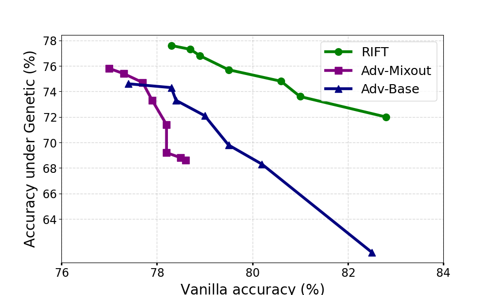
(a) Accuracy (%) under Genetic attacks.

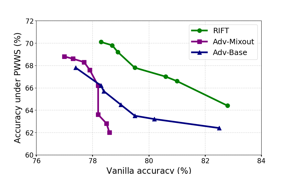
(b) Accuracy (%) under PWWS attacks.

Figure 4: Tradeoff curve between robustness and vanilla accuracy of BERT-based model on IMDB.

Table 3: Accuracy(%) of RIFT with maximizing $I(S;T|~{}Y)$ and $I(S;T)$ respectively.

Maximizing	Model	Genetic	PWWS
$\mathbf{I(S;T|~{}Y)}$	BERT	77.2	70.1
$I(S;T)$	BERT	76.1	69.4
$\mathbf{I(S;T|~{}Y)}$	RoBERTa	73.5	66.3
$I(S;T)$	RoBERTa	72.0	65.3

(a) Accuracy (%) under attacks on IMDB.

Maximizing	Model	Genetic	PWWS
$\mathbf{I(S;T|~{}Y)}$	BERT	77.5	74.3
$I(S;T)$	BERT	76.6	72.1
$\mathbf{I(S;T|~{}Y)}$	RoBERTa	83.5	81.1
$I(S;T)$	RoBERTa	82.5	79.4

(b) Accuracy (%) under attacks on SNLI.

3.3 Main Result

In this section we compare our method with state-of-the-arts by robustness under attacks. As shown in Tables 1 and 2(b)., RIFT consistently achieves the best robust performance among state-of-the-arts in all datasets across different pre-trained language models under all attacks. For instance, on IMDB our method outperforms the RoBERTa-based runner-up method by $2.9\%$ under Genetic attacks and $1.9\%$ under PWWS attacks. On SNLI based on BERT, we surpass the runner-up method by $1.2\%$ under Genetic attacks and $1.1\%$ under PWWS attacks. In addition, RIFT consistently improves robustness upon the adversarial fine-tuning baseline, while the improvements by other methods are not stable. We observe that on SNLI, we surpass the runner-up by a relatively small margin compared to IMDB. This may relate to the dataset property: input from SNLI has a smaller attack space (on average $6.5^{4}$ combinations of substitutions on SNLI compared to $6^{108}$ on IMDB), and thus smaller absolute space left for improvement. For results of vanilla accuracy please refer to Appendix A.4.

3.4 Conditional Mutual Information Does Fit a Down-Stream Task Better

In this section we empirically validate that maximizing $I(S;T|~{}Y)$ cooperates with a down-stream task better than maximizing $I(S;T)$ does. We plot two sets of results of our method with maximizing $I(S;T|~{}Y)$ and $I(S;T)$ respectively (using similar noise contrastive loss with all other hyper-parameters the same). As shown in Table 3(b), RIFT with maximizing $I(S;T|~{}Y)$ consistently outperforms that with maximizing $I(S;T)$ in terms of robustness under all attacks on both IMDB and SNLI, which serves as an empirical validation of Sec. 2.4.

Table 4: Ablation study on the hyper-parameter $\alpha$.

Parameter $\alpha$	Vanilla	Genetic	PWWS
0.00	78.1	74.8	68.3
0.05	78.4	76.5	69.2
0.10	78.3	77.2	70.1
0.30	78.3	76.2	69.5

(a) Acc (%) of RIFT based on BERT on IMDB.

Parameter $\alpha$	Vanilla	Genetic	PWWS
0.00	79.4	75.7	72.9
0.50	80.0	76.9	73.8
0.70	80.4	77.5	74.3
1.00	80.6	77.3	73.2

(b) Acc (%) of RIFT based on BERT on SNLI.

3.5 Ablation Study and Tradeoff Curve Between Robustness and Vanilla Accuracy

In this section we conduct ablation study on $\alpha$, which is the weight of $\mathcal{L}_{\text{r-info}}$ in Eq. 11. It aims to control to what extent the objective model absorbs information from the pre-trained one. As shown in Table 4, a good value of $\alpha$ improves both vanilla accuracy and robust accuracy; e.g., on IMDB increasing $\alpha$ from $0$ to $0.1$ results in increased vanilla accuracy by $0.2\%$ and increased robust accuracy under Genetic attacks by $2.4\%$. This demonstrates that RIFT does motivate the objective model to retain robust and generalizable features that are beneficial to both robustness and vanilla accuracy. When $\alpha$ goes too large, the objective of fine-tuning would focus too much on preserving as much information from the pre-trained model as possible, and thus ignores the down-stream task.

One may wonder whether informative fine-tuning itself can improve the clean accuracy upon normal fine-tuning. The answer is yes; e.g., on IMDB using RoBERTa, informative fine-tuning improves about $0.3\%$ clean accuracy upon normal fine-tuning baseline. The improvement is not very significant as normal fine-tuning targets at vanilla input only and thus suffers less from the forgetting problem. One common problem in contrastive loss is that the complexity grows quadratically with $N$, but larger $N$ contributes to tighter bound on the mutual information [49, 53]. One potential improvement is to maintain a dictionary updated on-the-fly like [21] and we will leave it for future exploration.

We finally show the trade-off curve between robustness and vanilla accuracy in Figure 4. As shown, RIFT outperforms the state-of-the-arts in terms of both robust accuracy and vanilla accuracy. It again validates that RIFT indeed helps the objective model capture robust and generalizable information to improve both robustness and vanilla accuracy, rather than trivially trading off one against another.

4 Related Work

Pre-Trained Language Models: Language modeling aims at estimating the probabilistic density of the textual data distribution. Classicial language modeling methods vary from CBOW, Skip-Gram [47], to GloVe [51] and ELMo [52]. Recently, Transformer [72] has demonstrated its power in language modeling, e.g., GPT [55] and BERT [11]. The representations learned by deep pre-trained language models are shown to be universal and highly generalizable [77] [41], and fine-tuning pre-trained language models becomes a paradigm in many NLP tasks [25, 11].

Adversarial Robustness: DNNs have achieved success in many fields, but they are susceptible to adversarial examples [64]. In NLP, attacks algorithms include char-level modifications [24, 13, 4, 17, 15, 54], sequence-level manipulations [29, 59, 30, 82], and adversarial word substitutions [2, 40, 58, 32, 80, 78]. For defenses, adversarial training [64, 19, 45] generates adversarial examples on-the-fly and is currently the most effective. Miyato et al. [48] first introduce adversarial training to NLP using $L_{2}$-ball to model perturbations, and later more geometry-aligned methods like first-order approximation[13], axis-aligned bound [31, 27], and convex hull [12], become favorable.

Fine-Tuning and Catastrophic Forgetting: The fine-tuning of pre-trained language models [25, 11] can be very unstable [11], as during fine-tuning the objective model can deviate too much from the pre-trained one, and easily over-fits to small fine-tuning sets [25]. Such phenomenon is referred as catastrophic forgetting [46, 18] in fine-tuning [25, 37, 81]. Methods to address catastrophic forgetting include pre-trained weight decay [8, 10, 81], learning rate decreasing [25], and Mixout regularization [37]. These methods focus on parameter space to constrain the distance between two models while our method addresses forgetting following an information-theoretical perspective. In continuous learning, method like rehearsal-based [42, 56, 39, 1] and regularization-based [34, 14, 26] also aims at the forgetting problem, but under a different setting: they focus on balanced performance on tasks with previous data, while in our setting the pre-training corpora are not available and language modeling is not our concern.

Contrastive Learning and Mutual Information: Contrastive learning [49, 23, 61] has demonstrated its power in learning self-supervised representations [9, 21]. The contrastive loss such as InfoNCE[49], InfoMax [23], is proposed as maximizing the mutual information of features in different views, and further discussed in [53, 67, 69, 66, 74]. This paper shares the same perspective of information theory, but looks into a different problem, addressing forgetting for fine-tuning. Addressing forgetting motivates our objective of maximizing the mutual information between the outputs of two models, which is different from conventional contrastive learning, and cooperation with fine-tuning motivates the use of conditional mutual information, which is quite different also. Fischer and Alemi [16] propose to restrict information for robustness in vision domain. Restricting information to some extent helps a model ignore spurious features, but may be at the cost of ignoring robust features as well. In contrast, the proposed method aims to retain the generic and robust features that are already captured by a pre-trained language model, and thus better fits a fine-tuning scenario.

5 Discussion and Conclusion

In this paper, we proposed RIFT to fine-tune a pre-trained language model towards robust down-stream performance. RIFT addresses the forgetting problem from an information-theoretical perspective and consistently outperforms state-of-the-arts in our experiments. We hope that this work can contribute to the NLP robustness in general and thus to more reliable NLP systems in real-life applications.

Appendix A Appendix

A.1 Implementation Details

Textual sequence processing. For consistent word numbers per input under word substitution attacks, we seperate word-level tokens by space and punctuations, and then follow the original tokenizer of BERT/RoBERTa to tokenize the input sequence. The byte-level RoBERTa tokenizer is further modified to output one token per word to fit the setting of word substitution attacks. The maximum number of tokens including special tokens per input is set as $300$ for IMDB, and $80$ for SNLI.

Hyper-parameters and optimization details. We set $\alpha$ as $0.1$ for IMDB and $0.7$ for SNLI. $\tau$ is set as $0.2$ for both IMDB and SNLI. Other hyper-parameters are set as the same among all compared methods for fair comparisons. For both standard fine-tuning and adversarial fine-tuning, we run for 20 epochs with batch size $32$ for IMDB, and run for 20 epochs with batch size $120$ for SNLI. Early stopping is used for all compared methods according to best robust accuracy. AdamW optimizer is employed with learning rate of $0.00002$. We do not apply weight decay on an objective model, and set weight decay rate as $0.0002$ for task-specific layers.

Model architectures. For both BERT and RoBERTa, the representation with respect to the sequence classification token of the last layer is employed as the output feature, which is later taken as the input of the task-specific layers for predictions. The task-specific layer is a MLP that has two linear layers with relu activation after the first layer and softmax after the second one.

Table 5: Vanilla Accuracy(%) of different fine-tuning methods on IMDB.

Method	Model	Vanilla Accuracy
Standard	BERT	93.1
Adv-Base	BERT	74.6
Adv-PTWD	BERT	76.6
Adv-Mixout	BERT	77.8
RIFT	BERT	78.3

(a) Accuracy (%) based on BERT-base-uncased.

Method	Model	Vanilla Accuracy
Standard	RoBERTa	94.9
Adv-Base	RoBERTa	80.1
Adv-PTWD	RoBERTa	80.7
Adv-Mixout	RoBERTa	79.0
RIFT	RoBERTa	84.2

(b) Accuracy (%) based on RoBERTa-base.

Table 6: Vanilla Accuracy(%) of different fine-tuning methods on SNLI.

Method	Model	Vanilla Accuracy
Standard	BERT	89.2
Adv-Base	BERT	79.4
Adv-PTWD	BERT	78.4
Adv-Mixout	BERT	79.3
RIFT	BERT	80.5

(a) Accuracy (%) based on BERT-base-uncased.

Method	Model	Vanilla Accuracy
Standard	RoBERTa	91.3
Adv-Base	RoBERTa	87.1
Adv-PTWD	RoBERTa	85.9
Adv-Mixout	RoBERTa	87.1
RIFT	RoBERTa	87.9

(b) Accuracy (%) based on RoBERTa-base.

A.2 The Proof of Lemma 1

The loss $\mathcal{L}_{\text{info}}$ is the categorical cross-entropy loss of identifying $t_{i}$ among $\{t_{j}\}_{j=1}^{N}$, given $s_{i}$ and $y$. Thus, the optimial $e^{f_{y}(s,t)}$ that minimizes $\mathcal{L}_{\text{info}}$ is proportional to $\frac{p(t|s,y)}{p(t|y)}$ (refer to [49] for more details). We then insert $\frac{p(t|s,y)}{p(t|y)}$ into $\mathcal{L}_{\text{info}}$ and get what follows:

$$\mathcal{L}_{\text{info}} =\mathop{\mathbb{E}}_{y\sim p_{\mathcal{D}}(y)}\big{[}\mathop{\mathbb{E}}_{\{x_{i},y\}_{i=1}^{N}}[\frac{1}{N}\sum_{i=1}^{N}-\log N\frac{\frac{p(t_{i}|s_{i},y)}{p(t_{i}|y)}}{\sum_{j=1}^{N}\frac{p(t_{j}|s_{i},y)}{p(t_{j}|y)}}]\big{]}$$ (12)

$$=\mathop{\mathbb{E}}_{y\sim p_{\mathcal{D}}(y)}\big{[}\mathop{\mathbb{E}}_{\{x_{i},y\}_{i=1}^{N}}[\frac{1}{N}\sum_{i=1}^{N}\log\frac{1}{N}\frac{\frac{p(t_{i}|s_{i},y)}{p(t_{i}|y)}+\sum_{j\neq i}^{N}\frac{p(t_{j}|s_{i},y)}{p(t_{j}|y)}}{\frac{p(t_{i}|s_{i},y)}{p(t_{i}|y)}}]\big{]}$$ (13)

$$=\mathop{\mathbb{E}}_{y\sim p_{\mathcal{D}}(y)}\big{[}\mathop{\mathbb{E}}_{\{x_{i},y\}_{i=1}^{N}}[\frac{1}{N}\sum_{i=1}^{N}\log\frac{1}{N}(1+{\frac{p(t_{i}|y)}{p(t_{i}|s_{i},y)}}{\sum_{j\neq i}^{N}\frac{p(t_{j}|s_{i},y)}{p(t_{j}|y)}})]\big{]}$$ (14)

$$=\mathop{\mathbb{E}}_{y\sim p_{\mathcal{D}}(y)}\big{[}\mathop{\mathbb{E}}_{\{x_{i},y\}_{i=1}^{N}}[\frac{1}{N}\sum_{i=1}^{N}\log(\frac{1}{N}+\frac{N-1}{N}{\mathop{\mathbb{E}}_{x\sim p_{\mathcal{D}}(x|y)}[\frac{p(t_{j}|s_{i},y)}{p(t_{j}|y)}]{\frac{p(t_{i}|y)}{p(t_{i}|s_{i},y)}}})]\big{]}$$ (15)

$$=\mathop{\mathbb{E}}_{y\sim p_{\mathcal{D}}(y)}\big{[}\mathop{\mathbb{E}}_{\{x_{i},y\}_{i=1}^{N}}[\frac{1}{N}\sum_{i=1}^{N}\log(\frac{1}{N}+\frac{N-1}{N}{\frac{p(t_{i}|y)}{p(t_{i}|s_{i},y)}})]\big{]}$$ (16)

$$\geq\mathop{\mathbb{E}}_{y\sim p_{\mathcal{D}}(y)}\big{[}\mathop{\mathbb{E}}_{\{x_{i},y\}_{i=1}^{N}}[\frac{1}{N}\sum_{i=1}^{N}\log{\frac{p(t_{i}|y)}{p(t_{i}|s_{i},y)}}]\big{]}$$ (17)

$$=\mathop{\mathbb{E}}_{y\sim p_{\mathcal{D}}(y)}\big{[}{\mathop{\mathbb{E}}_{x\sim p_{\mathcal{D}}(x|y)}}[-\log{\frac{p(t|s,y)}{p(t|y)}}]\big{]}$$ (18)

$$=-I(S;T|~{}Y).$$ (19)

Eq. 16 to Eq. 17 is by Jensen’s inequality. As such, $-\mathcal{L}_{\text{info}}$ is a lower bound on $I(S;T|~{}Y)$ and a larger $N$ makes the bound tighter. The specific design of the score function $f_{y}$ does not impact the correctness of Lemma 1: when $-\mathcal{L}_{\text{info}}$ is maximized, $-\mathcal{L}_{\text{info}}$ is still a lower bound on the mutual information term. However, if the capacity of $f_{y}$ is limited, the bound might be loose.

A.3 Runtime Analysis

All models are trained using the Nvidia A100 GPU and our implementation is based on PyTorch. As for IMDB, it takes about $10$ GPU hours to train a BERT or RoBERTa based model using RIFT. As for SNLI, it takes about $40$ GPU hours to train a BERT or RoBERTa based model using RIFT.

A.4 Vanilla Accuracy

we here show the vanilla accuracy of each methods in Tabs. 5 and 6(b) as a supplement. As we can see, RIFT surpasses all other adversarial fine-tuning method in terms of vanilla accuracy. It again validates that RIFT does help retain the generalizable information learned before.

A.5 License of Used Assets

The assets and the corresponding licenses are as follows. IMDB dataset [44]: Non-Commercial Licensing. SNLI dataset [6]: Creative Commons Attribution-ShareAlike 4.0 International License. Genetic attack [2]: MIT License. PWWS attack [58]: MIT License. Certified robustness [31]: MIT License. ASCC-defense [12]: MIT License.

References

- Aljundi et al. [2019] Rahaf Aljundi, Min Lin, Baptiste Goujaud, and Yoshua Bengio. Gradient based sample selection for online continual learning. In NeurIPS, 2019.
- Alzantot et al. [2018] Moustafa Alzantot, Yash Sharma, Ahmed Elgohary, Bo-Jhang Ho, Mani Srivastava, and Kai-Wei Chang. Generating natural language adversarial examples. In EMNLP, 2018.
- Athalye et al. [2018] Anish Athalye, Nicholas Carlini, and David Wagner. Obfuscated gradients give a false sense of security: Circumventing defenses to adversarial examples. In ICML, 2018.
- Belinkov and Bisk [2018] Yonatan Belinkov and Yonatan Bisk. Synthetic and natural noise both break neural machine translation. In ICLR, 2018.
- Benjamin et al. [2019] Ari S Benjamin, David Rolnick, and Konrad Kording. Measuring and regularizing networks in function space. In ICML, 2019.
- Bowman et al. [2015] Samuel R. Bowman, Gabor Angeli, Christopher Potts, and Christopher D. Manning. A large annotated corpus for learning natural language inference. In EMNLP, 2015.
- Carlini and Wagner [2017] Nicholas Carlini and David Wagner. Towards evaluating the robustness of neural networks. In SP, 2017.
- Chelba and Acero [2006] Ciprian Chelba and Alex Acero. Adaptation of maximum entropy capitalizer: Little data can help a lot. Computer Speech & Language, 20(4):382–399, 2006.
- Chen et al. [2020] Ting Chen, Simon Kornblith, Mohammad Norouzi, and Geoffrey Hinton. A simple framework for contrastive learning of visual representations. In ICML, 2020.
- Daumé III [2009] Hal Daumé III. Frustratingly easy domain adaptation. arXiv preprint arXiv:0907.1815, 2009.
- Devlin et al. [2019] Jacob Devlin, Ming-Wei Chang, Kenton Lee, and Kristina Toutanova. Bert: Pre-training of deep bidirectional transformers for language understanding. In NAACL, 2019.
- Dong et al. [2021] Xinshuai Dong, Anh Tuan Luu, Rongrong Ji, and Hong Liu. Towards robustness against natural language word substitutions. In ICLR, 2021.
- Ebrahimi et al. [2018] Javid Ebrahimi, Anyi Rao, Daniel Lowd, and Dejing Dou. Hotflip: White-box adversarial examples for text classification. In ACL, 2018.
- Ebrahimi et al. [2020] Sayna Ebrahimi, Mohamed Elhoseiny, Trevor Darrell, and Marcus Rohrbach. Uncertainty-guided continual learning with bayesian neural networks. In ICLR, 2020.
- Eger et al. [2019] Steffen Eger, Gözde Gül Şahin, Andreas Rücklé, Ji-Ung Lee, Claudia Schulz, Mohsen Mesgar, Krishnkant Swarnkar, Edwin Simpson, and Iryna Gurevych. Text processing like humans do: Visually attacking and shielding nlp systems. In NAACL, 2019.
- Fischer and Alemi [2020] Ian Fischer and Alexander A Alemi. Ceb improves model robustness. Entropy, 22(10):1081, 2020.
- Gao et al. [2018] Ji Gao, Jack Lanchantin, Mary Lou Soffa, and Yanjun Qi. Black-box generation of adversarial text sequences to evade deep learning classifiers. In SPW. IEEE, 2018.
- Goodfellow et al. [2013] Ian J Goodfellow, Mehdi Mirza, Da Xiao, Aaron Courville, and Yoshua Bengio. An empirical investigation of catastrophic forgetting in gradient-based neural networks. arXiv preprint arXiv:1312.6211, 2013.
- Goodfellow et al. [2015] Ian J Goodfellow, Jonathon Shlens, and Christian Szegedy. Explaining and harnessing adversarial examples. In ICLR, 2015.
- Gutmann and Hyvärinen [2010] Michael Gutmann and Aapo Hyvärinen. Noise-contrastive estimation: A new estimation principle for unnormalized statistical models. In AISTATS, 2010.
- He et al. [2020] Kaiming He, Haoqi Fan, Yuxin Wu, Saining Xie, and Ross Girshick. Momentum contrast for unsupervised visual representation learning. In Proceedings of the IEEE/CVF Conference on Computer Vision and Pattern Recognition, pages 9729–9738, 2020.
- Hinton et al. [2015] Geoffrey Hinton, Oriol Vinyals, and Jeff Dean. Distilling the knowledge in a neural network. arXiv preprint arXiv:1503.02531, 2015.
- Hjelm et al. [2019] R Devon Hjelm, Alex Fedorov, Samuel Lavoie-Marchildon, Karan Grewal, Phil Bachman, Adam Trischler, and Yoshua Bengio. Learning deep representations by mutual information estimation and maximization. In ICLR, 2019.
- Hosseini et al. [2017] Hossein Hosseini, Sreeram Kannan, Baosen Zhang, and Radha Poovendran. Deceiving google’s perspective api built for detecting toxic comments. arXiv preprint arXiv:1702.08138, 2017.
- Howard and Ruder [2018] Jeremy Howard and Sebastian Ruder. Universal language model fine-tuning for text classification. In ACL, 2018.
- Hu et al. [2021] Xinting Hu, Kaihua Tang, Chunyan Miao, Xian-Sheng Hua, and Hanwang Zhang. Distilling causal effect of data in class-incremental learning. In CVPR, 2021.
- Huang et al. [2019] Po-Sen Huang, Robert Stanforth, Johannes Welbl, Chris Dyer, Dani Yogatama, Sven Gowal, Krishnamurthy Dvijotham, and Pushmeet Kohli. Achieving verified robustness to symbol substitutions via interval bound propagation. In EMNLP, 2019.
- Ilyas et al. [2019] Andrew Ilyas, Shibani Santurkar, Dimitris Tsipras, Logan Engstrom, Brandon Tran, and Aleksander Madry. Adversarial examples are not bugs, they are features. arXiv preprint arXiv:1905.02175, 2019.
- Iyyer et al. [2018] Mohit Iyyer, John Wieting, Kevin Gimpel, and Luke Zettlemoyer. Adversarial example generation with syntactically controlled paraphrase networks. In NAACL, 2018.
- Jia and Liang [2017] Robin Jia and Percy Liang. Adversarial examples for evaluating reading comprehension systems. In EMNLP, 2017.
- Jia et al. [2019] Robin Jia, Aditi Raghunathan, Kerem Göksel, and Percy Liang. Certified robustness to adversarial word substitutions. In EMNLP, 2019.
- Jin et al. [2020] Di Jin, Zhijing Jin, Joey Tianyi Zhou, and Peter Szolovits. Is bert really robust? natural language attack on text classification and entailment. AAAI, 2020.
- Kingma and Welling [2013] Diederik P Kingma and Max Welling. Auto-encoding variational bayes. arXiv preprint arXiv:1312.6114, 2013.
- Kirkpatrick et al. [2017] James Kirkpatrick, Razvan Pascanu, Neil Rabinowitz, Joel Veness, Guillaume Desjardins, Andrei A Rusu, Kieran Milan, John Quan, Tiago Ramalho, Agnieszka Grabska-Barwinska, et al. Overcoming catastrophic forgetting in neural networks. Proceedings of the national academy of sciences, 114(13):3521–3526, 2017.
- Kurakin et al. [2016] Alexey Kurakin, Ian Goodfellow, and Samy Bengio. Adversarial examples in the physical world, 2016.
- Kurakin et al. [2017] Alexey Kurakin, Ian Goodfellow, and Samy Bengio. Adversarial machine learning at scale. In ICLR, 2017.
- Lee et al. [2020] Cheolhyoung Lee, Kyunghyun Cho, and Wanmo Kang. Mixout: Effective regularization to finetune large-scale pretrained language models. In ICLR, 2020.
- Li et al. [2019] Yingzhen Li, John Bradshaw, and Yash Sharma. Are generative classifiers more robust to adversarial attacks? In ICML, 2019.
- Li and Hoiem [2017] Zhizhong Li and Derek Hoiem. Learning without forgetting. IEEE transactions on pattern analysis and machine intelligence, 40(12):2935–2947, 2017.
- Liang et al. [2018] Bin Liang, Hongcheng Li, Miaoqiang Su, Pan Bian, Xirong Li, and Wenchang Shi. Deep text classification can be fooled. In IJCAI, 2018.
- Liu et al. [2019] Yinhan Liu, Myle Ott, Naman Goyal, Jingfei Du, Mandar Joshi, Danqi Chen, Omer Levy, Mike Lewis, Luke Zettlemoyer, and Veselin Stoyanov. Roberta: A robustly optimized bert pretraining approach. arXiv preprint arXiv:1907.11692, 2019.
- Lopez-Paz and Ranzato [2017] David Lopez-Paz and Marc’Aurelio Ranzato. Gradient episodic memory for continual learning. In NeurIPS, 2017.
- Loshchilov and Hutter [2019] Ilya Loshchilov and Frank Hutter. Decoupled weight decay regularization. In ICLR, 2019.
- Maas et al. [2011] Andrew L. Maas, Raymond E. Daly, Peter T. Pham, Dan Huang, Andrew Y. Ng, and Christopher Potts. Learning word vectors for sentiment analysis. In ACL, 2011.
- Madry et al. [2018] Aleksander Madry, Aleksandar Makelov, Ludwig Schmidt, Dimitris Tsipras, and Adrian Vladu. Towards deep learning models resistant to adversarial attacks. In ICLR, 2018.
- McCloskey and Cohen [1989] Michael McCloskey and Neal J Cohen. Catastrophic interference in connectionist networks: The sequential learning problem. In Psychology of learning and motivation. Elsevier, 1989.
- Mikolov et al. [2013] Tomas Mikolov, Ilya Sutskever, Kai Chen, Greg Corrado, and Jeffrey Dean. Distributed representations of words and phrases and their compositionality. In NeurIPS, 2013.
- Miyato et al. [2017] Takeru Miyato, Andrew M Dai, and Ian Goodfellow. Adversarial training methods for semi-supervised text classification. In ICLR, 2017.
- Oord et al. [2018] Aaron van den Oord, Yazhe Li, and Oriol Vinyals. Representation learning with contrastive predictive coding. arXiv preprint arXiv:1807.03748, 2018.
- Papernot et al. [2016] Nicolas Papernot, Patrick McDaniel, Somesh Jha, Matt Fredrikson, Z Berkay Celik, and Ananthram Swami. The limitations of deep learning in adversarial settings. In EuroS&P. IEEE, 2016.
- Pennington et al. [2014] Jeffrey Pennington, Richard Socher, and Christopher D Manning. Glove: Global vectors for word representation. In EMNLP, pages 1532–1543, 2014.
- Peters et al. [2018] Matthew E Peters, Mark Neumann, Mohit Iyyer, Matt Gardner, Christopher Clark, Kenton Lee, and Luke Zettlemoyer. Deep contextualized word representations. In NAACL-HLT, 2018.
- Poole et al. [2019] Ben Poole, Sherjil Ozair, Aaron Van Den Oord, Alex Alemi, and George Tucker. On variational bounds of mutual information. In ICML, 2019.
- Pruthi et al. [2019] Danish Pruthi, Bhuwan Dhingra, and Zachary C Lipton. Combating adversarial misspellings with robust word recognition. In ACL, 2019.
- Radford et al. [2018] Alec Radford, Karthik Narasimhan, Tim Salimans, and Ilya Sutskever. Improving language understanding by generative pre-training. https://s3-us-west-2.amazonaws.com/openai-assets/researchcovers/languageunsupervised/languageunderstandingpaper.pdf, 2018.
- Rebuffi et al. [2017] Sylvestre-Alvise Rebuffi, Alexander Kolesnikov, Georg Sperl, and Christoph H Lampert. icarl: Incremental classifier and representation learning. In CVPR, 2017.
- Reif et al. [2019] Emily Reif, Ann Yuan, Martin Wattenberg, Fernanda B Viegas, Andy Coenen, Adam Pearce, and Been Kim. Visualizing and measuring the geometry of bert. In NeurIPS, 2019.
- Ren et al. [2019] Shuhuai Ren, Yihe Deng, Kun He, and Wanxiang Che. Generating natural language adversarial examples through probability weighted word saliency. In ACL, 2019.
- Ribeiro et al. [2018] Marco Tulio Ribeiro, Sameer Singh, and Carlos Guestrin. Semantically equivalent adversarial rules for debugging nlp models. In ACL, 2018.
- Rice et al. [2020] Leslie Rice, Eric Wong, and Zico Kolter. Overfitting in adversarially robust deep learning. In ICML, 2020.
- Sohn [2016] Kihyuk Sohn. Improved deep metric learning with multi-class n-pair loss objective. In NeurIPS, 2016.
- Srivastava et al. [2014] Nitish Srivastava, Geoffrey Hinton, Alex Krizhevsky, Ilya Sutskever, and Ruslan Salakhutdinov. Dropout: a simple way to prevent neural networks from overfitting. The journal of machine learning research, 15(1):1929–1958, 2014.
- Stutz et al. [2019] David Stutz, Matthias Hein, and Bernt Schiele. Disentangling adversarial robustness and generalization. In CVPR, 2019.
- Szegedy et al. [2013] Christian Szegedy, Wojciech Zaremba, Ilya Sutskever, Joan Bruna, Dumitru Erhan, Ian Goodfellow, and Rob Fergus. Intriguing properties of neural networks. In ICLR, 2013.
- Tenney et al. [2019] Ian Tenney, Dipanjan Das, and Ellie Pavlick. Bert re-discovers the classical nlp pipeline. In ACL, 2019.
- Tian et al. [2020a] Yonglong Tian, Dilip Krishnan, and Phillip Isola. Contrastive representation distillation. In ICLR, 2020a.
- Tian et al. [2020b] Yonglong Tian, Chen Sun, Ben Poole, Dilip Krishnan, Cordelia Schmid, and Phillip Isola. What makes for good views for contrastive learning. In NeurIPS, 2020b.
- Tramer et al. [2020] Florian Tramer, Nicholas Carlini, Wieland Brendel, and Aleksander Madry. On adaptive attacks to adversarial example defenses. In NeurIPS, 2020.
- Tschannen et al. [2020] Michael Tschannen, Josip Djolonga, Paul K Rubenstein, Sylvain Gelly, and Mario Lucic. On mutual information maximization for representation learning. In ICLR, 2020.
- Tsipras et al. [2018] Dimitris Tsipras, Shibani Santurkar, Logan Engstrom, Alexander Turner, and Aleksander Madry. Robustness may be at odds with accuracy. arXiv preprint arXiv:1805.12152, 2018.
- Van der Maaten and Hinton [2008] Laurens Van der Maaten and Geoffrey Hinton. Visualizing data using t-sne. Journal of machine learning research, 9(11), 2008.
- Vaswani et al. [2017] Ashish Vaswani, Noam Shazeer, Niki Parmar, Jakob Uszkoreit, Llion Jones, Aidan N Gomez, Lukasz Kaiser, and Illia Polosukhin. Attention is all you need. In NeurIPS, 2017.
- Wan et al. [2013] Li Wan, Matthew Zeiler, Sixin Zhang, Yann Le Cun, and Rob Fergus. Regularization of neural networks using dropconnect. In ICML, 2013.
- Wang and Isola [2020] Tongzhou Wang and Phillip Isola. Understanding contrastive representation learning through alignment and uniformity on the hypersphere. In ICML, 2020.
- Wiese et al. [2017] Georg Wiese, Dirk Weissenborn, and Mariana Neves. Neural domain adaptation for biomedical question answering. In CoNLL, 2017.
- Wong et al. [2019] Eric Wong, Frank R Schmidt, and J Zico Kolter. Wasserstein adversarial examples via projected sinkhorn iterations. In ICML, 2019.
- Yang et al. [2019] Zhilin Yang, Zihang Dai, Yiming Yang, Jaime Carbonell, Ruslan Salakhutdinov, and Quoc V Le. Xlnet: Generalized autoregressive pretraining for language understanding. In NeurIPS, 2019.
- Zang et al. [2020] Yuan Zang, Fanchao Qi, Chenghao Yang, Zhiyuan Liu, Meng Zhang, Qun Liu, and Maosong Sun. Word-level textual adversarial attacking as combinatorial optimization. In ACL, 2020.
- Zhang et al. [2019a] Hongyang Zhang, Yaodong Yu, Jiantao Jiao, Eric P. Xing, Laurent El Ghaoui, and Michael I. Jordan. Theoretically principled trade-off between robustness and accuracy. In ICML, 2019a.
- Zhang et al. [2019b] Huangzhao Zhang, Hao Zhou, Ning Miao, and Lei Li. Generating fluent adversarial examples for natural languages. In ACL, 2019b.
- Zhang et al. [2021] Tianyi Zhang, Felix Wu, Arzoo Katiyar, Kilian Q Weinberger, and Yoav Artzi. Revisiting few-sample bert fine-tuning. In ICLR, 2021.
- Zhao et al. [2018] Zhengli Zhao, Dheeru Dua, and Sameer Singh. Generating natural adversarial examples. In ICLR, 2018.