Lyric document embeddings for music tagging

Abstract

We present an empirical study on embedding the lyrics of a song into a fixed-dimensional feature for the purpose of music tagging. Five methods of computing token-level and four methods of computing document-level representations are trained on an industrial-scale dataset of tens of millions of songs. We compare simple averaging of pretrained embeddings to modern recurrent and attention-based neural architectures. Evaluating on a wide range of tagging tasks such as genre classification, explicit content identification and era detection, we find that averaging word embeddings outperform more complex architectures in many downstream metrics.

1 Introduction

Song lyrics have been shown to be effective predictors of emotion [31], and can be indicative of genre [25, 3, 32, 15, 16, 14, 13], mood [7, 32, 6, 8, 11, 2], music exploration [29], song structure analysis [28] and other musical facets such as quality and release date [22, 19, 3]. This makes them good candidate features for automatic music tagging (assigning labels like pop, chill to songs).

In the literature Hu and Downie [7] use collections of $n$-gram word counts (along with audio) for classifying mood. Mayer et al. [14] classify genre via rhyme analysis of lyrics, and Van Zaanen and Kanters [26] re-weight the word counts using TF-IDF (see 2.2) to classify musical moods. Text in these studies is often represented in Bag of Words format [7, 14, 15], where a vocabulary is built from a corpus and a song is represented as counts of the corpus words [5]. To obtain a usable vocabulary size, words are typically removed from the corpus if they appeared too often (stopwords such as the, a) or not often enough (bespoke vocabulary and misspellings).

Bag of Words is a useful intuitive document representation, but does not account for the fact that some words may have a low count in a document, yet still be considered interesting from a corpus perspective (for example, the word algorithm in a corpus of agricultural documents). Term Frequency Inverse Document Frequency (TF-IDF) [9] accounts for this by multiplying Bag of Words by a factor representing how common a word is in a corpus, and has also been explored in the music tagging context [26].

The methods above have some clear drawbacks. First, no semantic meaning is preserved or inferred between the individual words, meaning for example the model shares no information between words such as love and adore. Second, the feature vectors can also easily become large and sparse (due to large vocabularies), making their use in machine learning models unwieldy. Word2vec [17] mitigates both of these issues by learning dense representations from a corpus, i.e. each word is represented as a point in a low-dimensional space in which semantically similar words are close. The training objective in this model is to predict either a missing word given the context (Continuous Bag of Words) or vice-versa (Skipgram). Word2vec has been adopted in a wide range of NLP tasks, including machine translation [24], sentiment analysis [33], and text generation [1]; and in the Music Information Retrieval (MIR) domain has successfully been applied to explicit song detection [20], genre classification [10] and music recommendation [27].

Although word order is considered in word2vec training, the algorithm does not provide a method for representing a document - something which is often needed for downstream tasks [3, 22]. One solution is to take summary statistics of the constituent word embeddings (i.e. simple averaging [27]). Another approach from the NLP literature is Doc2Vec [12], which learns paragraph-level representations of documents via an additional model input representing paragraph indices. Finally, it is possible to train the aggregation of word into document embeddings, for example using the final state of a recurrent neural network or the output of a self-attentive probe layer [30]. Advanced models such as these were used by Alexandros Tsaptsinos [25] to classify 20 music genres in a corpus of around 500,000 documents.

Solving these two problems (large vocabulary size and variable sequence lengths) is crucial to designing an accurate music tagging system from lyrics. Making this work practically, and at scale, is the subject of this paper. More concretely we investigate the efficaciousness off “off-the-shelf” language models trained on $\mathcal{O}(100B)$ tokens, training our own word embeddings from scratch on a bespoke lyrics dataset, and “warm-starting” the training. To produce a representation of an entire song, we evaluate whether word-level features should be averaged, or processed using recurrent architectures. It is out hope that this paper will serve as a practical guide for researchers hoping to make use of lyrics in tagging tasks.

2 Methods

The core of our investigation is trialling several options of representing song lyrics as an embedding. For this purpose we chose a transfer learning setup with distinct document embedding and tagging stages (Figure 1). This setup has benefits beyond our investigation: the document representation can be learned from massive amounts of unlabelled lyrics, and can be re-used for different downstream tasks. We describe the model components in detail below, beginning with some definitions.

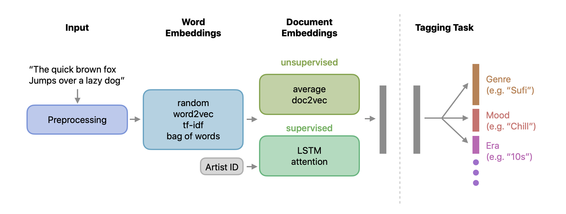
Figure 1: We begin by processing raw lyric strings, before generating embeddings at the word level. We then have various methods of computing document embeddings: both supervised (sequence models with artist identification as the target) and unsupervised (averaging and doc2vec). At the end of this process we have a single embedding per document, which is our proposed representation. We then evaluate these embeddings by training deep tagging classifiers on the same representation.

2.1 Definitions

In line with the NLP literature, we will refer to the lyrics to a song as a document, and to a collection of lyrics as a corpus. A document is made up of multiple words, usually broken by whitespace, but it is sometimes more convenient to work with subword tokens so that information can be shared between words like play, played, and playing in a model. Broader structural information within documents come in the form of sentences (groups of words separated by a period or other punctuation) or paragraphs (longer groups of words separated by line breaks). Lyrics do not often feature well-defined sentences but instead are arranged into lines and stanzas. As these are roughly analogous to sentences/paragraphs, so we will refer to them as such in the remainder of the paper.

2.2 Word embeddings

2.2.1 Baseline Models

We begin by defining some simple baseline models:

• random: random embeddings of dimension 128.

• bag-of-words-d: bag-of-words models with dimension $d$.

• tf-idf-d: TF-IDF models of dimension $d$.

For bag-of-words-d/tf-idf-d, we trimmed the vocabulary of the corpus by removing words which appeared in at least 90% of documents, and then retained the $d$ most commonly occurring words. We had initially planned to reduce the dimensionality of the baseline models in a more principled way through dimensionality reduction techniques such as Principal Component Analysis, but realized that even with a sparse implementation we could not scale these techniques to our dataset size.

2.2.2 Custom-trained word2vec

Next, we trained word2vec models on our dataset, using the Python package gensim to omit words which occurred fewer than five times in the dataset, and trained for 5 epochs – these hyperparameters seemed sensible enough that we did not attempt to optimize them. We did however try several embedding dimensions for use in downstream evaluation (see Table 2), and refer to these models as word2vec-d for dimensionality $d$.

2.2.3 Pre-trained word2vec

The appeal of pretrained embeddings is that they have been exposed to a massive amount of text – typically several orders of magnitude larger than in-house datasets. They can therefore learn a good general-purpose understanding of word semantics, which can then optionally be fine-tuned on a specific domain task. For our experiments we used the google news 300 dataset, which contains 300-dimensional vectors for around 3 million words, trained on around 100 Billion tokens [17]. Naturally some words appeared in our data for which no pretrained embedding existed - these were simply omitted. We refer to this model as google-300.

2.2.4 Warm-start word2vec

We also attempted to “warm-start” the training of the embeddings from the model above into new embeddings google-300-warm - these vectors retained their dimensionality and we kept the same training hyper-parameters as word2vec-d. The vocabularies of the two models were merged, such that words which appeared in both models took their initial state from google-300 whilst words which were unique to word2vec-d had random initial state.

2.3 Word Embedding Summaries

For all representations above, to obtain a document-level representation we used averaging (for word2vec-d) or the native summary statistic (e.g. summing word counts in a document for bag-of-words-d).

In order to take paragraph structure and/or word order into account when computing document embeddings, we make use of more sophisticated summarization techniques. This section investigates various methods for achieving this.

2.3.1 doc2vec

We begin with doc2vec [12], once again using the gensim implementation. We refer to these models as doc2vec-d.

2.3.2 LSTM and Attention

Next, we kept the best-performing word embeddings from Subsection 2.2 and experimented with two neural sequence models: Long Short Term Memory networks (lstm), and an attention network (attention). In order to learn the sequence parameters for these models, we needed a target for the model to predict. Not wanting to use any labels which would be later used in our evaluation framework (see 2.4), we decided to use the artist identifier as the target.

The number of unique artists in our dataset is naturally very large, so we considered using negative sampling [18] to simplify the task for the networks. However, we noticed in prior informal experiments that good results can actually be obtained with a large softmax layer instead. Practically speaking, we proceeded by selecting the $1,000$ most common artists in the dataset and computing their song counts. We then randomly sampled as many songs as we could for each of these artists such that we obtained a balanced dataset. The final state for lstm, or the aggregated embedding for attention, were then connected to the target with dense layers.

We defer the discussion of results until Section 4, but note here that both these models achieved a categorical accuracy in the artist identification proxy task of around 0.85. In the next Subsection we describe our tagging model and the datasets used to evaluate and compare different document embeddings.

2.4 Tagging Framework

2.4.1 Multi-label

Our tagging model is a multi-task neural network architecture, where predictions on different tag vocabularies are treated as different tasks. The input embedding is projected through a stack of fully connected layers until it branches to a number of linear output layers, one per tag vocabulary. The loss function used to train the network is obtained by summing the binary cross-entropy loss terms associated with the output branches. Note that binary cross-entropy loss is used instead of the categorical cross-entropy loss because multiple tags within the same vocabulary can be active for the same document.

2.4.2 Multi-task

We use multiple annotated datasets, defined over different set of documents: each dataset defines its own tag vocabulary and task. The multi-task formulation makes it convenient to handle missing annotations, while still training all tasks in parallel. The overall loss is:

$$\mathcal{L}_{d}=\sum_{i}\lambda_{i}a_{i,d}\mathcal{L}_{i,d},$$ (1)

where $\mathcal{L}_{i,d}$ is the loss term associated with the $i$-th task for document $d$, $\lambda_{i}$ the loss weight for the task, and $a_{i,d}\in[0,1]$ a binary flag that represents whether document $d$ is present in the annotations for task $i$. When a track does not appear in an annotation dataset, the loss terms associated with that dataset is set to zero.

2.4.3 Training

During training, mean Average Precision (mAP) is computed at each epoch, and training is stopped when mAP reaches a plateau on the validation set. Vocabulary-wise metrics are obtained simply by averaging the values for each tag, and a final scalar value is obtained by averaging across all tag vocabularies, weighted by the number of tags in each vocabulary. A summary of the hyper-parameters searched for all models is shown in Table 2.

3 Datasets

3.0.1 Lyrics datasets

We began with an internal dataset of 17,389,303 documents with primary language as English. Documents were then tokenized in gensim via the simple_preprocess function. We discovered that the distribution of number of tokens in the documents had an extremely long tail. This was prohibitive for sequence models, so for all document embedding experiments we truncated the number of tokens to 512, which reduced the maximum sequence length from 8,641 to 512 yet only affected 4% of documents. After preprocessing, we were left with a corpus of approximately 3.8 billion tokens.

3.0.2 Tagging datasets

We trained the tagging models on a set of internal datasets that were either manually curated or created from metadata. The datasets contain tags from different domains, e.g. genre, mood, release date, and are defined over different, but overlapping, set of documents. A description of the datasets is provided in Table 1.

					Examples per label
Dataset	Example tag	Tracks	Tags	Tags/track	Min	Mean	Max
Flagger	spoken	58,444	6	1	2,700	9,740	39,796
Era	10s	50,450	9	1	87	5,769	17,616
Moods	Chill	71,271	22	1.9	100	6,092	21,995
Explicit	True	48,683	2	1	16,234	24,241	32,449
Genre-1	Sufi	2,702,226	460	2.1	25	5,835	122,224
Genre-2	Piano	479,792	273	1	490	1,757	2,000
Genre-3	East Coast Rap	39,087	261	3.3	21	497	11,105
Genre-4	Worship	562,274	25	3.6	152	79,966	426,008

Table 1: Tag datasets used for evaluation. Tags/track is simply the number of tags per track, averaged over each dataset.

Some of the tag datasets may contain multiple labels for the same track, which makes creating balanced data splits more challenging. We used iterative splitting [21], while also forcing tracks from the same album to appear in the same split [4]. Note that some of the tagging datasets do overlap with the datasets used to train the document embeddings. However the risk of overfitting here is small because the only label we use for training our embeddings is the artist identifier (see Subsection 2.2).

4 Results

Hyperparameter	Values
embedding dimension	{$2^{7},\ldots,2^{9}$}
dropout	{$0.1,\ldots,0.9$}
learning rate	{$10^{-1},\ldots,10^{-5}$}
dense layers	{$2^{0},\ldots,2^{3}$}
dense size	{$2^{3},\ldots,2^{9}$}
lstm units	{$2^{6},\ldots,2^{9}$}
attention probes	{$2^{2},\ldots,2^{5}$}
attention mapping dimension	{$2^{2},\ldots,2^{5}$}

Table 2: Hyper-parameters evaluated in our experiments. Bayesian hyperparameter optimization [23] was used to optimize the validation mean Average Precision, with early stopping and patience of 10 epochs. 20 trials were run concurrently and in total 100 trials were conducted for each model.

4.1 Word embeddings

We show our results for overall mAP using word embeddings in Figure 2, showing only the best-performing model dimensionality in each group. All models outperform the random baseline but accuracy is varied across the tasks, owing in part to the differences in vocabulary size (recall Table 1). The word2vec-512 model with averaging achieves top performance on 6 of the 8 tasks, and is a close second on the Flagger task.

The only task on which a pretrained model is able to compete with word2vec-512 is on the Moods dataset. In general, warm-starting the training of embeddings did not yield improvements on our evaluation datasets.

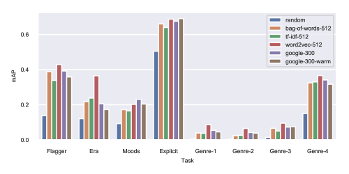
Figure 2: Word-level embedding experiments, showing mAP on each tagging task. Document embeddings obtained by averaging/summing embeddings across words.

4.2 Document embeddings

We selected word2vec-512 as our best-performing word-level embedder, and set out to see if we could improve over simple embedding averaging – see Table 3 for our results. Here we see that only attention is able to compete with word2vec-512, reaching similar performance on Genre-3 and superior scores on the Moods and Explicit datasets.

Given the ability of attention to effectively label moods and explicit content, it seems that artist identification was a suitable proxy task for training the sequence models, or that the attention architecture is well suited for tasks related with specific keywords, such as emotions for moods or offensive content for Explicit.

It is unclear why the powerful lstm/attention models do not yield higher scores. One reason could be that we have sufficient data to train excellent word embeddings, such that further refinements are simply hard to realize. With this in mind, and knowing that in many cases large amounts of data are difficult to come by, we were interested to see what kind of performance could be attained from subsets of our data.

	Flagger	Era	Moods	Explicit	Genre-1	Genre-2	Genre-3	Genre-4
word2vec-512	0.429	0.365	0.202	0.687	0.086	0.065	0.095	0.366
doc2vec-512	0.368	0.271	0.183	0.727	0.060	0.037	0.069	0.358
lstm	0.330	0.247	0.204	0.723	0.044	0.041	0.057	0.282
attention	0.427	0.295	0.272	0.760	0.070	0.057	0.107	0.350

Table 3: Mean average precision for each model and tagging dataset for computing document embeddings. Best results for each dataset are in boldface.

4.3 Incremental training

We trained word2vec-512 on random subsets of our data: 0.001%, 0.01%, 0.1%, 1%, 10%, retaining the full evaluation test set in each case. Results can be seen in Figure 3, and show that in fact over 80% of the mean average precision can be obtained from $1\%$ of the data (around 170,000 songs).

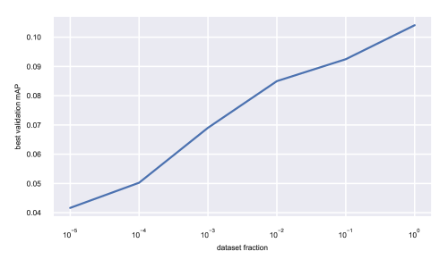
Figure 3: Effect of the dataset sample size on overall mean Average Precision for the tagging task and word2vec-512 model.

5 Conclusions

In this paper, we provided a comprehensive quantitative analysis of word2vec style embeddings for music tagging. On a range of challenging tagging tasks at the scale of millions of songs, we discovered that it is hard to surpass the performance of relatively simple models trained on in-house data. Small improvements to averaging embeddings were shown to be possible through sequence modelling, although results were not conclusive. Experiments on sampled data show that increasing training set size beyond $O$(1M) songs did not significantly improve tagging performance.

In future work, we are interested about the idea of extending our embedding framework to languages beyond English, and also seeing how useful our embeddings are as a source of side information in tasks such as music recommendation.

References

- [1] Tom B Brown, Benjamin Mann, Nick Ryder, Melanie Subbiah, Jared Kaplan, Prafulla Dhariwal, Arvind Neelakantan, Pranav Shyam, Girish Sastry, Amanda Askell, et al. Language models are few-shot learners. arXiv preprint arXiv:2005.14165, 2020.
- [2] Rémi Delbouys, Romain Hennequin, Francesco Piccoli, Jimena Royo-Letelier, and Manuel Moussallam. Music mood detection based on audio and lyrics with deep neural net. arXiv preprint arXiv:1809.07276, 2018.
- [3] Michael Fell and Caroline Sporleder. Lyrics-based analysis and classification of music. In Proceedings of COLING 2014, the 25th international conference on computational linguistics: Technical papers, pages 620–631, 2014.
- [4] Arthur Flexer and Dominik Schnitzer. Album and artist effects for audio similarity at the scale of the web. In Proceedings of the 6th Sound and Music Computing Conference (SMC-09, 2009.
- [5] Zellig S. Harris. Distributional structure. WORD, 10(2-3):146–162, 1954.
- [6] Xiao Hu and J Stephen Downie. Improving mood classification in music digital libraries by combining lyrics and audio. In Proceedings of the 10th annual joint conference on Digital libraries, pages 159–168, 2010.
- [7] Xiao Hu and J Stephen Downie. When lyrics outperform audio for music mood classification: A feature analysis. In ISMIR, pages 619–624, 2010.
- [8] Xiao Hu, J Stephen Downie, and Andreas F Ehmann. Lyric text mining in music mood classification. American music, 183(5,049):2–209, 2009.
- [9] Li-Ping Jing, Hou-Kuan Huang, and Hong-Bo Shi. Improved feature selection approach tfidf in text mining. In Proceedings. International Conference on Machine Learning and Cybernetics, volume 2, pages 944–946. IEEE, 2002.
- [10] Akshi Kumar, Arjun Rajpal, and Dushyant Rathore. Genre classification using word embeddings and deep learning. In 2018 International Conference on Advances in Computing, Communications and Informatics (ICACCI), pages 2142–2146. IEEE, 2018.
- [11] Cyril Laurier, Jens Grivolla, and Perfecto Herrera. Multimodal music mood classification using audio and lyrics. In 2008 Seventh International Conference on Machine Learning and Applications, pages 688–693. IEEE, 2008.
- [12] Quoc Le and Tomas Mikolov. Distributed representations of sentences and documents. In International conference on machine learning, pages 1188–1196. PMLR, 2014.
- [13] Rudolf Mayer, Robert Neumayer, and Andreas Rauber. Combination of audio and lyrics features for genre classification in digital audio collections. In Proceedings of the 16th ACM international conference on Multimedia, pages 159–168, 2008.
- [14] Rudolf Mayer, Robert Neumayer, and Andreas Rauber. Rhyme and style features for musical genre classification by song lyrics. In ISMIR, pages 337–342, 2008.
- [15] Rudolf Mayer and Andreas Rauber. Musical genre classification by ensembles of audio and lyrics features. In ISMIR, pages 675–680, 2011.
- [16] Cory McKay, John Ashley Burgoyne, Jason Hockman, Jordan BL Smith, Gabriel Vigliensoni, and Ichiro Fujinaga. Evaluating the genre classification performance of lyrical features relative to audio, symbolic and cultural features. In ISMIR, pages 213–218, 2010.
- [17] Tomas Mikolov, Kai Chen, Greg Corrado, and Jeffrey Dean. Efficient estimation of word representations in vector space. arXiv preprint arXiv:1301.3781, 2013.
- [18] Tomas Mikolov, Ilya Sutskever, Kai Chen, Greg Corrado, and Jeffrey Dean. Distributed representations of words and phrases and their compositionality. arXiv preprint arXiv:1310.4546, 2013.
- [19] Tom O’Hara, Nico Schüler, Yijuan Lu, and Dan Tamir. Inferring chord sequence meanings via lyrics: Process and evaluation. In ISMIR, pages 463–468, 2012.
- [20] Marco Rospocher. Explicit song lyrics detection with subword-enriched word embeddings. Expert Systems with Applications, 163:113749, 2021.
- [21] Konstantinos Sechidis, Grigorios Tsoumakas, and Ioannis Vlahavas. On the stratification of multi-label data. In Proceedings of the 2011 European Conference on Machine Learning and Knowledge Discovery in Databases, ECML PKDD’11, page 145–158, 2011.
- [22] Alex G Smith, Christopher XS Zee, and Alexandra L Uitdenbogerd. In your eyes: Identifying clichés in song lyrics. In Proceedings of the Australasian Language Technology Association Workshop 2012, pages 88–96, 2012.
- [23] Jasper Snoek, Hugo Larochelle, and Ryan P Adams. Practical bayesian optimization of machine learning algorithms. arXiv preprint arXiv:1206.2944, 2012.
- [24] Ilya Sutskever, Oriol Vinyals, and Quoc V Le. Sequence to sequence learning with neural networks. arXiv preprint arXiv:1409.3215, 2014.
- [25] Alexandros Tsaptsinos. Lyrics-based music genre classification using a hierarchical attention network. In ISMIR, 2017.
- [26] Menno Van Zaanen and Pieter Kanters. Automatic mood classification using tf* idf based on lyrics. In ISMIR, pages 75–80, 2010.
- [27] Michaela Vystrčilová and Ladislav Peška. Lyrics or audio for music recommendation? In Proceedings of the 10th International Conference on Web Intelligence, Mining and Semantics, pages 190–194, 2020.
- [28] Kento Watanabe and Masataka Goto. A chorus-section detection method for lyrics text. pages 351–359.
- [29] Kento Watanabe and Masataka Goto. Query-by-blending: A music exploration system blending latent vector representations of lyric word, song audio, and artist. In ISMIR, pages 144–151, 2019.
- [30] Guangxu Xun, Kishlay Jha, Ye Yuan, Yaqing Wang, and Aidong Zhang. Meshprobenet: a self-attentive probe net for mesh indexing. Bioinformatics, 35(19):3794–3802, 2019.
- [31] Dan Yang and Won-Sook Lee. Music emotion identification from lyrics. In 2009 11th IEEE International Symposium on Multimedia, pages 624–629. IEEE, 2009.
- [32] Teh Chao Ying, Shyamala Doraisamy, and Lili Nurliyana Abdullah. Genre and mood classification using lyric features. In 2012 International Conference on Information Retrieval & Knowledge Management, pages 260–263. IEEE, 2012.
- [33] Lei Zhang, Shuai Wang, and Bing Liu. Deep learning for sentiment analysis: A survey. Wiley Interdisciplinary Reviews: Data Mining and Knowledge Discovery, 8(4):e1253, 2018.