Learned Queries for Efficient Local Attention

Abstract

Vision Transformers (ViT) serve as powerful vision models. Unlike convolutional neural networks, which dominated vision research in previous years, vision transformers enjoy the ability to capture long-range dependencies in the data. Nonetheless, an integral part of any transformer architecture, the self-attention mechanism, suffers from high latency and inefficient memory utilization, making it less suitable for high-resolution input images. To alleviate these shortcomings, hierarchical vision models locally employ self-attention on non-interleaving windows. This relaxation reduces the complexity to be linear in the input size; however, it limits the cross-window interaction, hurting the model performance. In this paper, we propose a new shift-invariant local attention layer, called query and attend (QnA), that aggregates the input locally in an overlapping manner, much like convolutions. The key idea behind QnA is to introduce learned queries, which allow fast and efficient implementation. We verify the effectiveness of our layer by incorporating it into a hierarchical vision transformer model. We show improvements in speed and memory complexity while achieving comparable accuracy with state-of-the-art models. Finally, our layer scales especially well with window size, requiring up-to x10 less memory while being up-to x5 faster than existing methods. The code is publicly available at https://github.com/moabarar/qna.

1 Introduction

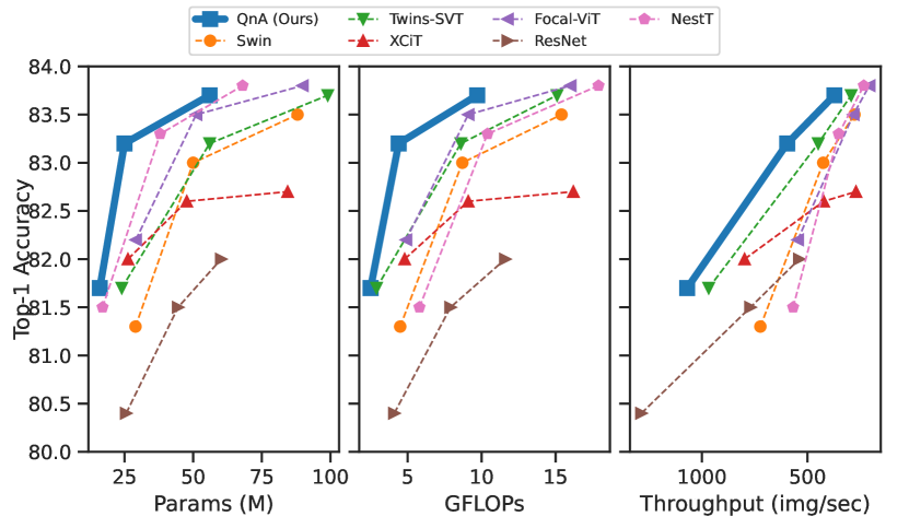
Figure 1: Performance-Efficiency Comparisons On $224^{2}$ Input Size. QnA-ViT (our method) demonstrates better accuracy-efficiency trade-off compared to state-of-the-art baselines. As suggested by Dehghani et al. [15], we report the ImageNet-1k [58] Top-1 accuracy (y-axis) trade-off with respect to parameter count (left), floating point operations (middle) and inference throughput (right). The throughput is measured using the timm [73] library, as tested on NVIDIA V100 with 16GB memory. Other metrics, are from the original publications [45, 11, 82, 89, 74, 19]

Two key players take the stage when considering data aggregation mechanisms for image processing. Convolutions were the immediate option of choice. They provide locality, which is an established prior for image processing, and efficiency while doing so. Nevertheless, convolutions capture local patterns, and extending them to global context is difficult if not impractical. Attention-based models [70], on the other hand, offer an adaptive aggregation mechanism, where the aggregation scheme itself is input-dependent, or spatially dynamic. These models [17, 6] are the de-facto choice in the natural-language processing field and have recently blossomed for vision tasks as well.

Earlier variants of the Vision Transformers (ViT) [18] provide global context by processing non-interleaving image patches as word tokens. For these models to be effective, they usually require a vast amount of data [18, 61], heavy regularization [65, 60] or modified optimization objectives [10, 21]. Even more so, it was observed that large scale-training drives the models to attend locally [56], especially for early layers, encouraging the notion that locality is a strong prior.

Local attention mechanisms are the current method of choice for better vision backbones. These backbones follow a pyramid structure similar to convolutional neural networks (CNNs) [72, 11, 20, 89], and process high-resolution inputs by restricting the self-attention to smaller windows, preferably with some overlap [69] or other forms of inter-communication [45, 82, 11]. The latter approaches naturally induce locality while benefiting from spatially dynamic aggregation. On the other hand, these architectures come at the cost of computational overhead and, more importantly, are not shift-equivariant.

In this paper, we revisit the design of local attention and introduce a new aggregation layer called Query and Attend (QnA). The key idea is to leverage the locality and shift-invariance of convolutions and the expressive power of attention mechanisms.

In local self-attention, attention scores are computed between all elements comprising the window. This is a costly operation of quadratic complexity in the window size. We propose using learned queries to compute the aggregation weights, allowing linear memory complexity, regardless of the chosen window size. Our layer is also flexible, showing that it can serve as an effective up- or down-sampling operation. We Further observe that combining different queries allows capturing richer feature subspaces with minimal computational overhead. We conclude that QnA layers interleaved with vanilla transformer blocks form a family of hierarchical ViTs that achieve comparable or better accuracy compared to SOTA models while benefiting from up-to x2 higher throughput and fewer parameters and floating-point operations (see Figure 1).

Through rigorous experiments, we demonstrate that our novel aggregation layer holds the following benefits:

• QnA imposes locality, granting efficiency without compromising accuracy.

• QnA can serve as a general-purpose layer. For example, strided QnA allows effective down-sampling, and multiple-queries can be used for effective up-sampling, demonstrating improvements over alternative baselines.

• QnA naturally incorporates locality into existing transformer-based frameworks. For example, we demonstrate how replacing self-attention layers with QnA ones in an attention-based object-detection framework [7] is beneficial for precision, and in particular for small-scale objects.

2 Related Work

Convolutional Networks:

CNN-based networks have dominated the computer vision world. For several years now, the computer vision community is making substantial improvements by designing powerful architectures [59, 62, 28, 35, 34, 79, 26, 64, 54]. A particularly related CNN-based work is RedNet [42], which introduces an involution operation. This operation extracts convolution kernels for every pixel through linear projection, enabling adaptive convolution operations. Despite its adaptive property, RedNet uses linear projections that lack the expressiveness of the self-attention mechanism.

Vision-Transformers:

The adaptation of self-attention showed promising results in various vision tasks including image recognition [49, 3, 90], image generation [88, 50], object-detection [22, 91] and semantic-segmentation [71, 22, 37]. These models, however, did not place pure self-attention as a dominant tool for vision models. In contrast, vision transformers [18, 65], brought upon a conceptual shift. Initially designed for image classification, these models use global self-attention on tokenized image-patches, where each token attends all others. T2T-ViT [83] further improves the tokenization process via light-weight self-attention at early layers. Similarly, carefully designing a Conv-based STEM-block [78] improves convergence rate and accuracy. CrossViT [8] propose processing at both a coarse- and fine-grained patch levels. TNT-ViT [27] on the other hand, splits coarse-patches into locally attending parts. This information is then fused into global attention between patches. ConViT [14] improves performance by carefully initializing the self-attention block to encourage locality. LeViT [25] offers an efficient vision transformer through careful design, that combines convolutions and extreme down-sampling. Common to all these models is that, due to memory considerations, expressive feature maps are extracted on very low resolutions, which is not favorable in down-stream tasks such as object-detection.

Local Self-Attention:

Dense prediction tasks involve processing high-resolution images. Global attention is not tractable in this setting, due to quadratic memory and computational requirements. Instead, pyramid architectures employing local attention are used [11, 45, 89, 69, 75, 82]. Typically for such approaches, self-attention is performed within each window, with down-sampling usually applied for global context. Liu et al. [45] propose shifted windows, showing that communication between windows is preferable to independent ones [72]. Halo-Net [69] expands the neighborhood of each window to increase context and inter-window communication. Chu et al.  [11] use two-stage self-attention. In the first stage, local attention is employed, while in the second stage a global-self attention is applied on sub-sampled windows. These models however, are not shift-invariant, which is a property we maintain. Closest to our work, is the stand-alone self-attention layer (SASA) [49]. As detailed in later sections, this layer imposes restrictive memory overhead, and is significantly slower, with similar accuracy compared to ours (see Fig. 3).

Learned Queries:

The concept of learned queries has been explored in the literature in other settings [41, 39, 38, 23]. In Set Transformers [41], learned queries are used to project the input dimension to a smaller output dimension, either for computation consideration or decoding the output prediction. Similarly, the Perceiver networks family [39, 38] use small latent arrays to encode information from the input array. Goyal et al. [23] propose a modification for transformer architectures where learned queries (shared workspace) serve as communication-channel between tokens, avoiding quadratic, pair-wise communication. Unlike QnA, the methods above use cross-attention on the whole input sequence. In QnA, the learned queries are shared across overlapping windows. The information is aggregated locally, leveraging the powerful locality priors that have been so well established through the vast usage of convolutions.

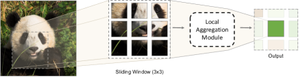
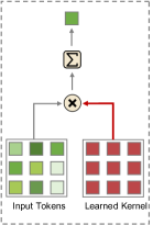
(a) Convolution

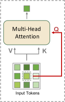
(b) SASA [49]

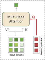
(c) QnA (ours)

Figure 2: QnA Overview. Local layers operate on images by considering overlapping windows (left), where the output is computed by aggregating information within each window: (a) Convolutions apply aggregation by learning weighted filters that are applied on each window. (b) Stand-Alone-Self-Attention (SASA) combines the window tokens via self-attention [49] — a time and memory consuming operation. (c) Instead of attending all window elements with each other, we employ learned queries that are shared across windows. This allows linear space complexity, while maintaining the expressive power of the attention mechanism.

3 Method

Query and Attend is a context-aware local feature processing layer. The key design choice of QnA is a convolution-like operation in which aggregation kernels vary according to the context of the processed local region. The heart of QnA is the attention mechanism, where overlapping windows are efficiently processed to maintain shift-invariance. Recall that three primary entities are deduced from the input features in self-attention: queries, keys, and values. The query-key dot product, which defines the attention weights, can be computationally pricey. To overcome this limitation, we detour from extracting the queries from the window itself but learn them instead (see Figure 2(c)). This process is conceptually similar to convolution kernels, as the learned queries determine how to aggregate token values, focusing on feature subspaces pre-defined by the network. We show that learning the queries maintains the expressive power of the self-attention mechanism and facilitates a novel efficient QnA implementation that uses only simple and fast operations. Finally, our layer can be extended to perform other functionalities (e.g., downsampling and upsampling), which are non-trivial in existing methods [49, 69].

Before the detailed explanation of QnA, we will briefly discuss the benefits and limitations of convolutions and self-attention. We let $H$ and $W$ be the height and width of the input feature maps, and denote $D$ as the embedding dimension. Otherwise, throughout this section, we use upper-case notation to denote a matrix or tensor entities, and lower-case notation to denote scalars or vectors.

3.1 Convolution

The convolution layer aggregates information by considering a local neighborhood of each element (e.g., a pixel) of the input feature $X\in\mathbb{R}^{H\times W\times D}$. Specifically, given a kernel $W\in\mathbb{R}^{k\times k\times D\times D}$, the convolution output at location $(i,j)$ is:

$$z_{i,j}=\sum_{\begin{subarray}{c}(n,m)\in\\ \mathcal{N}_{k}(i,j)\end{subarray}}x_{n,m}\cdot W_{\lfloor k/2\rfloor+i-n,\lfloor k/2\rfloor+j-m},$$ (1)

where the $k\times k$-spatial neighborhood of location $(i,j)$ is

$$\mathcal{N}_{k}(i,j)=\{(n,m)|-k/2<(i-n),(j-m)\leq k/2\}$$

(see Figure 2(a)). To simplify the notation, we omit $k$ from Equation 1 and re-write it in matrix notation as:

$$z_{i,j}=X_{\mathcal{N}_{i,j}}\cdot W,$$ (2)

For brevity, we assume a stride 1 for all strided operations, and padding is applied to maintain spatial consistency.

The number of convolutional parameters is quadratic in kernel size, inhibiting usage of large kernels, therefore limiting the ability to capture global interactions. In addition, reusing convolutional filters across different locations does not allow adaptive content-based filtering. Nevertheless, the locality and shift-invariance properties of convolutions benefit vision tasks. For this reason, convolutions are widely adopted in computer vision networks, and deep learning frameworks support hardware-accelerated implementation of Equation 1.

3.2 Self-Attention

A vision transformer network processes a sequence of $D$-dimensional vectors, $X\in\mathbb{R}^{N\times D}$, by mixing the sequence of size $N$ through the self-attention mechanism. These vectors usually encode some form of image patches where $N=H\times W$ and $H,W$ are the number of patches in each spatial dimension. Specifically, the input vectors are first projected into keys $K=XW_{K}$, values $V=XW_{V}$ and queries $Q=XW_{Q}$ via three linear projection matrices $W_{K},W_{V},W_{Q}\in\mathbb{R}^{D\times D}$. Then, the output of the self-attention operation is defined by:

$$\begin{split}\text{{SA}}(X)&=\text{{Attention}}\left(Q,K\right)\cdot V\\ &=\text{{Softmax}}\left(QK^{T}/{\sqrt{D}}\right)\cdot V,\end{split}$$ (3)

where $\text{{Attention}}\left(Q,K\right)$ is an attention score matrix of size $N\times N$ which is calculated using Softmax that is applied over each row.

Unlike convolutions, self-attention layers have a global receptive field and can process the whole input sequence, without affecting the number of learned parameters. Furthermore, every output of the self-attention layer is an input-dependent linear combination of the $V$ values, whereas in convolutions the aggregation is the same across the spatial dimension. However, the self-attention layer suffers from quadratic run-time complexity and inefficient memory usage, which makes it less favorable for processing high-resolution inputs. Furthermore, it has been shown that vanilla transformers don’t attend locally very well  [18, 65, 14, 56], which is a desired prior for downstream tasks. These models tend to become more local in nature only after a long and data-hungry training process [56].

3.3 Query-and-Attend

To devise a high-powered layer, we will adapt the self-attention mechanism into a convolution-like aggregation operation. The motivation behind this is that, as it has already been shown [13, 18], self-attention layer has better capacity than the convolution layer, yet, the inductive bias of convolutions allows better transferability and generalization capability [13]. Specifically, the locality and shift-invariance priors (for early stages) impose powerful guidance in the image domain.

We begin by revisiting the Stand-Alone-Self-Attention approach (SASA) [49], where attention is computed in small overlapping $k\times k$-windows, much like a convolution. The output $z_{i,j}$ of SASA is defined as:

$$z_{i,j}=\textbf{Attention}\left(q_{i,j},K_{\mathcal{N}_{i,j}}\right)\cdot V_{\mathcal{N}_{i,j}},$$ (4)

where $q_{i,j}=X_{i,j}W_{Q}$. In other words, in order to aggregate tokens locally, self-attention is applied between the tokens of each local window, and a single query is extracted from the window center (see Figure 2(b)).

While SASA [49] enjoy expressiveness and locality, through an input-adaptive convolution-like operation, it demands heavy memory usage. Specifically, to the best of our knowledge, all publicly available implementations use an unfolding operation that extracts patches from the input tensor. This operation expands the memory requirement by $k^{2}$ if implemented naively. Vaswani et al. [69] improved the memory-requirement of SASA [49] using local attention with halo expansion. Nevertheless, this implementation requires x3-x10 more memory than QnA while being x5-x8 slower, depending on $k$ (see Figure 3). This limitation makes the SASA layer infeasible for processing high-resolution images, employing larger kernels, or using sizable batches.

3.3.1 QnA - Single Query

To alleviate the compute limitation of SASA [49], we redefine the key-query dot product in Equation 4 by introducing learned queries. As we will later see, this modification leverages the weight-sharing principle (just like convolutions) and enables the efficient implementation of the QnA layer (see Section 3.4).

We begin by first replacing the queries $q_{i,j}$ from Equation 4 with a single $D$-dimensional vector $\tilde{q}$, that is learned during training. More particularly, we define the output of the QnA layer at location $(i,j)$ to be:

$$z_{i,j}=\textbf{Attention}\left(\tilde{q},K_{\mathcal{N}_{i,j}}\right)\cdot V_{\mathcal{N}_{i,j}}.$$ (5)

Through the above modification, we interpret the query-key dot product as the scalar-projection of the keys onto D-dimensional query directions. Therefore, the token values are aggregated according to their relative orientation with the query vectors. Intuitively, the keys can now be extracted such that relevant features’ keys will be closely aligned with $\tilde{q}$. This means that the network can optimize the query direction to detect contextually related features.

3.3.2 QnA - Multiple Queries

As it turns out, performance can be further pushed forward under our paradigm, with minimal computational overhead and negligible additional memory. The naive approach is to add channels or attention heads when considering multi-head attention. While this enhances expressiveness, additional heads induce a larger memory footprint and computational overhead. To improve the layer expressiveness, we can use $L$-different queries $\tilde{Q}\in\mathbb{R}^{L\times D}$ instead of one. Nevertheless, simply plugging in $\tilde{Q}$ in Equation 5 leads to $L\times D$ output, which expands the memory usage by $L$ (also known as cross-attention). Instead, we weight-sum the attention maps learned by the queries into a single attention map (for each attention head) and use it to aggregate the values. Therefore our QnA output becomes:

$$z_{i,j}=\left(\sum_{i\in\left[L\right]}\mathcal{W}_{i}*\textbf{Attention}\left(\tilde{Q}_{i},K_{\mathcal{N}_{i,j}}\right)\right)\cdot V_{\mathcal{N}_{i,j}},$$ (6)

where $\mathcal{W}\in\mathbb{R}^{L\times k^{2}}$ is a learned weight matrix, and $*$ is the element-wise multiplication operation. The overall extra space used in this case is $\mathcal{O}(L\times k^{2})$, which is relatively small, as opposed to the naive solution, which requires $\mathcal{O}(L\times D)$ extra space.

3.3.3 QnA Variants

Our layer naturally accommodates the improvements made for the vanilla self-attention layer [70]. Specifically, we use relative-positional embedding [55, 2, 32, 33, 76] and multi-head attention in all our models (further details can be found in Appendix F).

Upsampling & Downsampling Using QnA

down-sampling can be trivially attained using strided windows. To up-scale tokens by a factor $s$, we can use a QnA layer with $L=s^{2}$ learned queries. Assigning the result of each query as an entry in the upsampled output, we effectively construct a spatially dynamic upsampling kernel of size $s\times s$. We define the upsampling operation more formally in Appendix F. We show that QnA could be used to efficiently perform the upsampling function (Section 4.4) with improved performance, suggesting it can be incorporated into other vision tasks such as image synthesis.

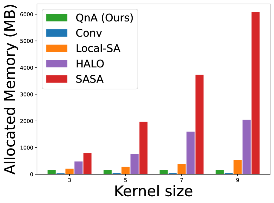
(a) Memory allocation

(b) Latency

Figure 3: Single Layer Computational Complexity During Forward Pass. QnA outperforms SASA [49], HaloNet [69], and local self-attention baselines in terms of speed and memory consumption. In particular, during forward pass, HaloNet [69] requires at least x3 additional memory allocation while being x5 slower. For larger kernels, the computation overhead becomes significant where up-to x10 additional memory allocation is needed. Convolutional layers are the most memory efficient, however they are x1.8 slower compared to QnA for large kernels. All experiments tested with PyTorch [51], on input size $256\times 256\times 64$.

3.4 Implementation & Complexity Analysis

The shared-learned queries across windows allow us to implement QnA using efficient operations that are available in existing deep-learning frameworks (e.g., Jax [4]). In particular, the query-key dot product can be calculated once on the whole input sequence, avoiding extra space allocation. Then, we can use window-based operations to effectively calculate the softmax operation over the overlapping windows, leading to a linear time-and-space complexity (see Figure 3). Full-implementation details of our method are in Appendix D, along with a code snippet in Jax/Flax [4, 29].

3.5 The QnA-ViT Architecture

The QnA-ViT architecture is composed of vision transformer blocks [18] (for global context) and QnA blocks (for local context). The QnA block shares a similar structure with the ViT block, except we replace the multi-head self-attention layer with the QnA layer. We present a family of architectures that follow the design of ResNet [28]. Specifically, we use a 4-stage hierarchical architecture. The base dimension $D$ varies according to the model size. Below we indicate how many layers we use in each stage ($T$ stands for ViT-blocks and $Q$ stands for QnA-blocks):

• Tiny: $D,T,Q\!=\{64,\left[0,0,4,2\right],\left[3,4,3,0\right]\}$

• Small: $D,T,Q\!=\{64,\left[0,0,12,2\right],\left[3,4,7,0\right]\}$

• Base: $D,T,Q\!=\{96,\left[0,0,12,2\right],\left[3,4,7,0\right]\}$

For further details, please refer to Appendix C.

4 Experiments

4.1 Image Recognition & ImageNet-1K Results

Method	Params	GFLOPS	Throughput	Top-1 Acc.
ResNet50 [28, 74]	26M	4.1	1287	80.4
ResNet101 [28, 74]	45M	7.9	770	81.5
ResNet152 [28, 74]	60M	11.6	539	82.0
DeiT-S [65]	22M	4.6	940	79.8
DeiT-B [65]	86M	17.5	292	81.8
Swin-Tiny [45]	29M	4.5	723	81.3
Swin-Small [45]	50M	8.7	425	83.0
Swin-Base [45]	88M	15.4	277	83.5
Swin-Base [45]${\scriptstyle\uparrow 384}$	88M	47.0	85	84.5
NestT-Tiny [89]	17M	5.8	568	81.5
NestT-Small [89]	38M	10.4	352	83.3
NestT-Base [89]	68M	17.9	233	83.8
Focal-Tiny [45]	29M	4.9	546	82.2
Focal-Small [45]	51M	9.1	282	83.5
Focal-Base [45]	90M	16.0	207	83.8
QnA-Tiny	16M	2.5	1060	81.7
QnA-Tiny${\scriptstyle 7\times 7}$	16M	2.6	895	82.0
QnA-Small	25M	4.4	596	83.2
QnA-Base	56M	9.7	372	83.7
QnA-Base${\scriptstyle\uparrow 384}$	56M	30.6	177	84.8

Table 1: ImageNet-1K[58] pre-training results. All models were pre-trained and tested on input size $224\times 224$. Models marked with $\uparrow 384$ are later also fine-tuned and tested on $384^{2}$ resolution, following [67]. The Accuracy, parameter count, and floating point operations are as reported in the corresponding publication. Throughput was calculated using the timm [73] library, on a single NVIDIA V100 GPU with 16GB memory. For QnA${\scriptstyle 7\times 7}$, a $7\times 7$ window size was used instead of $3\times 3$. Our model achieves comparable results to state-of-the-art models, with fewer parameters and better computation complexity.

Setting:

we evaluate our method using the ImageNet-1K [58] benchmark, and follow the training recipe of DEiT [65], except we omit EMA [53] and repeated augmentations [31]. For full-training details please refer to Appendix B.

Results:

A summary comparison between different models appears in Table 1. As shown from the table, most transformer-based vision models outperform CNN-based ones in terms of the top-1 accuracy, even when the CNN models are trained using a strong training procedure. For example, ResNet50 [28] with standard ImageNet training achieves 76.6% top-1 accuracy. However, as argued in [74], with better training, its accuracy sky-rockets to 80.4%. Indeed, this is a very impressive improvement, yet it falls short behind transformer models. In particular, our model (the tiny version) improves upon ResNet by 1.3% with  40% fewer parameters and FLOPs.

In terms of speed, CNNs are very fast and have a smaller memory footprint (see Figure 3). The throughput gap can be evident by investigating the vision transformers reported in Table 1. A particular strong ViT is the Focal-ViT [82]; in its tiny version, it improves upon ResNet101 by 0.7% while the latter enjoys x1.4-times better throughput. Nonetheless, our model stands out in terms of the speed-accuracy trade-off. Comparing QnA-Tiny with Focal-Tiny, we achieve only 0.5% less accuracy while having x2-times better throughput, parameter-count, and flops. We can even reduce this gap by training the QnA with a larger receptive field. For example, setting the receptive field of the QnA to be 7x7, instead of 3x3, achieve 82.0% accuracy, with negligible effect on the model speed and size.

Finally, we notice that most Vision Transformers achieve similar Top-1 accuracy. More specifically, tiny models (in terms of parameters and number of FLOPs) achieve roughly the same Top-1 accuracy of 81.2-82.0%. The accuracy difference is even less significant in larger models (e.g., base variants accuracy differs by only 0.1%), and this accuracy difference can be easily tipped to either side by many factors, even by choosing a different seed [52]. Nonetheless, our model is faster, all while using fewer resources.

The reason behind better accuracy-efficiency trade-off:

QnA-ViT achieves a better accuracy-efficiency trade-off for several reasons. First, QnA is fast, which is crucial for better throughput. Further, most of the vision transformer’s parameter count is due to the linear projection matrices. Our method reduces the number of linear projections by omitting the query projections (i.e., the $W_{q}$ matrix is replaced with 2-learned queries). Furthermore, the feed-forward network requires $\times 2$ more parameters than the self-attention. Our model uses smaller embedding dimensions than existing models without sacrificing accuracy. Namely, NesT-Tiny [89] uses an embedding dimension of 192, while Swin-Tiny [45] and Focal-Tiny [82] use 96 embedding dimensions. On the other hand, our method achieves a similar feature representation capacity, with a lower dimension of 64.

Finally, other parameter efficient methods achieve low parameter count by training on larger input images [69, 64]. This is shown to improve image-classification accuracy [67]. However, it comes at the cost of lower-throughput and more FLOPs. For example, EfficientNet-B5 [64], which was trained and tested on images of $456\times 456$ resolution, achieves 83.6% accuracy while using only 30M parameters. Nonetheless, the network’s throughput is 170 images/sec, and it uses 9.9 GFLOPs. Compared to our base model, QnA achieves similar accuracy with twice the throughput. Also, it is important to note that these models were optimized via Neural Architecture search, an automated method for better architecture design. We believe employing methods with similar purpose [81] would even further optimize our models’ parameter count.

		QnA
	SASA	$L=1$	$L=2$	$L=3$	$L=4$
Top-1 Acc.	80.86	80.3	80.7	80.76	80.81
Params (M).	16.440	16.182	16.188	16.192	16.200.
FLOPS (G)	2.620	2.378	2.400	2.420	2.442

Table 2: Multiple queries effect. We compare the performance of SASA [49] to QnA with a varying amount of queries. As can be seen, using multiple queries improves QnA, reaching comparable performance, using an order of magnitude less memory.

4.2 Ablation & Design Choices

Number of Queries:

Using multiple queries allows us to capture different feature subspaces. We consider SASA [49] as our baseline, which extracts the self-attention queries from the window elements. Due to its heavy memory footprint, we cannot consider SASA variants similar to QnA-ViT. Instead, we consider a lightweight variant that combines local self-attention with SASA. All SASA layers use a 3x3 window size. Downsampling is performed similar to QnA-ViT, except that we replace QnA with SASA. Finally, the local-self attention layers use a 7x7 window size without overlapping (see Section E.1). The results are summarized in Table 2. As can be seen, we achieved comparable results to SASA. In addition, two queries outperform one, but this improvement saturates quickly. We hence recommend using two queries, as it enjoys efficiency and expressiveness.

Number of heads:

Most vision transformers use large head dimension (e.g., $\geq 32$)[66]. However, we found that the QnA layer enjoys more heads. We trained various models based on QnA and self-attention layers with different training setups to verify this. Our experiments found that a head dimension $d=8$ works best for QnA layers. Similar to previous work [66], in hybrid models, where both self-attention and QnA layers are used, we found that self-attention layers still require a large head dimension (i.e., $d=32$). Moreover, we found that using more heads for QnA is considerably better (up to $1\%$ improvement) for small networks. Moreover, this performance gap is more apparent when training the models for fewer epochs without strong augmentations (see Section E.2 for further details). Intuitively, since the QnA layer is local, it benefits more from local pattern identifications, unlike global context, which requires expressive representation.

Global Attention	QnA	Downsampling	Params	FLOPs	Top1-Acc.
Different downsampling choices
[3,3,6,2]	[0,0,0,0]	Nest [89]	16.8M	3.7	81.2
[3,3,6,2]	[0,0,0,0]	Swin [45]	16.0M	3.1	81.2
[3,3,6,2]	[1,1,1,0]	QnA	16.0M	3.2	81.9
Number of QnA blocks vs Transformer blocks
[0,0,0,0]	[4,4,7,2]	QnA	14.9M	2.4	80.9
[3,3,6,2]	[1,1,1,0]	QnA	16.0M	3.2	81.9
[0,0,4,2]	[4,4,3,0]	QnA	15.8M	2.6	81.9
Deeper Models
[0,0,8,2]	[3,4,11,0]	QnA	24.7M	4.2	82.7
[0,0,10,2]	[3,4,9,0]	QnA	24.8M	4.3	83.0
[0,0,12,2]	[3,4,7,0]	QnA	25.0M	4.4	83.2
[0,0,16,2]	[3,4,3,0]	QnA	25.3M	4.6	83.1

Table 3: Ablation studies and design choices. In the first two columns we specify the number of global-attention and QnA layers used in each stage. See Section 4.2 for further details, and the supp. materials for more configurations.

How many QnA layers do you need?

In order to verify the expressive power of QnA, we consider a dozen different models. Each model consists of four stages. In each stage, we consider using self-attention and QnA layers. A summary report can be found in Table 3 (for the full report, please see Section E.3). In our experiments, we conclude that the QnA layer is effective in the early stages and can replace global attention without affecting the model’s performance. QnA is fast and improves the model’s efficiency. Finally, the QnA layer is a very effective down-sampling layer. For example, we considered two baseline architectures which are mostly composed of transformer blocks, (1) one model uses simple 2x2 strided-convolution to reduce the feature maps (adopted in [45]), and the (2) other is based on the down-sampling used in NesT [89], which is a 3x3 convolution, followed by a layer-norm and max-pooling layer. These two models achieve similar accuracy, which is 81.2%. On the other hand, when merely replacing the downsampling layers with the QnA layer, we witness a  0.7% improvement without increasing the parameter count and FLOPs. Note, global self-attention is still needed to achieve good performance. However, it can be diminished by local operations, e.g., QnA.

Deep models:

To scale-up our model, we chose to increase the number of layers in the network’s third stage (as typical in previous works [28]). This design choice is adapted mainly for efficiency reasons, where the spatial and feature dimension are manageable in the third stage. In particular, we increase the total number of layers in the third stage from 7 to 19 and consider four configurations where each configuration varies by the number of QnA layers used. The models’ accuracies are reported in Table 3. As seen from the table, the model’s accuracy can be maintained by reducing the number of global attention. This indicates that while self-attention can capture global information, it is beneficial to a certain degree, and local attention could be imposed by the architecture design for efficiency consideration.

4.3 Object Detection

Model	Backbone	$\text{AP}_{\text{50}}$	$\text{AP}_{\text{75}}$	$\text{AP}_{\text{L}}$	$\text{AP}_{\text{M}}$	$\text{AP}_{\text{S}}$	AP
	R50	55.4	36.6	53.2	38.0	15.1	35.3
DETR	QnA-Ti	58.9	38.6	56.8	40.6	16.0	37.5
	QnA-Ti7	59.6	39.3	57.6	41.2	16.0	37.9
DETR-QnA	QnA-Ti	59.6	39.7	57.4	41.8	18.2	38.5

Table 4: DETR [7] Based Object detection on the COCO Dataset [44]. Incorporating QnA-ViT-Tiny with DETR substantially improves upon the ResNet50 backbone (by up to 3.2). QnA with receptive field 7x7 improves the average precision on large objects ($\text{AP}_{\text{L}}$), and incorporating QnA into the DETR network improves performance on smaller objects, indicating locality.

Setting:

To evaluate the representation quality of our pre-trained networks, we use the DETR [7] framework, which is a transformer-based end-to-end object detection framework. We use three backbones for our evaluations; ResNet50 [28], and two variants of QnA-ViT, namely, QnA-ViT-Tiny, and QnA-ViT-Tiny-7x7, which uses a 7x7 receptive for all QnA layers (instead of 3x3). Complete training details are provided in the supplemental material.

Revisiting DETR transformer design:

DETR achieves comparable results to CNN-based frameworks [57]. However, it achieves less favorable average precision when tested on smaller objects. The DETR model uses a vanilla transformer encoder to process the input features extracted from the backbone network. As argued earlier, global attention suffers from locality issues. To showcase the potential of incorporating QnA in existing transformer-based networks, we propose DETR-QnA architecture, in which two transformer blocks are replaced with four QnA blocks.

Results:

We report the results in Table 4. As can be seen, DETR trained with QnA-Tiny achieves +2.2 better AP compared to the ResNet50 backbone. Using a larger receptive field ($7\times 7$) further improves the AP by 0.4. However, much improvement is due to better performance on large objects (+0.7). Finally, when incorporating QnA into the DETR encoder, we gain an additional +0.6AP (and +1.0AP relative to using the DETR model). More particularly, incorporating QnA with DETR achieves an impressive +2.2 AP improvement on small objects, indicating the benefits of QnA’s locality.

(a) Bilinear

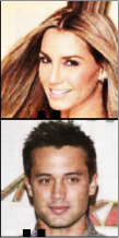
(b) ConvTransposed

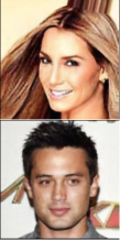
(c) QnA

Figure 4: Qualitative Auto-Encoder Results. We train a simple Autoencoder using convolution layers (a-b), and (c) QnA layers. We show reconstructed images from the CelebA test set [46]. QnA shows preferable reconstructions. See Section 4.4 for more details.

4.4 QnA as an upsampling layer

We suggest that QnA can be adapted to other tasks besides classification and detection. To demonstrate this, we train an autoencoder network on the CelebA [46] dataset, using the $L_{1}$ reconstruction loss. We consider two simple baselines that are convolution-based. In particular, one baseline uses bilinear up-sampling to upscale the feature maps, and another baseline uses the transposed convolution layer [86]. Qualitative and quantitative results appear in Figure 4 and Figure 5, respectively. The figures show that the QnA-based auto-encoder achieves better qualitative and quantitative results and introduces fewer artifacts (see Appendix G for further details).

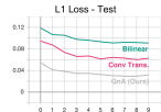
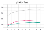
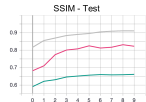
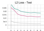
Figure 5: Quantitative Auto-Encoder Results are reported, compared to the same convolutional baselines as in Figure 4. We compare our method (gray) to bilinear upsampling (green) and transposed covolution-based upsampling (pink). We show consistent improvement across epochs (horizontal axes) in the L1 loss (top left), the pSNR (top right), the SSIM (bottom left), and MSE (bottom right) metrics.

5 Limitations & Conclusion

We have presented QnA, a novel local-attention layer with linear complexity that is also shift-invariant. Through rigorous experiments, we showed that QnA could serve as a general-purpose layer and improve the efficiency of vision transformers without compromising on the accuracy part. Furthermore, we evaluated our method in the object-detection setting and improved upon the existing self-attention-based method. Our layer could also be used as an up-sampling layer, which we believe is essential for incorporating transformers in other tasks, such as image generation. Finally, since QnA is attention-based, it requires additional intermediate memory, whereas convolutions operate seamlessly, requiring no additional allocation. Nonetheless, QnA has more expressive power than convolution. In addition, global self-attention blocks are more powerful in capturing global context. Therefore, we believe that our layer mitigates the gap between self-attention and convolutions and that future works should incorporate all three layers to achieve the best performance networks.

Appendix A Attention Visualization

In QnA, the aggregation kernel of each window is derived from the attention scores between the learned queries and the window keys. To visualize the attention of the whole image, we choose to sum the scores of each spatial-location as obtained in all relevant windows. You can find the visualization in Figure 6. As shown in Figure 6, the attentions are content-aware, suggesting the window aggregation kernels are spatially adaptive. For the learned kernels in each window, please refer to Figure 7.

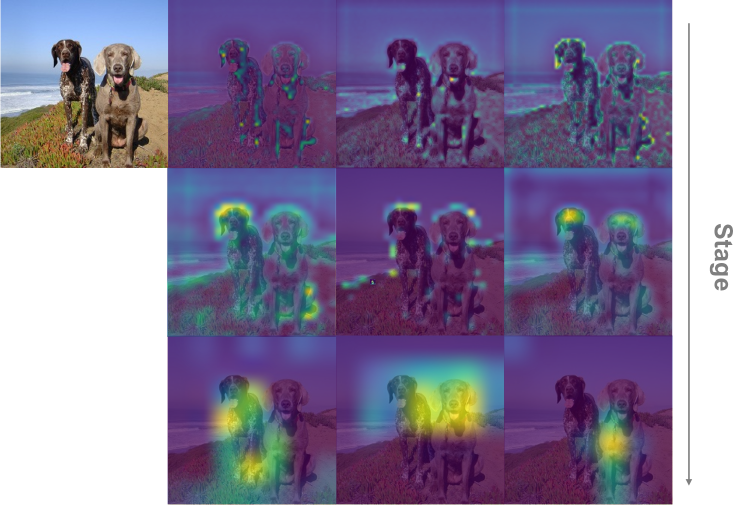
Figure 6: QnA attention visualization of different heads. To visualize a specific location’s attention score, we sum the attention scores obtained for that location in all windows. Attention maps are up-sampled and overlaid on the image for better visualization.

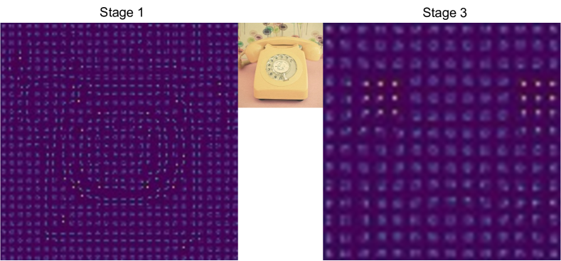
Figure 7: QnA aggregation kernels visualization. The attention kernels are tiled in the visualization instead of overlapped, causing the uniform grid effect. Brighter areas indicate higher attention scores. (best viewed when zoomed-in).

Appendix B Full training details

B.1 Image Classification

We evaluate our method using the ImageNet-1K [58] benchmark, which contains 1.28M training images and 50,000 validation images from 1,000 classes. We follow the training recipe of DEiT [65], except we omit EMA [53] and repeated augmentations [31]. Particularly, we train all models for 300-epochs, using the AdmaW [40, 48] optimizer. We employ a linearly scaled learning rate $lr=\texttt{5e-4}\cdot\frac{\text{Batch size}}{256}$ [24], with warmup epochs [47] varying according to model size and weight decay $wd=\texttt{5e-2}$. For augmentations, we apply RandAugment [12], mixup [87] and CutMix [85] with label-smoothing [84], and color-jitter [9]. Finally, an increasing stochastic depth is applied [36]. Note this training recipe (with minor discrepancy between previous papers), is becoming the standard when training a Vision Transformer on the ImageNet benchmark. Finally, we normalize the queries in all QnA layers to be unit-vectors for better training stability.

B.2 Object Detection

We train the DETR model on COCO 2017 detection dataset [44], containing $118K$ training images and a $5k$ validation set size. We utilize the training setting of DETR, in which the input is resized such that the shorter side is between 480 and 800 while the longer side is at most 1333 [77]. An initial learning rate of $\mathtt{1e-4}$ is set for the detection transformer, and $\mathtt{1e-5}$ learning rate for the backbone network. Due to computational limitations, we use a short training scheduler of 75 epochs with a batch size of 32. The learning rates are scaled by 0.1 after 50 epochs. We trained DETR using the implementation in [16].

Appendix C QnA-ViT architecture

The QnA-ViT architecture is composed of transformer blocks [18] and QnA blocks. First we split the image into $4\times 4$ patches, and project them to form the input tokens. The vision transformer block is composed of a multihead attention layer (MSA) and an inverted-bottleneck feed forward network (FFN), with expansion 4. The output of block-$l$ is:

$$\begin{split}&z^{\prime}_{l}=\mathbf{MSA}\left(\mathbf{LayerNorm}(z_{l-1})\right)+z_{l-1}\\ &z_{l}=\mathbf{FFN}\left(\mathbf{LayerNorm}(z^{\prime}_{l})\right)+z^{\prime}_{l}.\end{split}$$

The QnA block shares a similar structure, except we replace the MSA layer with QnA layer. Downampling is performed using QnA blocks with stride set to 2 (to enable skip-connections we use $1\times 1$-convolution with similar stride). We employ pre-normalization [80] to stabilize training. Finally, we use global average pooling [43] right before the classification head, with LayerNorm [1] employed prior to the pooling operation. Full architecture details can be found in Table 5.

Stage	Output	QnA-T		QnA-S		QnA-B
		QnA Blocks	SA Blocks	QnA Blocks	SA Blocks	QnA Blocks	SA Blocks
1	56x56	4x4 Conv, stride 4, dim 64		4x4 Conv, stride 4, dim 64		4x4 Conv, stride 4, dim 96
		$\begin{bmatrix}\text{3x3 QnA-Block,}\\ \text{stride 1,}\\ \text{head 8}\end{bmatrix}\times 2$	None	$\begin{bmatrix}\text{3x3 QnA-Block,}\\ \text{stride 1,}\\ \text{head 8}\end{bmatrix}\times 2$	None	$\begin{bmatrix}\text{3x3 QnA-Block,}\\ \text{stride 1,}\\ \text{head 6}\end{bmatrix}\times 2$	None
2	28x28	3x3 QnA, stride 2, head 16, dim 128		3x3 QnA, stride 2, head 16, dim 128		3x3 QnA, stride 2, head 16, dim 192
		$\begin{bmatrix}\text{3x3 QnA-Block,}\\ \text{stride 1,}\\ \text{head 16}\end{bmatrix}\times 3$	None	$\begin{bmatrix}\text{3x3 QnA-Block,}\\ \text{stride 1,}\\ \text{head 16}\end{bmatrix}\times 3$	None	$\begin{bmatrix}\text{3x3 QnA-Block,}\\ \text{stride 1,}\\ \text{head 12}\end{bmatrix}\times 3$	None
3	14x14	3x3 QnA, stride 2, head 32, dim 256		3x3 QnA, stride 2, head 32, dim 256		3x3 QnA, stride 2, head 32, dim 384
		$\begin{bmatrix}\text{3x3 QnA-Block,}\\ \text{stride 1,}\\ \text{head 32}\end{bmatrix}\times 2$	$\begin{bmatrix}\text{SA-Block,}\\ \text{win sz. 14 x 14,}\\ \text{head 8}\end{bmatrix}\times 4$	$\begin{bmatrix}\text{3x3 QnA-Block,}\\ \text{stride 1,}\\ \text{head 32}\end{bmatrix}\times 6$	$\begin{bmatrix}\text{SA-Block,}\\ \text{win sz. 14 x 14,}\\ \text{head 8}\end{bmatrix}\times 12$	$\begin{bmatrix}\text{3x3 QnA-Block,}\\ \text{stride 1,}\\ \text{head 24}\end{bmatrix}\times 6$	$\begin{bmatrix}\text{SA-Block,}\\ \text{win sz. 14 x 14,}\\ \text{head 12}\end{bmatrix}\times 12$
4	7x7	3x3 QnA, stride 2, head 64, dim 512		3x3 QnA, stride 2, head 64, dim 512		3x3 QnA, stride 2, head 48, dim 768
		None	$\begin{bmatrix}\text{SA-Block,}\\ \text{win sz. 7 x 7,}\\ \text{head 16}\end{bmatrix}\times 2$	None	$\begin{bmatrix}\text{SA-Block,}\\ \text{win sz. 7 x 7,}\\ \text{head 16}\end{bmatrix}\times 2$	None	$\begin{bmatrix}\text{SA-Block,}\\ \text{win sz. 7 x 7,}\\ \text{head 24}\end{bmatrix}\times 2$

Table 5: QnA-ViT architecture details. QnA is used to down-sample the feature maps between two consecutive stages. In stage 3 we first employ global self-attention blocks.

Appendix D Implementation & complexity - extended

In this section we provide full details on the efficient implementation of QnA. To simplify the discussion, we only consider a single-query without positional embedding.

Let us first examine the output of a QnA layer, by expanding the softmax operation inside the attention layer:

$$\begin{split}z_{i,j}&=\textbf{Attention}\left(\tilde{q},K_{\mathcal{N}_{i,j}}\right)\cdot V_{\mathcal{N}_{i,j}}\\ &=\frac{\sum_{\mathcal{N}_{i,j}}e^{\tilde{q}K_{n,m}}v_{n,m}}{\sum_{\mathcal{N}_{i,j}}e^{\tilde{q}K_{n,m}}}.\end{split}$$

Recall, $\mathcal{N}_{i,j}$ is the $k\times k$-window at location $(i,j)$. While it may seem that we need to calculate the query-key dot product for each window, notice that since we use the same query over each window, then we can calculate $\tilde{q}K^{T}$ once for the entire input. Also, we can leverage the matrix multiplication associativity and improve the computation complexity by calculating $\tilde{q}W_{k}^{T}$ first (this fused implementation reduces the memory by avoiding the allocation of the key entities). Once we calculate the query-key dot product, we can efficiently aggregate the dot products using the sum-reduce operation supported in many deep learning frameworks (e.g., Jax [4]). More specifically, let $\mathbf{Sum}_{k}(\dots)$ be a function that sums-up values in each $k\times k$-window, then:

$$z_{i,j}=\frac{\sum_{\mathcal{N}_{i,j}}e^{\tilde{q}K_{n,m}}v_{n,m}}{\sum_{\mathcal{N}_{i,j}}e^{\tilde{q}K_{n,m}}}=\frac{\mathbf{Sum}_{k}\left(e^{\tilde{q}K^{T}}*V\right)}{\mathbf{Sum}_{k}\left(e^{\tilde{q}K^{T}}\right)},$$

where * is the element wise multiplication. A pseudo-code of our method can be found in Algorithm 1. We further provide a code-snippet of the QnA module, implemented in Jax/Flax [5, 30] (see Figure 8).

Complexity Analysis:

in the single query variant, extracting the values and computing the key-query dot product require $2HWD^{2}$ computation and $HW+HWD$ extra space. Additionally, computing the softmax using the above method requires additional $\mathcal{O}(k^{2}HWD)$ computation (for summation and division), and $\mathcal{O}(HWD)$ space (which is independent of $k$, i.e., the window size). For multiple-queries variant ($L=2$), see empirical comparison in Fig. 3.

⬇

1class QnA(nn.Module):

2 @nn.compact

3 def __call__(self, X):

4 # Initialize Parameters:

5 Q = # Query vectors [L, h, D//h]

6 Wk = # Linear Projection for keys [D, D]

7 Ws = # Attention weight scale [k, k, L * h]

8 B_rpe = #Relative PE [k, k, L * h]

9 # Fused implementation of Q*(X*W_K).Transpose

10 Wk = Wk.reshape([-1, heads, D // heads])

11 QWk = jnp.einsum(’lhd,Dhd->Dlh’, Q, Wk)

12 QK_similariy = jnp.einsum(’BHWD,BDqh->BHWqh’, X, QWk)

13 # Compute V

14 V = nn.Dense(D)(X).reshape([B, H, W, heads, D // heads])

15 # Compute Attention:

16 exp_similarity = jnp.exp(QK_similariy) # [B, H, W, L, h]

17 exp_similarity_v = exp_similarity[..., jnp.newaxis] * V[:,:,: jnp.newaxis,:] # [B, H, W, L, D]

18 aux_kernel = (jnp.exp(B_rpe) * Ws).repeat(repeats=D // heads, axis=-1) # [k, k, d, L*h]

19 A = jax.lax.conv_general_dilated(exp_similarity_v.reshape([B, H, W, LD]),

20 aux_kernel, window_strides=[s, s], padding=’SAME’,

21 feature_group_count=L * D,).reshape([B, H_out, W_out, L, heads, D // heads])

22 A = jnp.reshape(A, [B, H_out, W_out, L, heads, D // heads])

23 aux_kernel = jnp.exp(B_rpe) # [k, k, 1, L*h]

24 B = jax.lax.conv_general_dilated(exp_similarity.reshape([B, H, W, -1]),

25 aux_kernel,

26 window_strides=[s, s],

27 padding=’SAME’,

28 dimension_numbers=_conv_dimension_numbers(I.shape)

29 ).reshape([B, H_out, W_out, L, heads, 1])

30 out_heads = jnp.sum(A / B, axis=-2).reshape([B, H_out, W_out, D])

31 final_out = nn.Dense(self.D)(out_heads)

32 return final_out

Figure 8: Code snippet of the QnA module implemented in Jax [5] and Flax [30]. Full implementation, with pre-trained networks weights, will be made publicly available.

Algorithm 1 Efficient implementation of QnA. All operations can be implemented efficiently with little memory-overhead. Further, $\mathbf{Sum}_{k}$ applies sum-reduction to all elements in each $k\times k$-window.

1:$X\in\mathbb{R}^{H\times W\times D}$

2:$W_{K},W_{V}\in\mathbb{R}^{D\times D}$, $\tilde{q}\in\mathbb{R}^{D}$

3:// Compute values:

4:     $V\leftarrow XW_{V}$

5:// Compute the query-key dot product ( $\mathbf{S\leftarrow\tilde{q}K^{T}}$):

6:     Let $A\leftarrow\tilde{q}W_{K}^{T}$

7:     for $l\in\left[L\right],i,j\in\left[H\right]\times\left[W\right]$ do

8:         $S_{l,i,j}\leftarrow A_{l,i,j}\cdot X_{i,j}^{T}$

9:     end for

10:// Compute the final output:

11:     Let $B\leftarrow e^{S}$ be the element-wise exponent of $S$

12:     Let $C\leftarrow B*V$ $\triangleright$ $*$ is the element-wise product

13:     return $\mathbf{Sum}_{k}(C)/\mathbf{Sum}_{k}(B)$

Appendix E Design choices - full report

E.1 Number of queries

To verify the effectiveness of using multiple queries, we trained a lightweight QnA-ViT network composed of local self-attention blocks and QnA blocks. We set the window size of all local self-attention layers to be 7x7, and we use a 3x3 receptive field for QnA layers. All the downsampling performed are QnA-Based. A similar architecture was used for the SASA [49] baseline, where we replaced the QnA layers with SASA layers. The number of QnA/SASA blocks used for each stage are ${[}2,2,2,0{]}$ and the number of local self-attention blocks are ${[}1,1,5,2{]}$.

E.2 Number of heads

Using more attention heads is beneficial for QnA. More specifically, we conducted two experiments, one where we use only QnA blocks and the second where we use both QnA blocks and (global) self-attention blocks. In the first experiment, we use the standard ImageNet training preprocessing [63], meaning we employ random crop with resize and random horizontal flip. In the second experiment, we used DeiT training preprocessing. We show the full report in Table 6 and Table 7.

First, from Table 6, we notice that training shallow QnA-networks for fewer epochs requires many attention heads. Furthermore, it is better to maintain a fixed dimension head across stages - this is done by doubling the number of heads between two consecutive stages. For deeper networks, the advantage of using more heads becomes less significant. This is because the network can capture more feature subspaces by leveraging its additional layers. Finally, when using both QnA and ViT blocks, it is still best to use more heads for QnA layers, while for ViT blocks, it is best to use a high dimension representation by having fewer heads (see Table 7).

QnA Blocks	Heads	AugReg	Epochs	Top-1 Acc.
[2,2,2,2]	[2,2,2,2]	None	90	68.33
	[4,4,4,4]			69.05
	[8,8,8,8]			69.98
	[2,4,8,16]			70.08
	[4,8,16,32]			70.54
	[8,16,32,64]			71.12
[3,4,6,3]	[2,4,8,16]	None	90	72.66
	[4,8,16,32]			72.82
	[8,16,32,64]			73.02

Table 6: The affect of number of heads on QnA. We train two networks using the Inception preprocessing [63], i.e., random crop and horizontal flip. We set the number of QnA blocks according to the ResNet-18 and ResNet-50 networks (the number of blocks for each stage is stated in the first column). As can be seen, using fixed head-dimension is better than increasing the head-dimension as we propagate through the network. Shallow networks benefit from having many heads, while deeper networks gain less from more heads. Therefore we suggest increasing the head-dimension for deeper networks for better memory utilization.

Blocks		Heads		AugReg	Epochs	Top-1 Acc.
QnA	SA	QnA	SA
[1,2,3,0]	[1,1,3,2]	[2,4,8,16]	[2,4,8,16]	DeiT [65]	90	78.17
		[4,8,16,32]	[4,8,16,32]			79.24
		[8,16,32,64]	[8,16,32,64]			79.34
		[8,16,32,64]	[2,4,8,16]			79.31
		[8,16,32,64]	[4,8,16,32]			79.53
[1,2,3,0]	[1,1,3,2]	[8,16,32,64]	[2,4,8,16]	DeiT [65]	300	81.5
		[8,16,32,64]	[4,8,16,32]			81.49

Table 7: The number of heads affect on QnA and ViT Blocks. QnA still benefits from more heads, while ViT blocks need higher-dimension representation, specially for longer training.

E.3 How many QnA layers do you need?

To understand the benefit of using QnA layers, we consider a dozen network architectures that combine vanilla ViT and QnA blocks. For ViT blocks, we tried to use global attention in the early stages but found it better to use local self-attention and restrict the window size to be at most 14x14. We group the architecture choices into three groups:

1. We consider varying the number of QnA blocks in the early stages.

2. We change the number of QnA blocks in the third stage.

3. We use lower window size for the local-self attention blocks. Namely, 7x7 window in all ViT blocks at all stages.

Finally, all networks were trained for 300 epochs following DeiT preprocessing. The full report can be found in Table 8.

From Table 8, local-self attention is not very beneficial in the early stages and can be omitted by using QnA blocks only. Furthermore, using more global-attention blocks in deeper stages is better, but the network’s latency can be reduced by having a considerable amount of QnA blocks. Finally, local self-attention becomes less effective when using a lower window size. In particular, since QnA is shift-invariant, it can mitigate the lack of cross-window interactions, reflected in the improvement gain we achieve when using more QnA blocks.

Blocks		Params	GFLOPS	Top- Acc
QnA	SA
Changes in stages 1, 2
[1,1,4,0]	[3,3,3,2]	16.62M	3.200	81.70
[2,2,4,0]	[2,2,3,2]	16.51M	2.909	81.74
[3,3,4,0]	[1,1,3,2]	16.40M	2.875	81.86
[4,4,4,0]	[0,0,3,2]	16.30M	2.584	81.83
Changes in stage 3
[4,4,7,0]	[0,0,0,2]	16.00M	2.631	80.8
[4,4,5,0]	[0,0,2,2]	16.25M	2.698	81.30
[4,4,3,0]	[0,0,4,2]	16.40M	2.628	81.9
[4,4,1,0]	[0,0,6,2]	16.55M	2.714	81.9
Local SA with window size $7\times 7$
[1,1,1,0]	[2,2,6,2]	16.38M	2.568	80.0
[2,2,2,0]	[1,1,5,2]	16.3M	2.491	80.6
[2,2,3,0]	[1,1,4 ,2]	16.23M	2.471	80.7
[2,2,4,0]	[1,1,3, 2]	16.16M	2.450	80.8

Table 8: How much QnA do you really need? - full report. The number of QnA and local self-attention (SA) blocks in each stage are indicated in the first row. In the first two sub-tables, a window size of $14\times 14$ except in the last stage, where a $7\times 7$ window size was set. In the last sub-table, we reduce the window size to become $7\times 7$ for all stages.

Appendix F QnA Variants - extended version

As discussed in the paper, we incorporate multi-head attention and positional embedding in our layer.

Positional Embedding

Self-attention is a permutation invariant operation, meaning it does not assume any spatial relations between the input tokens. This property is not desirable in image processing, where relative context is essential. Position encoding can be injected into the self-attention mechanism to solve this. Following recent literature, we use relative-positional embedding [55, 2, 32, 33, 76]. This introduces a spatial bias into the attention scheme, rendering Eq. 3 (from the main text) now to be:

$$\textbf{Attention}\left(Q,K\right)=\textbf{Softmax}\left(QK^{T}/{\sqrt{D}}+B\right),$$ (7)

where $B\in\mathbb{R}^{k\times k}$ is a learned relative positional encoding. Note, different biases are learned for each query in the QnA layer, which adds $\mathcal{O}(L\times k^{2})$ additional space.

Multi-head attention:

As in the original self-attention layer [70], we use multiple heads in order to allow the QnA layer to capture different features simultaneously. In fact, as we will show in Section E.2, using more attention heads is beneficial to QnA.

In mutli-head attention, all queries $Q$, keys $K$, and values $V$ entities are split into $h$ sub-tensors, which will correspond to vectors in the lower dimensional space $\mathbb{R}^{D/h}$. More specifically, let $Q^{(i)},K^{(i)},V^{(i)}$ be the $i$-th sub vector of each query, key and value, respectively. The self-attention of head-$i$ becomes:

$$\begin{split}\text{head}_{i}&=\textbf{Attention}\left(Q^{(i)},K^{(i)}\right)V^{(i)}\\ &=\textbf{Softmax}\left(Q^{(i)}K^{(i)T}/{\sqrt{d_{h}}}+B\right)V^{(i)},\end{split}$$ (8)

, where $d_{h}=D/h$, and the output of the Multi-Head Attention (MHA) is:

$$\begin{split}\textbf{MHA}&\left(Q,K,V\right)=\\ &\texttt{Concat}\left(\text{head}_{1},\dots,\text{head}_{h}\right)W_{O}\end{split}$$ (9)

, where $W_{O}\in\mathbb{R}^{D\times D}$ is the final projection matrix.

Up-sampling using QnA

Up-sampling by factor $s$ can be defined using $s^{2}$-learned queries, i.e., $\tilde{Q}\in\mathbb{R}^{s^{2}\times D}$. To be precise, the output of each window $\mathcal{N}_{i,j}$ is expressed via:

$$z_{i,j}=\textbf{Attention}\left(\tilde{Q},K_{\mathcal{N}_{i,j}}\right)\cdot V_{\mathcal{N}_{i,j}}.$$ (10)

Note, the window output given by Eq. 10 is now a matrix of size $s^{2}\times D$, and the total output $Z$ is a tensor of size $H\times W\times s^{2}\times D$. To form the up-sampled output $Z^{s}$, we need to reshape the tensor and permute its axes:

$$\begin{split}Z^{s}_{(1)}&=\text{Reshape}(Z,[H,W,s,s,D])\\ Z^{s}_{(2)}&=\text{Permute}(Z^{s}_{(1)},[0,2,1,3,4])\\ Z^{s}&=\text{Reshape}(Z^{s}_{(2)},[H\times s,W\times s,D]).\end{split}$$ (11)

Appendix G QnA as an upsampling layer

In the paper, we showed how QnA could be used as an upsampling layer. In particular, we trained a simple auto-encoder network composed of five downsampling layers and five upsampling layers. We use the $L_{1}$ reconstruction loss as an objective function to train the auto-encoder. We considered three different encoder layers:

• ConvS2-IN: 3x3 convolution with stride 2 followed by an Instance Normalization layer [68].

• Conv-IN-Max: 3x3 convolution with stride 1 followed by an Instance Normalization layer and max-pooling with stride 2.

• LN-QnA: Layer Normalization [1] followed by a 3x3 single-query QnA layer (without skip-connections).

and three different decoder layers:

• Bilinear-Conv-IN: x2 bilinear up-sampling followed by 3x3 convolution and Instance Normalization.

• ConvTransposed-IN: A 2d transposed convolution followed by Instance Normalization.

• LN-UQnA: Layer Normalization followed by a 3x3 up-sampling QnA layer (without skip-connections)

For our baseline networks, we found it best to use Conv-In-Max in the encoder path, and chose either Bilinear-Conv-In or ConvTranspose-IN for the decoder path. For QnA-based auto-encoders, we use QnA layers for both down-sampling and up-sampling. All networks are trained on the CelebA dataset [46], where all images are center-aligned and resized to resolution of size $256^{2}$. All networks were trained for 10-epochs, using the Adam [40] optimizer (learning rates were chosen according to the best test-loss).

References

- [1] Jimmy Lei Ba, Jamie Ryan Kiros, and Geoffrey E. Hinton. Layer normalization, 2016.
- [2] Hangbo Bao, Li Dong, Furu Wei, Wenhui Wang, Nan Yang, Xiaodong Liu, Yu Wang, Jianfeng Gao, Songhao Piao, Ming Zhou, and Hsiao-Wuen Hon. Unilmv2: Pseudo-masked language models for unified language model pre-training. In Proceedings of the 37th International Conference on Machine Learning, ICML 2020, 13-18 July 2020, Virtual Event, volume 119 of Proceedings of Machine Learning Research, pages 642–652. PMLR, 2020.
- [3] Irwan Bello, Barret Zoph, Quoc Le, Ashish Vaswani, and Jonathon Shlens. Attention augmented convolutional networks. In 2019 IEEE/CVF International Conference on Computer Vision, ICCV 2019, Seoul, Korea (South), October 27 - November 2, 2019, pages 3285–3294. IEEE, 2019.
- [4] James Bradbury, Roy Frostig, Peter Hawkins, Matthew James Johnson, Chris Leary, Dougal Maclaurin, George Necula, Adam Paszke, Jake VanderPlas, Skye Wanderman-Milne, and Qiao Zhang. JAX: composable transformations of Python+NumPy programs, 2018.
- [5] James Bradbury, Roy Frostig, Peter Hawkins, Matthew James Johnson, Chris Leary, Dougal Maclaurin, George Necula, Adam Paszke, Jake VanderPlas, Skye Wanderman-Milne, and Qiao Zhang. JAX: composable transformations of Python+NumPy programs. 2018.
- [6] Tom B. Brown, Benjamin Mann, Nick Ryder, Melanie Subbiah, Jared Kaplan, Prafulla Dhariwal, Arvind Neelakantan, Pranav Shyam, Girish Sastry, Amanda Askell, Sandhini Agarwal, Ariel Herbert-Voss, Gretchen Krueger, Tom Henighan, Rewon Child, Aditya Ramesh, Daniel M. Ziegler, Jeffrey Wu, Clemens Winter, Christopher Hesse, Mark Chen, Eric Sigler, Mateusz Litwin, Scott Gray, Benjamin Chess, Jack Clark, Christopher Berner, Sam McCandlish, Alec Radford, Ilya Sutskever, and Dario Amodei. Language models are few-shot learners. In Hugo Larochelle, Marc’Aurelio Ranzato, Raia Hadsell, Maria-Florina Balcan, and Hsuan-Tien Lin, editors, Advances in Neural Information Processing Systems 33: Annual Conference on Neural Information Processing Systems 2020, NeurIPS 2020, December 6-12, 2020, virtual, 2020.
- [7] Nicolas Carion, Francisco Massa, Gabriel Synnaeve, Nicolas Usunier, Alexander Kirillov, and Sergey Zagoruyko. End-to-end object detection with transformers. In Andrea Vedaldi, Horst Bischof, Thomas Brox, and Jan-Michael Frahm, editors, Computer Vision - ECCV 2020 - 16th European Conference, Glasgow, UK, August 23-28, 2020, Proceedings, Part I, volume 12346 of Lecture Notes in Computer Science, pages 213–229. Springer, 2020.
- [8] Chun-Fu (Richard) Chen, Quanfu Fan, and Rameswar Panda. CrossViT: Cross-Attention Multi-Scale Vision Transformer for Image Classification. In International Conference on Computer Vision (ICCV), 2021.
- [9] Ting Chen, Simon Kornblith, Mohammad Norouzi, and Geoffrey E. Hinton. A simple framework for contrastive learning of visual representations. In Proceedings of the 37th International Conference on Machine Learning, ICML 2020, 13-18 July 2020, Virtual Event, volume 119 of Proceedings of Machine Learning Research, pages 1597–1607. PMLR, 2020.
- [10] Xiangning Chen, Cho-Jui Hsieh, and Boqing Gong. When vision transformers outperform resnets without pretraining or strong data augmentations. CoRR, abs/2106.01548, 2021.
- [11] Xiangxiang Chu, Zhi Tian, Yuqing Wang, Bo Zhang, Haibing Ren, Xiaolin Wei, Huaxia Xia, and Chunhua Shen. Twins: Revisiting the design of spatial attention in vision transformers. In NeurIPS 2021, 2021.
- [12] Ekin Dogus Cubuk, Barret Zoph, Jon Shlens, and Quoc Le. Randaugment: Practical automated data augmentation with a reduced search space. In Hugo Larochelle, Marc’Aurelio Ranzato, Raia Hadsell, Maria-Florina Balcan, and Hsuan-Tien Lin, editors, Advances in Neural Information Processing Systems 33: Annual Conference on Neural Information Processing Systems 2020, NeurIPS 2020, December 6-12, 2020, virtual, 2020.
- [13] Zihang Dai, Hanxiao Liu, Quoc V Le, and Mingxing Tan. Coatnet: Marrying convolution and attention for all data sizes. In Thirty-Fifth Conference on Neural Information Processing Systems, 2021.
- [14] Stéphane d’Ascoli, Hugo Touvron, Matthew L. Leavitt, Ari S. Morcos, Giulio Biroli, and Levent Sagun. Convit: Improving vision transformers with soft convolutional inductive biases. In Marina Meila and Tong Zhang, editors, Proceedings of the 38th International Conference on Machine Learning, ICML 2021, 18-24 July 2021, Virtual Event, volume 139 of Proceedings of Machine Learning Research, pages 2286–2296. PMLR, 2021.
- [15] Mostafa Dehghani, Anurag Arnab, Lucas Beyer, Ashish Vaswani, and Yi Tay. The efficiency misnomer. CoRR, abs/2110.12894, 2021.
- [16] Mostafa Dehghani, Alexey Gritsenko, Anurag Arnab, Matthias Minderer, and Yi Tay. Scenic: A JAX library for computer vision research and beyond. arXiv preprint arXiv:2110.11403, 2021.
- [17] Jacob Devlin, Ming-Wei Chang, Kenton Lee, and Kristina Toutanova. BERT: pre-training of deep bidirectional transformers for language understanding. In Jill Burstein, Christy Doran, and Thamar Solorio, editors, Proceedings of the 2019 Conference of the North American Chapter of the Association for Computational Linguistics: Human Language Technologies, NAACL-HLT 2019, Minneapolis, MN, USA, June 2-7, 2019, Volume 1 (Long and Short Papers), pages 4171–4186. Association for Computational Linguistics, 2019.
- [18] Alexey Dosovitskiy, Lucas Beyer, Alexander Kolesnikov, Dirk Weissenborn, Xiaohua Zhai, Thomas Unterthiner, Mostafa Dehghani, Matthias Minderer, Georg Heigold, Sylvain Gelly, Jakob Uszkoreit, and Neil Houlsby. An image is worth 16x16 words: Transformers for image recognition at scale. In 9th International Conference on Learning Representations, ICLR 2021, Virtual Event, Austria, May 3-7, 2021. OpenReview.net, 2021.
- [19] Alaaeldin El-Nouby, Hugo Touvron, Mathilde Caron, Piotr Bojanowski, Matthijs Douze, Armand Joulin, Ivan Laptev, Natalia Neverova, Gabriel Synnaeve, Jakob Verbeek, and Hervé Jégou. Xcit: Cross-covariance image transformers. CoRR, abs/2106.09681, 2021.
- [20] Haoqi Fan, Bo Xiong, Karttikeya Mangalam, Yanghao Li, Zhicheng Yan, Jitendra Malik, and Christoph Feichtenhofer. Multiscale vision transformers. CoRR, abs/2104.11227, 2021.
- [21] Pierre Foret, Ariel Kleiner, Hossein Mobahi, and Behnam Neyshabur. Sharpness-aware minimization for efficiently improving generalization. In 9th International Conference on Learning Representations, ICLR 2021, Virtual Event, Austria, May 3-7, 2021. OpenReview.net, 2021.
- [22] Jun Fu, Jing Liu, Haijie Tian, Yong Li, Yongjun Bao, Zhiwei Fang, and Hanqing Lu. Dual attention network for scene segmentation. In IEEE Conference on Computer Vision and Pattern Recognition, CVPR 2019, Long Beach, CA, USA, June 16-20, 2019, pages 3146–3154. Computer Vision Foundation / IEEE, 2019.
- [23] Anirudh Goyal, Aniket Rajiv Didolkar, Alex Lamb, Kartikeya Badola, Nan Rosemary Ke, Nasim Rahaman, Jonathan Binas, Charles Blundell, Michael Curtis Mozer, and Yoshua Bengio. Coordination among neural modules through a shared global workspace. In International Conference on Learning Representations, 2022.
- [24] Priya Goyal, Piotr Dollár, Ross B. Girshick, Pieter Noordhuis, Lukasz Wesolowski, Aapo Kyrola, Andrew Tulloch, Yangqing Jia, and Kaiming He. Accurate, large minibatch SGD: training imagenet in 1 hour. CoRR, abs/1706.02677, 2017.
- [25] Benjamin Graham, Alaaeldin El-Nouby, Hugo Touvron, Pierre Stock, Armand Joulin, Herve Jegou, and Matthijs Douze. Levit: A vision transformer in convnet’s clothing for faster inference. In Proceedings of the IEEE/CVF International Conference on Computer Vision (ICCV), pages 12259–12269, October 2021.
- [26] Dongyoon Han, Jiwhan Kim, and Junmo Kim. Deep pyramidal residual networks. In 2017 IEEE Conference on Computer Vision and Pattern Recognition, CVPR 2017, Honolulu, HI, USA, July 21-26, 2017, pages 6307–6315. IEEE Computer Society, 2017.
- [27] Kai Han, An Xiao, Enhua Wu, Jianyuan Guo, Chunjing Xu, and Yunhe Wang. Transformer in transformer. In NeurIPS, 2021.
- [28] Kaiming He, Xiangyu Zhang, Shaoqing Ren, and Jian Sun. Deep residual learning for image recognition. In 2016 IEEE Conference on Computer Vision and Pattern Recognition, CVPR 2016, Las Vegas, NV, USA, June 27-30, 2016, pages 770–778. IEEE Computer Society, 2016.
- [29] Jonathan Heek, Anselm Levskaya, Avital Oliver, Marvin Ritter, Bertrand Rondepierre, Andreas Steiner, and Marc van Zee. Flax: A neural network library and ecosystem for JAX, 2020.
- [30] Jonathan Heek, Anselm Levskaya, Avital Oliver, Marvin Ritter, Bertrand Rondepierre, Andreas Steiner, and Marc van Zee. Flax: A neural network library and ecosystem for JAX. 2020.
- [31] Elad Hoffer, Tal Ben-Nun, Itay Hubara, Niv Giladi, Torsten Hoefler, and Daniel Soudry. Augment your batch: Improving generalization through instance repetition. In Proceedings of the IEEE/CVF Conference on Computer Vision and Pattern Recognition, pages 8129–8138, 2020.
- [32] Han Hu, Jiayuan Gu, Zheng Zhang, Jifeng Dai, and Yichen Wei. Relation networks for object detection. In 2018 IEEE Conference on Computer Vision and Pattern Recognition, CVPR 2018, Salt Lake City, UT, USA, June 18-22, 2018, pages 3588–3597. Computer Vision Foundation / IEEE Computer Society, 2018.
- [33] Han Hu, Zheng Zhang, Zhenda Xie, and Stephen Lin. Local relation networks for image recognition. In 2019 IEEE/CVF International Conference on Computer Vision, ICCV 2019, Seoul, Korea (South), October 27 - November 2, 2019, pages 3463–3472. IEEE, 2019.
- [34] Jie Hu, Li Shen, and Gang Sun. Squeeze-and-excitation networks. In 2018 IEEE Conference on Computer Vision and Pattern Recognition, CVPR 2018, Salt Lake City, UT, USA, June 18-22, 2018, pages 7132–7141. Computer Vision Foundation / IEEE Computer Society, 2018.
- [35] Gao Huang, Zhuang Liu, Laurens van der Maaten, and Kilian Q. Weinberger. Densely connected convolutional networks. In 2017 IEEE Conference on Computer Vision and Pattern Recognition, CVPR 2017, Honolulu, HI, USA, July 21-26, 2017, pages 2261–2269. IEEE Computer Society, 2017.
- [36] Gao Huang, Yu Sun, Zhuang Liu, Daniel Sedra, and Kilian Q. Weinberger. Deep networks with stochastic depth. In Bastian Leibe, Jiri Matas, Nicu Sebe, and Max Welling, editors, Computer Vision - ECCV 2016 - 14th European Conference, Amsterdam, The Netherlands, October 11-14, 2016, Proceedings, Part IV, volume 9908 of Lecture Notes in Computer Science, pages 646–661. Springer, 2016.
- [37] Zilong Huang, Xinggang Wang, Lichao Huang, Chang Huang, Yunchao Wei, and Wenyu Liu. Ccnet: Criss-cross attention for semantic segmentation. In 2019 IEEE/CVF International Conference on Computer Vision, ICCV 2019, Seoul, Korea (South), October 27 - November 2, 2019, pages 603–612. IEEE, 2019.
- [38] Andrew Jaegle, Sebastian Borgeaud, Jean-Baptiste Alayrac, Carl Doersch, Catalin Ionescu, David Ding, Skanda Koppula, Daniel Zoran, Andrew Brock, Evan Shelhamer, Olivier J. Hénaff, Matthew M. Botvinick, Andrew Zisserman, Oriol Vinyals, and João Carreira. Perceiver IO: A general architecture for structured inputs & outputs. CoRR, abs/2107.14795, 2021.
- [39] Andrew Jaegle, Felix Gimeno, Andy Brock, Oriol Vinyals, Andrew Zisserman, and João Carreira. Perceiver: General perception with iterative attention. In Marina Meila and Tong Zhang, editors, Proceedings of the 38th International Conference on Machine Learning, ICML 2021, 18-24 July 2021, Virtual Event, volume 139 of Proceedings of Machine Learning Research, pages 4651–4664. PMLR, 2021.
- [40] Diederik P. Kingma and Jimmy Ba. Adam: A method for stochastic optimization. In Yoshua Bengio and Yann LeCun, editors, 3rd International Conference on Learning Representations, ICLR 2015, San Diego, CA, USA, May 7-9, 2015, Conference Track Proceedings, 2015.
- [41] Juho Lee, Yoonho Lee, Jungtaek Kim, Adam R. Kosiorek, Seungjin Choi, and Yee Whye Teh. Set transformer: A framework for attention-based permutation-invariant neural networks. In Kamalika Chaudhuri and Ruslan Salakhutdinov, editors, Proceedings of the 36th International Conference on Machine Learning, ICML 2019, 9-15 June 2019, Long Beach, California, USA, volume 97 of Proceedings of Machine Learning Research, pages 3744–3753. PMLR, 2019.
- [42] Duo Li, Jie Hu, Changhu Wang, Xiangtai Li, Qi She, Lei Zhu, Tong Zhang, and Qifeng Chen. Involution: Inverting the inherence of convolution for visual recognition. In IEEE Conference on Computer Vision and Pattern Recognition, CVPR 2021, virtual, June 19-25, 2021, pages 12321–12330. Computer Vision Foundation / IEEE, 2021.
- [43] Min Lin, Qiang Chen, and Shuicheng Yan. Network in network. In Yoshua Bengio and Yann LeCun, editors, 2nd International Conference on Learning Representations, ICLR 2014, Banff, AB, Canada, April 14-16, 2014, Conference Track Proceedings, 2014.
- [44] Tsung-Yi Lin, Michael Maire, Serge J. Belongie, Lubomir D. Bourdev, Ross B. Girshick, James Hays, Pietro Perona, Deva Ramanan, Piotr Doll’a r, and C. Lawrence Zitnick. Microsoft COCO: common objects in context. CoRR, abs/1405.0312, 2014.
- [45] Ze Liu, Yutong Lin, Yue Cao, Han Hu, Yixuan Wei, Zheng Zhang, Stephen Lin, and Baining Guo. Swin transformer: Hierarchical vision transformer using shifted windows. International Conference on Computer Vision (ICCV), 2021.
- [46] Ziwei Liu, Ping Luo, Xiaogang Wang, and Xiaoou Tang. Deep learning face attributes in the wild. In ICCV, pages 3730–3738. IEEE Computer Society, 2015.
- [47] Ilya Loshchilov and Frank Hutter. SGDR: stochastic gradient descent with warm restarts. In 5th International Conference on Learning Representations, ICLR 2017, Toulon, France, April 24-26, 2017, Conference Track Proceedings. OpenReview.net, 2017.
- [48] Ilya Loshchilov and Frank Hutter. Decoupled weight decay regularization. In 7th International Conference on Learning Representations, ICLR 2019, New Orleans, LA, USA, May 6-9, 2019. OpenReview.net, 2019.
- [49] Niki Parmar, Prajit Ramachandran, Ashish Vaswani, Irwan Bello, Anselm Levskaya, and Jon Shlens. Stand-alone self-attention in vision models. In Hanna M. Wallach, Hugo Larochelle, Alina Beygelzimer, Florence d’Alché-Buc, Emily B. Fox, and Roman Garnett, editors, Advances in Neural Information Processing Systems 32: Annual Conference on Neural Information Processing Systems 2019, NeurIPS 2019, December 8-14, 2019, Vancouver, BC, Canada, pages 68–80, 2019.
- [50] Niki Parmar, Ashish Vaswani, Jakob Uszkoreit, Lukasz Kaiser, Noam Shazeer, Alexander Ku, and Dustin Tran. Image transformer. In Jennifer G. Dy and Andreas Krause, editors, Proceedings of the 35th International Conference on Machine Learning, ICML 2018, Stockholmsmässan, Stockholm, Sweden, July 10-15, 2018, volume 80 of Proceedings of Machine Learning Research, pages 4052–4061. PMLR, 2018.
- [51] Adam Paszke, Sam Gross, Francisco Massa, Adam Lerer, James Bradbury, Gregory Chanan, Trevor Killeen, Zeming Lin, Natalia Gimelshein, Luca Antiga, Alban Desmaison, Andreas Kopf, Edward Yang, Zachary DeVito, Martin Raison, Alykhan Tejani, Sasank Chilamkurthy, Benoit Steiner, Lu Fang, Junjie Bai, and Soumith Chintala. Pytorch: An imperative style, high-performance deep learning library. In H. Wallach, H. Larochelle, A. Beygelzimer, F. d'Alché-Buc, E. Fox, and R. Garnett, editors, Advances in Neural Information Processing Systems 32, pages 8024–8035. Curran Associates, Inc., 2019.
- [52] David Picard. Torch. manual_seed (3407) is all you need: On the influence of random seeds in deep learning architectures for computer vision. arXiv preprint arXiv:2109.08203, 2021.
- [53] Boris T Polyak and Anatoli B Juditsky. Acceleration of stochastic approximation by averaging. SIAM journal on control and optimization, 30(4):838–855, 1992.
- [54] Ilija Radosavovic, Raj Prateek Kosaraju, Ross B. Girshick, Kaiming He, and Piotr Dollár. Designing network design spaces. In 2020 IEEE/CVF Conference on Computer Vision and Pattern Recognition, CVPR 2020, Seattle, WA, USA, June 13-19, 2020, pages 10425–10433. Computer Vision Foundation / IEEE, 2020.
- [55] Colin Raffel, Noam Shazeer, Adam Roberts, Katherine Lee, Sharan Narang, Michael Matena, Yanqi Zhou, Wei Li, and Peter J. Liu. Exploring the limits of transfer learning with a unified text-to-text transformer. J. Mach. Learn. Res., 21:140:1–140:67, 2020.
- [56] Maithra Raghu, Thomas Unterthiner, Simon Kornblith, Chiyuan Zhang, and Alexey Dosovitskiy. Do vision transformers see like convolutional neural networks? CoRR, abs/2108.08810, 2021.
- [57] Shaoqing Ren, Kaiming He, Ross B. Girshick, and Jian Sun. Faster R-CNN: towards real-time object detection with region proposal networks. In Corinna Cortes, Neil D. Lawrence, Daniel D. Lee, Masashi Sugiyama, and Roman Garnett, editors, Advances in Neural Information Processing Systems 28: Annual Conference on Neural Information Processing Systems 2015, December 7-12, 2015, Montreal, Quebec, Canada, pages 91–99, 2015.
- [58] Olga Russakovsky, Jia Deng, Hao Su, Jonathan Krause, Sanjeev Satheesh, Sean Ma, Zhiheng Huang, Andrej Karpathy, Aditya Khosla, Michael Bernstein, Alexander C. Berg, and Li Fei-Fei. ImageNet Large Scale Visual Recognition Challenge. International Journal of Computer Vision (IJCV), 115(3):211–252, 2015.
- [59] Karen Simonyan and Andrew Zisserman. Very deep convolutional networks for large-scale image recognition. In Yoshua Bengio and Yann LeCun, editors, 3rd International Conference on Learning Representations, ICLR 2015, San Diego, CA, USA, May 7-9, 2015, Conference Track Proceedings, 2015.
- [60] Andreas Steiner, Alexander Kolesnikov, Xiaohua Zhai, Ross Wightman, Jakob Uszkoreit, and Lucas Beyer. How to train your vit? data, augmentation, and regularization in vision transformers. CoRR, abs/2106.10270, 2021.
- [61] Chen Sun, Abhinav Shrivastava, Saurabh Singh, and Abhinav Gupta. Revisiting unreasonable effectiveness of data in deep learning era. In IEEE International Conference on Computer Vision, ICCV 2017, Venice, Italy, October 22-29, 2017, pages 843–852. IEEE Computer Society, 2017.
- [62] Christian Szegedy, Wei Liu, Yangqing Jia, Pierre Sermanet, Scott E. Reed, Dragomir Anguelov, Dumitru Erhan, Vincent Vanhoucke, and Andrew Rabinovich. Going deeper with convolutions. In IEEE Conference on Computer Vision and Pattern Recognition, CVPR 2015, Boston, MA, USA, June 7-12, 2015, pages 1–9. IEEE Computer Society, 2015.
- [63] Christian Szegedy, Wei Liu, Yangqing Jia, Pierre Sermanet, Scott E. Reed, Dragomir Anguelov, Dumitru Erhan, Vincent Vanhoucke, and Andrew Rabinovich. Going deeper with convolutions. In IEEE Conference on Computer Vision and Pattern Recognition, CVPR 2015, Boston, MA, USA, June 7-12, 2015, pages 1–9. IEEE Computer Society, 2015.
- [64] Mingxing Tan and Quoc V. Le. Efficientnet: Rethinking model scaling for convolutional neural networks. In Kamalika Chaudhuri and Ruslan Salakhutdinov, editors, Proceedings of the 36th International Conference on Machine Learning, ICML 2019, 9-15 June 2019, Long Beach, California, USA, volume 97 of Proceedings of Machine Learning Research, pages 6105–6114. PMLR, 2019.
- [65] Hugo Touvron, Matthieu Cord, Matthijs Douze, Francisco Massa, Alexandre Sablayrolles, and Hervé Jégou. Training data-efficient image transformers & distillation through attention. In Marina Meila and Tong Zhang, editors, Proceedings of the 38th International Conference on Machine Learning, ICML 2021, 18-24 July 2021, Virtual Event, volume 139 of Proceedings of Machine Learning Research, pages 10347–10357. PMLR, 2021.
- [66] Hugo Touvron, Matthieu Cord, Alexandre Sablayrolles, Gabriel Synnaeve, and Hervé Jégou. Going deeper with image transformers. CoRR, abs/2103.17239, 2021.
- [67] Hugo Touvron, Andrea Vedaldi, Matthijs Douze, and Hervé Jégou. Fixing the train-test resolution discrepancy. In Hanna M. Wallach, Hugo Larochelle, Alina Beygelzimer, Florence d’Alché-Buc, Emily B. Fox, and Roman Garnett, editors, Advances in Neural Information Processing Systems 32: Annual Conference on Neural Information Processing Systems 2019, NeurIPS 2019, December 8-14, 2019, Vancouver, BC, Canada, pages 8250–8260, 2019.
- [68] Dmitry Ulyanov, Andrea Vedaldi, and Victor S. Lempitsky. Instance normalization: The missing ingredient for fast stylization. CoRR, abs/1607.08022, 2016.
- [69] Ashish Vaswani, Prajit Ramachandran, Aravind Srinivas, Niki Parmar, Blake A. Hechtman, and Jonathon Shlens. Scaling local self-attention for parameter efficient visual backbones. In IEEE Conference on Computer Vision and Pattern Recognition, CVPR 2021, virtual, June 19-25, 2021, pages 12894–12904. Computer Vision Foundation / IEEE, 2021.
- [70] Ashish Vaswani, Noam Shazeer, Niki Parmar, Jakob Uszkoreit, Llion Jones, Aidan N. Gomez, Lukasz Kaiser, and Illia Polosukhin. Attention is all you need. In Isabelle Guyon, Ulrike von Luxburg, Samy Bengio, Hanna M. Wallach, Rob Fergus, S. V. N. Vishwanathan, and Roman Garnett, editors, Advances in Neural Information Processing Systems 30: Annual Conference on Neural Information Processing Systems 2017, December 4-9, 2017, Long Beach, CA, USA, pages 5998–6008, 2017.
- [71] Huiyu Wang, Yukun Zhu, Bradley Green, Hartwig Adam, Alan L. Yuille, and Liang-Chieh Chen. Axial-deeplab: Stand-alone axial-attention for panoptic segmentation. In Andrea Vedaldi, Horst Bischof, Thomas Brox, and Jan-Michael Frahm, editors, Computer Vision - ECCV 2020 - 16th European Conference, Glasgow, UK, August 23-28, 2020, Proceedings, Part IV, volume 12349 of Lecture Notes in Computer Science, pages 108–126. Springer, 2020.
- [72] Wenhai Wang, Enze Xie, Xiang Li, Deng-Ping Fan, Kaitao Song, Ding Liang, Tong Lu, Ping Luo, and Ling Shao. Pyramid vision transformer: A versatile backbone for dense prediction without convolutions. CoRR, abs/2102.12122, 2021.
- [73] Ross Wightman. Pytorch image models. https://github.com/rwightman/pytorch-image-models, 2019.
- [74] Ross Wightman, Hugo Touvron, and Hervé Jégou. Resnet strikes back: An improved training procedure in timm. CoRR, abs/2110.00476, 2021.
- [75] Haiping Wu, Bin Xiao, Noel Codella, Mengchen Liu, Xiyang Dai, Lu Yuan, and Lei Zhang. Cvt: Introducing convolutions to vision transformers. In Proceedings of the IEEE/CVF International Conference on Computer Vision (ICCV), pages 22–31, October 2021.
- [76] Kan Wu, Houwen Peng, Minghao Chen, Jianlong Fu, and Hongyang Chao. Rethinking and improving relative position encoding for vision transformer. CoRR, abs/2107.14222, 2021.
- [77] Yuxin Wu, Alexander Kirillov, Francisco Massa, Wan-Yen Lo, and Ross Girshick. Detectron2. https://github.com/facebookresearch/detectron2, 2019.
- [78] Tete Xiao, Mannat Singh, Eric Mintun, Trevor Darrell, Piotr Dollár, and Ross B. Girshick. Early convolutions help transformers see better. CoRR, abs/2106.14881, 2021.
- [79] Saining Xie, Ross B. Girshick, Piotr Dollár, Zhuowen Tu, and Kaiming He. Aggregated residual transformations for deep neural networks. In 2017 IEEE Conference on Computer Vision and Pattern Recognition, CVPR 2017, Honolulu, HI, USA, July 21-26, 2017, pages 5987–5995. IEEE Computer Society, 2017.
- [80] Ruibin Xiong, Yunchang Yang, Di He, Kai Zheng, Shuxin Zheng, Chen Xing, Huishuai Zhang, Yanyan Lan, Liwei Wang, and Tie-Yan Liu. On layer normalization in the transformer architecture. In Proceedings of the 37th International Conference on Machine Learning, ICML 2020, 13-18 July 2020, Virtual Event, volume 119 of Proceedings of Machine Learning Research, pages 10524–10533. PMLR, 2020.
- [81] Huanrui Yang, Hongxu Yin, Pavlo Molchanov, Hai Li, and Jan Kautz. Nvit: Vision transformer compression and parameter redistribution. CoRR, abs/2110.04869, 2021.
- [82] Jianwei Yang, Chunyuan Li, Pengchuan Zhang, Xiyang Dai, Bin Xiao, Lu Yuan, and Jianfeng Gao. Focal self-attention for local-global interactions in vision transformers, 2021.
- [83] Li Yuan, Yunpeng Chen, Tao Wang, Weihao Yu, Yujun Shi, Zi-Hang Jiang, Francis E.H. Tay, Jiashi Feng, and Shuicheng Yan. Tokens-to-token vit: Training vision transformers from scratch on imagenet. In Proceedings of the IEEE/CVF International Conference on Computer Vision (ICCV), pages 558–567, October 2021.
- [84] Li Yuan, Francis E. H. Tay, Guilin Li, Tao Wang, and Jiashi Feng. Revisiting knowledge distillation via label smoothing regularization. In 2020 IEEE/CVF Conference on Computer Vision and Pattern Recognition, CVPR 2020, Seattle, WA, USA, June 13-19, 2020, pages 3902–3910. Computer Vision Foundation / IEEE, 2020.
- [85] Sangdoo Yun, Dongyoon Han, Sanghyuk Chun, Seong Joon Oh, Youngjoon Yoo, and Junsuk Choe. Cutmix: Regularization strategy to train strong classifiers with localizable features. In 2019 IEEE/CVF International Conference on Computer Vision, ICCV 2019, Seoul, Korea (South), October 27 - November 2, 2019, pages 6022–6031. IEEE, 2019.
- [86] Matthew D. Zeiler, Dilip Krishnan, Graham W. Taylor, and Robert Fergus. Deconvolutional networks. In The Twenty-Third IEEE Conference on Computer Vision and Pattern Recognition, CVPR 2010, San Francisco, CA, USA, 13-18 June 2010, pages 2528–2535. IEEE Computer Society, 2010.
- [87] Hongyi Zhang, Moustapha Cissé, Yann N. Dauphin, and David Lopez-Paz. mixup: Beyond empirical risk minimization. In 6th International Conference on Learning Representations, ICLR 2018, Vancouver, BC, Canada, April 30 - May 3, 2018, Conference Track Proceedings. OpenReview.net, 2018.
- [88] Weichao Zhang, Guanjun Wang, Mengxing Huang, Hongyu Wang, and Shaoping Wen. Generative adversarial networks for abnormal event detection in videos based on self-attention mechanism. IEEE Access, 9:124847–124860, 2021.
- [89] Zizhao Zhang, Han Zhang, Long Zhao, Ting Chen, and Tomas Pfister. Aggregating nested transformers. In arXiv preprint arXiv:2105.12723, 2021.
- [90] Hengshuang Zhao, Jiaya Jia, and Vladlen Koltun. Exploring self-attention for image recognition. In 2020 IEEE/CVF Conference on Computer Vision and Pattern Recognition, CVPR 2020, Seattle, WA, USA, June 13-19, 2020, pages 10073–10082. Computer Vision Foundation / IEEE, 2020.
- [91] Xizhou Zhu, Dazhi Cheng, Zheng Zhang, Stephen Lin, and Jifeng Dai. An empirical study of spatial attention mechanisms in deep networks. In 2019 IEEE/CVF International Conference on Computer Vision, ICCV 2019, Seoul, Korea (South), October 27 - November 2, 2019, pages 6687–6696. IEEE, 2019.