Estimation of the exposure of the TUS space-based cosmic ray observatory

Abstract

The TUS observatory was the first orbital detector aimed at the detection of ultra-high energy cosmic rays (UHECRs). It was launched on April 28, 2016, from the Vostochny cosmodrome in Russia and operated until December 2017. It collected $\sim 80,000$ events with a time resolution of 0.8 $\mu$s. A fundamental parameter to be determined for cosmic ray studies is the exposure of an experiment. This parameter is important to estimate the average expected event rate as a function of energy and to calculate the absolute flux in case of event detection. Here we present results of a study aimed to calculate the exposure that TUS accumulated during its mission. The role of clouds, detector dead time, artificial sources, storms, lightning discharges, airglow and moon phases is studied in detail. An exposure estimate with its geographical distribution is presented. We report on the applied technique and on the perspectives of this study in view of the future missions of the JEM-EUSO program.

1 Introduction

The TUS observatory was launched as a part of the Lomonosov satellite on April 28^th, 2016, from the Vostochny cosmodrome in Russia. The main aim of the mission was to test the observation principle of a space-based fluorescence cosmic ray detector. The satellite flew on a sun-synchronous orbit with an inclination of 97.3^∘, a 94 minutes period and an altitude of about 485 km. The detector could acquire data until December 2017 and used to cover all latitudes from $-82.7$ to 82.7^∘. The detector consisted of a Fresnel mirror focusing the light onto a camera. The mirror had an area of $\sim 2~{}\text{m}^{2}$ and the focal length of 1.5 m. The field of view was of $9^{\circ}\times 9^{\circ}$ which corresponded to an area of approximately $80~{}\text{km}\times 80~{}\text{km}$ on ground. The camera was implemented as a square matrix of $16\times 16$ Hamamatsu R1463 photomultipliers (PMTs). The PMTs had a 13 mm diameter multi-alcali cathodes covered by a UV glass filter and a reflective light guide with a square entrance with a 15 mm side. Each PMT covered an area of $\sim 5~{}\text{km}\times 5~{}\text{km}$ on ground. The quantum efficiency in the band 300–400 nm was around 20%. The gain of each single channel was measured before the flight and was found to vary from $5\cdot 10^{5}$ to $1.5\cdot 10^{6}$ [1]. A protection mechanism was implemented and the gains could be automatically reduced when the luminosity was too high.

The readout electronics could operate in four modes specifically designed for different classes of events. The Extensive Air Shower (EAS) mode, which will be relevant for this contribution, was aimed at the detection of ultra-high energy cosmic rays. The time sampling in this case was 0.8 $\mu$s in order to give a good time resolution of extensive air showers.

The trigger scheme was structured in two steps to allow background rejection and the acceptance of the cosmic ray events. A fast ADC converted analogue signals of PMTs into digital codes with the resolution of 0.8 $\mu$s. The digitized signals were summed up on a sliding window of 16 frames for each photomultiplier. The integrated values were compared then with a preset threshold on a moving matrix of $3\times 3$ contiguous pixels. The first level trigger was activated in case the threshold was overcome for any of such pixels. The persistency of such a signal excess was then tested each 16 frames. Once the persistency was longer than a predetermined value, the second level trigger was issued. At this moment the data transfer was initiated. The Block of Information unit, that managed the data acquisition for all scientific devices on board the Lomonosov satellite [1], could accept data from TUS at most once in 50-60 seconds. This external constraint imposed a lower limit to the acquisition dead time of the TUS detector.

2 The TUS geometrical aperture

The current work is based on events triggered in the EAS mode in the night segments of the Lomonosov orbits. For each trigger, the signal for all pixels of the focal surface and 256 time frames is available. Further information like the satellite position and speed vector were transmitted by the satellite operator Roscosmos. The distribution of the triggers in time is shown in the left panel of Fig. 1. In this plot the amount of triggers per day is shown as a function of the mission time. The time is calculated as the number of days since the start of acquisition, with $t_{0}$ being May 19, 2016. Data have been acquired in several discontinuous sessions, with the highest exposure gathered in Autumn 2016 and in the second half of 2017. The interruptions are mainly related to the operation in other acquisition modes. The right panel shows the geographical distribution of the triggers. As it is clearly apparent, the triggers were distributed quite uniformly with a higher concentration over continents. A notable exception to this is represented by Antarctica, the arctic and Sahara which remain quiet areas with the trigger densities comparable to these above the oceans.

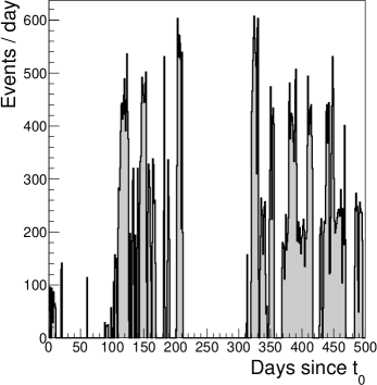
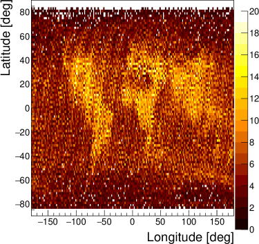
Figure 1: Distribution of the triggered events. Left panel: the time distribution from the first day of acquisition. Right panel: the geographical distribution of the triggers.

Most of the triggers can be grouped in sequences of about 2000 s (33 minutes) from the first to the last (see Fig. 2, left). As a matter of fact, 2000 s is the time that the satellite takes to cross the night side of the Earth and therefore such sequences can be associated to a single orbit of the satellite. The number of triggers per orbit is shown in the right panel of Fig. 2.

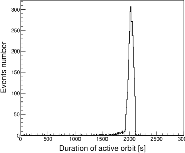
Figure 2: Left side: duration of the night time (or active time) of acquisition orbits. Right side: number of triggers per orbit.

As we have already mentioned above, TUS had a dead time from 52 to 60 seconds after each trigger, depending on the mission period, and therefore no orbits with more than $\sim 40$ triggers could be generally observed. An estimate of the active time can be therefore given for each orbit, under the assumption that the detector has always been in acquisition. Orbits with a high number of triggers have a very high fraction of dead time while, on the other hand, orbits with few triggers have a higher active time. This way, 3118 orbits with a total acquisition time of 73 full days were identified. A total active time of 31 days is obtained as soon as the dead time is taken into account. This amounts to $\sim 42\%$ of the total acquisition time. Such an estimate is based only on the identified orbits and could be potentially an underestimate of the real acquisition time.

Thanks to the knowledge of the satellite trajectory, it was possible to estimate with a $\sim 1$ second resolution the status of the detector for each position on the Earth map. The geographical distribution of active time fraction $\psi(\varphi,\lambda)=t_{\mathrm{act}}(\varphi,\lambda)/t_{\mathrm{tr}}(\varphi,\lambda)$ is shown in Fig. 3. In this formula, $t_{\mathrm{act}}$ is the amount of active time, $t_{\mathrm{tr}}$ is the total time integrated in a specific location of the Earth, $\varphi$ is the latitude and $\lambda$ is the longitude. It can be clearly seen that the presence of a higher trigger rate implies a higher dead time. As a consequence of that, populated areas or stormy regions are basically not contributing to the cumulated exposure. Aurora ovals are also clearly visible as non-active areas in the polar regions. On the other hand, oceans are very quiet areas, where cosmic ray studies would be favoured.

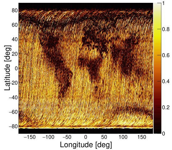
Figure 3: Ratio of active time over the total amount of transit time as a function of geographical location.

Positions of the Sun and the Moon were calculated based on data from the Japanese Coast Guard [5, 6]. All triggers could be therefore classified depending on the Moon illumination. The left panel of Figure 4 shows the distribution of the active time fraction $\psi(\varphi,\lambda)$. The fraction of data collected when the Moon was under horizon or under 20% phase (close to new moon) is shown in red. The whole data sample is shown in black. The presence of low or no-Moon illumination is verified in 21.2 full days of acquisition. The amount of active time in this condition amounts to 12.9 days, 60% of moonless acquisition time. It is clearly apparent that a cut on the Moon illumination, while decreasing the absolute amount of active time, would increase the data quality.

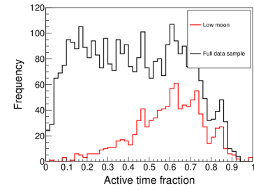
Figure 4: Left panel: active time distribution for each acquisition orbit. The full data set is shown in black. The distribution with low moon illumination is shown in red. Right panel: fraction of triggers with cloud top height under $h_{\mathrm{thr}}$.

The cloud condition for each trigger has been estimated based on MERRA data [7]. In Fig. 4 (right side) we plot the fraction of events where the cloud top height is lower than a threshold ($h_{\mathrm{thr}}$). It can be seen how most ($\sim 70\%$) of the triggers are in cloudy condition. It is therefore crucial to estimate the efficiency for cosmic ray detection in presence of clouds. Simulations will be used for this purpose and we will follow the approach described in [4].

The signal recorded for each triggered event can be used to estimate the rate of photoelectrons generated by the airglow emission. Such information is fundamental for the estimation of the performances of future space-based detectors since all trigger algorithms must cope with this emission. An accurate estimate of the airglow photon radiance requires detailed optics simulations which go beyond the scope of this publication and therefore we will only estimate the rate of photoelectrons per frame. Such information will be used in the simulations to estimate the energy dependence of the exposure. The conversion rate from ADC channels to photoelectrons is given by the following formula:

$$n_{0}=\alpha\frac{q_{e}}{C}\frac{RC}{\Delta t}G,$$ (1)

where $G$ is the gain of the channel, $C$ and $R$ are the capacitance and resistance in the anode RC chain of each PMT, $\Delta t$ is the time frame of TUS and $q_{e}$ is the charge of the electron. The calculation is performed only for the cases where the high voltage status flag was set to 255 ADC channels, or in other terms, where the high voltage setting was maximum. In such cases the measured gain values are reliable and Eq. (1) can be therefore used. The distribution of the background illumination obtained with the TUS data is shown in Figure 5.

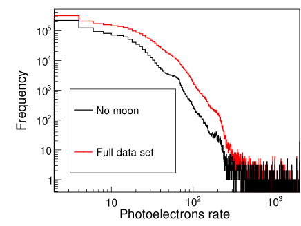
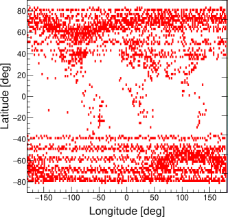
Figure 5: Left panel: estimated average photoelectron rate per pixel and time frame from airglow. Right panel: distribution of high background rate frames ($N_{\mathrm{ph}}>80$).

As it can be seen, the rate of the background illumination varies from 1 to over 100 photoelectrons per frame with some less common cases up to several thousand photoelectrons. The right panel of Figure 5 shows the geographical location of events where a rate higher than 80 photoelectrons per frame was detected. It is apparent that such extremely high rates were found in the Aurora ovals or above very densely populated areas. Several linear structures can be observed in the Southern hemisphere. They appeared to be due to the transition from nocturnal segments of orbits to regions where the satellite started to receive light from the Sun. Such data are collected during the Southern hemisphere summer in a sequence of acquisition sessions separated by few weeks. The shift from a dark region to a bright one causes the generation of triggers in a very limited space as it can be seen in the figure. The detector is then switched to low gain mode once the satellite enters in the full day light and all the following triggers are not taken into account anymore. All such high rate conditions can be identified as extreme cases and do not reduce the exposure in a significant way.

3 The TUS trigger performance

An estimate of the trigger performance is obtained through Monte Carlo simulations. Two thousand extensive air showers were injected in an area $A_{\mathrm{simu}}$ larger than the field of view ($\pm 150$ km) to avoid border effects. Showers were simulated with zenith angles from $0^{\circ}$ to $90^{\circ}$ and the azimuth from 0 to 360^∘. The TUS trigger logic was implemented in the ESAF simulation software [8] and used for this estimation. Several trigger thresholds used in the mission were tested with an airglow rate of $\sim 18$ photoelectrons per frame. The estimate of the trigger performance depends on a number of factors, among them the sensitivity of the photodetector, the level of the background illumination and software parameters of the trigger. During an incident described in [3], 20% of the PMTs were destroyed and sensitivities of the remaining PMTs changed in comparison with pre-flight measurements. A number of attempts of in-flight calibration have been performed but none of them is fully reliable yet. This introduces a large factor of uncertainty in estimates of the trigger threshold that can be wrong by a large amount. As a result of our preliminary estimation, we obtain a trigger threshold $\gtrsim 400$ EeV. Moreover, the TUS trigger algorithm is more efficient for horizontal showers leading to a higher fraction of high zenith angle events. The majority of the events could indeed trigger only above $40^{\circ}\text{--}50^{\circ}$. This is a consequence of the persistency condition of the trigger that rejects all events lasting for a short time.

A set of simulations has been performed to estimate the efficiency of the trigger in cloudy conditions. Thousand extensive air showers at fixed energy have been simulated for each cloud top height condition the same way as for clear sky. Table 1 presents the fraction of triggers with clouds below a specific altitude (as shown in the right panel of Figure 4 and indicated as $\eta(h<h_{\mathrm{thr}})$). The second row of Table 1 shows the ratio of the efficiency $\epsilon_{\mathrm{cloud}}$ obtained in cloudy conditions to the one obtained in clear sky ($\epsilon_{\mathrm{CS}}$).

	Clear sky	1 km	2 km	4 km	6 km	8 km	10 km	12 km	14 km
$\eta(h<h_{\mathrm{thr}})$	28$\%$	29$\%$	38$\%$	56$\%$	64$\%$	72$\%$	80$\%$	93$\%$	99.8$\%$
$\epsilon_{\mathrm{cloud}}$/ $\epsilon_{\mathrm{CS}}$	100$\%$	100$\%$	83$\%$	53$\%$	40$\%$	16$\%$	6$\%$	6$\%$	0$\%$

Table 1: Reduction of the trigger efficiency due to the presence of clouds with respect to clear sky at $2\times 10^{21}$ eV.

A higher cloud top height will cause a significant reduction of the triggered events given the reduction of the amount of light reaching the detector. An estimate of the overall reduction of the exposure in the whole flight can be given by an average of the trigger efficiency weighted by the fraction of triggers in each condition. Given the cloud conditions in the field of view at the time of the flight, an exposure of 57% of what is expected for the clear sky case has been estimated.

Airglow rate [ph / frame]	5	18	30	50	100
NTrigg./ NTrigg.,5	100$\%$	60$\%$	56$\%$	18$\%$	0$\%$

Table 2: Triggers fraction at $2\times 10^{21}$ eV with respect to the 5 photoelectrons / frame case.

The efficiency of the trigger was also estimated for different airglow rates. We tested 5, 18, 30, 50 and 100 photoelectrons / frame and estimated the number of triggers in each condition for a fixed energy. The lower rates are characterized by a higher efficiency. By assuming the rate at 5 photoelectrons / frame (N_Trigg.,5) to be 100%, we could estimate the change in the trigger rate shown in Tab. 2. As expected, we found a strong dependence of the efficiency on the airglow rate. For space-based observatories it will be therefore crucial to estimate the brightness of the field of view and the performances of the trigger in different illumination conditions.

4 Conclusions

Thanks to the analysis of the time distributions of the TUS triggers it was possible to identify a minimum of 3118 complete orbits of data acquisition. This has to be considered as a preliminary estimation given that particularly quiet orbits may not be counted at all in this analysis. By considering the number of triggers occurring in such orbits and the dead time occurring after each trigger, we identified 31 days of full time acquisition. The exposure is mainly concentrated on the oceans, deserts and in Antarctica while populated or stormy areas do not contribute to the total exposure given the very long dead time of TUS. A smaller dead time in future detectors will certainly reduce the severity of this loss of exposure. Moon-free data are characterized by a higher active time fraction. The estimation of the count rate from airglow gives a variable rate from a few photoelectrons per frame up to over 100. The most luminous parts of the Earth are the ones associated to the Aurora ovals, densely populated areas and to regions close to the terminator. The trigger performances must be still studied in detail but preliminary indications point to a trigger threshold $\gtrsim 400$ EeV. The presence of clouds reduces the exposure in this range by $\sim 40\%$. As expected, a strong dependence of the trigger performances on the field of view luminosity is found. The design of future missions must take carefully into account the variability of the field of view scenario and the trigger performances for various sky conditions. Under the above mentioned assumptions, the purely geometrical exposure of the TUS mission ($\mathscr{E}$), without clouds and for very high event luminosity, can be estimated as $\mathscr{E}=A_{\mathrm{FOV}}\times\Omega\times t$. The geometrical exposure amounts therefore to $\sim 1550~{}\mathrm{km}^{2}~{}\text{sr~{}yr}$.

5 Acknowledgements

The Russian group is supported by the State Space Corporation ROSCOSMOS and the Interdisciplinary Scientific and Educational School of Lomonosov Moscow University “Fundamental and Applied Space Research.” The Italian group acknowledges financial contribution from the agreement ASI-INAF n.2017-14-H.O.

Full Authors List: JEM-EUSO Collaboration

G. Abdellaoui^ah, S. Abe^fq, J.H. Adams Jr.^pd, D. Allard^cb, G. Alonso^md, L. Anchordoqui^pe, A. Anzalone^eh,ed, E. Arnone^ek,el, K. Asano^fe, R. Attallah^ac, H. Attoui^aa, M. Ave Pernas^mc, M. Bagheri^ph, J. Baláz^la, M. Bakiri^aa, D. Barghini^el,ek, S. Bartocci^ei,ej, M. Battisti^ek,el, J. Bayer^dd, B. Beldjilali^ah, T. Belenguer^mb, N. Belkhalfa^aa, R. Bellotti^ea,eb, A.A. Belov^kb, K. Benmessai^aa, M. Bertaina^ek,el, P.F. Bertone^pf, P.L. Biermann^db, F. Bisconti^el,ek, C. Blaksley^ft, N. Blanc^oa, S. Blin-Bondil^ca,cb, P. Bobik^la, M. Bogomilov^ba, K. Bolmgren^na, E. Bozzo^ob, S. Briz^pb, A. Bruno^eh,ed, K.S. Caballero^hd, F. Cafagna^ea, G. Cambié^ei,ej, D. Campana^ef, J-N. Capdevielle^cb, F. Capel^de, A. Caramete^ja, L. Caramete^ja, P. Carlson^na, R. Caruso^ec,ed, M. Casolino^ft,ei, C. Cassardo^ek,el, A. Castellina^ek,em, O. Catalano^eh,ed, A. Cellino^ek,em, K. Černý^bb, M. Chikawa^fc, G. Chiritoi^ja, M.J. Christl^pf, R. Colalillo^ef,eg, L. Conti^en,ei, G. Cotto^ek,el, H.J. Crawford^pa, R. Cremonini^el, A. Creusot^cb, A. de Castro Gónzalez^pb, C. de la Taille^ca, L. del Peral^mc, A. Diaz Damian^cc, R. Diesing^pb, P. Dinaucourt^ca, A. Djakonow^ia, T. Djemil^ac, A. Ebersoldt^db, T. Ebisuzaki^ft, J. Eser^pb, F. Fenu^ek,el, S. Fernández-González^ma, S. Ferrarese^ek,el, G. Filippatos^pc, W.I. Finch^pc C. Fornaro^en,ei, M. Fouka^ab, A. Franceschi^ee, S. Franchini^md, C. Fuglesang^na, T. Fujii^fg, M. Fukushima^fe, P. Galeotti^ek,el, E. García-Ortega^ma, D. Gardiol^ek,em, G.K. Garipov^kb, E. Gascón^ma, E. Gazda^ph, J. Genci^lb, A. Golzio^ek,el, C. González Alvarado^mb, P. Gorodetzky^ft, A. Green^pc, F. Guarino^ef,eg, C. Guépin^pl, A. Guzmán^dd, Y. Hachisu^ft, A. Haungs^db, J. Hernández Carretero^mc, L. Hulett^pc, D. Ikeda^fe, N. Inoue^fn, S. Inoue^ft, F. Isgrò^ef,eg, Y. Itow^fk, T. Jammer^dc, S. Jeong^gb, E. Joven^me, E.G. Judd^pa, J. Jochum^dc, F. Kajino^ff, T. Kajino^fi, S. Kalli^af, I. Kaneko^ft, Y. Karadzhov^ba, M. Kasztelan^ia, K. Katahira^ft, K. Kawai^ft, Y. Kawasaki^ft, A. Kedadra^aa, H. Khales^aa, B.A. Khrenov^kb, Jeong-Sook Kim^ga, Soon-Wook Kim^ga, M. Kleifges^db, P.A. Klimov^kb, D. Kolev^ba, I. Kreykenbohm^da, J.F. Krizmanic^pf,pk, K. Królik^ia, V. Kungel^pc, Y. Kurihara^fs, A. Kusenko^fr,pe, E. Kuznetsov^pd, H. Lahmar^aa, F. Lakhdari^ag, J. Licandro^me, L. López Campano^ma, F. López Martínez^pb, S. Mackovjak^la, M. Mahdi^aa, D. Mandát^bc, M. Manfrin^ek,el, L. Marcelli^ei, J.L. Marcos^ma, W. Marszał^ia, Y. Martín^me, O. Martinez^hc, K. Mase^fa, R. Matev^ba, J.N. Matthews^pg, N. Mebarki^ad, G. Medina-Tanco^ha, A. Menshikov^db, A. Merino^ma, M. Mese^ef,eg, J. Meseguer^md, S.S. Meyer^pb, J. Mimouni^ad, H. Miyamoto^ek,el, Y. Mizumoto^fi, A. Monaco^ea,eb, J.A. Morales de los Ríos^mc, M. Mastafa^pd, S. Nagataki^ft, S. Naitamor^ab, T. Napolitano^ee, J. M. Nachtman^pi A. Neronov^ob,cb, K. Nomoto^fr, T. Nonaka^fe, T. Ogawa^ft, S. Ogio^fl, H. Ohmori^ft, A.V. Olinto^pb, Y. Onel^pi G. Osteria^ef, A.N. Otte^ph, A. Pagliaro^eh,ed, W. Painter^db, M.I. Panasyuk^kb, B. Panico^ef, E. Parizot^cb, I.H. Park^gb, B. Pastircak^la, T. Paul^pe, M. Pech^bb, I. Pérez-Grande^md, F. Perfetto^ef, T. Peter^oc, P. Picozza^ei,ej,ft, S. Pindado^md, L.W. Piotrowski^ib, S. Piraino^dd, Z. Plebaniak^ek,el,ia, A. Pollini^oa, E.M. Popescu^ja, R. Prevete^ef,eg, G. Prévôt^cb, H. Prieto^mc, M. Przybylak^ia, G. Puehlhofer^dd, M. Putis^la, P. Reardon^pd, M.H.. Reno^pi, M. Reyes^me, M. Ricci^ee, M.D. Rodríguez Frías^mc, O.F. Romero Matamala^ph, F. Ronga^ee, M.D. Sabau^mb, G. Saccá^ec,ed, G. Sáez Cano^mc, H. Sagawa^fe, Z. Sahnoune^ab, A. Saito^fg, N. Sakaki^ft, H. Salazar^hc, J.C. Sanchez Balanzar^ha, J.L. Sánchez^ma, A. Santangelo^dd, A. Sanz-Andrés^md, M. Sanz Palomino^mb, O.A. Saprykin^kc, F. Sarazin^pc, M. Sato^fo, A. Scagliola^ea,eb, T. Schanz^dd, H. Schieler^db, P. Schovánek^bc, V. Scotti^ef,eg, M. Serra^me, S.A. Sharakin^kb, H.M. Shimizu^fj, K. Shinozaki^ia, J.F. Soriano^pe, A. Sotgiu^ei,ej, I. Stan^ja, I. Strharský^la, N. Sugiyama^fj, D. Supanitsky^ha, M. Suzuki^fm, J. Szabelski^ia, N. Tajima^ft, T. Tajima^ft, Y. Takahashi^fo, M. Takeda^fe, Y. Takizawa^ft, M.C. Talai^ac, Y. Tameda^fp, C. Tenzer^dd, S.B. Thomas^pg, O. Tibolla^he, L.G. Tkachev^ka, T. Tomida^fh, N. Tone^ft, S. Toscano^ob, M. Traïche^aa, Y. Tsunesada^fl, K. Tsuno^ft, S. Turriziani^ft, Y. Uchihori^fb, O. Vaduvescu^me, J.F. Valdés-Galicia^ha, P. Vallania^ek,em, L. Valore^ef,eg, G. Vankova-Kirilova^ba, T. M. Venters^pj, C. Vigorito^ek,el, L. Villaseñor^hb, B. Vlcek^mc, P. von Ballmoos^cc, M. Vrabel^lb, S. Wada^ft, J. Watanabe^fi, J. Watts Jr.^pd, R. Weigand Muñoz^ma, A. Weindl^db, L. Wiencke^pc, M. Wille^da, J. Wilms^da, D. Winn^pm T. Yamamoto^ff, J. Yang^gb, H. Yano^fm, I.V. Yashin^kb, D. Yonetoku^fd, S. Yoshida^fa, R. Young^pf, I.S Zgura^ja, M.Yu. Zotov^kb, A. Zuccaro Marchi^ft

^aa Centre for Development of Advanced Technologies (CDTA), Algiers, Algeria
^ab Dep. Astronomy, Centre Res. Astronomy, Astrophysics and Geophysics (CRAAG), Algiers, Algeria
^ac LPR at Dept. of Physics, Faculty of Sciences, University Badji Mokhtar, Annaba, Algeria
^ad Lab. of Math. and Sub-Atomic Phys. (LPMPS), Univ. Constantine I, Constantine, Algeria
^af Department of Physics, Faculty of Sciences, University of M’sila, M’sila, Algeria
^ag Research Unit on Optics and Photonics, UROP-CDTA, Sétif, Algeria
^ah Telecom Lab., Faculty of Technology, University Abou Bekr Belkaid, Tlemcen, Algeria
^ba St. Kliment Ohridski University of Sofia, Bulgaria
^bb Joint Laboratory of Optics, Faculty of Science, Palacký University, Olomouc, Czech Republic
^bc Institute of Physics of the Czech Academy of Sciences, Prague, Czech Republic
^ca Omega, Ecole Polytechnique, CNRS/IN2P3, Palaiseau, France
^cb Université de Paris, CNRS, AstroParticule et Cosmologie, F-75013 Paris, France
^cc IRAP, Université de Toulouse, CNRS, Toulouse, France
^da ECAP, University of Erlangen-Nuremberg, Germany
^db Karlsruhe Institute of Technology (KIT), Germany
^dc Experimental Physics Institute, Kepler Center, University of Tübingen, Germany
^dd Institute for Astronomy and Astrophysics, Kepler Center, University of Tübingen, Germany
^de Technical University of Munich, Munich, Germany
^ea Istituto Nazionale di Fisica Nucleare - Sezione di Bari, Italy
^eb Universita’ degli Studi di Bari Aldo Moro and INFN - Sezione di Bari, Italy
^ec Dipartimento di Fisica e Astronomia "Ettore Majorana", Universita’ di Catania, Italy
^ed Istituto Nazionale di Fisica Nucleare - Sezione di Catania, Italy
^ee Istituto Nazionale di Fisica Nucleare - Laboratori Nazionali di Frascati, Italy
^ef Istituto Nazionale di Fisica Nucleare - Sezione di Napoli, Italy
^eg Universita’ di Napoli Federico II - Dipartimento di Fisica "Ettore Pancini", Italy
^eh INAF - Istituto di Astrofisica Spaziale e Fisica Cosmica di Palermo, Italy
^ei Istituto Nazionale di Fisica Nucleare - Sezione di Roma Tor Vergata, Italy
^ej Universita’ di Roma Tor Vergata - Dipartimento di Fisica, Roma, Italy
^ek Istituto Nazionale di Fisica Nucleare - Sezione di Torino, Italy
^el Dipartimento di Fisica, Universita’ di Torino, Italy
^em Osservatorio Astrofisico di Torino, Istituto Nazionale di Astrofisica, Italy
^en Uninettuno University, Rome, Italy
^fa Chiba University, Chiba, Japan
^fb National Institutes for Quantum and Radiological Science and Technology (QST), Chiba, Japan
^fc Kindai University, Higashi-Osaka, Japan
^fd Kanazawa University, Kanazawa, Japan
^fe Institute for Cosmic Ray Research, University of Tokyo, Kashiwa, Japan
^ff Konan University, Kobe, Japan
^fg Kyoto University, Kyoto, Japan
^fh Shinshu University, Nagano, Japan
^fi National Astronomical Observatory, Mitaka, Japan
^fj Nagoya University, Nagoya, Japan
^fk Institute for Space-Earth Environmental Research, Nagoya University, Nagoya, Japan
^fl Graduate School of Science, Osaka City University, Japan
^fm Institute of Space and Astronautical Science/JAXA, Sagamihara, Japan
^fn Saitama University, Saitama, Japan
^fo Hokkaido University, Sapporo, Japan
^fp Osaka Electro-Communication University, Neyagawa, Japan
^fq Nihon University Chiyoda, Tokyo, Japan
^fr University of Tokyo, Tokyo, Japan
^fs High Energy Accelerator Research Organization (KEK), Tsukuba, Japan
^ft RIKEN, Wako, Japan
^ga Korea Astronomy and Space Science Institute (KASI), Daejeon, Republic of Korea
^gb Sungkyunkwan University, Seoul, Republic of Korea
^ha Universidad Nacional Autónoma de México (UNAM), Mexico
^hb Universidad Michoacana de San Nicolas de Hidalgo (UMSNH), Morelia, Mexico
^hc Benemérita Universidad Autónoma de Puebla (BUAP), Mexico
^hd Universidad Autónoma de Chiapas (UNACH), Chiapas, Mexico
^he Centro Mesoamericano de Física Teórica (MCTP), Mexico
^ia National Centre for Nuclear Research, Lodz, Poland
^ib Faculty of Physics, University of Warsaw, Poland
^ja Institute of Space Science ISS, Magurele, Romania
^ka Joint Institute for Nuclear Research, Dubna, Russia
^kb Skobeltsyn Institute of Nuclear Physics, Lomonosov Moscow State University, Russia
^kc Space Regatta Consortium, Korolev, Russia
^la Institute of Experimental Physics, Kosice, Slovakia
^lb Technical University Kosice (TUKE), Kosice, Slovakia
^ma Universidad de León (ULE), León, Spain
^mb Instituto Nacional de Técnica Aeroespacial (INTA), Madrid, Spain
^mc Universidad de Alcalá (UAH), Madrid, Spain
^md Universidad Politécnia de madrid (UPM), Madrid, Spain
^me Instituto de Astrofísica de Canarias (IAC), Tenerife, Spain
^na KTH Royal Institute of Technology, Stockholm, Sweden
^oa Swiss Center for Electronics and Microtechnology (CSEM), Neuchâtel, Switzerland
^ob ISDC Data Centre for Astrophysics, Versoix, Switzerland
^oc Institute for Atmospheric and Climate Science, ETH Zürich, Switzerland
^pa Space Science Laboratory, University of California, Berkeley, CA, USA
^pb University of Chicago, IL, USA
^pc Colorado School of Mines, Golden, CO, USA
^pd University of Alabama in Huntsville, Huntsville, AL; USA
^pe Lehman College, City University of New York (CUNY), NY, USA
^pf NASA Marshall Space Flight Center, Huntsville, AL, USA
^pg University of Utah, Salt Lake City, UT, USA
^ph Georgia Institute of Technology, USA
^pi University of Iowa, Iowa City, IA, USA
^pj NASA Goddard Space Flight Center, Greenbelt, MD, USA
^pk Center for Space Science & Technology, University of Maryland, Baltimore County, Baltimore, MD, USA
^pl Department of Astronomy, University of Maryland, College Park, MD, USA
^pm Fairfield University, Fairfield, CT, USA

References

- [1] P. A. Klimov et al. “The TUS detector of extreme energy cosmic rays on board the Lomonosov satellite” Space Science Reviews, 212:1687–1703, 2017, arXiv:1706.04976.
- [2] B. A. Khrenov et al. First results from the TUS orbital detector in the extensive air shower mode. Journal of Cosmology and Astroparticle Physics, 9:006, 2017, arXiv:1704.07704.
- [3] B. A. Khrenov et al. An extensive-air-shower-like event registered with the TUS orbital detector. Journal of Cosmology and Astroparticle Physics, 2020(3):033, arXiv:1907.06028.
- [4] The JEM–EUSO collaboration, "An evaluation of the exposure in nadir observation of the JEM–EUSO mission", Astrop. Phys. 44, 76-90 (2013)
- [5] https://www1.kaiho.mlit.go.jp/KOHO/syoshi/furoku/na16-data.pdf
- [6] https://www1.kaiho.mlit.go.jp/KOHO/syoshi/furoku/na16-rei.pdf
- [7] https://gmao.gsfc.nasa.gov/reanalysis/MERRA-2/
- [8] Berat et al., "ESAF: Full Simulation of Space–Based Extensive Air Showers Detectors", Astrop. Phys. Vol. 33, 4, P. 221–247 (2010)