Efficient Estimation of State-Space Mixed-Frequency VARs: A Precision-Based Approach

Abstract

State-space mixed-frequency vector autoregressions are now widely used for nowcasting. Despite their popularity, estimating such models can be computationally intensive, especially for large systems with stochastic volatility. To tackle the computational challenges, we propose two novel precision-based samplers to draw the missing observations of the low-frequency variables in these models, building on recent advances in the band and sparse matrix algorithms for state-space models. We show via a simulation study that the proposed methods are more numerically accurate and computationally efficient compared to standard Kalman-filter based methods. We demonstrate how the proposed method can be applied in two empirical macroeconomic applications: estimating the monthly output gap and studying the response of GDP to a monetary policy shock at the monthly frequency. Results from these two empirical applications highlight the importance of incorporating high-frequency indicators in macroeconomic models.

JEL classification: C11, C32, C51

Keywords: precision-based methods, band matrix, mixed-frequency, vector autogression, output gap, proxy VAR

1 Introduction

Mixed frequency vector autoregressions (MF-VARs) have become increasingly popular in empirical macroeconomics for forecasting and nowcasting. This popularity is due to them being more flexible for incorporating timely information over traditional VARs. A typical application is to nowcast real GDP, which is only available quarterly, using higher-frequency macroeconomic variables or financial indicators. There are two common approaches to handle mixed-frequency variables: the stacked approach and the state-space approach. The stacked MF-VAR approach of Ghysels (2016) estimates the mixed-frequency model at its lowest observed frequency; recent examples using this approach include McCracken, Owyang, and Sekhposyan (2020) and Koop, McIntyre, and Mitchell (2020). In contrast, the state-space approach of Schorfheide and Song (2015) treats the high-frequency observations of the low-frequency variables as missing values. These missing values are then estimated using standard Kalman filtering and smoothing algorithms. Recent applications of this approach include Brave, Butters, and Justiniano (2019) and Koop, McIntyre, Mitchell, and Poon (2020).

One key advantage of the state-space approach compared to the stacked approach is that it explicitly models all variables at the highest observed frequency. It allows the researcher to obtain the interpolated (historical) estimates of the low-frequency variables at a higher frequency. For example, using the state-space approach Schorfheide and Song (2015) provide monthly GDP estimates, which are required as inputs for a variety of applications. In addition, by modeling all variables at the highest observed frequency, the state-space approach delivers more timely nowcasts.

Nevertheless, the main drawback of the state-space approach is that its estimation tends to be computationally intensive. This large computational burden is mainly due to the simulation of the large number of latent states — i.e., missing observations of the low-frequency variables — using standard filtering and smoothing techniques. This computational burden becomes prohibitive when the dimension of the VAR becomes very large. This is a key obstacle in practice for using large state-space MF-VARs, despite the increasing popularity of large VARs in general since the seminal works by Bańbura, Giannone, and Reichlin (2010) and Koop (2013).

We overcome this computational challenge by proposing a novel precision-based approach for drawing the missing observations of the low-frequency variables in the state-space MF-VAR model. Precision-based sampling approaches for state-space models were first considered in Chan and Jeliazkov (2009) and McCausland, Miller, and Pelletier (2011), building upon earlier work by Rue (2001) on Gaussian Markov random fields. Due to their ease of implementation and computational efficiency, these precision-based samplers are increasingly used in a wide range of empirical applications. Recent examples include modeling trend inflation (Chan, Koop, and Potter, 2013, 2016; Chan, 2017; Hou, 2020), estimating the output gap (Grant and Chan, 2017a, b), macroeconomic forecasting (Cross and Poon, 2016; Cross, Hou, and Poon, 2019), modeling time-varying Phillips curve (Fu, 2020), and fitting various moving average models (Chan, 2013; Chan, Eisenstat, and Koop, 2016; Dimitrakopoulos and Kolossiatis, 2020; Zhang, Chan, and Cross, 2020) and dynamic factor models (Kaufmann and Schumacher, 2019; Beyeler and Kaufmann, 2021).

Our paper extends the precision-based sampling approach to state-space models with missing observations. More specifically, we derive the joint distribution of the missing observations (of the low-frequency variables) conditional on the high-frequency data and the model parameters. With the standard assumptions of Gaussian errors, we show that the conditional distribution of the missing observations is also Gaussian. A key feature of this conditional distribution is that its precision matrix is block-banded — i.e., it is sparse and its non-zero elements are arranged along a diagonal band. As such, the precision-based sampler of Chan and Jeliazkov (2009) can be applied to draw the missing observations. In particular, this novel approach allows us to draw all the missing observations in one step, and is especially efficient compared to standard filtering methods when the observation equation has a complex lag structure.

In addition, we allow the user to impose any linear constraints, both exactly and approximately, when sampling the missing observations. This feature is crucial in mixed-frequency applications as linear inter-temporal restrictions are typically imposed to map the high-frequency missing observations to match the observed values of the low-frequency variables. Our paper is related to the recent works by Eckert, Kronenberg, Mikosch, and Neuwirth (2020) and Hauber and Schumacher (2021), who also consider a precision-based sampling approach for settings with missing observations. However, they focus on dynamic factor models and the latter does not consider imposing linear constraints. As such, their methods are not directly applicable to state-space mixed-frequency VARs.

We conduct a series of simulated experiments to illustrate the numerical accuracy and computational speed of the proposed precision-based approach. In particular, we estimate the state-space MF-VARs using the proposed samplers and standard filtering methods under a variety of settings. We show that the proposed precision-based approach has two key advantages. First, it is more computationally efficient compared to standard Kalman-filter based methods and it scales well to high-dimensional settings. Second, it often delivers superior accuracy in estimating the missing observations of the low-frequency variables compared to standard filtering methods. As the number of low-frequency variables increases relative to high-frequency variables, the accuracy of standard filtering methods deteriorates significantly in estimating the missing observations due to numerical issues.

We demonstrate the proposed precision-based approach using two empirical macroeconomic applications. In the first application, we consider a large mixed-frequency Bayesian VAR with stochastic volatility and adaptive hierarchical priors to generate latent monthly estimates of real GDP and the corresponding output gap estimates using the framework of Morley and Wong (2020). More specifically, we estimate a 22-variable mixed-frequency Bayesian VAR consisting of 21 monthly macroeconomic and financial indicators and a quarterly real GDP measure using the proposed precision-based approach. We find that the monthly estimates of real GDP track all NBER recession dates well and give plausible values during the COVID-19 pandemic. Furthermore, the monthly output gap estimates, in specific periods, can differ from the Congressional Budget Office (CBO) quarterly output gap measure. A potential explanation for this difference could be the additional information extracted from the higher frequency monthly financial indicators. This highlights the importance of incorporating higher frequency indicators when estimating the output gap.

In the second empirical application, we extend the Bayesian Proxy VAR in Caldara and Herbst (2019) to a mixed-frequency setting. More specifically, we expand their VAR with only monthly variables to include a quarterly real GDP measure. We find that all the impulse responses of the monthly endogenous variables to a monetary policy shock, identified via a proxy variable, display precisely the same dynamics as presented in Caldara and Herbst (2019). However, the key difference is that the response of real GDP to a monetary policy shock appears to be more subdued compared to the response of industrial production. For example, the posterior median response of industrial production falls to a low of $-$0.5%, while the posterior median response of real GDP never falls below $-$0.2%. This result therefore suggests that the response of industrial production to a monetary policy shock might not be a good proxy for the response of the real economy. This again highlights the value of mixed-frequency VARs.

The remainder of the paper is organised as follows. Section 2 discusses the precision-based sampling approach for drawing the missing observations in a state-space MF-VAR model. Section 3 presents the results from a simulation study comparing the proposed mixed-frequency precision-based samplers against standard Kalman-filter based techniques. Section 4 illustrates how the proposed mixed-frequency precision-based approach can be applied to two popular empirical macroeconomic applications. Finally, Section 5 concludes.

2 Mixed-Frequency Precision-Based Samplers

This section introduces the proposed precision-based samplers for drawing the missing observations of the low-frequency variables within a state-space MF-VAR. More specifically, in the first subsection, we derive the conditional distribution of the missing observations given the observed data for the model and provide an efficient algorithm to draw from this conditional distribution. Next, in the second subsection, we show how the draws of the conditional distribution of the missing observations can be constrained to incorporate inter-temporal restrictions.

2.1 The Conditional Distribution of the Missing Observations

Following Schorfheide and Song (2015), we express the autoregression at the highest observed frequency. More specifically, let $\mathbf{y}_{t}^{o}$ denote the $n_{o}\times 1$ vector of high-frequency variables that are observed and let $\mathbf{y}_{t}^{u}$ represent the $n_{u}\times 1$ vector of low-frequency variables that are unobserved or only partially observed. A standard example frequently employed in the literature is as follows: $\mathbf{y}_{t}^{o}$ consists of $n_{o}$ monthly variables that are observed at every month $t$, whereas $\mathbf{y}_{t}^{u}$ consists of $n_{u}$ quarterly variables at monthly frequency that are only observed every 3 months (or the linear combination of the 3 monthly variables is observed).

Then, a mixed-frequency vector autoregression (MF-VAR) with $p$ lags for $\mathbf{y}_{t}=(\mathbf{y}_{t}^{o^{\prime}},\mathbf{y}_{t}^{u^{\prime}})^{\prime}$ of dimension $n=n_{o}+n_{u}$ can be written as:

$$\mathbf{y}_{t}=\mathbf{b}_{0}+\mathbf{B}_{1}\mathbf{y}_{t-1}+\mathbf{B}_{2}\mathbf{y}_{t-2}+\cdots+\mathbf{B}_{p}\mathbf{y}_{t-p}+\boldsymbol{\varepsilon}_{t},\quad\boldsymbol{\varepsilon}_{t}\sim\mathcal{N}(\mathbf{0},\boldsymbol{\Sigma}),$$ (1)

where $t=p+1,\ldots,T$, $\mathbf{b}_{0}$ is an $n\times 1$ vector of intercepts, $\mathbf{B}_{1},\ldots,\mathbf{B}_{p}$ are the $n\times n$ VAR coefficients and $\boldsymbol{\Sigma}$ is error covariance matrix. In what follows, the analysis is based on the joint distribution of $\mathbf{y}_{p+1},\ldots,\mathbf{y}_{T}$ conditional on the initial conditions $\mathbf{y}_{1},\ldots,\mathbf{y}_{p}$.

Below we derive the joint distribution of the unobserved (low-frequency) variables conditional on the observed (high-frequency) variables. Stacking $\mathbf{Y}=(\mathbf{y}_{1}^{\prime},\ldots,\mathbf{y}^{\prime}_{T})^{\prime}$, we can rewrite (1) as a standard linear regression in matrix form:

$$\mathbf{H}\mathbf{Y}=\mathbf{c}+\boldsymbol{\varepsilon},\quad\boldsymbol{\varepsilon}\sim\mathcal{N}(\mathbf{0},\boldsymbol{\Xi}),$$ (2)

where $\mathbf{c}=\mathbf{1}_{T-p}\otimes\mathbf{b}_{0}$, $\boldsymbol{\varepsilon}=(\boldsymbol{\varepsilon}_{p+1}^{\prime},\ldots,\boldsymbol{\varepsilon}_{T}^{\prime})^{\prime}$, $\boldsymbol{\Xi}=\mathbf{I}_{T-p}\otimes\boldsymbol{\Sigma}$, and

$$\mathbf{H}= \left[\begin{array}[]{cccccccc}-\mathbf{B}_{p}&\cdots&-\mathbf{B}_{1}&\mathbf{I}_{n}&\mathbf{O}_{n}&\cdots&\cdots&\mathbf{O}_{n}\\ \mathbf{O}_{n}&-\mathbf{B}_{p}&\cdots&-\mathbf{B}_{1}&\mathbf{I}_{n}&\mathbf{O}_{n}&\cdots&\mathbf{O}_{n}\\ \vdots&\ddots&\ddots&&\ddots&\ddots&\ddots&\vdots\\ \mathbf{O}_{n}&\cdots&\mathbf{O}_{n}&-\mathbf{B}_{p}&\cdots&-\mathbf{B}_{1}&\mathbf{I}_{n}&\mathbf{O}_{n}\\ \mathbf{O}_{n}&\cdots&\cdots&\mathbb{\mathbf{O}}_{n}&-\mathbf{B}_{p}&\cdots&-\mathbf{B}_{1}&\mathbf{I}_{n}\end{array}\right].$$

In the above expression, $\mathbf{1}_{T-p}$ is a $(T-p)\times 1$ column vector of ones, $\mathbf{I}_{T-p}$ is the identity matrix of dimension $T-p$, and $\mathbf{O}_{n}$ is the $n\times n$ zero matrix. Note that $\mathbf{H}$ is of dimension $Tn\times(T-p)n$ and is banded — i.e., it is a sparse matrix whose non-zero elements are arranged along a diagonal band.

Furthermore, one can write $\mathbf{Y}$ as a linear combination of the observed (high-frequency) and unobserved (low-frequency) variables as:

$$\mathbf{Y}=\mathbf{M}_{o}\mathbf{Y}^{o}+\mathbf{M}_{u}\mathbf{Y}^{u},$$ (3)

where $\mathbf{Y}^{o}=(\mathbf{y}_{1}^{o^{\prime}},\ldots,\mathbf{y}_{T}^{o^{\prime}})^{\prime}$ is a $Tn_{o}\times 1$ vector of the observed variables, $\mathbf{Y}^{u}=(\mathbf{y}_{1}^{u^{\prime}},\ldots,\mathbf{y}_{T^{\prime}}^{u})^{\prime}$ is a $Tn_{u}\times 1$ vector of the unobserved variables, and $\mathbf{M}_{o}$ and $\mathbf{M}_{u}$ are, respectively, $Tn\times Tn_{o}$ and $Tn\times Tn_{u}$ selection matrices that have full column rank. Substituting (3) into (2), we have

$$\mathbf{H}(\mathbf{M}_{o}\mathbf{Y}^{o}+\mathbf{M}_{u}\mathbf{Y}^{u})=\mathbf{c}+\boldsymbol{\varepsilon},\quad\boldsymbol{\varepsilon}\sim\mathcal{N}(\mathbf{0},\boldsymbol{\Xi}).$$ (4)

Now, conditional on $\mathbf{Y}^{o}$ (and the model parameters $\mathbf{B}=(\mathbf{b}_{0},\mathbf{B}_{1},\ldots,\mathbf{B}_{p})^{\prime}$ and $\boldsymbol{\Sigma}$), the joint density of $\mathbf{Y}^{u}$ can be expressed as

$$p(\mathbf{Y}^{u}\,|\,\mathbf{Y}^{o},\mathbf{B},\boldsymbol{\Sigma})\propto \exp\left\{-\frac{1}{2}\left(\mathbf{H}(\mathbf{M}_{o}\mathbf{Y}^{o}+\mathbf{M}_{u}\mathbf{Y}^{u})-\mathbf{c}\right)^{\prime}\boldsymbol{\Xi}^{-1}\left(\mathbf{H}(\mathbf{M}_{o}\mathbf{Y}^{o}+\mathbf{M}_{u}\mathbf{Y}^{u})-\mathbf{c}\right)\right\}$$

$$\propto \exp\left\{-\frac{1}{2}\left[\mathbf{Y}^{u^{\prime}}\mathbf{M}_{u}^{\prime}\mathbf{H}^{\prime}\boldsymbol{\Xi}^{-1}\mathbf{H}\mathbf{M}_{u}\mathbf{Y}^{u}-2\mathbf{Y}^{u^{\prime}}\mathbf{M}_{u}^{\prime}\mathbf{H}^{\prime}\boldsymbol{\Xi}^{-1}(\mathbf{c}-\mathbf{H}\mathbf{M}\mathbf{Y}^{o})\right]\right\}.$$

Let $\mathbf{K}_{\mathbf{Y}^{u}}=\mathbf{M}_{u}^{{}^{\prime}}\mathbf{H}^{\prime}\boldsymbol{\Xi}^{-1}\mathbf{H}\mathbf{M}_{u}$, which is a $Tn_{u}\times Tn_{u}$ non-singular matrix (as $\mathbf{H}\mathbf{M}_{u}$ has full column rank). Furthermore, let $\boldsymbol{\mu}_{\mathbf{Y}^{u}}=\mathbf{K}_{\mathbf{Y}^{u}}^{-1}\left(\mathbf{M}_{u}^{{}^{\prime}}\mathbf{H}^{\prime}\boldsymbol{\Xi}^{-1}(\mathbf{c}-\mathbf{H}\mathbf{M}_{o}\mathbf{Y}^{o})\right).$ Then, by completing the square in $\mathbf{Y}^{u}$, one can write the conditional density of $\mathbf{Y}^{u}$ as

$$p(\mathbf{Y}^{u}\,|\,\mathbf{Y}^{o},\mathbf{B},\boldsymbol{\Sigma})\propto \exp\left\{-\frac{1}{2}\left(\mathbf{Y}^{u^{\prime}}\mathbf{K}_{\mathbf{Y}^{u}}\mathbf{Y}^{u}-2\mathbf{Y}^{u^{\prime}}\mathbf{K}_{\mathbf{Y}^{u}}\boldsymbol{\mu}_{\mathbf{Y}^{u}}\right)\right\}$$

$$\propto \exp\left\{-\frac{1}{2}\left(\mathbf{Y}^{u}-\boldsymbol{\mu}_{\mathbf{Y}^{u}}\right)^{\prime}\mathbf{K}_{\mathbf{Y}^{u}}\left(\mathbf{Y}^{u}-\boldsymbol{\mu}_{\mathbf{Y}^{u}}\right)\right\}.$$

Thus, we have shown that the conditional distribution of the missing observations given the observed data is Gaussian:

$$(\mathbf{Y}^{u}\,|\,\mathbf{Y}^{o},\mathbf{B},\boldsymbol{\Sigma})\sim\mathcal{N}\left(\boldsymbol{\mu}_{\mathbf{Y}^{u}},\mathbf{K}_{\mathbf{Y}^{u}}^{-1}\right).$$ (5)

Since $\mathbf{H},\boldsymbol{\Xi}$ and $\mathbf{M}_{u}$ are all band matrices, so is the precision matrix $\mathbf{K}_{\mathbf{Y}^{u}}$. Therefore, we can use the precision-based sampler of Chan and Jeliazkov (2009) to draw $\mathbf{Y}^{u}$ efficiently. We also note that the conditional distribution derived in (5) has the same structure even when we allow for time-varying covariance matrices in the state-space MF-VAR model. The only minor change in the expression is that the block-diagonal matrix $\boldsymbol{\Xi}$ now depends on the time-varying covariance matrices $\boldsymbol{\Sigma}_{t},t=p+1,\ldots,T$.

2.2 Inter-Temporal Restrictions

So far the vector of missing observations $\mathbf{Y}^{u}$ is unrestricted. In practice, however, inter-temporal constraints on $\mathbf{Y}^{u}$ are often imposed to map the missing values to the observed values of the low-frequency variables. For example, a commonly employed inter-temporal constraint for log-differenced variables is the log-linear approximation of Mariano and Murasawa (2003, 2010). More specifically, suppose $y_{i,t}^{u}$ is the missing monthly value of the $i$-th variable at month $t$. Let $\widetilde{y}_{i,t}^{u}$ denote the corresponding observed quarterly value (note that $\widetilde{y}_{i,t}^{u}$ is only observed for every third month). Then, a standard log-linear approximation to an arithmetic average of the quarterly variable can be expressed as:

$$\widetilde{y}_{i,t}^{u}=\frac{1}{3}y_{i,t}^{u}+\frac{2}{3}y_{i,t-1}^{u}+y_{i,t-2}^{u}+\frac{2}{3}y_{i,t-3}^{u}+\frac{1}{3}y_{i,t-4}^{u}.$$ (6)

Stacking the inter-temporal constraints in (6) over time, we obtain

$$\widetilde{\mathbf{Y}}^{u}=\mathbf{M}_{a}\mathbf{Y}^{u},$$ (7)

where $\mathbf{M}_{a}$ is the $k\times Tn_{u}$ matrix specifying the $k$ linear restrictions in (6), and $\widetilde{\mathbf{Y}}^{u}$ contains the observed values of the low-frequency variables. As an example, for balanced monthly and quarterly variables, $k=Tn_{u}/3$.

Since for many commonly employed inter-temporal restrictions, the relationships between the missing and observed data are approximate rather than exact, we also consider a version with measurement or approximation errors:

$$\widetilde{\mathbf{Y}}^{u}=\mathbf{M}_{a}\mathbf{Y}^{u}+\mathbf{u},\quad\mathbf{u}\sim\mathcal{N}(\mathbf{0},\mathbf{O}),$$ (8)

where $\mathbf{O}$ is a fixed diagonal covariance matrix that encodes the magnitude of the measurement errors.

Next, we discuss how one can impose the hard and soft inter-temporal restrictions in (7) and (8), respectively. First, to incorporate the information encoded in the hard inter-temporal restrictions, we aim to sample $\mathbf{Y}^{u}$ from the Gaussian distribution in (5) subject to the linear constraint given in (7). An efficient way to do so is given in Algorithm 2.6 in Rue and Held (2005) and Algorithm 2 in Cong, Chen, and Zhou (2017). More specifically, we first draw $\mathbf{Z}$ from the unconstrained distribution as $\mathbf{Z}\sim\mathcal{N}\left(\boldsymbol{\mu}_{\mathbf{Y}^{u}},\mathbf{K}_{\mathbf{Y}^{u}}^{-1}\right)$. We then correct for the constraint by computing

$$\mathbf{Y}^{u}=\mathbf{Z}+\mathbf{K}_{\mathbf{Y}^{u}}^{-1}\mathbf{M}_{a}^{{}^{\prime}}(\mathbf{M}_{a}\mathbf{K}_{\mathbf{Y}^{u}}^{-1}\mathbf{M}_{a}^{{}^{\prime}})^{-1}(\widetilde{\mathbf{Y}}^{u}-\mathbf{M}_{a}\mathbf{Z}).$$

It can be shown that $\mathbf{Y}^{u}$ has the correct distribution, i.e., it follows the $\mathcal{N}\left(\boldsymbol{\mu}_{\mathbf{Y}^{u}},\mathbf{K}_{\mathbf{Y}^{u}}^{-1}\right)$ distribution satisfying the constraint $\widetilde{\mathbf{Y}}^{u}=\mathbf{M}_{a}\mathbf{Y}^{u}$. Algorithm 1 describes an efficient implementation in Rue and Held (2005) that avoids explicitly computing the inverse of $\mathbf{K}_{\mathbf{Y}^{u}}$ or $\mathbf{M}_{a}\mathbf{K}_{\mathbf{Y}^{u}}^{-1}\mathbf{M}_{a}^{{}^{\prime}}$. Using this implementation, the additional computational cost for correcting the constraint is relatively low for $k\ll Tn_{u}$. For large $k$, this algorithm would involve a few large, dense matrices, and the computations could be more intensive.

Algorithm 1 Sampling $(\mathbf{Y}^{u}\,|\,\widetilde{\mathbf{Y}}^{u}=\mathbf{M}_{a}\mathbf{Y}^{u})$ with hard inter-temporal restrictions, where $\mathbf{Y}^{u}\sim\mathcal{N}\left(\boldsymbol{\mu}_{\mathbf{Y}^{u}},\mathbf{K}_{\mathbf{Y}^{u}}^{-1}\right)$.

Given the parameters $\boldsymbol{\mu}_{\mathbf{Y}^{u}}$ and $\mathbf{K}_{\mathbf{Y}^{u}}$, complete the following steps.

1. Obtain the Cholesky factor $\mathbf{C}$ of $\mathbf{K}_{\mathbf{Y}^{u}}$ such that $\mathbf{K}_{\mathbf{Y}^{u}}=\mathbf{C}\mathbf{C}^{\prime}$

2. Solve $\mathbf{C}^{\prime}\mathbf{v}=\mathbf{x}$ for $\mathbf{v}$ by backward substitution, where $\mathbf{x}\sim\mathcal{N}(\mathbf{0},\mathbf{I}_{Tn_{u}})$

3. Compute $\mathbf{Z}=\boldsymbol{\mu}_{\mathbf{Y}^{u}}+\mathbf{v}$

4. Solve $\mathbf{C}\mathbf{C}^{\prime}\mathbf{V}=\mathbf{M}_{a}^{\prime}$ for $\mathbf{V}$ by forward and backward substitution

5. Solve $\mathbf{W}\mathbf{U}=\mathbf{V}^{\prime}$ for $\mathbf{U}$, where $\mathbf{W}=\mathbf{M}_{a}\mathbf{V}$

6. Return $\mathbf{Y}^{u}=\mathbf{Z}+\mathbf{U}^{\prime}(\widetilde{\mathbf{Y}}^{u}-\mathbf{M}_{a}\mathbf{Z})$

Next, to incorporate the soft inter-temporal restrictions, one can view (7) as a new measurement equation and the Gaussian distribution of $\mathbf{Y}^{u}$ in (5) as the “prior distribution”. Then, by standard linear regression results, we obtain

$$(\mathbf{Y}^{u}\,|\,\mathbf{Y}^{o},\widetilde{\mathbf{Y}}^{u},\mathbf{B},\boldsymbol{\Sigma})\sim\mathcal{N}\left(\overline{\boldsymbol{\mu}}_{\mathbf{Y}^{u}},\overline{\mathbf{K}}_{\mathbf{Y}^{u}}^{-1}\right),$$ (9)

where

$$\overline{\mathbf{K}}_{\mathbf{Y}^{u}}=\mathbf{M}_{a}^{\prime}\mathbf{O}^{-1}\mathbf{M}_{a}+\mathbf{K}_{\mathbf{Y}^{u}},\quad\overline{\boldsymbol{\mu}}_{\mathbf{Y}^{u}}=\overline{\mathbf{K}}_{\mathbf{Y}^{u}}^{-1}\left(\mathbf{M}_{a}^{\prime}\mathbf{O}^{-1}\widetilde{\mathbf{Y}}^{u}+\mathbf{K}_{\mathbf{Y}^{u}}\boldsymbol{\mu}_{\mathbf{Y}^{u}}\right).$$

Since the matrices $\mathbf{M}_{a},\mathbf{O}$ and $\mathbf{K}_{\mathbf{Y}^{u}}$ are all banded, so is $\overline{\mathbf{K}}_{\mathbf{Y}^{u}}$. Hence, the precision-based sampler of Chan and Jeliazkov (2009) can be directly applied to sample $\mathbf{Y}^{u}$ efficiently. Compared to Algorithm 1 for the hard inter-temporal constraints, sampling from (9) is much faster and scales well to high-dimensional settings. For approximate inter-temporal restrictions such as Mariano and Murasawa (2003, 2010), the latter sampler is naturally preferable. For other exact inter-temporal restrictions, empirically one can approximate these hard restrictions by setting the diagonal elements of $\mathbf{O}$ to be very small (e.g., $10^{-8}$). Therefore, we use the sampling scheme in (9) as the baseline.

3 A Simulation Study

We conduct a simulation study to assess the speed and accuracy of the proposed precision-based methods for drawing the latent missing observations of the low-frequency variables relative to Kalman-filter based methods. In what follows, all data-generating processes (DGPs) assume the following VAR structure with $p=4$ lags:

$$\mathbf{y}_{t}=\mathbf{b}_{0}+\mathbf{B}_{1}\mathbf{y}_{t-1}+\mathbf{B}_{2}\mathbf{y}_{t-2}+\mathbf{B}_{3}\mathbf{y}_{t-3}+\mathbf{B}_{4}\mathbf{y}_{t-4}+\boldsymbol{\varepsilon}_{t},\quad\boldsymbol{\varepsilon}_{t}\sim\mathcal{N}(\mathbf{0},\boldsymbol{\Sigma}),$$

where $\mathbf{y}_{t}=(\mathbf{y}_{t}^{o^{\prime}},\mathbf{y}_{t}^{u^{\prime}})$ is an $n\times 1$ vector of mixed-frequency data, $\mathbf{y}_{t}^{o}$ is the $n_{o}\times 1$ vector of the high-frequency variables and $\mathbf{y}_{t}^{u}$ is the $n_{u}\times 1$ vector of the low-frequency variables. We set $\mathbf{b}_{0}=0.01\times\mathbf{1}_{n}$, $\mathbf{B}_{1}=0.5\times\mathbf{I}_{n}$, $\mathbf{B}_{2}=0.05\times\mathbf{I}_{n}$, $\mathbf{B}_{3}=0.001\times\mathbf{I}_{n}$, $\mathbf{B}_{4}=0.0001\times\mathbf{I}_{n}$, and $\boldsymbol{\Sigma}=0.01\times\mathbf{I}_{n}$.

We consider DGPs of different dimensions with $T=500$: small ($n=5,n_{o}=4,n_{u}=~{}1)$, medium ($n=11,n_{o}=10,n_{u}=1)$ and large ($n=21,n_{o}=20,n_{u}=1)$. We also investigate settings with a larger number of unobserved variables ($n_{u}=5$). For each simulated dataset $r=1,\ldots,R$, we estimate the missing observations $\mathbf{y}_{t}^{u,r}$ using 3 methods: precision-based sampler with hard inter-temporal constraints in (7), precision-based sampler with soft constraints in (8), and the simulation smoother of Carter and Kohn (1994) as implemented in the code provided by Schorfheide and Song (2015). Lastly, for all VARs we assume the standard normal-inverse-Wishart prior with non-informative hyperparameters.

To assess the accuracy of the proposed methods, we compute the mean squared errors (MSEs) of the estimated missing observations against the actual simulated values. The MSEs of all methods are computed using $R=10$ simulations, and the results are displayed in Table 1. We also report the computation times, based on 20,000 MCMC draws with a burn-in period of 10,000 draws. Since the three methods aim to draw from the same distribution — namely, the conditional distribution of the missing observations given the observed data and model parameters — in principle they should give the same MSEs (modulo Monte Carlo errors). Indeed, they tend to give very similar MSEs when the ratio $n_{o}/n_{u}$ is sufficiently large. However, when $n_{u}$, the number of variables with missing observations, is large relative to $n_{o}$, the number of fully observed variables, the accuracy of the Kalman-filter based method appears to deteriorate significantly relative to the proposed methods, possibly due to numerical errors. In terms of runtime, it is clear that the proposed precision-based methods are more computationally efficient compared to the Kalman-filter based method across a range of settings.

Table 1: Mean squared errors of the estimated missing observations and computation times using three methods: the proposed precision-based method with hard inter-temporal constraints (Precision-hard), the precision-based method with soft inter-temporal constraints (Precision-soft) and the simulation smoother of Carter and Kohn (1994) implemented in Schorfheide and Song (2015) (KF).

		MSE			Computation time (minutes)
$n_{u}$	$n_{o}$	Precision-hard	Precision-soft	KF	Precision-hard	Precision-soft	KF
1	4	0.014	0.024	0.029	0.8	1	6
1	10	0.015	0.024	0.019	3	3	8
1	20	0.018	0.023	0.021	25	26	36
5	4	0.899	0.222	2.140	13	3	26
5	10	0.035	0.029	0.070	11	10	30
5	20	0.023	0.025	0.027	64	54	73

Table 1 reports the runtimes of full MCMC estimation. When the dimension of the VAR increases, the part of the posterior sampler that simulates the VAR coefficients dominates, and it gives the impression that the runtimes of the three methods converge. To better understand how the proposed methods perform across a wider range of settings, next we compare only the runtimes of sampling the missing observations.

First, Figure 1 reports the runtimes of sampling 10 draws of the missing observations using the three methods for a range of $n_{o}$ and $n_{u}$. It is clear that both precision-based methods compare favorably to the Kalman-filter based method, and both scale well to high dimensional settings. In addition, the variant with soft constrictions is especially efficient when there are a large number of variables with missing observations.

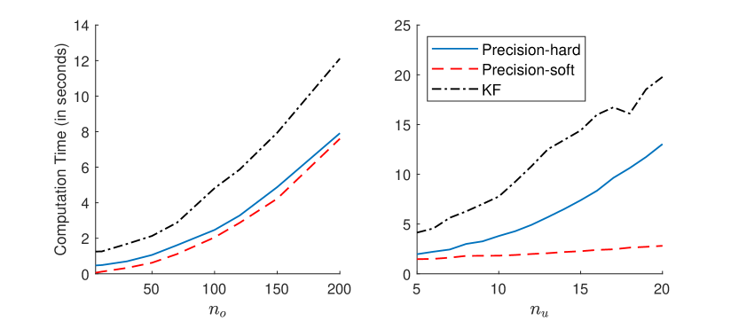
Figure 1: Computation times of obtaining 10 draws againist $n_{o}$ and $n_{u}$, the numbers of observed and partially unobserved variables, respectively, with $T=500$ and $p=4$. The three methods are: precision-based sampler with hard inter-temporal constraints (Precision-hard), precision-based sampler with soft constraints (Precision-soft) and the simulation smoother of Carter and Kohn (1994) implemented in Schorfheide and Song (2015) (KF).

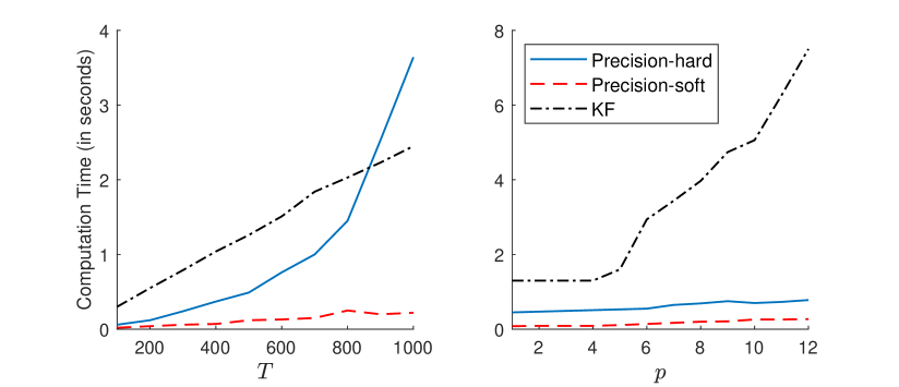
Figure 2: Computation times of obtaining 10 draws against $T$ and $p$, the numbers of time periods and lags, respectively, with $n_{u}=5$ and $n_{o}=10$. The three methods are: precision-based sampler with hard inter-temporal constraints (Precision-hard), precision-based sampler with soft constraints (Precision-soft) and the simulation smoother of Carter and Kohn (1994) implemented in Schorfheide and Song (2015) (KF).

Next, Figure 2 reports the runtimes of sampling ten draws of the missing observations for a range of sample sizes $T$ and lag lengths $p$. While both precision-based methods perform well, the version with soft constrictions does substantially better and scales well to very large $T$ and $p$. It is also worth mentioning that to apply the Kalman filter, and one needs to redefine the states so that the observation equation depends only on the current (redefined) state. When $p$ is large, the dimension of this new state vector is large. And that is the reason why the Kalman-filter based method becomes very computationally intensive when $p$ is large. In contrast, the computational costs of the precision-based methods remain low even for long lag lengths.

4 Empirical Applications

We demonstrate the proposed mixed-frequency precision-based samplers via two popular empirical macroeconomic applications. First, we show that the proposed samplers can be incorporated efficiently within a state-of-the-art large Bayesian VAR with stochastic volatility and global-local priors. Furthermore, we also show that we can derive monthly estimates of the US output gap using the framework of Morley and Wong (2020). In the second application, we extend the methodology in Caldara and Herbst (2019) by proposing a novel mixed-frequency Bayesian Proxy VAR estimated using the proposed samplers.

4.1 A State-Space Mixed-Frequency VAR with Stochastic Volatility and Global-Local Priors

Since the seminal works by Bańbura, Giannone, and Reichlin (2010) and Koop (2013), large Bayesian VARs have become increasingly popular in empirical macroeconomics. However, large Bayesian VARs tend to be over-parameterised, and a key way to overcome this problem is to implement shrinkage priors, such as the Minnesota prior (Doan, Litterman, and Sims, 1984; Litterman, 1986) and the more recent global-local priors (see Polson and Scott, 2010; Huber and Feldkircher, 2019; Cross, Hou, and Poon, 2019). Another popular feature researchers and practitioners incorporate within a large Bayesian VAR is stochastic volatility (SV). There are a large number of studies that document the importance of allowing for SV (or a time-varying covariance structure) when modelling macroeconomic data (see, e.g., Clark, 2011; Clark and Ravazzolo, 2015; Carriero, Clark, and Marcellino, 2019).

Recently, Chan (2021) introduced a class of Minnesota-type adaptive hierarchical priors for large Bayesian VARs with SV. In a nutshell, these new priors combine the advantages of both the Minnesota prior (e.g., rich prior beliefs such as cross-variable shrinkage) and global-local priors (e.g., heavy-tails and substantial mass around 0). These new priors are shown to provide superior forecasts compared to both the Minnesota prior and conventional global-local priors.

In this first application, we extend the large Bayesian VAR in Chan (2021) to a mixed-frequency state-space setting and estimate the model using the proposed precision-based samplers. We mostly follow the model assumptions specified in Chan (2021) and estimate a 22-variable mixed-frequency VAR with SV (denoted here as MF-BVAR-SV) with $p=4$ lags. The variables consist of 21 monthly macroeconomic indicators and a quarterly real GDP measure. This exercise is motivated by recent interest in more timely monthly estimates of real GDP (see, e.g., Brave, Butters, and Kelley, 2019). A more timely measure of GDP allows policymakers to react to economic shocks more rapidly. Therefore, our primary focus of this application is in generating the latent monthly estimates for real GDP and the corresponding output gap.

The complete list of the 22 variables and their transformations are presented in Table 3 in the appendix. The sample covers 1960M1-2021M3 (and 1960Q1-2021Q1), which includes the pandemic period. The 21 monthly macroeconomic indicators are selected so that they are broadly similar to the dataset considered in Morley and Wong (2020). The majority of the variables are log-differenced to ensure stationarity. In addition, we impose the standard inter-temporal constraint of Mariano and Murasawa (2003, 2010) on the quarterly real GDP

$$y_{t}^{GDP,Q}=\frac{1}{3}y_{t}^{GDP,m}+\frac{2}{3}y_{t-1}^{GDP,m}+y_{t-2}^{GDP,m}+\frac{2}{3}y_{t-3}^{GDP,m}+\frac{1}{3}y_{t-4}^{GDP,m},$$

where $y_{t}^{GDP,Q}$ and $y_{t}^{GDP,m}$ are the observed quarterly and latent monthly real GDP variables at time $t$, respectively.

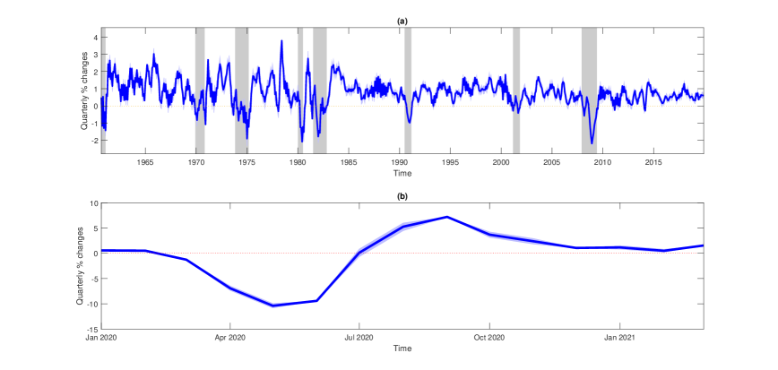
Figure 3: Estimates of monthly Real GDP. Notes: The blue line represents the posterior medians, and the light blue shaded area represents the 68 per cent credible interval. Panel (a) plots the monthly Real GDP estimates for the pre-pandemic period. Panel (b) plots the monthly Real GDP estimates during the pandemic period. The grey shaded areas denote NBER recession dates.

Figure 3 plots the monthly real GDP estimates (posterior median). Panel (a) plots the monthly real GDP estimates during the pre-pandemic period of 1960-2019, and panel (b) plots the monthly estimates during the pandemic period. There are two key features we can draw from Figure 4. First, our monthly real GDP estimates capture all the relevant NBER recessions during the pre-pandemic period. Second, they are consistent with the observed quarterly values produced during the pandemic. This highlights that the proposed precision-based methods are robust to handle samples with extreme outliers.

Next, in figure 4, we plot the SV estimates of real GDP from the MF-BVAR-SV model. The pattern displayed in these SV estimates is consistent with the historical performance of the US economy. For instance, the high volatility associated with the start of the sample can be attributed to the oil price shocks of the 1970-80s. On the other hand, the decline in volatility from the 1980s to the early 2000s is consistent with the timing of the Great Moderation. Therefore, we conclude that the proposed precision-based samplers work well and can handle samples with extreme outliers.

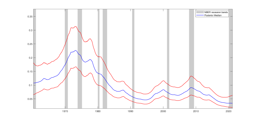
Figure 4: Estimates of the stochastic volatility for Real GDP. Notes: The blue line represents the posterior median estimates, and the red line represents the 68 per cent credible interval. The grey shaded areas denote NBER recession dates.

Another major advantage of producing monthly real GDP estimates from the MF-BVAR-SV model is that we can derive the corresponding monthly output gap via a multivariate Beveridge and Nelson (BN) trend-cycle decomposition from Morley and Wong (2020). Recently, Berger, Morley, and Wong (2021) applied this BN trend-cycle decomposition to a mixed-frequency VAR to nowcast the US output gap. However, their mixed-frequency VAR follows the stacked approach where the model is expressed at the lowest observed frequency. More specifically, their mixed-frequency VAR is essentially a multi-equation U-MIDAS model. Therefore, it can only produce a quarterly measure of the output gap. In contrast, our MF-BVAR-SV model is a state-space mixed-frequency model where we can directly produce a higher-frequency monthly estimate of the output gap. To the best of our knowledge, this is the first study to apply the multivariate BN trend-cycle decomposition within a state-space mixed-frequency VAR framework.

Following Morley and Wong (2020), a finite-order VAR$(p)$ can be represented in the following companion form:

$$(\mathbf{X}_{t}-\boldsymbol{\mu})=\mathbf{F}(\mathbf{X}_{t-1}-\boldsymbol{\mu})+\mathbf{G}\mathbf{e}_{t},$$ (10)

where $\mathbf{X}_{t}$ is vector of the $n$ stationary variables, $\boldsymbol{\mu}$ is a vector of the unconditional means $\mathbf{F}$ is the companion matrix, $\mathbf{G}$ maps the VAR forecast errors to the companion form, and $\mathbf{e}_{t}$ is a vector of forecast errors. Note that the unconditional means can be written as $\boldsymbol{\mu}=(\mathbf{I}_{n}-\mathbf{B}_{1}-\mathbf{B}_{2}-\cdots-\mathbf{B}_{p})^{-1}\mathbf{b}_{0}$, where $\mathbf{B}_{1},\ldots,\mathbf{B}_{p}$ are the VAR coefficient matrices and $\mathbf{\mathbf{b}_{0}}$ is the vector of the intercepts.

From (10), we can derive the cyclical component of the multivariate BN trend-cycle decomposition as

$$\mathbf{c}_{t}^{BN}=-\mathbf{F}(\mathbf{I}-\mathbf{F})^{-1}(\mathbf{X}_{t}-\boldsymbol{\mu}).$$

Figure 5 plots the posterior medians of the cyclical component for the monthly real GDP from the MF-BVAR-SV model. These estimates can be interpreted as a measure of the monthly output gap. For comparison, we also plot two alternative measures of the output gap: the CBO implied output gap and an output gap measure derived using the HP filter obtained from monthly industrial production. Since the CBO implied output gap is a quarterly measure, we assume it is constant across the months for each quarter to produce the figure.

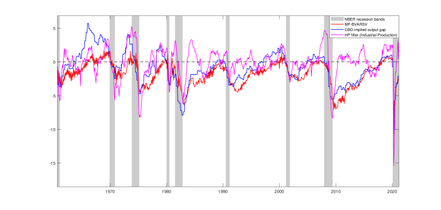
Figure 5: A comparison of monthly output gap estimates. Notes: The red line depicts the posterior median output gap estimates (BN cycle estimates) from our MF-BVAR-SV model. The blue line represents quarterly output gap estimates derived from the CBO. The pink line depicts an output gap measure derived using the HP filter using monthly industrial production. The grey shaded areas denote NBER recession dates.

It is clear from the figure that the measure derived using the HP filter tends to produce large positive output gap estimates at the start of recessions. In contrast, both our monthly output gap estimates and the CBO measure tend to track the NBER recession dates well. However, there are clear differences between them in specific periods. For instance, from mid-2010 to 2019, our output gap estimates tend to be lower than the CBO measure.

A potential explanation for these differences could be the inclusion of financial variables in constructing our output gap measure. According to Coibion, Gorodnichenko, and Ulate (2018), the CBO uses the production function approach to estimate the potential output. In their modelling approach, they only consider five sectors of the economy, and the financial sector is not included. Therefore, the CBO could potentially underestimate the output gap relative to our estimates after the Great Recession since they do not consider financial variables in their model. In addition, our monthly measure provides more timely output gap estimates for policymakers to monitor the economy in real time. This highlights the importance of incorporating higher frequency indicators in the model when deriving an output gap measure.

4.2 A Bayesian Proxy State-Space Mixed-Frequency VAR

In this second application, we show how the proposed mixed-frequency precision-based samplers can be used for structural analysis. Specifically, we extend the Bayesian Proxy (BP)-VAR in Caldara and Herbst (2019) to a mixed-frequency setting, which we denote as MF-BP-VAR. While Caldara and Herbst (2019) estimate both a 4- and 5-equation BP-VAR, here we only consider the endogenous variables from the 5-equation model as that is their preferred model. The five-equation BP-VAR model consists of the federal funds rate (FFR), the log of manufacturing industrial production (IP), the unemployment rate (UE), the log of the producer price index (PPI), and a measure of a corporate spread (Baa corporate bond yield relative to the ten-year treasury constant maturity), which they denote as BAA spread. All five of these variables are observed at the monthly frequency.

We extend this model to a state-space mixed-frequency VAR by including the log of real GDP, observed at the quarterly frequency. Intuitively, real GDP should be a better measure of the real economy than IP. In fact, the share of industrial production to real GDP has been declining since the early 2000s. For instance, the share of industrial production to real GDP was about 71 per cent at the end of 2000, and by the end of 2007, this share had fallen to about 65 per cent.

We consider two MF-BP-VARs with differernt dimensions. In the first case, we estimate a 5-equation MF-BP-VAR without IP; it contains FFR, UE, PPI, BAA spread, and real GDP. For the second case, we consider all 6 variables, including IP . We preserve all the model assumptions as specified in Caldara and Herbst (2019). We estimate the MF-BP-VARs with $p=12$ lags using data from 1994M1-2007M6 (and 1994Q1-2007Q2 for real GDP). Given that the quarterly real GDP variable enters the model in log-level, we impose an inter-temporal constraint similar to that in Schorfheide and Song (2015):

$$y_{t}^{GDP,Q}=\frac{1}{3}(y_{t}^{GDP,m}+y_{t-1}^{GDP,m}+y_{t-2}^{GDP,m}),$$

where $y_{t}^{GDP,Q}$ and $y_{t}^{GDP,m}$ are the observed log quarterly and latent monthly real GDP variable at time $t$, respectively.

Panel (a) of Figure 6 displays the impulse response of the endogenous variables to a one standard deviation monetary shock identified using the 5-equation MF-BP-VAR, and panel (b) displays the corresponding impulse response from the 6-equation MF-BP-VAR, which includes IP. The proxy variable used to identify the monetary policy shock in both models is precisely the same as specified in Caldara and Herbst (2019).

All impulse responses of the monthly endogenous variables from both models display exactly the same dynamics as presented in Caldara and Herbst (2019). This implies that adding quarterly real GDP variable does not change the dynamics of the monthly endogenous variable to a monetary policy shock. However, in both the models, the response of real GDP to a monetary policy shock appears to be muted or subdued compared to the response of IP. For example, in panel (a), the posterior median response of IP falls to a low of $-$0.5 per cent. In contrast, the posterior median response of real GDP tends to be higher than $-$0.2 per cent on average. Therefore, this suggests that the response of IP may be overstating the negative impact of a monetary policy shock on the real economy.

(a)

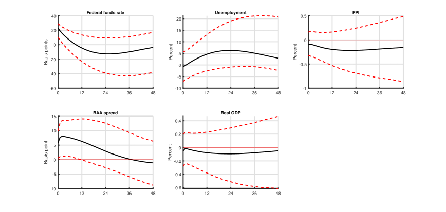
(b)

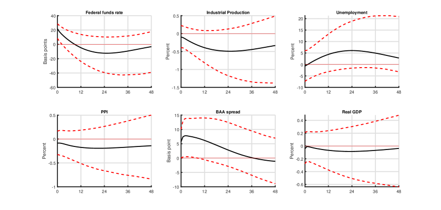
Figure 6: Impulse responses to a monetary policy shock. Notes: Panel (a) reports the impulse response functions generated from the 5-equation MF-BP-VAR. Panel (b) reports the impulse response functions generated from the 6-equation MF-BP-VAR. The solid black line represents the posterior median impulse responses of the specified variable to a one standard deviation monetary policy shock identified via a proxy. The red lines denote the 90 per cent credible intervals.

Table 2 reports the contemporaneous elasticities of FFR to the non-policy variables in both the models and the cumulative elasticities of FFR to all the variables in both models. The majority of the estimates for the monthly endogenous variables are broadly similar to the results presented in Caldara and Herbst (2019).

Table 2: Coefficients in the monetary policy equation.

	5-equation MF-BP-VAR			6-equation MF-BP-VAR
	Median	5th %-tile	95th %-tile	Median	5th %-tile	95th %-tile
Contemporaneous elasticities
Industrial production				0.07	-0.25	0.47
Unemployment	0.14	-1.15	1.71	0.20	-1.29	1.99
PPI inflation	0.11	-0.21	0.52	0.10	-0.25	0.60
BAA spread	-1.44	-4.32	-0.16	-1.43	-4.88	-0.01
Real GDP	-0.04	-0.42	0.34	-0.05	-0.48	0.37
Cumulative elasticities
Federal funds rate	0.96	0.90	1.03	0.96	0.90	1.04
Industrial production				0.00	0.00	0.00
Unemployment	-0.05	-0.18	0.06	-0.06	-0.22	0.08
PPI inflation	0.00	0.00	0.00	0.00	0.00	0.00
BAA spread	-0.24	-0.43	-0.09	-0.21	-0.43	0.00
Real GDP	0.00	0.00	0.00	0.00	0.00	0.00

Notes: The bold entries denote the posterior medians of the contemporaneous elasticities and the cumulative elasticities in the monetary equation identified in the 5-equation and the 6-equation MF-BP-VARs. The associated 5th and 95th percentiles from the posterior distributions are also reported.

The main results we would like to highlight are the contemporaneous and cumulative responses to real GDP. The cumulative response of real GDP for both models is zero. This is consistent with the classical dichotomy theory, where nominal shocks do not affect the real economy in the long run. The contemporaneous responses to real GDP $-$0.04 and $-$0.05 for the 5- and 6-equation MF-BP-VARs, respectively. This suggests that a one standard deviation surprise in real GDP, holding all other things constant, will elicit an immediate monetary policy response of about five basis points. However, this same interpretation cannot be made for IP as estimates imply an inverse relationship between the FFR and IP. Furthermore, this highlights the importance of including real GDP rather than IP as a measure of the real economy.

5 Conclusion

We have introduced two precision-based samplers with hard and soft inter-temporal constraints to draw the low-frequency variables’ missing values within a state-space MF-VAR. The simulation study shows that the proposed methods are more accurate and computationally efficient in estimating the low-frequency variables’ missing values than standard Kalman-filter based methods. We also show how the mixed-frequency precision-based samplers can be applied to two popular empirical macroeconomic applications. Both empirical applications illustrate the importance of incorporating high-frequency indicators in macroeconomic analysis.

For future research, it would be useful to extend the proposed methods to handle real-time datasets with ragged edges. In addition, developing precision-based samplers for dynamic factor models with complex missing data patterns would be another interesting future research direction.

Appendix: Data

This appendix provides details of the 22-variable dataset in the first empirical application. Specifically, Table 3 describes the 22 variables and their transformations. The dataset is sourced from the US FRED database, and the sample covers from 1960M1-2021M3 (and 1960Q1-2021Q1). All the data is transformed to stationarity.

Table 3: The list of variables and the corresponding transformation used in the empirical application.

Variable	Fred Mnemonic	Transformation	Frequency
Real Personal Consumption Expenditures	DPCERA3M086SBEA	100$\Delta$log	Monthly
Real Personal Income	RPI	100$\Delta$log	Monthly
Industrial Production	INDPRO	100$\Delta$log	Monthly
Capacity Utilization: Manufacturing	CUMFNS	$\Delta$	Monthly
Civilian Employment	CE16OV	100$\Delta$log	Monthly
Civilian Unemployment Rate	UNRATE	Level	Monthly
Average Weekly Hours: Manufacturing	AWHMAN	100$\Delta$log	Monthly
Housing Starts: Total New Privately Owned	HOUSTS	100$\Delta$log	Monthly
Personal Consumption Expenditures: Chain Index	PCEPI	100$\Delta^{2}$log	Monthly
Consumer Price Index: All Items	CPIAUCSL	100$\Delta$log	Monthly
PPI: Metals and metal products:	PPICMM	100$\Delta$log	Monthly
PPI: Crude Materials	WPSID61	100$\Delta$log	Monthly
Avg Hourly Earnings: Manufacturing	CES3000000008	100$\Delta^{2}$log	Monthly
Real M2 Money Stock	M2REAL	100$\Delta$log	Monthly
Total Reserves of Depository Institutions	TOTRESNS	100$\Delta$log	Monthly
Commercial and Industrial Loans	BUSLOANS	100$\Delta$log	Monthly
Effective Federal Funds Rate	FEDFUNDS	$\Delta$	Monthly
10-Year Treasury Rate minus 1-Year Treasury Rate	GS10 - GS1	Level	Monthly
Moody’s Seasoned Baa Corporate Bond Yield
minus Moody’s Seasoned Aaa Corporate Bond Yield	BAA-AAA	Level	Monthly
U.S. / U.K. Foreign Exchange Rate	EXUSUKx	100$\Delta$log	Monthly
S&P’s Common Stock Price Index: Composite	S&P 500	100$\Delta$log	Monthly
Real Gross Domestic Product	GDPC1	100$\Delta$log	Quarterly

References

- (1)
- Bańbura, Giannone, and Reichlin (2010) Bańbura, M., D. Giannone, and L. Reichlin (2010): “Large Bayesian vector auto regressions,” Journal of Applied Econometrics, 25(1), 71–92.
- Berger, Morley, and Wong (2021) Berger, T., J. Morley, and B. Wong (2021): “Nowcasting the output gap,” Journal of Econometrics, forthcoming.
- Beyeler and Kaufmann (2021) Beyeler, S., and S. Kaufmann (2021): “Reduced-form factor augmented VAR—Exploiting sparsity to include meaningful factors,” Journal of Applied Econometrics, forthcoming.
- Brave, Butters, and Justiniano (2019) Brave, S. A., R. A. Butters, and A. Justiniano (2019): “Forecasting economic activity with mixed frequency BVARs,” International Journal of Forecasting, 35(4), 1692–1707.
- Brave, Butters, and Kelley (2019) Brave, S. A., R. A. Butters, and D. Kelley (2019): “A new ‘big data’ index of US economic activity,” Economic Perspectives, Federal Reserve Bank of Chicago.
- Caldara and Herbst (2019) Caldara, D., and E. Herbst (2019): “Monetary policy, real activity, and credit spreads: Evidence from Bayesian proxy SVARs,” American Economic Journal: Macroeconomics, 11(1), 157–192.
- Carriero, Clark, and Marcellino (2019) Carriero, A., T. E. Clark, and M. G. Marcellino (2019): “Large Bayesian vector autoregressions with stochastic volatility and non-conjugate priors,” Journal of Econometrics, 212(1), 137–154.
- Carter and Kohn (1994) Carter, C. K., and R. Kohn (1994): “On Gibbs Sampling for State Space Models,” Biometrika, 81, 541–553.
- Chan (2013) Chan, J. C. C. (2013): “Moving Average Stochastic Volatility Models with Application to Inflation Forecast,” Journal of Econometrics, 176(2), 162–172.
- Chan (2017) (2017): “The Stochastic Volatility in Mean Model with Time-Varying Parameters: An Application to Inflation Modeling,” Journal of Business and Economic Statistics, 35(1), 17–28.
- Chan (2020) (2020): “Large Bayesian Vector Autoregressions,” in Macroeconomic Forecasting in the Era of Big Data, ed. by P. Fuleky, pp. 95–125. Springer.
- Chan (2021) (2021): “Minnesota-type adaptive hierarchical priors for large Bayesian VARs,” International Journal of Forecasting, 37(3), 1212–1226.
- Chan, Eisenstat, and Koop (2016) Chan, J. C. C., E. Eisenstat, and G. Koop (2016): “Large Bayesian VARMAs,” Journal of Econometrics, 192(2), 374–390.
- Chan and Jeliazkov (2009) Chan, J. C. C., and I. Jeliazkov (2009): “Efficient simulation and integrated likelihood estimation in state space models,” International Journal of Mathematical Modelling and Numerical Optimisation, 1(1), 101–120.
- Chan, Koop, and Potter (2013) Chan, J. C. C., G. Koop, and S. M. Potter (2013): “A new model of trend inflation,” Journal of Business and Economic Statistics, 31(1), 94–106.
- Chan, Koop, and Potter (2016) (2016): “A bounded model of time variation in trend inflation, NAIRU and the Phillips curve,” Journal of Applied Econometrics, 31(3), 551–565.
- Clark (2011) Clark, T. E. (2011): “Real-time density forecasts from Bayesian vector autoregressions with stochastic volatility,” Journal of Business and Economic Statistics, 29(3), 327–341.
- Clark and Ravazzolo (2015) Clark, T. E., and F. Ravazzolo (2015): “Macroeconomic forecasting performance under alternative specifications of time-varying volatility,” Journal of Applied Econometrics, 30(4), 551–575.
- Coibion, Gorodnichenko, and Ulate (2018) Coibion, O., Y. Gorodnichenko, and M. Ulate (2018): “The cyclical sensitivity in estimates of potential output,” Brookings Papers on Economic Activity, Fall, 434–441.
- Cong, Chen, and Zhou (2017) Cong, Y., B. Chen, and M. Zhou (2017): “Fast simulation of hyperplane-truncated multivariate normal distributions,” Bayesian Analysis, 12(4), 1017–1037.
- Cross, Hou, and Poon (2019) Cross, J., C. Hou, and A. Poon (2019): “Macroeconomic forecasting with large Bayesian VARs: Global-local priors and the illusion of sparsity,” International Journal of Forecasting, 36(3), 899–915.
- Cross and Poon (2016) Cross, J., and A. Poon (2016): “Forecasting structural change and fat-tailed events in Australian macroeconomic variables,” Economic Modelling, 58, 34–51.
- Dimitrakopoulos and Kolossiatis (2020) Dimitrakopoulos, S., and M. Kolossiatis (2020): “Bayesian analysis of moving average stochastic volatility models: modeling in-mean effects and leverage for financial time series,” Econometric Reviews, 39(4), 319–343.
- Doan, Litterman, and Sims (1984) Doan, T., R. Litterman, and C. Sims (1984): “Forecasting and conditional projection using realistic prior distributions,” Econometric reviews, 3(1), 1–100.
- Eckert, Kronenberg, Mikosch, and Neuwirth (2020) Eckert, F., P. Kronenberg, H. Mikosch, and S. Neuwirth (2020): “Tracking economic activity with alternative high-frequency data,” KOF Working Papers, 488, 1–35.
- Fu (2020) Fu, B. (2020): “Is the slope of the Phillips curve time-varying? Evidence from unobserved components models,” Economic Modelling, 88, 320–340.
- Ghysels (2016) Ghysels, E. (2016): “Macroeconomics and the reality of mixed frequency data,” Journal of Econometrics, 193(2), 294–314.
- Grant and Chan (2017a) Grant, A. L., and J. C. C. Chan (2017a): “A Bayesian Model Comparison for Trend-Cycle Decompositions of Output,” Journal of Money, Credit and Banking, 49(2-3), 525–552.
- Grant and Chan (2017b) (2017b): “Reconciling output gaps: Unobserved components model and Hodrick-Prescott filter,” Journal of Economic Dynamics and Control, 75, 114–121.
- Hauber and Schumacher (2021) Hauber, P., and C. Schumacher (2021): “Precision-based sampling with missing observations: A factor model application,” Discussion Papers 11/2021, Deutsche Bundesbank.
- Hou (2020) Hou, C. (2020): “Time-varying relationship between inflation and inflation uncertainty,” Oxford Bulletin of Economics and Statistics, 82(1), 83–124.
- Huber and Feldkircher (2019) Huber, F., and M. Feldkircher (2019): “Adaptive shrinkage in Bayesian vector autoregressive models,” Journal of Business and Economic Statistics, 37(1), 27–39.
- Karlsson (2013) Karlsson, S. (2013): “Forecasting with Bayesian vector autoregressions,” in Handbook of Economic Forecasting, ed. by G. Elliott, and A. Timmermann, vol. 2 of Handbook of Economic Forecasting, pp. 791–897. Elsevier.
- Kaufmann and Schumacher (2019) Kaufmann, S., and C. Schumacher (2019): “Bayesian estimation of sparse dynamic factor models with order-independent and ex-post mode identification,” Journal of Econometrics, 210(1), 116–134.
- Koop (2013) Koop, G. (2013): “Forecasting with medium and large Bayesian VARs,” Journal of Applied Econometrics, 28(2), 177–203.
- Koop and Korobilis (2010) Koop, G., and D. Korobilis (2010): “Bayesian Multivariate Time Series Methods for Empirical Macroeconomics,” Foundations and Trends in Econometrics, 3(4), 267–358.
- Koop, McIntyre, and Mitchell (2020) Koop, G., S. McIntyre, and J. Mitchell (2020): “UK regional nowcasting using a mixed frequency vector auto-regressive model with entropic tilting,” Journal of the Royal Statistical Society: Series A (Statistics in Society), 183(1), 91–119.
- Koop, McIntyre, Mitchell, and Poon (2020) Koop, G., S. McIntyre, J. Mitchell, and A. Poon (2020): “Regional output growth in the United Kingdom: More timely and higher frequency estimates from 1970,” Journal of Applied Econometrics, 35(2), 176–197.
- Litterman (1986) Litterman, R. (1986): “Forecasting With Bayesian Vector Autoregressions — Five Years of Experience,” Journal of Business and Economic Statistics, 4, 25–38.
- Mariano and Murasawa (2003) Mariano, R. S., and Y. Murasawa (2003): “A new coincident index of business cycles based on monthly and quarterly series,” Journal of Applied Econometrics, 18(4), 427–443.
- Mariano and Murasawa (2010) (2010): “A coincident index, common factors, and monthly real GDP,” Oxford Bulletin of Economics and Statistics, 72(1), 27–46.
- McCausland, Miller, and Pelletier (2011) McCausland, W. J., S. Miller, and D. Pelletier (2011): “Simulation smoothing for state-space models: A computational efficiency analysis,” Computational Statistics and Data Analysis, 55(1), 199–212.
- McCracken, Owyang, and Sekhposyan (2020) McCracken, M., M. Owyang, and T. Sekhposyan (2020): “Real-time forecasting and scenario analysis using a large mixed-frequency Bayesian VAR,” International Journal of Central Banking, forthcoming.
- Morley and Wong (2020) Morley, J., and B. Wong (2020): “Estimating and accounting for the output gap with large Bayesian vector autoregressions,” Journal of Applied Econometrics, 35(1), 1–18.
- Polson and Scott (2010) Polson, N. G., and J. G. Scott (2010): “Shrink globally, act locally: Sparse Bayesian regularization and prediction,” Bayesian statistics, 9, 501–538.
- Rue (2001) Rue, H. (2001): “Fast sampling of Gaussian Markov random fields with applications,” Journal of the Royal Statistical Society: Series B (Methodological), 63(2), 325–338.
- Rue and Held (2005) Rue, H., and L. Held (2005): Gaussian Markov Random Fields: Theory and Applications. CRC press.
- Schorfheide and Song (2015) Schorfheide, F., and D. Song (2015): “Real-time forecasting with a mixed-frequency VAR,” Journal of Business and Economic Statistics, 33(3), 366–380.
- Zhang, Chan, and Cross (2020) Zhang, B., J. C. C. Chan, and J. L. Cross (2020): “Stochastic volatility models with ARMA innovations: An application to G7 inflation forecasts,” International Journal of Forecasting, 36(4), 1318–1328.