Risk bounds for aggregated shallow neural networks using Gaussian prior

Abstract

Analysing statistical properties of neural networks is a central topic in statistics and machine learning. However, most results in the literature focus on the properties of the neural network minimizing the training error. The goal of this paper is to consider aggregated neural networks using a Gaussian prior. The departure point of our approach is an arbitrary aggregate satisfying the PAC-Bayesian inequality. The main contribution is a precise nonasymptotic assessment of the estimation error appearing in the PAC-Bayes bound. We also review available bounds on the error of approximating a function by a neural network. Combining bounds on estimation and approximation errors, we establish risk bounds which are sharp enough to lead to minimax rates of estimation over Sobolev smoothness classes.

1 Introduction

Neural networks are the most widely used parameterised functions for solving machine learning tasks. The parameters of the neural network are then learned from data. Assessing the error of the learned network on new, unobserved examples is a central topic in statistics and learning theory (Bartlett et al., 2021; Fan et al., 2021). The most popular approach for estimating the parameters of the network from data, referred to as weights and biases, is the minimization of the (regularized) training error. This is usually done by the stochastic gradient descent, or a version of it. Risk bounds for these networks are based on Vapnik-Chervonenkis dimension (Bartlett et al., 1998; Anthony and Bartlett, 1999; Bartlett et al., 2019). Even for simple networks containing only one hidden layer, these risk bounds are rather involved (Xie et al., 2017; Zhong et al., 2017; Cao and Gu, 2019; Ba et al., 2020).

A well-known alternative to minimizing the regularized training error is to use a prediction rule based on a posterior distribution. Typical example is the network obtained by sampling its weights from the posterior, or the convex combination of the networks averaged using the posterior distribution. Surprisingly, little is known about risk bounds of posterior-based prediction rules in the context of neural networks. The goal of the present work is to do the first step in filling this gap by focusing on one-hidden-layer feedforward neural networks and Gibbs posteriors using Gaussian prior. An attractive feature of posterior-based methods is that their analysis can be carried out using the PAC-Bayes theory (McAllester, 1999, 2003) as a substitute to the Vapnik-Chervonenkis dimension or the Rademacher complexity. We refer the reader to (Catoni, 2007; Guedj, 2019; Alquier, 2021) for a comprehensive account of the PAC-Bayesian approach in statistics and learning.

PAC-Bayes theory has been already used in the framework of neural networks, mainly for providing data-driven bounds on the generalisation error of trained (stochastic) networks and prior selection based on these bounds (Rivasplata et al., 2018; Lever et al., 2013; Dziugaite and Roy, 2017; Neyshabur et al., 2017; Zhou et al., 2019; Letarte et al., 2019; Biggs and Guedj, 2021; Perez-Ortiz et al., 2021a, b). In this paper, we take a different route and propose to use in-expectation PAC-Bayes bounds for investigating the risk (or, the expected excess loss) of aggregated neural networks. To be more specific, let $\mathcal{F}_{\mathsf{W}}:=\{f_{\bm{w}},{\bm{w}}\in{\mathsf{W}}\}$ be a parametric class of prediction rules, with a parameter $\bm{w}$ lying in a measurable space $({\mathsf{W}},\mathscr{W})$. One can think of $\mathcal{F}_{\mathsf{W}}$ as a set of neural networks with a given architecture and of $\bm{w}$ as the vector of the weights and biases. Assume we are given a sample of size $n$ independently drawn from an unknown distribution $\bf P$, and we wish to “aggregate” elements of $\mathcal{F}_{\mathsf{W}}$ to obtain a prediction rule $\widehat{f}_{n}$ that mimics the Bayes predictor $f_{\mathbf{P}}$. This means that for a prescribed loss function $\ell(\cdot,\cdot)$ taking real values, we wish $\ell(\widehat{f}_{n},f_{\mathbf{P}})$ to be small. It turns out that under some general assumptions, for a given prior distribution $\pi$ on $\mathsf{W}$ and a temperature parameter $\beta>0$, there exists an aggregate $\widehat{f}_{n}$ such that

$$\mathbf{E}[\ell(\widehat{f}_{n},f_{\mathbf{P}})]\leq C_{\textsf{PB}}\inf_{p}\bigg{\{}\int_{\mathsf{W}}\ell(f_{\bm{w}},f_{\mathbf{P}})\,p(d\bm{w})+\frac{\beta}{n}\,D_{\textsf{KL}}(p||\pi)\bigg{\}},$$ (1)

where $C_{\textsf{PB}}$ is some constant and the infimum is over all probability distributions $p$ over $\mathsf{W}$. We say then that $\widehat{f}_{n}$ satisfies a PAC-Bayes inequality in-expectation. For regression with fixed design, the Gibbs-posterior mean was shown to satisfy (1) with $C_{\textsf{PB}}=1$ in (Leung and Barron, 2006) for Gaussian noise, and in (Dalalyan and Tsybakov, 2007) for more general noise distributions. In some other problems, including the random design regression and the density estimation, similar bounds were established for the mirror averaging (Yuditskii et al., 2005; Juditsky et al., 2008). PAC-Bayes bounds with $C_{\textsf{PB}}>1$ for the prediction rule obtained by randomly drawing $\bm{w}$ from the Gibbs posterior were proved in (Catoni, 2007; Alquier and Biau, 2013). The recent papers (Biggs and Guedj, 2021; Fortier-Dubois et al., 2021) studied the problem of aggregation of neural networks with sign activation.

In the present work, we elaborate on (1) to get a tractable risk bound when $\mathcal{F}_{\mathsf{W}}$ is the set of neural networks with a single hidden layer. The tractability here should be understood as the property of showing clearly the dependence on the important problem characteristics (sample-size, input and output dimensions) and those of the learning algorithm (variances of the prior distribution, number of hidden layers, properties of the activation functions). Our first main contribution stated in Theorem 2 is a tractable risk bound formulated as an oracle inequality. To our knowledge, this inequality is sharper and easier to deal with than its counterparts for the training error minimizing shallow networks. To show potential implications of this oracle inequality, we combine it with known approximation bounds when the Bayes predictor lies in a Sobolev ball. Interestingly, we show that a proper choice of the width of the hidden layer and the variances of the prior leads to minimax optimal rates of convergence, up to logarithmic factors. More specifically, for the Sobolev ball $W^{r}_{2}([0,1]^{D_{0}})$ of smoothness $r$ and input dimension $D_{0}$, we obtain in Theorem 6 the rate $n^{-{2r}/{(2r+D_{0})}}\log^{2}n$ for a specific class of sigmoid activation functions. A similar result is obtained for the ReLU activation as well, but with a slightly slower rate $n^{-{2\bar{r}}/{(2\bar{r}+D_{0}+1)}}$ (up to a polylogarithmic factor) for any $\bar{r}<r$.

The rest of the paper is organized as follows. In Section 2, we define the generic PAC-Bayesian framework and instantiate it in the setting of shallow neural networks. In Section 3, we state the main oracle bound for shallow neural networks with a Gaussian prior. Section 4 provides examples of statistical problems where PAC-Bayesian bounds of type (1) are available. Section 5 is devoted to a selective review of the literature on approximation properties of neural networks with bounded (sigmoid) and unbounded (ReLU) activation functions. Finally, Section 6 contains the upper bounds on the worst-case risk which are nearly minimax rate-optimal in the case of sigmoid activation. Some concluding remarks are provided in Section 7. Technical proofs are deferred to the appendices.

2 Preliminaries and notation

In this section, we set the general framework of the PAC-Bayesian bound that will be the starting point of our work. We then instantiate it in the specific case of neural networks.

2.1 General framework and PAC-Bayesian type bounds

Let $(\mathcal{Z},\mathscr{A})$ be a measurable space. We observe one realisation of the random vector $\mathbf{Z}^{n}=(Z_{1},\dots,Z_{n})\in\mathcal{Z}^{n}$ drawn from an unknown distribution $\mathbf{P}$ on $(\mathcal{Z}^{n},\mathscr{A}^{\otimes n})$. We denote by $\|\bm{x}\|_{2}$ the Euclidean norm of the vector $\bm{x}$ of an Euclidean space. Let $\mathcal{X}\subset\mathbb{R}^{D_{0}}$, $D_{0}\geq 1$, be a Borel set and let $\mu$ be a $\sigma$-finite measure on $\big{(}\mathcal{X},\mathscr{B}(\mathcal{X})\big{)}$ such that $M_{2}^{2}=D_{0}^{-1}\int_{\mathcal{X}}\|\bm{x}\|_{2}^{2}\,\mu(d\bm{x})<+\infty$. In the sequel, we denote by $\mathbb{L}_{q}(\mu)$, $q\in[1,\infty)$, the set of all the functions $f:\mathcal{X}\to\mathbb{R}^{D_{2}}$ such that $\int_{\mathcal{X}}\|f(\bm{x})\|_{2}^{q}\,\mu(d\bm{x})<\infty$. Let $\mathcal{P}_{\mathsf{W}}$ be the space of all probability measures on ${\mathsf{W}}$ and let

$$\mathcal{P}_{1}(\mathcal{F}_{\mathsf{W}})=\Big{\{}p\in\mathcal{P}_{\mathsf{W}}:\int_{\mathsf{W}}\|f_{\bm{w}}(\bm{x})\|_{2}\,p(d{\bm{w}})<\infty,\quad\text{for all}\quad x\in\mathcal{X}\Big{\}}.$$ (2)

We consider the problem of estimating a function $f_{\mathbf{P}}\in\mathbb{L}_{2}(\mu)$. At this stage, one may think of $f_{\mathbf{P}}$ as the multidimensional regression function when $\mathcal{Z}=\mathcal{X}\times\mathbb{R}^{D_{2}}$, the Bayes classifier when $\mathcal{Z}=\mathcal{X}\times\{-1,1\}$ or the density of observations when $\mathcal{Z}=\mathcal{X}$ (in the last two cases $D_{2}=1$). A common approach in statistics and statistical learning is to use a parametric set $\mathcal{F}_{\mathsf{W}}:=\{f_{\bm{w}},{\bm{w}}\in{\mathsf{W}}\}\subset\mathbb{L}_{2}(\mu)$, indexed by a measurable set $\mathsf{W}\subset\mathbb{R}^{d}$, for some $d\in\mathbb{N}$, for constructing an estimator of $f_{\mathbf{P}}$. Instances of this approach are the empirical risk minimizer, the Bayesian posterior mean, the exponentially weighted aggregate, etc. The quality of an estimator $\widehat{f}_{n}$ of $f_{\mathbf{P}}$ is measured by means of a loss function $\ell:\mathbb{L}_{2}(\mu)\times\mathbb{L}_{2}(\mu)\mapsto\mathbb{R}_{+}$; an estimator $\widehat{f}_{n}$ is good if its risk

$$\mathbf{E}_{\mathbf{P}}\big{[}\ell\big{(}\widehat{f}_{n}(\mathbf{Z}^{n}),f_{\mathbf{P}}\big{)}\big{]}=\int_{\mathcal{Z}^{n}}\ell\big{(}\widehat{f}_{n}(\mathbf{z}),f_{\mathbf{P}}\big{)}\,\mathcal{P}(d\mathbf{z})$$ (3)

is small. A widespread choice of the loss function, used throughout this paper except in Section 4, is the squared $\ell_{2}$-norm $\ell(g,h)=\|g-h\|^{2}_{\mathbb{L}_{2}(\mu)}=\int_{\mathcal{X}}\|g(\bm{x})-h(\bm{x})\|_{2}^{2}\,\mu(d\bm{x})$, $\forall g,h\in\mathbb{L}_{2}(\mu)$.

We say that the estimator $\widehat{f}_{n}$ satisfies the PAC-Bayesian bound with prior $\pi\in\mathcal{P}_{1}(\mathcal{F}_{\mathsf{W}})$ and temperature parameter $\beta>0$, if (1) is satisfied (where the infimum in the right hand side is over all $p$ in $\mathcal{P}_{1}(\mathcal{F}_{\mathsf{W}})$). If $C_{\textsf{PB}}=1$, the bound is called exact or sharp. When the loss function is the squared $\mathbb{L}_{2}$-norm, the PAC-Bayesian bound reads as

$$\mathbf{E}_{\mathbf{P}}[\|\widehat{f}_{n}-f_{\mathbf{P}}\|_{\mathbb{L}_{2}}^{2}]\leq C_{\textsf{PB}}\inf_{p\in\mathcal{P}_{1}(\mathcal{F}_{\mathsf{W}})}\bigg{\{}\int_{\mathsf{W}}\|f_{\bm{w}}-f_{\mathbf{P}}\|_{\mathbb{L}_{2}(\mu)}^{2}\,p(d\bm{w})+\frac{\beta}{n}\,D_{\textsf{KL}}(p||\pi)\bigg{\}}.$$ (4)

2.2 Shallow neural networks

In the rest of this section, we provide more details on the notations and assumptions that will stand when we estimate $f_{\mathbf{P}}$ by aggregation of neural networks. We consider the class of networks with a single hidden layer and denote by $D_{1}$ the number of units in this layer.

In order to merge weights and biases of a neural network, we note $\bm{x}=(1,x_{1},\dots,x_{D_{0}-1})^{\top}\in\mathcal{X}$. The set ${\mathsf{W}}$ of the weights of a neural network can be divided into the weights of the hidden layer, $\bm{w}_{1}$, and the weights of the output layer, $\bm{w}_{2}$ so that $\bm{w}_{1}\in\mathbb{R}^{D_{0}\times D_{1}}$ and $\bm{w}_{2}\in\mathbb{R}^{D_{1}\times D_{2}}$. Therefore, $\bm{w}=(\bm{w}_{1},\bm{w}_{2})^{\top}$ can be seen as an element of $\mathbb{R}^{d}$ with the overall dimension $d=D_{0}D_{1}+D_{1}D_{2}$. The neural network parametrized by $\bm{w}$ has the form:

$$f_{\bm{w}}(\bm{x})=\bm{w}_{2}^{\top}\bar{\sigma}(\bm{w}^{\top}_{1}\bm{x})\in\mathbb{R}^{D_{2}},\ \forall\bm{x}\in\mathbb{R}^{D_{0}}\quad\text{with}\quad\bar{\sigma}:\bm{x}\in\mathbb{R}^{D_{1}}\mapsto\begin{bmatrix}\sigma(x_{1})\\ \vdots\\ \sigma(x_{D_{1}})\end{bmatrix}\in\mathbb{R}^{D_{1}},$$ (5)

where $\sigma:\mathbb{R}\to\mathbb{R}$ is a scalar activation function. In the next sections, we will consider both the case of bounded and unbounded activation functions in order to cover most of the usual ones. We refer to the bounded case by means of the following assumption.

Assumption ($\sigma$-B).

The function $\sigma$ is bounded by $M_{\sigma}$, i.e, $|\sigma(u)|\leq M_{\sigma}$ for all $u\in\mathbb{R}$.

Let us stress that only some of our results require ($\sigma$-B). However, all our results will require the Lipschitz assumption stated below, which is satisfied by sigmoid functions as well as piecewise continuous functions (including ReLU). Without loss of generality, we will assume that the Lipschitz constant is equal to one.

Assumption ($\sigma$-L).

For every pair of real numbers $(u,u^{\prime})$, we have $|\sigma(u)-\sigma(u^{\prime})|\leq|u-u^{\prime}|$.

2.3 Spherical Gaussian prior distribution

The prior distribution $\pi$ defined in the PAC-Bayesian framework can be interpreted as the initial distribution of the weights, or as a regulariser. We focus in this paper on the most natural choice of prior, the Gaussian distribution. Recall that the weights of a neural network are split into two groups: the weights $\bm{w}_{1}$ of the hidden layer and the weights $\bm{w}_{2}$ of the output layer. To take into account their different roles we assume the distribution over $\bm{w}$ is a product of two spherical Gaussians with different variances.

Assumption ($\mathcal{N}$).

The prior $\pi$ satisfies $\pi=\pi_{1}\otimes\pi_{2}=\mathcal{N}(0,\rho^{2}_{1}\mathbf{I}_{D_{0}D_{1}})\otimes\mathcal{N}(0,\rho^{2}_{2}\mathbf{I}_{D_{1}D_{2}})$.

We refer to $\pi_{1}$ and $\pi_{2}$ as the distribution of the hidden layer and the output layer respectively.

3 Oracle inequalities for networks with one hidden layer and Gaussian prior

In this section, we first derive a bound for the risk of the estimator $\widehat{f}_{n}$ when the prior has an arbitrary centered Gaussian distribution, and subsequently provide an oracle inequality for a carefully chosen Gaussian prior. Let $\bar{\bm{w}}\in\mathsf{W}$ be any value of the parameter. Using the triangle inequality, in conjunction with the fact that $\sqrt{(a+b)^{2}+c^{2}}\leq a+\sqrt{b^{2}+c^{2}}$, one can infer from (4) that

$$\Big{(}C_{\mathsf{PB}}^{-1}\,\mathbf{E}_{\mathbf{P}}\big{[}\|\widehat{f}_{n}-f_{\mathbf{P}}\|_{\mathbb{L}_{2}(\mu)}^{2}\big{]}\Big{)}^{1/2}\leq\|f_{\bar{\bm{w}}}-f_{\mathbf{P}}\|_{\mathbb{L}_{2}(\mu)}+\textup{Rem}_{n}(\bar{\bm{w}})^{1/2},$$ (6)

with the remainder term given by

$$\textup{Rem}_{n}(\bar{\bm{w}})\triangleq\inf_{p\in\mathcal{P}_{1}(\mathcal{F}_{\mathsf{W}})}\bigg{\{}\int_{\mathsf{W}}\|f_{\bm{w}}-f_{\bar{\bm{w}}}\|_{\mathbb{L}_{2}(\mu)}^{2}\,p(d\bm{w})+\frac{\beta}{n}\,D_{\textsf{KL}}(p||\pi)\bigg{\}}.$$ (7)

Considering $f_{\bar{\bm{w}}}$ as an approximator of $f_{\mathbf{P}}$, the right hand side of (6) can be seen as the sum of the approximation error $\|f_{\bar{\bm{w}}}-f_{\mathbf{P}}\|_{\mathbb{L}_{2}(\mu)}$ and the estimation error $\textup{Rem}_{n}(\bar{\bm{w}})$. The main goal of this paper is to analyze this estimation error and then to combine it with available bounds on the approximation error. Our approach will consist in replacing the infinimum over all measures $p$ by the infinimum over Gaussian distributions, for which mathematical derivations are considerably simpler.

It is well-known (see, for example, (McAllester, 2003; Alquier, 2009; Guedj, 2019)) that for a fixed $\bar{\bm{w}}$, the infinimum in (7) is attained by the Gibbs distribution

$$p^{*}(d\bm{w})\propto\exp\Big{\{}-\frac{n}{\beta}\|f_{\bm{w}}-f_{\bar{\bm{w}}}\|_{\mathbb{L}_{2}(\mu)}^{2}\Big{\}}\pi(d\bm{w}).$$ (8)

Furthermore in this case,

$$\textup{Rem}_{n}(\bar{\bm{w}})=-\frac{\beta}{n}\,\log\int_{\mathsf{W}}\exp\Big{\{}-\frac{n}{\beta}\|f_{\bm{w}}-f_{\bar{\bm{w}}}\|_{\mathbb{L}_{2}(\mu)}^{2}\Big{\}}\pi(d\bm{w}).$$ (9)

This expression is often referred to as the free energy. The content of the rest of this section can be seen as leveraging the variational formulation (7) for obtaining user-friendly upper bounds.

Proposition 1.

Let ($\sigma$-L) and ($\mathcal{N}$) be satisfied. Recall that $d=D_{0}D_{1}+D_{1}D_{2}$ is the number of weights of the neural network and $n$ is the sample size.

• If ($\sigma$-B) holds true, then

  $$\textup{Rem}_{n}(\bar{\bm{w}})\leq\frac{\beta}{2n}\bigg{\{}\frac{\|\bar{\bm{w}}_{1}\|_{\mathsf{F}}^{2}}{\rho_{1}^{2}}+\frac{\|\bar{\bm{w}}_{2}\|_{\mathsf{F}}^{2}}{\rho_{2}^{2}}+d\log\left(1+\frac{2n(A_{1}\rho_{1}^{2}+A_{2}\rho_{2}^{2})}{d\beta}\right)\bigg{\}}$$ (10)

  where $A_{1}=D_{0}D_{1}M_{2}^{2}\|\bar{\bm{w}}_{2}\|^{2}_{\mathsf{F}}$ and $A_{2}=D_{1}D_{2}\mu(\mathcal{X})M_{\sigma}^{2}$.

• If the activation function is unbounded but vanishes at the origin, then

  $$\textup{Rem}_{n}(\bar{\bm{w}})\leq\frac{\beta}{2n}\bigg{\{}\frac{\|\bar{\bm{w}}_{1}\|_{\mathsf{F}}^{2}}{\rho_{1}^{2}}+\frac{\|\bar{\bm{w}}_{2}\|_{\mathsf{F}}^{2}}{\rho_{2}^{2}}+2d\log\left(1+\frac{n(A_{1}\rho_{1}^{2}+A_{2}^{\prime}\rho_{2}^{2}+A_{3}^{\prime}\rho_{1}^{2}\rho_{2}^{2})}{d\beta}\right)\bigg{\}}$$ (11)

  where $A^{\prime}_{2}=\bar{M}_{2}^{2}\|\bar{\bm{w}}_{1}\|_{\mathsf{F}}^{2}D_{2}$ and $A^{\prime}_{3}=M_{2}^{2}D_{0}D_{2}$.

Quantities $A_{1}$, $A_{2}$, $A_{2}^{\prime}$ and $A_{3}^{\prime}$ defined in the proposition, are independent of the sample size $n$, the temperature parameter $\beta$ and the variances $\rho_{1}$ and $\rho_{2}$ of the prior distribution, but they are dimension dependent.

There are two dual ways of drawing statistical insights from the above bounds on the estimation error. The first way is to consider $\tau_{1},\tau_{2}$ and $D_{1}$ as “tuning parameters” of the algorithm, and to prove that for a suitable choice of these parameters the predictor $\widehat{f}_{n}$ is optimal. This line of thought is further developed in Section 6 below. The second way of interpreting the obtained bound is to see which functions are well estimated by $\widehat{f}_{n}$ based on $\tau_{1},\tau_{2}$ and $D_{1}$. This leads to the following result.

Theorem 2.

Let $\widehat{f}_{n}$ be a method of aggregation of shallow neural networks $\mathcal{F}_{\mathsf{W}}=\{f_{\bm{w}}(\bm{x})=\bm{w}_{2}^{\top}\bar{\sigma}(\bm{w}_{1}^{\top}\bm{x}):\bm{w}_{1}\in\mathbb{R}^{D_{0}\times D_{1}};\bm{w}_{2}\in\mathbb{R}^{D_{1}\times D_{2}}\}$, based on a prior distribution $\pi$, satisfying PAC-Bayes bound (4). Let Assumptions ($\sigma$-L) and ($\mathcal{N}$) be satisfied. Then, for $B_{\ell}=\rho_{\ell}\sqrt{2D_{\ell-1}D_{\ell}}$, $\ell=1,2$, we have

$$\Big{(}C_{\mathsf{PB}}^{-1}\mathbf{E}_{\mathbf{P}}\big{[}\|\widehat{f}_{n}-f_{\mathbf{P}}\|_{\mathbb{L}_{2}(\mu)}^{2}\big{]}\Big{)}^{1/2}\leq\inf_{\begin{subarray}{c}\|\bm{w}_{1}\|_{\mathsf{F}}\leq B_{1}\\ \|\bm{w}_{2}\|_{\mathsf{F}}\leq B_{2}\end{subarray}}\|f_{\bar{\bm{w}}}-f_{\mathbf{P}}\|_{\mathbb{L}_{2}(\mu)}+\Big{\{}\frac{\beta d}{n}\log\Big{(}3+\frac{nE}{d\beta}\Big{)}\Big{\}}^{1/2},$$ (12)

where the constant E is defined by

$$E=\begin{cases}3B_{2}^{2}(B_{1}^{2}M_{2}^{2}+\mu(\mathcal{X})M_{\sigma}^{2}),&\text{if $\sigma$ satisfies \lx@cref{creftypecap~refnum}{ass:bounded}},\\ 3B_{1}^{2}B_{2}^{2}(M_{2}^{2}+\bar{M}_{2}^{2}/D_{1}),&\text{if $\sigma$ is unbounded but $\sigma(0)=0$}.\end{cases}$$ (13)

An important consequence of this result is that the estimation error, upper bounded by the second term in (12), is of order $\sqrt{D_{1}/n}$ (we assume that the input and the output dimensions are fixed and neglect logarithmic factors). This is similar to many non-parametric estimation methods. For instance, if the regression function is estimated by a histogram with $K$ bins, the estimation error is generally of order $\sqrt{K/n}$. Thus, the number of units in the hidden layer of a neural network plays the same role as the number of bins in a histogram. This parameter $D_{1}$ has to be chosen carefully, in order to control both the approximation error and the estimation error.

4 Examples of application

PAC-Bayes inequality is stated in (1) in a rather general form. In this section, we provide examples of learning problems and learning algorithms for which a version of (1) is satisfied.

4.1 Fixed design regression

Regression with deterministic design and additive errors is often used in nonparametric modeling. In the case of Gaussian errors, it corresponds to the observations

$$\bm{Z}_{i}=f_{\mathbf{P}}(\bm{x}_{i})+\sigma\bm{\xi}_{i},\qquad\bm{\xi}_{i}\stackrel{{\scriptstyle\textup{iid}}}{{\sim}}\mathcal{N}(0,\mathbf{I}_{D_{2}}),\quad i=1,\ldots,n,$$ (14)

where $\bm{x}_{1},\dots,\bm{x}_{n}$ are given deterministic points and $\mathcal{Z}=\mathbb{R}^{D_{2}}$. In this case, the measure $\mu$ is the empirical uniform distribution: $\mu=\frac{1}{n}\sum_{i=1}^{n}\delta_{\bm{x}_{i}}$.

There are many results of type (1) in the literature for regression with fixed design. In particular, (Leung and Barron, 2006; Dalalyan and Tsybakov, 2007, 2008; Dalalyan and Salmon, 2012; Dalalyan and Tsybakov, 2012b; Dalalyan, 2020; Rigollet and Tsybakov, 2012) established a PAC-Bayesian bound for the exponentially weighted aggregate defined by $\widehat{f}_{n}(\mathbf{Z},\bm{x})=\int_{\mathsf{W}}f_{\bm{w}}(\bm{x})\,\widehat{\theta}_{n,\bm{w}}(\mathbf{Z})\,\pi(d{\bm{w}})$ with

$$\widehat{\theta}_{n,\bm{w}}(\mathbf{Z}) =\frac{\exp\{-\frac{1}{\beta}\sum_{i=1}^{n}\|\bm{Z}_{i}-f_{\bm{w}}(\bm{x}_{i}))\|_{2}^{2}\}}{\int_{\mathsf{W}}\exp\{-\frac{1}{\beta}\sum_{i=1}^{n}\|\bm{Z}_{i}-f_{\bm{u}}(\bm{x}_{i}))\|_{2}^{2}\}\,\pi(d\bm{u})}.$$ (15)

Note that $\bm{w}\mapsto\widehat{\theta}_{n,{\bm{w}}}$ is a probability density on $(\mathsf{W},\pi)$, often referred to as posterior density. For precise conditions under which the exponentially weighted aggregate $\widehat{f}_{n}(\mathbf{Z},\bm{x})$ satisfies PAC-Bayes bound (4), the interested reader is referred to the papers mentioned above.

4.2 Random design regression

In the setting of iid observations, sharp PAC-Bayes inequality is valid for the mirror averaging (MA) estimator (Juditsky et al., 2008; Dalalyan and Tsybakov, 2012a; Gerchinovitz, 2013). We define the estimator in the case of regression with random design, and briefly mention below that similar results hold for density estimation and classification. Interested reader is referred to (Juditsky et al., 2008; Dalalyan and Tsybakov, 2012a) for more detailed and comprehensive account on the topic. Note that similar inequalities are obtained for the $Q$-aggregation procedure (Dai et al., 2012; Lecué and Rigollet, 2014).

The regression problem writes as in the previous example

$$\bm{Y}_{i}=f_{\mathbf{P}}(\bm{X}_{i})+\sigma\bm{\xi}_{i},\qquad\bm{\xi}_{i}\perp\perp\bm{X}_{i},\quad i=1,\dots,n,$$ (16)

with $\mathcal{Z}=\mathcal{X}\times\mathcal{Y}$, $\mathcal{X}\subset\mathbb{R}^{D_{0}},\;\mathcal{Y}\subset\mathbb{R}^{D_{2}}$ and $(\bm{X}_{i},\bm{Y}_{i})$ being iid. The natural choice of the measure $\mu$ here is the marginal distribution of $\bm{X}_{i}$ over $\mathcal{X}$.

The mirror averaging procedure satisfying (1) takes the form

$$\widehat{f}_{n}(\mathbf{Z},x)=\int_{\mathsf{W}}f_{\bm{w}}(x)\,\widehat{\theta}_{n,\bm{w}}^{\textup{MA}}(\mathbf{Z})\,\pi(d{\bm{w}})=\frac{1}{n+1}\sum_{m=0}^{n}\int_{\mathsf{W}}f_{\bm{w}}(x)\,\widehat{\theta}_{m,{\bm{w}}}(\mathbf{Z})\,\pi(d{\bm{w}})$$ (17)

with $\widehat{\theta}_{0,{\bm{w}}}=1$ and

$$\theta_{n,\bm{w}}^{\textup{MA}}(\mathbf{Z})=\frac{1}{n+1}\sum_{m=0}^{n}\frac{\exp\{-\frac{1}{\beta}\sum_{i=1}^{m}Q(\bm{Z}_{i},f_{\bm{w}})\}}{{\int_{\mathsf{W}}\exp\{-\frac{1}{\beta}\sum_{i=1}^{m}Q(\bm{Z}_{i},f_{\widetilde{\bm{w}}})\}\,\pi(d\widetilde{\bm{w}})}},$$ (18)

where $Q:\mathcal{Z}\times\mathbb{L}_{2}(\mu)\mapsto\mathbb{R}$ is a mapping satisfying some assumptions under which the minimizer of the loss $\ell:g\mapsto\ell(g,f)$ coincides with the minimizer of $g\mapsto\mathbf{E}_{\mathbf{P}}\left[Q(\mathbf{Z},g)\right]$. In the case of regression, the mirror averaging estimator can be evaluated with the $\ell_{2}$-norm such that in (18), the function $Q$ is given by $Q(\bm{Z}_{i},f_{\bm{w}})=\|\bm{Y}_{i}-f_{\bm{w}}(\bm{X}_{i})\|_{2}^{2}$.

4.3 Density estimation

Consider the case where the elements of $\mathbf{Z}^{n}=(\bm{Z}_{1},\dots,\bm{Z}_{n})\in\mathcal{Z}^{n}$ are iid random variables drawn from a distribution having $f_{\mathbf{P}}$ as density with respect to a measure $\mu$. We aim to estimate $f_{\mathbf{P}}$ and measure the risk using the squared integrated error

$$\ell(\widehat{f}_{n},f)=\|\widehat{f}_{n}-f\|^{2}_{\mathbb{L}_{2}(\mu)}=\int_{\mathcal{X}}\big{(}\widehat{f}_{n}(\bm{x})-f(\bm{x})\big{)}^{2}\mu(d\bm{x})$$ (19)

such that the mapping $Q$ in (18) can by defined by $Q(\bm{x},g)=\|g\|^{2}_{\mathbb{L}_{2}(\mu)}-2g(\bm{x})$.

4.4 Classification for $\Phi$-risk

Consider the binary classification problem with $\mathcal{Z}=\mathbb{R}^{D_{0}}\times\{-1,+1\}$ and assume that such that $\mathbf{Z}^{n}=((X_{1},Y_{1}),\dots,(X_{n},Y_{n}))$ are iid observations drawn from a distribution $\mathbf{P}$ on $\mathcal{Z}$. For a twice differentiable convex function $\Phi$, the $\Phi$-risk of a classifier $g:\mathbb{R}^{D_{0}}\to\{-1,+1\}$ is given by $R_{\mathbf{P}}^{\Phi}[g]=\mathbf{E}_{\mathbf{P}}[\Phi(-Yg(X))]$. In this setting, the loss function can be defined as $\ell(g,f)=R_{\mathbf{P}}^{\Phi}[g]-R_{\mathbf{P}}^{\Phi}[f]$, and the MA estimator given by (17)–(18) can be used with the function $Q(z,g)=\Phi(-yg(x))$.

5 Approximation bounds

The goal of this section is to review existing bounds on the approximation error of neural networks for different classes of functions. We are particularly interested in shallow networks and in bounds having explicit dependence on the width of the hidden layer. The main question of interest is the assessment of the distance between a given function and it’s best approximation by a one-hidden-layer network with $D_{1}$ units in the hidden layer. Our focus is on Lipchtiz activation functions such as logistic, tanh, ReLU or quadratic (for bounded inputs). Because of major differences between the sigmoidal and ReLU activation functions, these two cases will be presented separately.

5.1 Bounds for sigmoidal activation functions

For sigmoid activation functions we distinguish the probabilistic approach (Barron, 1993; Delyon et al., 1995; Maiorov and Meir, 2000; Maiorov, 2006) from the deterministic and constructive approaches (Mhaskar and Micchelli, 1994; Petrushev, 1998; Burger and Neubauer, 2001; Cao et al., 2008; Costarelli and Spigler, 2013a, b). For the set of univariate locally $\alpha$-Hölder continuous functions with $\alpha\in(0,1]$, the constructive approach of (Cao et al., 2008) leads to an approximation error of order of $D_{1}^{-\alpha}$ in $\ell_{\infty}$-norm. For $\alpha>1$, (Costarelli and Spigler, 2013a) shows that the approximation error is $O(D_{1}^{-1})$ both for univariate and multivariate functions.

For other classes of functions, a common feature of the results is the requirement of the existence of some type of integral transform (e.g., Fourier, Radon, wavelet) of the function $f_{\mathbf{P}}$. Each transform is tailored to a different “smoothness” class. An early example is the constructive approach from (Mhaskar and Micchelli, 1994) that focused on $2\pi$-periodic functions from $\mathbb{L}_{2}([-\pi,\pi]^{D_{0}})$ with absolutely convergent Fourier series. For such functions, the approximation error is shown to be $O(D_{1}^{-1/2})$. In the case of random design, the seminal paper (Barron, 1993) established the upper bound $O(D_{1}^{-1/2})$ for functions $f$ satisfying $\int_{\mathbb{R}^{D_{0}}}\|\bm{z}\|_{2}|\mathscr{F}[f](\bm{z})|\,d\bm{z}<\infty$, with $\mathscr{F}[f]$ being the Fourier transform of $f$.

Note that in papers mentioned in previous paragraph, the smoothness of the function and the dimension of the input variable do not appear in the error bound. In contrast with this, for Sobolev spaces, (Petrushev, 1998) showed how the dimension of the input space and the smoothness of the Sobolev space impact the approximation. Further, building on (Delyon et al., 1995), (Maiorov and Meir, 2000; Maiorov, 2006) proved that the approximation error is $O(D_{1}^{-r/D_{0}})$ up to a $\log(D_{1})$-factor. We use the results of (Maiorov and Meir, 2000) and (Maiorov, 2006) to upper bound the approximation error in (12). For $f\in\mathbb{(}L_{2}\cap\mathbb{L}_{1})(\mathbb{R}^{D_{0}})$ with Fourier transform $\mathscr{F}[f](\bm{z})=(2\pi)^{-D_{0}/2}\int_{\mathbb{R}^{D_{0}}}f(\bm{x})\,e^{i\bm{z}^{\top}\bm{x}}d\bm{x}$, we define $\mathsf{D}^{\bm{\alpha}}f=\mathscr{F}^{-1}[\bm{z}^{\bm{\alpha}}\widehat{f}(\bm{z})]$. The unit Sobolev ball of smoothness $r$ is then

$$W^{r}_{2}([0,1]^{D_{0}},\mu)=\Big{\{}f:\max_{0\leq|{\bm{\alpha}}|\leq r}\|\mathsf{D}^{\bm{\alpha}}f\|_{\mathbb{L}^{2}(\mu)}\leq 1\Big{\}}.$$ (20)

To present the precise statement of the result, let $\varphi,\psi\in\mathbb{L}_{2}(\mathbb{R})\cap\mathbb{L}_{1}(\mathbb{R})$ be functions satisfying

$$\int_{0}^{\infty}\frac{1}{a}\,\mathscr{F}[{\varphi}](az)\,\overline{\mathscr{F}[\psi]}(az)\,da=1,\;\forall z.$$ (21)

We define $\Phi^{r}$ as the set of all functions $\varphi\in\mathbb{L}_{2}(\mathbb{R})\cap\mathbb{L}_{1}(\mathbb{R})$ such that there exists $\psi$ satisfying (21) and $\forall\rho\in[0,r],\;D^{\rho}\varphi\in\mathbb{L}_{2}(\mathbb{R}),\;D^{-\rho}\psi\in\mathbb{L}_{1}(\mathbb{R})$.

Theorem 3 ( (Maiorov, 2006), Theorem 2.3).

Let $\mu$ be a measure with a bounded density w.r.t. the Lebesgue measure and let $\sigma$ be any sigmoid function such that the function $\varphi(t)=\sigma(t+1)-\sigma(t)\in\Phi^{r}$. Then, for any $f\in W_{2}^{r}([0,1]^{D_{0}},\mu)$, there exists a neural network $f_{\bm{w}^{*}}$ defined as in (5) such that

$$\|f-f_{\bm{w}^{*}}\|_{\mathbb{L}_{2}(\mu)}\leq c_{1}B_{\varphi}{\log(D_{1})}{D_{1}^{-r/D_{0}}}\quad\text{and}\quad|f_{\bm{w}^{*}}(\bm{x})|\leq c_{2}B_{\varphi}D_{1}^{(\frac{1}{2}-\frac{r}{D_{0}})_{+}},\;\forall\bm{x}\in[0,1]^{D_{0}},$$ (22)

where $c_{1}$ and $c_{2}$ are constants depending only on the problem dimension $D_{0}$ and on the regularity parameter $r$, whereas $B_{\varphi}=\max_{\rho\in[0,r]}\left\{\|D^{\rho}\varphi\|_{\mathbb{L}_{2}(\mathbb{R})},\|D^{-\rho}\psi\|_{\mathbb{L}_{1}(\mathbb{R})}\right\}$.

Examples of functions $\varphi$ satisfying (21) are given in (Maiorov and Meir, 2000; Maiorov, 2006) without a detailed analysis of the properties of the resulting function $\sigma$. The next result, proved in Section A.4, fills this gap for the example $\varphi(x)=\frac{1}{\sqrt{2}}e^{-{x^{2}}/{2}}$. This function satisfies (21) with $\psi(x)=\frac{1}{\sqrt{2}}(1-x^{2})e^{-{x^{2}}/{2}}$.

Lemma 4.

Let $\varphi(x)=({1}/{\sqrt{2}})e^{-x^{2}/2}$ and define $\sigma:\mathbb{R}\mapsto\mathbb{R}$ by $\sigma(x)=\sum_{j=1}^{\infty}\varphi(x-j)$. This function $\sigma$ is 1-Lipschitz continuous, nonnegative, bounded from above by $2.5$ and $\lim_{x\rightarrow-\infty}\sigma(x)=0$.

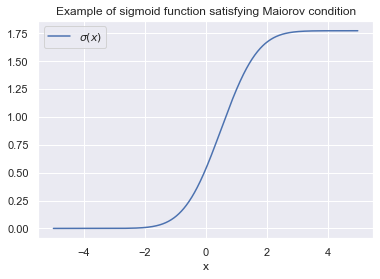
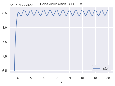
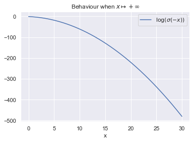
Figure 1: Activation function satisfying the Maiorov condition with $\varphi(x)=({1}/{\sqrt{2}})e^{-{x^{2}}/{2}}$

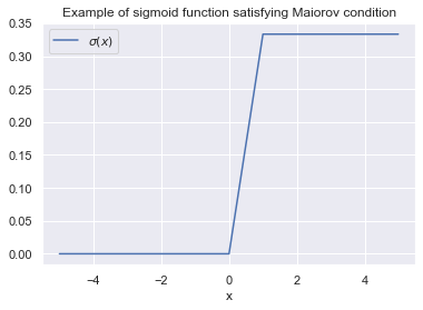
Figure 2: Sigmoid function satisfying the Maiorov condition with $\varphi(x)={(1-|x|)_{+}}/{3}$.

In Figure 1 we display the function $\sigma$ defined in Lemma 4, as well as its limit behaviour when $|x|\rightarrow+\infty$. The left plot shows that $\sigma$ looks very much like a standard sigmoid function. The middle and the right plot zoom on the limit behavior at $+\infty$ and $-\infty$, respectively. We see, in particular, that $\sigma$ is not monotone when its values get close to its upper limit, but that it is bounded everywhere and tends exponentially fast to $0$ at $-\infty$. We can also consider the case where $\varphi(x)=\frac{(1-|x|)_{+}}{3}$, for which we displayed, in Figure 2, the corresponding activation function $\sigma$. The function $\sigma$ is derived using the same methodology as for the case of Lemma 4 (see also Section A.4).

5.2 Bounds for the ReLU activation function

The literature on neural networks with ReLU activation has significantly grown these last years thanks to the computational benefits of considering piecewise linear activation functions (Yarotsky, 2017, 2018; Yarotsky and Zhevnerchuk, 2020; Gühring et al., 2020; Lu et al., 2020; Shen et al., 2019). We review below the results concerning shallow networks only, leaving aside the rich literature on approximation properties of deep networks.

For a Lipschitz function $f$, approximation error of order $O(\eta D_{1}^{-{1}/{D_{0}}})$ is obtained in (Bach, 2017). Following the seminal work (Makovoz, 1996), results for Barron spectral spaces were developed in (Klusowski and Barron, 2016a; Xu, 2020; Siegel and Xu, 2020). Let $\Omega\subset\mathbb{R}^{D_{0}}$ be a bounded domain and $s>0$. The Barron spectral space of order $s$ on $\Omega$ is

$$\mathscr{B}^{s}(\Omega):=\Big{\{}f:\Omega\mapsto\mathbb{C}:\|f\|_{\mathscr{B}^{s}(\Omega)}:=\inf_{f_{e}|\Omega=f}\int_{\mathbb{R}^{d}}\left(1+\|\bm{z}\|_{2}\right)^{s}|\mathscr{F}[f_{e}](\bm{z})|d\bm{z}<\infty\Big{\}},$$ (23)

where $f_{e}$ is an $L^{1}(\mathbb{R}^{d})$ extension of $f$. It was shown in (Klusowski and Barron, 2016a) that the approximation error over $\mathscr{B}^{2}([0,1]^{D_{0}})$ is $O(D_{1}^{-{(D_{0}+2)}/{(2D_{0})}})$. The same was proved to hold (Xu, 2020) for ReLU^k activation defined as $\sigma^{(k)}(x)=\max(0,x)^{k}$, when the target function is in $\mathscr{B}^{k+1}([0,1]^{D_{0}})$. Very recently, (Siegel and Xu, 2020) made another step forward to assess the approximation error of shallow neural networks. This result being, to the best of our knowledge, the tightest one for shallow networks with ReLU^k activations, we provide its statement in the particular case of $k=1$.

Theorem 5 ((Siegel and Xu, 2020), Theorem 3).

Let $\Omega=[0,1]^{D_{0}}$ and $s\geq{1}/{2}$. If $f\in\mathscr{B}^{s}(\Omega)$ and $D_{1}\geq 2$, then

$$\|f-f_{\bm{w}^{*}}\|_{\mathbb{L}_{2}(\Omega)}\leq C\|f\|_{\mathscr{B}^{s}(\Omega)}D_{1}^{-K}\log^{m}(D_{1}),$$ (24)

where $C$ is a constant depending on $s$ and $D_{0}$ (but not on $D_{1}$), whereas $K$ and $m$ are given by

$$K=\begin{cases}2&\text{if}\;2s\geq{3}D_{0}+4\\ \frac{1}{2}+\frac{2s-1}{2(D_{0}+1)}&\text{if}\;2s<{3}D_{0}+4\end{cases}\qquad\text{and}\qquad m=\begin{cases}0&\text{if}\;2s<3D_{0}+4\\ 1&\text{if}\;2s>3D_{0}+4\\ \frac{5}{2}&\text{if}\;2s=3D_{0}+4.\end{cases}$$ (25)

Note that in the papers summarized in this section, the values of the constants—that may depend on the input dimension and on the smoothness—are not specified. A unfortunate consequence of this is that we can not keep track of the information on the role of the input dimension in the risk bounds stated in the next section.

6 Worst-case risk bounds over smoothness classes

This section is devoted to upper bounds on the minimax risk. We present risk bounds for networks with sigmoid activation functions and prior to treating the case of ReLU activation.

6.1 Sigmoid activation functions

In this section we focus on real valued functions ($D_{2}=1$) belonging to the unit ball of the Sobolev space, $f_{\mathbf{P}}\in W_{2}^{r}([0,1]^{D_{0}},\mu)$. Using Theorem 2 and Theorem 3, we can express both the estimation and the approximation error as functions of the size $D_{1}$ of the hidden layer for an activation function that satisfies the conditions of Theorem 3. This leads to the risk bound

$$C_{\mathsf{PB}}^{-1}\mathbf{E}_{\mathbf{P}}\big{[}\|\widehat{f}_{n}-f_{\mathbf{P}}\|_{\mathbb{L}_{2}(\mu)}^{2}\big{]}\leq 2c_{1}^{2}B^{2}_{\varphi}\frac{\log^{2}(D_{1})}{D_{1}^{2r/D_{0}}}+\frac{4\beta D_{1}D_{0}}{n}\log\Big{(}3+\frac{nE}{d\beta}\Big{)},$$ (26)

where $c_{1}B_{\varphi}$ is as defined in Theorem 3, and $E$ is defined in Theorem 2. We clearly see that $D_{1}$, the width of the hidden layer, controls the extent to which finer structure can be modeled. Reducing $D_{1}$ decreases the estimation error since we have fewer parameters to estimate. But it increases the approximation error since we use a narrower class of approximators. Our goal below is to determine the value of $D_{1}$ guaranteeing the best trade-off between approximation and estimation errors.

Theorem 6 (Sigmoidal activation and Sobolev balls).

Let $\mathcal{X}=[0,1]^{D_{0}}$ and $r>0$. Let $\widehat{f}_{n}$ be an aggregate of neural networks satisfying PAC-Bayes risk bound (4). If the measure $\mu$ and the activation function $\sigma$ satisfy conditions of Theorem 3, then the choice

$$D_{1}=\Big{(}\frac{\beta D_{0}}{n}\Big{)}^{-\frac{D_{0}}{2r+D_{0}}}$$ (27)

leads to the worst-case risk bound

$$\sup_{\mathbf{P}:f_{\mathbf{P}}\in W_{2}^{r}(\mathcal{X},\mu)}\mathbf{E}_{\mathbf{P}}\big{[}\|\widehat{f}_{n}-f_{\mathbf{P}}\|_{\mathbb{L}_{2}(\mu)}^{2}\big{]} \leq g(n)\Big{(}\frac{\beta D_{0}}{n}\Big{)}^{{2r}/(2r+D_{0})},$$ (28)

where $g(n)$ is the slowly varying function

$$g(n)=2C_{\mathsf{PB}}\bigg{(}c_{1}^{2}B_{\varphi}^{2}\log^{2}(n/\beta)+2\log\Big{(}3+\frac{3nB_{2}^{2}(B_{1}^{2}M_{2}^{2}+\mu(\mathcal{X})M_{\sigma}^{2})}{d\beta}\Big{)}\bigg{)}.$$ (29)

The proof of this theorem consists in substituting $D_{1}$ in (26) by its expression (27). The obtained rate, $n^{-2r/(2r+D_{0})}$, is the classical minimax rate of estimation over $D_{0}$-variate and $r$-smooth functions. We further discuss this result and compare it to prior work in Section 6.3.

6.2 ReLU activation function

In the case of ReLU activation, we will state risk bounds two classes: the Barron spectral space and a specific Sobolev ball. Let us first assume that $f_{\mathcal{P}}\in\mathscr{B}^{s}([0,1]^{D_{0}})$ and that the conditions of Theorem 5 are satisfied. In view of Theorem 2 and Theorem 5, we have the risk bound

$$\mathbf{E}_{\mathbf{P}}\big{[}\|\widehat{f}_{n}-f_{\mathcal{P}}\|_{\mathbb{L}_{2}(\mu)}^{2}\big{]} \leq 2C_{\textsf{PB}}C^{2}D_{1}^{-2K(s,D_{0})}\log^{2m}(D_{1})+C_{\textsf{PB}}\frac{4\beta D_{1}D_{0}}{n}\log\Big{(}3+\frac{nE}{d\beta}\Big{)}$$ (30)

where $C$, $K=K(s,D_{0})$, $m$ are as in Theorem 5 and $E$ is as in Theorem 2. The bias-variance balance equation takes the form $D_{1}^{-2K}\asymp{\beta D_{1}}/{n}$ and leads to the following proposition.

Proposition 7 (ReLU activation and Barron spectral spaces).

Let $K=K(s,D_{0})$ be as in (25) and let $\widehat{f}_{n}$ be an aggregate of neural networks satisfying PAC-Bayes risk bound (4). If the conditions of Theorem 5 hold then the choice $D_{1}=\big{(}{\beta D_{0}}/{n}\big{)}^{-1/(2K+1)}$ leads to the risk bound

$$\sup_{\|f_{\mathbf{P}}\|_{\mathscr{B}^{s}([0,1]^{D_{0}})}\leq 1}\mathbf{E}_{\mathbf{P}}\big{[}\|\widehat{f}_{n}-f_{\mathbf{P}}\|_{\mathbb{L}_{2}(\mu)}^{2}\big{]} \leq\bar{g}(n)\Big{(}\frac{\beta D_{0}}{n}\Big{)}^{{2K}/(2K+1)},$$ (31)

with the slowly varying function

$$\bar{g}(n) =2C_{\mathsf{PB}}C^{2}\log^{2m}(n/\beta)+4C_{\mathsf{PB}}\log\left(3+\frac{3nB_{1}^{2}B_{2}^{2}(M_{2}^{2}+\bar{M}_{2}^{2})}{d\beta}\right)$$ (32)

and $C$ is a constant that depends on $s$ and $D_{0}$ but not on $D_{1}$.

To get a risk over Sobolev spaces, we can rely on the inclusion $W^{s+\nicefrac{{D_{0}}}{{2}}+\varepsilon,2}(\mathcal{X})\subset\mathscr{B}^{s}(\mathcal{X})$, true for arbitrarily small $\varepsilon>0$ (Xu, 2020, Lemma 2.5). This is equivalent to $W^{r,2}(\mathcal{X})\subset\mathscr{B}\/^{\bar{r}-\nicefrac{{D_{0}}}{{2}}}(\mathcal{X})$ for every $r$, $\bar{r}$ such that $D_{0}/2\leq\bar{r}<r$. Depending on the order of the Barron spectral space and the dimension of the problem, this might require a significant level of smoothness for the function $f$ we want to approximate. Keeping this constraint in mind, we proceed with the next proposition which is more easily comparable to Theorem 6.

Proposition 8 (ReLU activation and Sobolev space).

Let $r\in({D_{0}}/{2},2D_{0}+2)$ and let $\widehat{f}_{n}$ be an aggregate satisfying (4). For every $\bar{r}<r$ there is a slowly varying function $g_{\bar{r}}:\mathbb{N}\to\mathbb{R}_{+}$ such that

$$\sup_{f_{\mathbf{P}}\in W_{2}^{r}([0,1]^{D_{0}})}\mathbf{E}_{\mathbf{P}}\big{[}\|\widehat{f}_{n}-f_{\mathbf{P}}\|_{\mathbb{L}_{2}(\mu)}^{2}\big{]} \leq g_{\bar{r}}(n)n^{-\frac{2\bar{r}}{2\bar{r}+D_{0}+1}}.$$ (33)

This result is weaker than the one of Theorem 6 in three aspects. First, it has the constraint $r\in({D_{0}}/{2},2D_{0}+2)$ limiting the order of smoothness of Sobolev classes. The constraint $r<2D_{0}+2$ stems from the fact that we want $K(s,D_{0})$ to take the value $(2s+D_{0})/(2D_{0}+2)$. If $r\geq 2D_{0}+2$, the claim of the last proposition holds true if we replace $2\bar{r}/(2\bar{r}+D_{0}+1)$ by $4/5$. The second weakness is that $\bar{r}$, present in the rate of convergence, is strictly smaller than the true smoothness $r$. Finally, the denominator in the exponent has an additional term increasing the dimension $D_{0}$ by 1, leading thus to a slightly slower rate of convergence than the minimax rate over Sobolev balls. This is a direct consequence of approximation properties of ReLU neural nets in Sobolev spaces.

6.3 Related work on risk bounds for (penalized) ERM neural networks

For shallow neural networks with sigmoid activation, (Barron, 1994) showed that the risk of the suitably penalized empirical risk minimizer (ERM) is $O(n^{-1/2}\log n)$, provided that the function $f$ is very smooth ($\int\|\bm{z}\|_{1}|\mathscr{F}[f](z)|\,dz<\infty$). This was improved to $O\left(n^{-{2\bar{r}}/{(2\bar{r}+D_{0}+5)}}\right)$, $\forall\bar{r}<r$, for specific cosine activation (McCaffrey and Gallant, 1994). To our knowledge, this is the best known result for a one-hidden-layer network provided by ERM. In the case of two-hidden-layer networks with sigmoid activation, the rate $O(n^{-2r/(2r+D_{0})}\log^{3}n)$ was obtained in (Bauer and Kohler, 2019) for functions satisfying a generalized hierarchical interaction model. Our risk bound (28), of order $O(n^{-2r/(2r+D_{0})}\log n)$, matches the nonparametric minimax rate (Stone, 1982; Tsybakov, 2008), and is better than known rates for the ERM networks with one hidden layer. Roughly speaking, this shows that aggregation acts as an additional layer, so that the aggregated one-hidden-layer networks achieve the same rate as the ERM two-hidden-layer networks.

We switch now to neural networks with ReLU activation functions. For one-hidden-layer networks, (Bach, 2017) established a risk bound of order $n^{-{2}/{(D_{0}+3)}}$. On a related note, (Klusowski and Barron, 2016b) considered bounded ramp activation functions and the low dimensional setting $D_{0}\ll n$. For functions belonging to $\mathscr{B}^{2}([0,1]^{D_{0}})$, they proved that the risk of the penalized ERM is $O(n^{-{(D_{0}+4)}/{(2D_{0}+6)}})$. This result can be directly compared to ours, in the particular case $s=2$; Proposition 7 and the fact that ${2K}/{(2K+1)}={(2s+D_{0})}/{(2s+2D_{0}+1)}=(D_{0}+4)/(2D_{0}+5)$, yield a leading term of order $O\big{(}n^{-(D_{0}+4)/(2D_{0}+5)}\big{)}$. This improves the result of (Klusowski and Barron, 2016b) by a factor $O(n^{-\nicefrac{{(D_{0}+4)}}{{2(3+D_{0})(2D_{0}+5)}}})$. For instance, if $D_{0}=3$ or $D_{0}=4$, we get the improvement factors $n^{-7/132}$ and $n^{-4/91}$, respectively. This improvement vanishes when $D_{0}$ increases to infinity. For multilayer ReLU networks, (Schmidt-Hieber, 2020) established the counterpart of the risk bound of (Bauer and Kohler, 2019) for $\beta$-Hölder functions. In particular, the worst-case risk was shown to be $O(n^{-{2\beta}/{(2\beta+D_{0})}})$, see also (Suzuki, 2019) for an analogous result over Besov spaces. Hence, the minimax rate is achieved by the ERM over multilayer ReLU networks. In view of Proposition 8, this provides a bound for the ERM over multilayer networks smaller by a factor $O(n^{-{2\bar{r}}/(2\bar{r}+D_{0}+1)(2\bar{r}+D_{0})})$ then the bound for the aggregate of one-hidden-layer networks.

7 Conclusion and outlook

We have analyzed the estimation error of an aggregate of neural networks having one hidden layer and Lipschitz continuous activation function, under the condition that the aggregate satisfies the PAC-Bayes inequality. We focused our attention on Gaussian priors and obtained risk bounds in which the dependence on all the involved parameters is explicit. All these bounds on the estimation error come with explicit constants. We then combined our bounds on the estimation error with bounds on approximation error available in the literature. This allowed us to prove that aggregation of one-layer neural networks achieves the minimax risk over conventional smoothness classes. On the down side, since the constants in the bounds on the approximation error available in the literature are not explicit, the same is true for risk bounds of the present work. Therefore, it would be highly relevant to refine the existing approximation bounds to make appear all the constants.

The results of the present work can be extended in different directions. First, it would be interesting to consider the problem of aggregation of deep neural networks in order to understand possible benefits of increasing the depth. Second, it might be relevant to analyze the case of a prior with heavier tails, such as the Laplace prior or the Student prior, with a hope to cover the case of high dimension $D_{0}>n$ under some kind of sparsity assumption. Finally, another avenue of future research is to explore the computational benefits of considering aggregated neural networks in conjunction with the Langevin-type algorithms.

Appendix A Proofs

As a preliminary remark let us note that, as a mixing measure, we expect the distribution $p$ to aggregate the predictors $f_{\bm{w}}$ so that the resulting estimator is almost as good as the best predictors in $\mathcal{F}_{\mathsf{W}}$. A direct consequence of it is that “a good choice” of $p$ should be centered in $\bar{\bm{w}}$. This is an heuristic way to choose the mean, and all along the appendix we will fix the distribution of $p$ as

$$p=p_{1}\otimes p_{2}\sim\mathcal{N}(\bar{\bm{w}}_{1},\tau_{1}^{2}\mathbf{I}_{D_{1}D_{0}})\otimes\mathcal{N}(\bar{\bm{w}}_{2},\tau_{2}^{2}\mathbf{I}_{D_{1}D_{2}}),\qquad\tau_{1},\tau_{2}>0$$ (34)

where $\bar{\bm{w}}\in\text{argmin}_{\bm{w}\in\mathsf{W}}\|f_{\bm{w}}-f_{\mathbf{P}}\|_{\mathbb{L}_{2}(\mu)}$. The additional condition (34) is the starting point of our choice for $p$, it is now left to set values for the variance $(\tau_{1}^{2},\tau_{2}^{2})$.

A.1 Some useful lemmas

In what follows, when appropriate, we will write $f_{\bm{w}_{1},\bm{w}_{2}}$ instead of $f_{\bm{w}}$.

Lemma 9.

If the probability distribution $p$ is such that $p(d\bm{w})=p_{1}(d\bm{w}_{1})p_{2}(d\bm{w}_{2})$ with

$$\int_{\mathsf{W}_{2}}\bm{w}_{2}p_{2}(d\bm{w}_{2})=\bar{\bm{w}}_{2}$$ (35)

then

$$\int_{\mathsf{W}}\|f_{\bm{w}}-f_{\bar{\bm{w}}}\|_{\mathbb{L}_{2}(\mu)}^{2}\,p(d\bm{w})=\int_{\mathsf{W}}\|f_{\bm{w}}-f_{\bm{w}_{1},\bar{\bm{w}}_{2}}\|_{\mathbb{L}_{2}(\mu)}^{2}\,p(d\bm{w})+\int_{\mathsf{W}_{1}}\|f_{\bm{w}_{1},\bar{\bm{w}}_{2}}-f_{\bar{\bm{w}}}\|_{\mathbb{L}_{2}}^{2}\,p_{1}(d\bm{w}_{1}).$$ (36)

Proof.

Simple algebra yields

$$\int_{\mathsf{W}}\big{(}f_{\bm{w}}-f_{\bar{\bm{w}}}\big{)}^{2}(\bm{x})\,p(d\bm{w}) =\int_{\mathsf{W}}(f_{\bm{w}}-f_{\bm{w}_{1},\bar{\bm{w}}_{2}}+f_{\bm{w}_{1},\bar{\bm{w}}_{2}}-f_{\bar{\bm{w}}})^{2}(\bm{x})\,p(d\bm{w})$$ (37)

$$=\int_{\mathsf{W}}(f_{\bm{w}}-f_{\bm{w}_{1},\bar{\bm{w}}_{2}})^{2}(\bm{x})\,p(d\bm{w})+\int_{\mathsf{W}}(f_{\bm{w}_{1},\bar{\bm{w}}_{2}}-f_{\bar{\bm{w}}})^{2}(\bm{x})\,p(d\bm{w})$$ (38)

$$\qquad+2\underbrace{\int_{\mathsf{W}}(f_{\bm{w}_{1},\bm{w}_{2}}-f_{\bm{w}_{1},\bar{\bm{w}}_{2}})(\bm{x})(f_{\bm{w}_{1},\bar{\bm{w}}_{2}}-f_{\bar{\bm{w}}_{1},\bar{\bm{w}}_{2}})(\bm{x})\,p(d\bm{w})}_{\triangleq A}.$$ (39)

To complete the proof it suffices to integrate the previous equality with respect to $\mu(d\bm{x})$ in virtue of Fubini-Tonelli theorem and to check that $A=0$. The latter property follows from the fact that $p$ is a product measure and, for all $\bm{w}_{1}\in\mathsf{W}_{1}$,

$$\int_{\mathsf{W}_{2}}(f_{\bm{w}_{1},\bm{w}_{2}}-f_{\bm{w}_{1},\bar{\bm{w}}_{2}})(\bm{x})\,p_{2}(d\bm{w}_{2})=\int_{\mathsf{W}_{2}}(\bm{w}_{2}-\bar{\bm{w}}_{2})^{\top}\bar{\sigma}(\bm{w}_{1}^{\top}\bm{x})\,p_{2}(d\bm{w}_{2})=0.$$ (40)

This yields the claim of the lemma. ∎

In this section and the next one, let us define the two quantities:

$$G_{1}(\bm{w}) =\|f_{\bm{w}}-f_{\bm{w}_{1},\bar{\bm{w}}_{2}}\|_{\mathbb{L}_{2}(\mu)}^{2},\qquad\text{and}\qquad G_{2}(\bm{w}_{1})=\|f_{\bm{w}_{1},\bar{\bm{w}}_{2}}-f_{\bar{\bm{w}}}\|_{\mathbb{L}_{2}(\mu)}^{2}.$$ (41)

Lemma 10.

If Assumptions ($\sigma$-L) and $M_{2}<\infty$ are satisfied, and $p$ is chosen as in (34), then

$$\int_{\mathsf{W}_{1}}G_{2}(\bm{w}_{1})\,p_{1}(d\bm{w}_{1}) \leq D_{0}\big{(}M_{2}\tau_{1}\|\bar{\bm{w}}_{2}\|_{1,2}\big{)}^{2}\leq C_{1}D_{0}D_{1}\tau_{1}^{2}$$ (42)

with $C_{1}=(M_{2}\|\bar{\bm{w}}_{2}\|_{\mathsf{F}})^{2}$.

Proof of Lemma 10.

We first use the fact that $\sigma$ is 1-Lipschitz. On the one hand, in conjunction with the Fubini-Tonelli theorem, this yields

$$\int_{\mathsf{W}_{1}}G_{2}(\bm{w}_{1})\,p_{1}(d\bm{w}_{1}) =\int_{\mathcal{X}}\int_{\mathsf{W}}\left\|\bar{\bm{w}}_{2}^{\top}\left\{\bar{\sigma}(\bm{w}_{1}^{\top}\bm{x})-\bar{\sigma}(\bar{\bm{w}}_{1}^{\top}\bm{x})\right\}\right\|_{2}^{2}p(d\bm{w})\mu(d\bm{x})$$ (43)

$$\leq\int_{\mathcal{X}}\int_{\mathsf{W}}\sum_{j=1}^{D_{2}}\left(\sum_{i=1}^{D_{1}}|\bar{\bm{w}}_{2,ij}||(\bm{w}_{1}-\bar{\bm{w}}_{1})_{i}^{\top}\bm{x}|\right)^{2}p(d\bm{w})\mu(d\bm{x})$$ (44)

$$\leq\int_{\mathcal{X}}\sum_{j=1}^{D_{2}}\left(\sum_{i=1}^{D_{1}}|\bar{\bm{w}}_{2,ij}|\bigg{\{}\int_{\mathsf{W}}|(\bm{w}_{1}-\bar{\bm{w}}_{1})_{i}^{\top}\bm{x}|^{2}p(d\bm{w})\bigg{\}}^{1/2}\right)^{2}\mu(d\bm{x})$$ (45)

$$=D_{0}M_{2}^{2}\tau_{1}^{2}\sum_{j=1}^{D_{2}}\left(\sum_{i=1}^{D_{1}}|\bar{\bm{w}}_{2,ij}|\right)^{2}\leq D_{0}M_{2}^{2}\tau_{1}^{2}D_{1}\|\bar{\bm{w}}_{2}\|_{\mathsf{F}}^{2}$$ (46)

and the claim of the lemma follows. ∎

In view of Lemma 9 and Lemma 10, we have

$$\int_{\mathsf{W}}\|f_{\bm{w}}-f_{\bar{\bm{w}}}\|_{\mathbb{L}_{2}(\mu)}^{2}\,p(d\bm{w})=\int_{\mathsf{W}}G_{1}(\bm{w})\,p(d\bm{w})+\int_{\mathsf{W}}G_{2}(\bm{w}_{1})\,p_{1}(d\bm{w}_{1}).$$ (47)

and

$$\int_{\mathsf{W}}G_{2}(\bm{w}_{1})\,p(d\bm{w}) \leq D_{1}(M_{2}\|\bar{\bm{w}}_{2}\|_{\mathsf{F}})^{2}\tau^{2}_{1}.$$ (48)

We now state two distinct lemmas to bound the quantity $\int_{\mathsf{W}}G_{1}(\bm{w})\,p(d\bm{w})$. Lemma 11 account for bounded activation functions whereas Lemma 12 focuses on unbounded ones.

Lemma 11.

Under ($\sigma$-B) and $M_{2}<\infty$, if $p$ is given by (34), we have

$$\int_{\mathsf{W}}G_{1}(\bm{w})\,p(d\bm{w}) \leq(M_{\sigma}\tau_{2})^{2}\mu(\mathcal{X})D_{1}D_{2}.$$ (49)

Proof of Lemma 11.

Using Fubini-Tonelli theorem, we get

$$\int_{\mathsf{W}}G_{1}(\bm{w})\,p(d\bm{w}) =\int_{\mathcal{X}}\int_{\mathsf{W}_{1}}\underbrace{\int_{\mathsf{W}_{2}}\Big{\|}(\bm{w}_{2}-\bar{\bm{w}}_{2})^{\top}\bar{\sigma}(\bm{w}_{1}^{\top}\bm{x})\Big{\|}_{\mathbb{L}_{2}(\mu)}^{2}\,p_{2}(d\bm{w}_{2})}_{:=I(\bm{x},\bm{w}_{1})}p_{1}(d\bm{w}_{1})\,\mu(d\bm{x}).$$ (50)

For the inner integral, simple algebra yields

$$I(\bm{x},\bm{w}_{1}) =\int_{\mathsf{W}}\bar{\sigma}(\bm{w}_{1}^{\top}\bm{x})^{\top}(\bm{w}_{2}-\bar{\bm{w}}_{2})(\bm{w}_{2}-\bar{\bm{w}}_{2})^{\top}\bar{\sigma}(\bm{w}_{1}^{\top}\bm{x})\,p(d\bm{w})$$ (51)

$$=\bar{\sigma}(\bm{w}_{1}^{\top}\bm{x})^{\top}\bigg{\{}\int_{\mathsf{W}_{2}}(\bm{w}_{2}-\bar{\bm{w}}_{2})(\bm{w}_{2}-\bar{\bm{w}}_{2})^{\top}\,p_{2}(d\bm{w}_{2})\bigg{\}}\bar{\sigma}(\bm{w}_{1}^{\top}\bm{x})$$ (52)

$$=\tau_{2}^{2}D_{2}\|\bar{\sigma}(\bm{w}_{1}^{\top}\bm{x})\|_{2}^{2}.$$ (53)

Therefore,

$$\int_{\mathcal{X}}\int_{\mathsf{W}_{1}}I(\bm{x},\bm{w}_{1})\,p_{1}(d\bm{w}_{1})\,\mu(d\bm{x})\leq M_{\sigma}^{2}\mu(\mathcal{X})\tau^{2}_{2}D_{1}D_{2}.$$ (54)

This completes the proof of the lemma. ∎

Lemma 12.

Let $\bar{M}_{2}=\|\int_{\mathcal{X}}\bm{x}\bm{x}^{\top}\mu(d\bm{x})\|_{\mathsf{sp}}$ be the spectral norm of the “covariance” matrix of the design. Under ($\sigma$-L), if $p$ is given by (34) and $\sigma(0)=0$, we have

$$\int_{\mathsf{W}}G_{1}(\bm{w})\,p(d\bm{w}) \leq M_{2}^{2}D_{0}D_{1}D_{2}\tau_{1}^{2}\tau_{2}^{2}+\bar{M}_{2}^{2}D_{2}\|\bar{\bm{w}}_{1}\|_{\mathsf{F}}^{2}\tau_{2}^{2}.$$ (55)

Proof of Lemma 12.

Using (53), we get

$$\int_{\mathsf{W}}G_{1}( \bm{w})\,p(d\bm{w})=\tau_{2}^{2}D_{2}\int_{\mathcal{X}}\int_{\mathsf{W}_{1}}\|\bar{\sigma}(\bm{w}_{1}^{\top}\bm{x})\|_{2}^{2}\,p_{1}(d\bm{w}_{1})\,\mu(d\bm{x})$$ (56)

$$\leq\tau_{2}^{2}D_{2}\int_{\mathcal{X}}\int_{\mathsf{W}_{1}}\|\bm{w}_{1}^{\top}\bm{x}\|_{2}^{2}\,p_{1}(d\bm{w}_{1})\,\mu(d\bm{x})$$ (57)

$$=\tau_{2}^{2}D_{2}\int_{\mathcal{X}}\int_{\mathsf{W}_{1}}\|(\bm{w}_{1}-\bar{\bm{w}}_{1})^{\top}\bm{x}\|_{2}^{2}\,p_{1}(d\bm{w}_{1})\,\mu(d\bm{x})+\tau_{2}^{2}D_{2}\int_{\mathcal{X}}\|(\bar{\bm{w}}_{1})^{\top}\bm{x}\|_{2}^{2}\,\mu(d\bm{x})$$ (58)

$$=M_{2}^{2}D_{0}D_{1}D_{2}\tau_{1}^{2}\tau_{2}^{2}+\bar{M}_{2}^{2}D_{2}\|\bar{\bm{w}}_{1}\|_{\mathsf{F}}^{2}\tau_{2}^{2}.$$ (59)

This completes the proof of the lemma. ∎

Lemma 13.

Under ($\sigma$-L) and $M_{2}<\infty$, if $p$ is given by (34), then

$$\int_{\mathsf{W}}\|f_{\bm{w}}-f_{\bar{\bm{w}}}\|_{\mathbb{L}_{2}(\mu)}^{2}\,p(d\bm{w})\leq M^{2}_{2}\|\bar{\bm{w}}_{2}\|_{\mathsf{F}}^{2}D_{0}D_{1}\tau^{2}_{1}+\bar{M}_{2}^{2}D_{2}\|\bar{\bm{w}}_{1}\|_{\mathsf{F}}^{2}\tau_{2}^{2}+M_{2}^{2}D_{0}D_{1}D_{2}\tau_{1}^{2}\tau_{2}^{2}.$$ (60)

If, in addition, ($\sigma$-B) is satisfied, then

$$\int_{\mathsf{W}}\|f_{\bm{w}}-f_{\bar{\bm{w}}}\|_{\mathbb{L}_{2}(\mu)}^{2}\,p(d\bm{w})\leq M^{2}_{2}\|\bar{\bm{w}}_{2}\|_{\mathsf{F}}^{2}D_{0}D_{1}\tau^{2}_{1}+\mu(\mathcal{X})M^{2}_{\sigma}D_{1}D_{2}\tau^{2}_{2}.$$ (61)

Proof.

In Lemma 9 we have checked that

$$\int_{\mathsf{W}}\|f_{\bm{w}}-f_{\bar{\bm{w}}}\|_{\mathbb{L}_{2}(\mu)}^{2}\,p(d\bm{w})=\int_{\mathsf{W}}G_{1}(\bm{w})\,p(d\bm{w})+\int_{\mathsf{W}}G_{2}(\bm{w}_{1})\,p_{1}(d\bm{w}_{1}).$$ (62)

Lemma 11 and Lemma 10 take care of both integrals in the right hand side of the equality for bounded activation functions and we directly get (61). Similarly, Lemma 12 and Lemma 10 can be applied for unbounded activation functions, leading to (60). ∎

A.2 Proof of Proposition 1

Recall that the goal is to find an upper bound for the remainder term

$$\textup{Rem}_{n}(\bar{\bm{w}})\triangleq\inf_{p\in\mathcal{P}_{1}(\mathcal{F}_{\mathsf{W}})}\bigg{\{}\int_{\mathsf{W}}\|f_{\bm{w}}-f_{\bar{\bm{w}}}\|_{\mathbb{L}_{2}(\mu)}^{2}\,p(d\bm{w})+\frac{\beta}{n}\,D_{\textsf{KL}}(p||\pi)\bigg{\}}.$$ (63)

We start this proof by considering the case where Assumptions ($\sigma$-L), ($\sigma$-B) and ($\mathcal{N}$) are satisfied. We choose as $p$ the product of two spherical Gaussian distributions with variances $\tau_{1}^{2}$ and $\tau_{2}^{2}$, as specified in (34). In this case, the Kullback-Leibler divergence $D_{\textsf{KL}}(p||\pi)$ is given by

$$D_{\textsf{KL}}(p||\pi)=\frac{1}{2}\sum_{\ell=1}^{2}\bigg{\{}\frac{\|\bar{\bm{w}}_{\ell}\|_{\mathsf{F}}^{2}}{\rho_{\ell}^{2}}+D_{\ell-1}D_{\ell}\bigg{[}\left(\frac{\tau_{\ell}}{\rho_{\ell}}\right)^{2}-1-\log\left(\frac{\tau^{2}_{\ell}}{\rho^{2}_{\ell}}\right)\bigg{]}\bigg{\}}.$$ (64)

It is now left to find good values for $\tau^{2}_{1}$ and $\tau_{2}^{2}$. Combining with the result (61) of Lemma 13, we get the inequality

$$\textup{Rem}_{n}(\bar{\bm{w}})\leq\frac{\beta\|\bar{\bm{w}}_{1}\|_{\mathsf{F}}^{2}}{2n\rho_{1}^{2}}+\frac{\beta\|\bar{\bm{w}}_{2}\|_{\mathsf{F}}^{2}}{2n\rho_{2}^{2}}+\frac{\beta}{2n}\sum_{\ell=1}^{2}D_{\ell-1}D_{\ell}\bigg{\{}C_{\ell}\left(\frac{\tau_{\ell}}{\rho_{\ell}}\right)^{2}-1-\log\left(\frac{\tau^{2}_{\ell}}{\rho^{2}_{\ell}}\right)\bigg{\}}$$ (65)

where

$$C_{1}=\frac{2nM_{2}^{2}\|\bar{\bm{w}}_{2}\|_{\mathsf{F}}^{2}\rho_{1}^{2}}{\beta}+1,\quad C_{2}=\frac{2n\mu(\mathcal{X})M_{\sigma}^{2}\rho_{2}^{2}}{\beta}+1.$$ (66)

One can easily check that the minimum of the function $u\mapsto Cu-1-\log u$ is attained at $u_{\min}=1/C$ and the value at this point is $\log C$. This implies that

$$\textup{Rem}_{n}(\bar{\bm{w}}) \leq\frac{\beta\|\bar{\bm{w}}_{1}\|_{\mathsf{F}}^{2}}{2n\rho_{1}^{2}}+\frac{\beta\|\bar{\bm{w}}_{2}\|_{\mathsf{F}}^{2}}{2n\rho_{2}^{2}}+\frac{\beta}{2n}\sum_{\ell=1}^{2}D_{\ell-1}D_{\ell}\log C_{\ell}$$ (67)

$$\stackrel{{\scriptstyle(1)}}{{\leq}}\frac{\beta\|\bar{\bm{w}}_{1}\|_{\mathsf{F}}^{2}}{2n\rho_{1}^{2}}+\frac{\beta\|\bar{\bm{w}}_{2}\|_{\mathsf{F}}^{2}}{2n\rho_{2}^{2}}+\frac{\beta d}{2n}\log\left(\frac{D_{0}D_{1}C_{1}+D_{1}D_{2}C_{2}}{d}\right)$$ (68)

$$\leq\frac{\beta\|\bar{\bm{w}}_{1}\|_{\mathsf{F}}^{2}}{2n\rho_{1}^{2}}+\frac{\beta\|\bar{\bm{w}}_{2}\|_{\mathsf{F}}^{2}}{2n\rho_{2}^{2}}+\frac{\beta d}{2n}\log\bigg{(}1+\frac{2n(D_{0}D_{1}M_{2}^{2}\|\bar{\bm{w}}_{2}\|_{\mathsf{F}}^{2}\rho_{1}^{2}+D_{1}D_{2}\mu(\mathcal{X})M_{\sigma}^{2}\rho_{2}^{2})}{\beta d}\bigg{)},$$ (69)

where in (1) we have used the concavity of the function $u\mapsto\log u$. This completes the proof of the first claim of Proposition 1.

In the case where ($\sigma$-B) is not fulfilled, but instead $\sigma(0)=0$, we repeat the same scheme of proof as above by using (60) instead of (61). This leads to

$$\textup{Rem}_{n}(\bar{\bm{w}}) \leq\frac{\beta d}{2n}\bigg{\{}C^{\prime}_{1}\left(\frac{\tau_{1}}{\rho_{1}}\right)^{2}+C_{2}^{\prime}\left(\frac{\tau_{2}}{\rho_{2}}\right)^{2}+C_{3}^{\prime}\left(\frac{\tau_{1}}{\rho_{1}}\right)^{2}\left(\frac{\tau_{2}}{\rho_{2}}\right)^{2}-2-\log\left(\frac{\tau^{2}_{1}\tau^{2}_{2}}{\rho^{2}_{1}\rho^{2}_{2}}\right)\bigg{\}}$$ (70)

$$\qquad+\frac{\beta\|\bar{\bm{w}}_{1}\|_{\mathsf{F}}^{2}}{2n\rho_{1}^{2}}+\frac{\beta\|\bar{\bm{w}}_{2}\|_{\mathsf{F}}^{2}}{2n\rho_{2}^{2}}.$$ (71)

where

$$C^{\prime}_{1}=\frac{2nD_{0}M_{2}^{2}\|\bar{\bm{w}}_{2}\|_{\mathsf{F}}^{2}\rho_{1}^{2}}{\beta(D_{0}+D_{2})}+1,\quad C^{\prime}_{2}=\frac{2n\bar{M}_{2}^{2}\|\bar{\bm{w}}_{1}\|^{2}_{\mathsf{F}}D_{2}\rho_{2}^{2}}{\beta(D_{0}+D_{2})D_{1}}+1,\quad C_{3}^{\prime}=\frac{2nM_{2}^{2}\rho_{1}^{2}\rho_{2}^{2}D_{0}D_{2}}{\beta(D_{0}+D_{2})}.$$ (72)

We choose $\tau_{1}$ and $\tau_{2}$ so that

$$\bigg{(}\frac{\tau_{1}}{\rho_{1}}\bigg{)}^{2}=\frac{1}{C_{1}^{\prime}+C_{3}^{\prime}(\tau_{2}/\rho_{2})^{2}},\qquad\bigg{(}\frac{\tau_{2}}{\rho_{2}}\bigg{)}^{2}=1/C_{2}^{\prime}.$$ (73)

With this choice of $\tau_{1}$ and $\tau_{2}$ in (71) and simple algebra, we get

$$\textup{Rem}_{n}(\bar{\bm{w}}) \leq\frac{\beta d}{2n}\,\log\big{(}C_{1}^{\prime}C_{2}^{\prime}+C_{3}^{\prime}\big{)}+\frac{\beta\|\bar{\bm{w}}_{1}\|_{\mathsf{F}}^{2}}{2n\rho_{1}^{2}}+\frac{\beta\|\bar{\bm{w}}_{2}\|_{\mathsf{F}}^{2}}{2n\rho_{2}^{2}}.$$ (74)

To complete the proof, we use the following inequalities

$$\ln(C_{1}^{\prime}C_{2}^{\prime}+C_{3}^{\prime}) \leq\log\big{(}C_{1}^{\prime}(C_{2}^{\prime}+C_{3}^{\prime})\big{)}$$ (75)

$$=\log C_{1}^{\prime}+\log(C_{2}^{\prime}+C_{3}^{\prime})$$ (76)

$$\leq 2\ln((C_{1}^{\prime}+C_{2}^{\prime}+C_{3}^{\prime})/2),$$ (77)

where the first inequality follows from the fact that $C_{2}^{\prime}\geq 1$ whereas the last inequality is a consequence of the concavity of the logarithm.

Remark 14.

The distribution $p$ is centered on the oracle choice $\bar{\bm{w}}$ for the weights of the neural network and we observe that the optimized variances $(\tau_{1}^{2},\tau_{2}^{2})$ in the proof of Proposition 1 are of the form $\tau^{2}_{l}={\rho^{2}_{\ell}}/{(1+c_{\ell}n\rho^{2}_{\ell})}$, $\ell=1,2,$ for some positive constants $c_{1},c_{2}$. These values of $\tau_{\ell}$ arbitrate between the prior beliefs and the information brought by data. Indeed, $(1)$ when no training data is available the uncertainty around $\bar{\bm{w}}$ corresponds to the prior uncertainty $(\rho^{2}_{1},\rho_{2}^{2})$, $(2)$ when the amount of observations $n$ is unlimited and goes to infinity the uncertainty around the oracle value converges to $0$ and $p$ becomes close to the Dirac mass in $\bar{\bm{w}}$.

A.3 Proof of Theorem 2

The main idea is to choose $\rho_{1}$ and $\rho_{2}$ minimizing the upper bound of the worst-case value of the remainder term

$$\sup_{\bar{\bm{w}}:\|\bar{\bm{w}}_{\ell}\|_{\mathsf{F}}\leq B_{\ell}}\text{Rem}_{n}(\bar{\bm{w}})$$ (78)

furnished by Proposition 1. Instead of using the exact minimizer, we use a surrogate obtained by simplifying expressions of $\rho_{1}$ and $\rho_{2}$. This is done by the following result.

Corollary 15.

Let Assumptions ($\sigma$-L) and ($\mathcal{N}$) be satisfied, set $B_{\ell}=\rho_{\ell}\sqrt{2D_{\ell-1}D_{\ell}}$ for $\ell=1,2$.

• If ($\sigma$-B) holds true, then

  $$\sup_{\bar{\bm{w}}:\|\bar{\bm{w}}_{\ell}\|_{\mathsf{F}}\leq B_{\ell}}\textup{Rem}_{n}(\bar{\bm{w}})\leq\frac{\beta d}{n}\log\bigg{(}3+\frac{3nB_{2}^{2}(B_{1}^{2}M_{2}^{2}+\mu(\mathcal{X})M_{\sigma}^{2})}{d\beta}\bigg{)}.$$ (79)

• If the activation function is unbounded but vanishes at the origin, then

  $$\sup_{\bar{\bm{w}}:\|\bar{\bm{w}}_{\ell}\|_{\mathsf{F}}\leq B_{\ell}}\textup{Rem}_{n}(\bar{\bm{w}})\leq\frac{\beta d}{n}\log\left(3+\frac{3nB_{1}^{2}B_{2}^{2}(M_{2}^{2}+\bar{M}_{2}^{2}/D_{1})}{d\beta}\right).$$ (80)

The rest of this section is devoted to the proof of this claim, which implies the claim of Theorem 2. In view of (67), we have

$$\textup{Rem}_{n}(\bar{\bm{w}}) \leq\frac{\beta\|\bar{\bm{w}}_{1}\|_{\mathsf{F}}^{2}}{2n\rho_{1}^{2}}+\frac{\beta\|\bar{\bm{w}}_{2}\|_{\mathsf{F}}^{2}}{2n\rho_{2}^{2}}+\frac{\beta}{2n}\sum_{\ell=1}^{2}D_{\ell-1}D_{\ell}\log(1+F_{\ell}\rho_{\ell}^{2})$$ (81)

with

$$F_{1}=\frac{2nM_{2}^{2}\|\bar{\bm{w}}_{2}\|_{\mathsf{F}}^{2}}{\beta}\qquad\text{and}\qquad F_{2}=\frac{2n\mu(\mathcal{X})M_{\sigma}^{2}}{\beta}.$$ (82)

Taking the maximum over all $\bar{\bm{w}}$ such that the Frobenius norms of $\bar{\bm{w}}_{1}$ and $\bar{\bm{w}}_{2}$ are bounded by $B_{1}$ and $B_{2}$, we get

$$\sup_{\|\bar{\bm{w}}_{1}\|_{\mathsf{F}}\leq B_{1}}\sup_{\|\bar{\bm{w}}_{2}\|_{\mathsf{F}}\leq B_{2}}\textup{Rem}_{n}(\bar{\bm{w}}) \leq\frac{\beta B_{1}^{2}}{2n\rho_{1}^{2}}+\frac{\beta B_{2}^{2}}{2n\rho_{2}^{2}}+\frac{\beta}{2n}\sum_{\ell=1}^{2}D_{\ell-1}D_{\ell}\log(1+\bar{F}_{\ell}\rho_{\ell}^{2})$$ (83)

with

$$\bar{F}_{1}=\frac{2nM_{2}^{2}B_{2}^{2}}{\beta}\qquad\text{and}\qquad\bar{F}_{2}=\frac{2n\mu(\mathcal{X})M_{\sigma}^{2}}{\beta}.$$ (84)

The first order necessary condition for optimizing the right hand side with respect to $\rho_{1}^{2}$ and $\rho_{2}^{2}$ reads as

$$-\frac{B_{\ell}^{2}}{\rho_{\ell}^{4}}+\frac{D_{\ell-1}D_{\ell}\bar{F}_{\ell}}{1+\bar{F}_{\ell}\rho_{\ell}^{2}}=0\quad\Longleftrightarrow\quad\rho_{\ell}^{4}-\frac{B_{\ell}^{2}}{D_{\ell-1}D_{\ell}}\,\rho_{\ell}^{2}-\frac{B_{\ell}^{2}}{D_{\ell-1}D_{\ell}\bar{F}_{\ell}}=0.$$ (85)

This second-order equation has only one positive root given by

$$\rho_{\ell}^{2} =\frac{B_{\ell}^{2}}{2D_{\ell-1}D_{\ell}}+\bigg{(}\frac{B_{\ell}^{4}}{4D_{\ell-1}^{2}D_{\ell}^{2}}+\frac{B_{\ell}^{2}}{D_{\ell-1}D_{\ell}\bar{F}_{\ell}}\bigg{)}^{1/2}$$ (86)

$$=\frac{B_{\ell}^{2}}{2D_{\ell-1}D_{\ell}}\bigg{\{}1+\bigg{(}1+\frac{4D_{\ell-1}D_{\ell}}{B_{\ell}^{2}\bar{F}_{\ell}}\bigg{)}^{1/2}\bigg{\}}.$$ (87)

We simplify computations by choosing

$$\rho_{\ell}^{2} =\frac{B_{\ell}^{2}}{2D_{\ell-1}D_{\ell}}.$$ (88)

Replacing these values of $\rho_{\ell}^{2}$ in (83), we get

$$\sup_{\|\bar{\bm{w}}_{\ell}\|_{\mathsf{F}}\leq B_{\ell}}\textup{Rem}_{n}(\bar{\bm{w}}) \leq\frac{\beta}{n}\sum_{\ell=1}^{2}D_{\ell-1}D_{\ell}\bigg{\{}1+\frac{1}{2}\log\bigg{(}1+\frac{B_{\ell}^{2}\bar{F}_{\ell}}{2D_{\ell-1}D_{\ell}}\bigg{)}\bigg{\}}$$ (89)

$$\leq\frac{\beta d}{n}\sum_{\ell=1}^{2}\bigg{\{}1+\frac{1}{2}\log\bigg{(}1+\frac{B_{1}^{2}\bar{F}_{1}+B_{2}^{2}\bar{F}_{2}}{2d}\bigg{)}\bigg{\}},$$ (90)

where the last inequality follows from the concavity of the logarithm. Replacing $\bar{F}_{1}$ and $\bar{F}_{2}$ with their respective expressions, we get the inequality

$$\sup_{\|\bar{\bm{w}}_{\ell}\|_{\mathsf{F}}\leq B_{\ell}}\textup{Rem}_{n}(\bar{\bm{w}}) \leq\frac{\beta d}{n}\Bigg{(}1+\frac{1}{2}\log\bigg{(}1+\frac{nB_{2}^{2}(B_{1}^{2}M_{2}^{2}+\mu(\mathcal{X})M_{\sigma}^{2})}{d\beta}\bigg{)}\Bigg{)}$$ (91)

$$\leq\frac{\beta d}{n}\log\bigg{(}3+\frac{3nB_{2}^{2}(B_{1}^{2}M_{2}^{2}+\mu(\mathcal{X})M_{\sigma}^{2})}{d\beta}\bigg{)},$$ (92)

which coincides with the first claim of the corollary.

The second claim of the proposition is obtained by replacing $\rho_{\ell}$’s by their respective expressions in the second claim of Proposition 1.

A.4 Proof of Proposition 4

Since

$$\sigma(x)=\sum_{j=1}^{\infty}\varphi(x-j).$$ (93)

we have

$$\sigma(x+1)-\sigma(x) =\sum_{j=1}^{\infty}\varphi(x+1-j)-\sum_{j=1}^{\infty}\varphi(x-j)$$ (94)

$$=\sum_{j=0}^{\infty}\varphi(x-j)-\sum_{j=1}^{\infty}\varphi(x-j)$$ (95)

$$=\varphi(x).$$ (96)

Now, recall that we use the function $\varphi(x)=\frac{1}{\sqrt{2}}e^{-{x^{2}}/{2}}$. It is clear, that the series

$$\sum_{j=1}^{\infty}|\varphi^{\prime}(j-x)|$$ (97)

converges uniformly on any bounded interval. This implies that $\sigma$ is differentiable and

$$\sigma^{\prime}(x)=\sum_{j=1}^{\infty}\frac{(j-x)}{\sqrt{2}}e^{-{(x-j)^{2}}/{2}}.$$ (98)

Let us denote by $[x]$ the integer part of $x$ and by $\{x\}=x-[x]$ the fractional part of $x$. Recall also that the function $u\mapsto e^{-u^{2}/2}$ is increasing on $(-\infty,0]$ and decreasing on $[0,+\infty)$. Therefore, we have

$$\sigma(x) =\frac{1}{\sqrt{2}}\sum_{j=1}^{[x]}e^{-{(x-j)^{2}}/{2}}+\frac{1}{\sqrt{2}}\sum_{j=[x]+1}^{\infty}e^{-{(x-j)^{2}}/{2}}$$ (99)

$$\leq\frac{1}{\sqrt{2}}\sum_{j=1}^{[x]-1}\int_{x-j-1}^{x-j}e^{-u^{2}/{2}}\,du+\frac{e^{-\{x\}^{2}/2}+e^{-(1-\{x\})^{2}/2}}{\sqrt{2}}+\frac{1}{\sqrt{2}}\sum_{j=[x]+2}^{\infty}\int_{j-x-1}^{j-x}e^{-u^{2}/{2}}\,du$$ (100)

$$\leq\frac{1}{\sqrt{2}}\int_{\{x\}}^{x-1}e^{-u^{2}/{2}}\,du+\frac{e^{-\{x\}^{2}/2}+e^{-(1-\{x\})^{2}/2}}{\sqrt{2}}+\frac{1}{\sqrt{2}}\int_{-\infty}^{\{x\}-1}e^{-u^{2}/{2}}\,du$$ (101)

$$\leq\frac{1}{\sqrt{2}}\int_{-\infty}^{+\infty}e^{-u^{2}/{2}}\,du+\frac{1}{\sqrt{2}}=\sqrt{\pi}+\frac{1}{\sqrt{2}}.$$ (102)

For $x>0$, using similar arguments and the fact that the function $u\mapsto ue^{-u^{2}/2}$ is decreasing on $[1,\infty)$, we get

$$\sqrt{2}\sigma^{\prime}(x) =-\sum_{j=1}^{[x]}(x-j)e^{-{(x-j)^{2}}/{2}}+\sum_{j=[x]+1}^{\infty}(j-x)e^{-{(j-x)^{2}}/{2}}$$ (103)

$$\leq(1-\{x\})e^{-(1-\{x\})^{2}/2}+\sum_{j=[x]+2}^{\infty}\int_{j-x-1}^{j-x}ue^{-u^{2}/{2}}\,du$$ (104)

$$\leq(1-\{x\})e^{-(1-\{x\})^{2}/2}+\int_{1-\{x\}}^{\infty}ue^{-u^{2}/{2}}\,du$$ (105)

$$=(2-\{x\})e^{-(1-\{x\})^{2}/2}\leq\sqrt{2}.$$ (106)

In the same way, one can check that $\sqrt{2}\sigma^{\prime}(x)\geq-\sqrt{2}$ for every $x>0$. Therefore, $|\sigma^{\prime}(x)|\leq 1$ for every positive $x$. On the other hand, for $x\leq 0$, we have $\sigma^{\prime}(x)\geq 0$ and

$$\sigma^{\prime}(x) \leq\sigma^{\prime}(0)=\frac{1}{\sqrt{2}}\sum_{j=1}^{\infty}je^{-j^{2}/2}$$ (107)

$$\leq\frac{1}{\sqrt{2}}\bigg{(}e^{-1/2}+\sum_{j=2}^{\infty}\int_{j-1}^{j}ue^{-u^{2}/2}\,du\bigg{)}$$ (108)

$$=\frac{1}{\sqrt{2}}\big{(}e^{-1/2}+e^{-1/2}\big{)}\leq 1.$$ (109)

This completes the proof of the fact that $\sigma$ is 1-Lipschitz.

A.5 Proof of Proposition 8

Proof.

Let assume $r\in(\frac{D_{0}}{2},2D_{0}+2)$ and $\bar{r}\in[D_{0}/2,r)$. Then, $W^{r,2}(\mathcal{X})\subset\mathscr{B}^{\bar{r}-D_{0}/2}(\mathcal{X})$ (Xu, 2020, Lemma 2.5), and since $\frac{2K}{2K+1}=\frac{2s+D_{0}}{2s+2D_{0}+1}$, substituting $s$ by $\bar{r}-D_{0}/2$, we obtain:

$$\frac{2K}{2K+1}=\frac{2\bar{r}}{2\bar{r}+D_{0}+1}.$$

Substituting the terms in Proposition 7, this yields the result with

$$\bar{g}_{\bar{r}}(n) =2C_{\mathsf{PB}}C^{2}+4C_{\mathsf{PB}}\log\left(3+\frac{3nB_{1}^{2}B_{2}^{2}(M_{2}^{2}+\bar{M}_{2}^{2})}{d\beta}\right).$$ (110)

∎

References

- Alquier (2009) Pierre Alquier. PAC-Bayesian bounds for randomized empirical risk minimizers. Mathematical methods of statistics, 17(4):279–304, 2009.
- Alquier (2021) Pierre Alquier. User-friendly introduction to PAC-Bayes bounds. Technical report, 2021. URL https://arxiv.org/abs/2110.11216.
- Alquier and Biau (2013) Pierre Alquier and Gérard Biau. Sparse single-index model. J. Mach. Learn. Res., 14(1):243–280, 2013.
- Anthony and Bartlett (1999) Martin Anthony and Peter L. Bartlett. Neural Network Learning: Theoretical Foundations. Cambridge University Press, 1999.
- Ba et al. (2020) Jimmy Ba, Murat A. Erdogdu, Taiji Suzuki, Denny Wu, and Tianzong Zhang. Generalization of two-layer neural networks: An asymptotic viewpoint. In ICLR 2020, Addis Ababa, Ethiopia, April 26-30, 2020, 2020.
- Bach (2017) Francis Bach. Breaking the curse of dimensionality with convex neural networks. The Journal of Machine Learning Research, 18(1):629–681, 2017.
- Barron (1993) Andrew R Barron. Universal approximation bounds for superpositions of a sigmoidal function. IEEE Transactions on Information theory, 39(3):930–945, 1993.
- Barron (1994) Andrew R Barron. Approximation and estimation bounds for artificial neural networks. Machine learning, 14(1):115–133, 1994.
- Bartlett et al. (1998) Peter L. Bartlett, Vitaly Maiorov, and Ron Meir. Almost linear VC-dimension bounds for piecewise polynomial networks. Neural Comput., 10(8):2159–2173, 1998.
- Bartlett et al. (2019) Peter L. Bartlett, Nick Harvey, Christopher Liaw, and Abbas Mehrabian. Nearly-tight VC-dimension and pseudodimension bounds for piecewise linear neural networks. Journal of Machine Learning Research, 20(63):1–17, 2019.
- Bartlett et al. (2021) Peter L. Bartlett, Andrea Montanari, and Alexander Rakhlin. Deep learning: a statistical viewpoint. Acta Numerica, 30:87–201, 2021.
- Bauer and Kohler (2019) Benedikt Bauer and Michael Kohler. On deep learning as a remedy for the curse of dimensionality in nonparametric regression. Annals of Statistics, 47(4):2261–2285, 2019.
- Biggs and Guedj (2021) Felix Biggs and Benjamin Guedj. Differentiable PAC-Bayes objectives with partially aggregated neural networks. Entropy, 23(10):1280, 2021.
- Burger and Neubauer (2001) Martin Burger and Andreas Neubauer. Error bounds for approximation with neural networks. Journal of Approximation Theory, 112(2):235–250, 2001.
- Cao et al. (2008) Feilong Cao, Tingfan Xie, and Zongben Xu. The estimate for approximation error of neural networks: a constructive approach. Neurocomputing, 71(4-6):626–630, 2008.
- Cao and Gu (2019) Yuan Cao and Quanquan Gu. Tight sample complexity of learning one-hidden-layer convolutional neural networks. In NeurIPS 2019, December 8-14, 2019, Vancouver, BC, Canada, pages 10611–10621, 2019.
- Catoni (2007) Olivier Catoni. PAC-Bayesian supervised classification: The thermodynamics of statistical learning. Lecture Notes-Monograph Series, 56, 2007.
- Costarelli and Spigler (2013a) Danilo Costarelli and Renato Spigler. Approximation results for neural network operators activated by sigmoidal functions. Neural Networks, 44:101–106, 2013a.
- Costarelli and Spigler (2013b) Danilo Costarelli and Renato Spigler. Multivariate neural network operators with sigmoidal activation functions. Neural Networks, 48:72–77, 2013b.
- Dai et al. (2012) Dong Dai, Philippe Rigollet, and Tong Zhang. Deviation optimal learning using greedy -aggregation. The Annals of Statistics, 40(3):1878 – 1905, 2012.
- Dalalyan (2020) Arnak S. Dalalyan. Exponential weights in multivariate regression and a low-rankness favoring prior. Ann. Inst. Henri Poincaré Probab. Stat., 56(2):1465–1483, 2020.
- Dalalyan and Salmon (2012) Arnak S. Dalalyan and Joseph Salmon. Sharp oracle inequalities for aggregation of affine estimators. The Annals of Statistics, 40(4):2327 – 2355, 2012.
- Dalalyan and Tsybakov (2007) Arnak S Dalalyan and Alexandre B Tsybakov. Aggregation by exponential weighting and sharp oracle inequalities. In International Conference on Computational Learning Theory, pages 97–111. Springer, 2007.
- Dalalyan and Tsybakov (2008) Arnak S. Dalalyan and Alexandre B. Tsybakov. Aggregation by exponential weighting, sharp PAC-Bayesian bounds and sparsity. Mach. Learn., 72(1-2):39–61, 2008.
- Dalalyan and Tsybakov (2012a) Arnak S Dalalyan and Alexandre B Tsybakov. Mirror averaging with sparsity priors. Bernoulli, 18(3):914–944, 2012a.
- Dalalyan and Tsybakov (2012b) Arnak S Dalalyan and Alexandre B Tsybakov. Sparse regression learning by aggregation and Langevin Monte-Carlo. Journal of Computer and System Sciences, 78(5):1423–1443, 2012b.
- Delyon et al. (1995) B. Delyon, A. Juditsky, and A. Benveniste. Accuracy analysis for wavelet approximations. IEEE Transactions on Neural Networks, 6(2):332–348, 1995. 10.1109/72.363469.
- Dziugaite and Roy (2017) Gintare Karolina Dziugaite and Daniel M Roy. Computing nonvacuous generalization bounds for deep (stochastic) neural networks with many more parameters than training data. UAI, 2017.
- Fan et al. (2021) Jianqing Fan, Cong Ma, and Yiqiao Zhong. A Selective Overview of Deep Learning. Statistical Science, 36(2):264 – 290, 2021.
- Fortier-Dubois et al. (2021) Louis Fortier-Dubois, Gaël Letarte, Benjamin Leblanc, François Laviolette, and Pascal Germain. Learning aggregations of binary activated neural networks with probabilities over representations. CoRR, abs/2110.15137, 2021. URL https://arxiv.org/abs/2110.15137.
- Gerchinovitz (2013) Sébastien Gerchinovitz. Sparsity regret bounds for individual sequences in online linear regression. J. Mach. Learn. Res., 14:729–769, 2013. ISSN 1532-4435.
- Guedj (2019) Benjamin Guedj. A primer on PAC-Bayesian learning. arXiv preprint arXiv:1901.05353, 2019.
- Gühring et al. (2020) Ingo Gühring, Gitta Kutyniok, and Philipp Petersen. Error bounds for approximations with deep relu neural networks in w s, p norms. Analysis and Applications, 18(05):803–859, 2020.
- Juditsky et al. (2008) A. Juditsky, P. Rigollet, and A. B. Tsybakov. Learning by mirror averaging. The Annals of Statistics, 36(5):2183 – 2206, 2008.
- Klusowski and Barron (2016a) Jason M. Klusowski and A. Barron. Uniform approximation by neural networks activated by first and second order ridge splines. arXiv preprint arXiv:1607.07819v1, 2016a.
- Klusowski and Barron (2016b) Jason M Klusowski and Andrew R Barron. Risk bounds for high-dimensional ridge function combinations including neural networks. arXiv preprint arXiv:1607.01434, 2016b.
- Lecué and Rigollet (2014) Guillaume Lecué and Philippe Rigollet. Optimal learning with Q-aggregation. The Annals of Statistics, 42(1):211 – 224, 2014.
- Letarte et al. (2019) Gaël Letarte, Pascal Germain, Benjamin Guedj, and François Laviolette. Dichotomize and generalize: PAC-Bayesian binary activated deep neural networks. In NeurIPS 2019, December 8-14, 2019, Vancouver, BC, Canada, pages 6869–6879, 2019.
- Leung and Barron (2006) Gilbert Leung and Andrew R. Barron. Information theory and mixing least-squares regressions. IEEE Trans. Inform. Theory, 52(8):3396–3410, 2006.
- Lever et al. (2013) Guy Lever, François Laviolette, and John Shawe-Taylor. Tighter PAC-Bayes bounds through distribution-dependent priors. Theor. Comput. Sci., 473:4–28, 2013.
- Lu et al. (2020) Jianfeng Lu, Zuowei Shen, Haizhao Yang, and Shijun Zhang. Deep network approximation for smooth functions. arXiv preprint arXiv:2001.03040, 2020.
- Maiorov and Meir (2000) VE Maiorov and Ron Meir. On the near optimality of the stochastic approximation of smooth functions by neural networks. Advances in Computational Mathematics, 13(1):79–103, 2000.
- Maiorov (2006) Vitaly Maiorov. Approximation by neural networks and learning theory. Journal of Complexity, 22(1):102–117, 2006.
- Makovoz (1996) Y. Makovoz. Random approximants and neural networks. Journal of Approximation Theory, 85(1):98–109, 1996.
- McAllester (1999) David A McAllester. Some PAC-Bayesian theorems. Machine Learning, 37(3):355–363, 1999.
- McAllester (2003) David A McAllester. PAC-Bayesian stochastic model selection. Machine Learning, 51(1):5–21, 2003.
- McCaffrey and Gallant (1994) Daniel F McCaffrey and A Ronald Gallant. Convergence rates for single hidden layer feedforward networks. Neural Networks, 7(1):147–158, 1994.
- Mhaskar and Micchelli (1994) Hrushikesh Narhar Mhaskar and Charles A Micchelli. Dimension-independent bounds on the degree of approximation by neural networks. IBM Journal of Research and Development, 38(3):277–284, 1994.
- Neyshabur et al. (2017) Behnam Neyshabur, Srinadh Bhojanapalli, David Mcallester, and Nati Srebro. Exploring generalization in deep learning. In Advances in Neural Information Processing Systems, volume 30. Curran Associates, Inc., 2017.
- Perez-Ortiz et al. (2021a) Maria Perez-Ortiz, Omar Rivasplata, Benjamin Guedj, Matthew Gleeson, Jingyu Zhang, John Shawe-Taylor, Miroslaw Bober, and Josef Kittler. Learning PAC-Bayes priors for probabilistic neural networks. Submitted., 2021a.
- Perez-Ortiz et al. (2021b) Maria Perez-Ortiz, Omar Rivasplata, Emilio Parrado-Hernandez, Benjamin Guedj, and John Shawe-Taylor. Progress in self-certified neural networks. In NeurIPS 2021 workshop Bayesian Deep Learning [BDL], 2021b.
- Petrushev (1998) Pencho P Petrushev. Approximation by ridge functions and neural networks. SIAM Journal on Mathematical Analysis, 30(1):155–189, 1998.
- Rigollet and Tsybakov (2012) Philippe Rigollet and Alexandre B. Tsybakov. Sparse Estimation by Exponential Weighting. Statistical Science, 27(4):558 – 575, 2012.
- Rivasplata et al. (2018) Omar Rivasplata, Emilio Parrado-Hernandez, John S Shawe-Taylor, Shiliang Sun, and Csaba Szepesvari. PAC-Bayes bounds for stable algorithms with instance-dependent priors. In Advances in Neural Information Processing Systems, volume 31. Curran Associates, Inc., 2018.
- Schmidt-Hieber (2020) Johannes Schmidt-Hieber. Nonparametric regression using deep neural networks with relu activation function. Annals of Statistics, 48(4):1875–1897, 2020.
- Shen et al. (2019) Zuowei Shen, Haizhao Yang, and Shijun Zhang. Deep network approximation characterized by number of neurons. arXiv preprint arXiv:1906.05497, 2019.
- Siegel and Xu (2020) Jonathan W Siegel and Jinchao Xu. High-order approximation rates for neural networks with relu activation functions. arXiv preprint arXiv:2012.07205, 2020.
- Stone (1982) Charles J Stone. Optimal global rates of convergence for nonparametric regression. The Annals of Statistics, pages 1040–1053, 1982.
- Suzuki (2019) Taiji Suzuki. Adaptivity of deep ReLU network for learning in Besov and mixed smooth Besov spaces: optimal rate and curse of dimensionality. In ICLR 2019, New Orleans, USA, 2019.
- Tsybakov (2008) Alexandre B Tsybakov. Introduction to nonparametric estimation. Springer Science & Business Media, 2008.
- Xie et al. (2017) Bo Xie, Yingyu Liang, and Le Song. Diverse neural network learns true target functions. In AISTATS 2017, volume 54 of Proceedings of Machine Learning Research, pages 1216–1224. PMLR, 2017.
- Xu (2020) Jinchao Xu. The finite neuron method and convergence analysis. arXiv preprint arXiv:2010.01458, 2020.
- Yarotsky (2017) Dmitry Yarotsky. Error bounds for approximations with deep relu networks. Neural Networks, 94:103–114, 2017.
- Yarotsky (2018) Dmitry Yarotsky. Optimal approximation of continuous functions by very deep relu networks. In Conference on Learning Theory, pages 639–649. PMLR, 2018.
- Yarotsky and Zhevnerchuk (2020) Dmitry Yarotsky and Anton Zhevnerchuk. The phase diagram of approximation rates for deep neural networks. In NeurIPS 2020, December 6-12, 2020.
- Yuditskii et al. (2005) Anatolii Borisovich Yuditskii, Aleksandr Viktorovich Nazin, Aleksandr Borisovich Tsybakov, and Nikolas Vayatis. Recursive aggregation of estimators by mirror descent algorithm with averaging. Problemy Peredachi Informatsii, 41(4):78–96, 2005.
- Zhong et al. (2017) Kai Zhong, Zhao Song, Prateek Jain, Peter L. Bartlett, and Inderjit S. Dhillon. Recovery guarantees for one-hidden-layer neural networks. In ICML 2017, Sydney, NSW, Australia, 6-11 August 2017, volume 70 of Proceedings of Machine Learning Research, pages 4140–4149. PMLR, 2017.
- Zhou et al. (2019) Wenda Zhou, Victor Veitch, Morgane Austern, Ryan P. Adams, and Peter Orbanz. Non-vacuous generalization bounds at the imagenet scale: a PAC-Bayesian compression approach. In ICLR 2019, New Orleans, USA, May 6-9, 2019.