Can We Use Neural Regularization to Solve Depth Super-Resolution?

Abstract

Depth maps captured with commodity sensors often require super-resolution to be used in applications. In this work we study a super-resolution approach based on a variational problem statement with Tikhonov regularization where the regularizer is parametrized with a deep neural network. This approach was previously applied successfully in photoacoustic tomography. We experimentally show that its application to depth map super-resolution is difficult, and provide suggestions about the reasons for that.

1 INTRODUCTION

Existing research reveals two major classes of state-of-the-art approaches to depth super-resolution (SR): data-driven methods based on deep neural networks [Riegler et al., 2016, Hui et al., 2016, Voynov et al., 2019] and variational optimization-based approaches [Haefner et al., 2018, Haefner et al., 2020]. Among these, learning-based methods bring the promise of leveraging powerful data-driven priors by learning these directly from data, which has proven to achieve impressive quantitative performance; however, as deep networks are trained by optimizing their target functions in an averaged sense, they are likely to produce imperfect estimates for specific (unseen) test instances. In contrast, variational approaches commonly employ sophisticated hand-crafted regularizers and come with theoretical convergence guarantees, bounding an error between an estimate and the true high-resolution depth for individual instances. Unfortunately, in some instances, the designed regularizer fails to capture image variations present in the real-world data, leading to suboptimal performance during variational optimization.

Combining advantages offered by these classes of approaches represents a natural interest; one particular variant is to incorporate an informative prior or a distribution statistic learned from a representative dataset of high-resolution depth images directly into the optimization formulation, e.g., as a learned regularizer. In this approach, a pre-trained neural network aims to provide a data-driven loss term during the optimization of each individual test instance; we use this approach in this work. The key intuition of it is to help alleviate the limitations of either learning- or optimization-based methods by leveraging the data distribution information summarized by pre-training on high-resolution depth images but still optimizing for each individual test instance.

Image-based tasks have successfully integrated data-driven loss functions [Gatys et al., 2016, Johnson et al., 2016]; inspired by this line of research, in this paper, we consider the question: “Can we use learned regularizers to improve depth image super-resolution?” More specifically, we opted to use Network Tikhonov (NETT) [Li et al., 2020] framework, a theoretically sound regularization approach in the functional analytic sense offering attractive convergence properties, but adapt it to target specifically depth images. To this end, we focus on training a deep convolutional neural network (CNN) to penalize artifacts found in an input depth image; we further integrate the norm of feature activations computed in a pre-trained network as a regularizer into an optimization procedure to operate on a per-image basis. To the best of our knowledge, we are the first to investigate data-driven regularizers in the context of depth SR; we denote this approach DSRNETT.

We systematically study both theoretical requirements and empirical behavior of DSRNETT, where we are able to meet all theoretical claims (e.g., coercivity), obtain pre-trained regularization models, and perform optimization using a pre-trained network. However, we discover that it is extremely difficult for the DSRNETT optimization procedure to reach a good solution; moreover, the respective target function is found to correlate weakly with commonly used quality measures such as per-pixel RMSE and perceptually-based RMSE_v [Voynov et al., 2019]. These results hold across multiple appropriate data augmentation strategies, optimization formulations, and for networks of varying capacity; together, we believe they indicate limitations of the NETT-type frameworks for single-image depth SR tasks.

2 RELATED WORK

Depth super-resolution. Numerous approaches to deal with depth super-resolution problem were proposed in recent years. One group of approaches focuses on application of convolutional neural networks (CNNs) to depth SR (e.g., [Hui et al., 2016, Voynov et al., 2019, Song et al., 2020]). For instance, [Hui et al., 2016] proposes a neural architecture that complements low-resolution depth features with high-frequency features from high-resolution RGB data, using a multi-scale fusion strategy. [Voynov et al., 2019] focus on designing a visual-difference based loss function, aiming to improve the performance of existing state-of-the-art depth processing methods. [Song et al., 2020] proposes iterative residual learning based framework with the use of channel attention, multi-stage fusion and weight sharing strategies to tackle both synthetic and real-world degradation processes of depth maps.

Variational approaches represent another group, dealing with designing and optimizing an appropriate target function without relying on learning. [Haefner et al., 2018] propose a variational functional to jointly solve single-shot depth SR and shape-from-shading problems, i.e., inferring high-resolution depth from color variations in the high-resolution RGB image. [Haefner et al., 2020] modifies the same approach for multi-shot depth SR using photometric stereo.

We focus on a combined approach; in contrast to variational approaches, it does not require to construct a regularizer manually but inherits their good convergence properties. Unlike purely learning-based methods, it does not rely on training only but optimizes the solution for individual samples.

Combined approaches propose learning a regularizer and have been drawing attention recently; these have not been previously applied to depth SR.

One type of combined approaches corresponds to bilevel optimization, which incorporates learning into the definition of optimal regularizer parameters (e.g., [De los Reyes et al., 2017, Chen et al., 2013]). According to this method, optimal parameters are derived as empirical risk minimizers for supervised training dataset. In [De los Reyes et al., 2017] bilevel optimization approach is applied for total variation (TV) type regularizers. Bilevel optimization with richer markov random field (MRF) parametrization of regularizer is investigated in [Chen et al., 2013] by applying it to the image restoration tasks.

Data-driven loss functions have been successfully applied in the context of image-based tasks such as style transfer [Gatys et al., 2016] and photo super-resolution [Johnson et al., 2016] (where they are known as perceptual losses), reconstruction tasks in computed and photoacoustic tomography [Li et al., 2020, Obmann et al., 2019, Arridge et al., 2019, Lunz et al., 2018], or for feature-based knowledge distillation (see, e.g., [Gou et al., 2021] for a survey).

Two recent combined approaches [Lunz et al., 2018, Li et al., 2020] focus on neural network parametrizations of regularizers in application to computed and photoacoustic tomography reconstruction respectively. [Lunz et al., 2018] train a regularizer to discriminate ground-truth and (known) imperfect solutions. Another combined approach [Li et al., 2020] trains a regularizer to penalize solutions with various kinds of artifacts. [Arridge et al., 2019] gives an overview of more methods aiming to incorporate learning into the variational optimization. In this work, we parametrize the regularizer using a neural network; more specifically, we follow [Li et al., 2020] that focuses on theoretical foundations, provides regularizing properties of their method, and derives respective convergence and convergence rates.

3 NETWORK TIKHONOV VARIATIONAL FORMULATION FOR DEPTH SUPER-RESOLUTION

We start with a brief review of the NETT formulation, rewriting the mathematical relations for our task. The goal of depth super-resolution is to

$$\text{estimate }x\in D\text{ from data }y_{\delta}=F(x)+\varepsilon_{\delta},$$ (1)

where $F:D\subset X\rightarrow Y$ is a (known) downsampling operator, $X$, $Y$ denote the spaces of high- and low-resolution depth images, respectively, and $\varepsilon_{\delta}$ is an unknown data error, s.t., $\|\varepsilon_{\delta}\|\leqslant\delta$, $\delta>0$.

Depth super-resolution as formulated by (1) is an ill-posed inverse problem and admits many possible solutions. To favor a particular class of solutions, Tikhonov regularization rewrites the task in an optimization perspective:

$$\mathcal{D}(F(x),y_{\delta})+\alpha\mathcal{R}(x)\rightarrow\min_{x\in D},$$ (2)

where $\mathcal{D}:Y\times Y\rightarrow[0,\infty)$ is a data fidelity term defined on depth images and $\mathcal{R}:D\rightarrow[0,\infty)$ is a regularization term. In this work, we focus on the form of regularizer term, seeking to learn it from data rather than design it manually. Our DSRNETT draws inspiration from Network Tikhonov framework [Li et al., 2020], but is redesigned to target specifically depth images. Let $\Phi$ denote a neural network, which we view as a composition of affine linear maps $\mathbb{V}_{l}(x)=\mathbb{A}_{l}x+b_{l}$ and non-linearities $\sigma_{l}$ where $l$ is a layer index. Many convolutional architectures such as U-Net [Ronneberger et al., 2015] admit this form. We indicate a (trainable) affine part $\mathbb{V}=(\mathbb{V})_{l}$ in the notion of $\Phi_{\mathbb{V}}(\cdot)$ and formulate our regularizer as

$$\mathcal{R}(x)=\psi(\Phi_{\mathbb{V}}(x)),$$ (3)

where $\psi:X\rightarrow[0,\infty)$ is a scalar function.

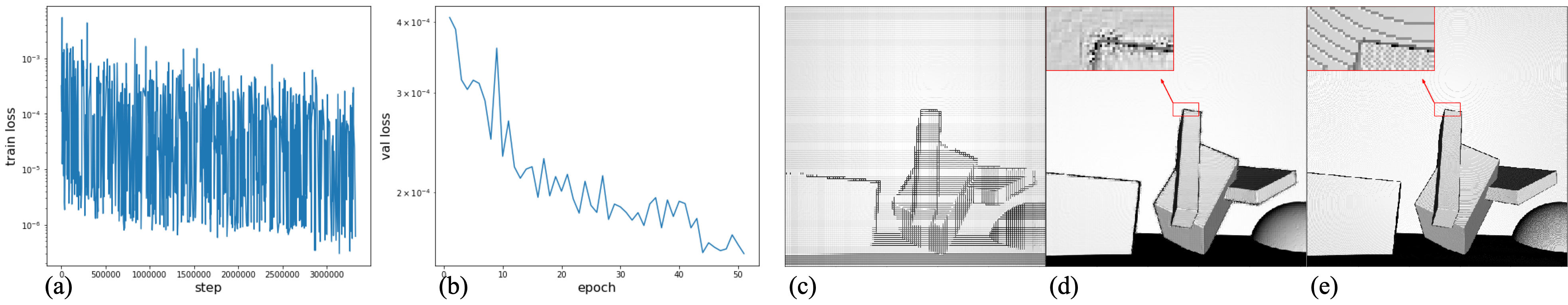
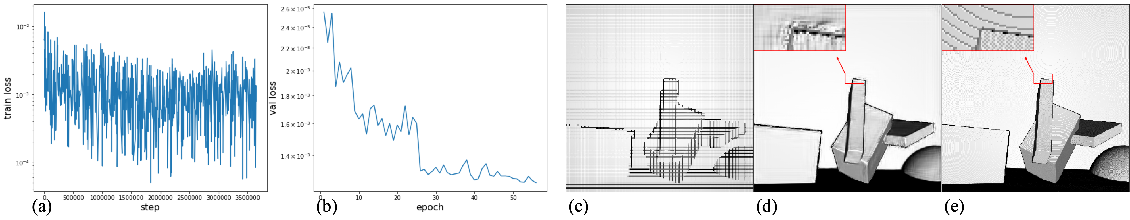
Figure 1: Typical pre-training results using GDSR: (a): train loss dynamics; (b): validation loss dynamics, log-scale; (c): initial approximation (network input); (d): reconstructed depth image; (e): ground-truth.

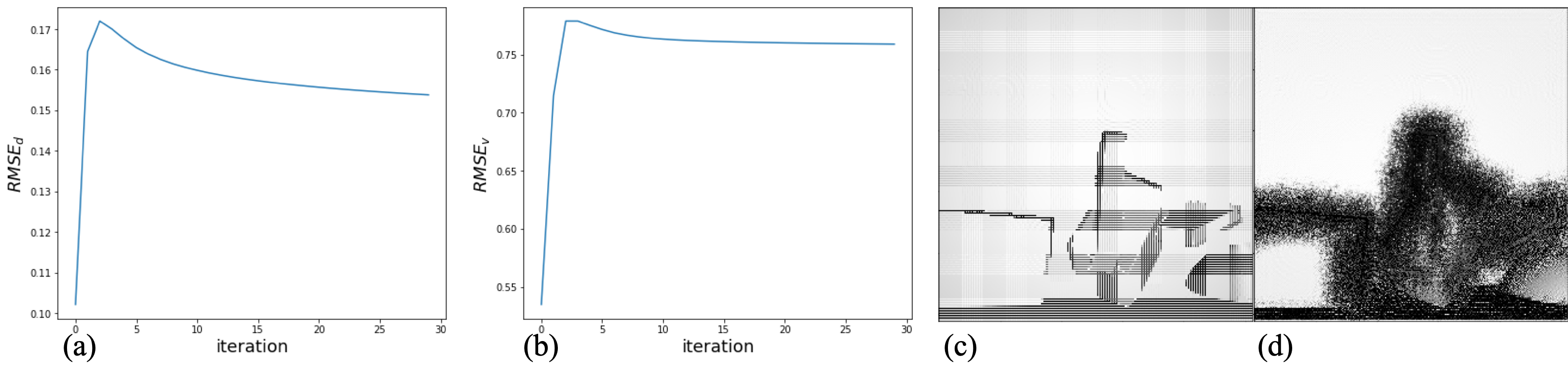
Figure 2: Typical pre-training results using noisy GDSR: (a): train loss dynamics; (b): validation loss dynamics, log-scale; (c): initial approximation (network input); (d): reconstructed depth image; (e): ground-truth.

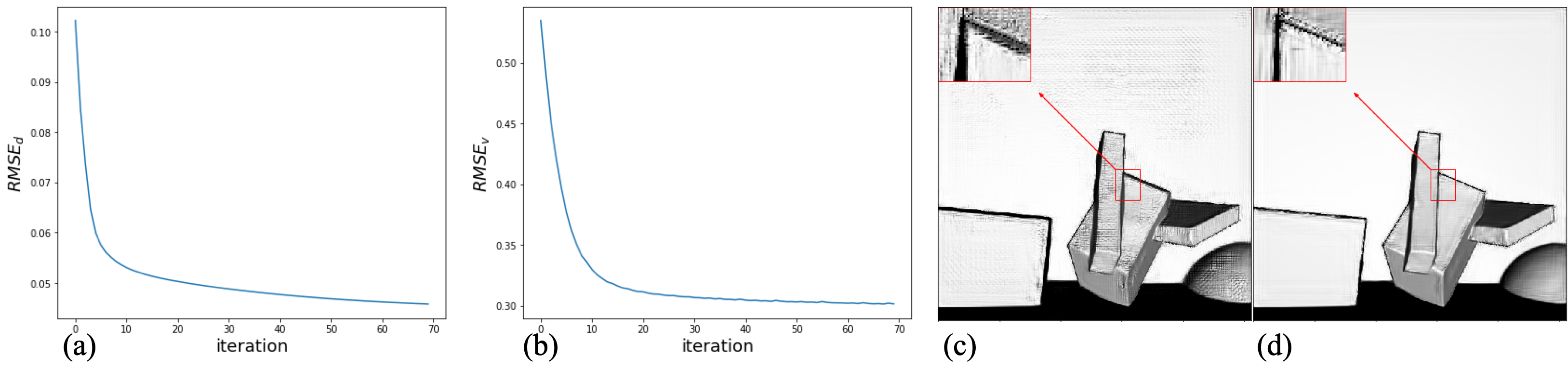
Figure 3: Typical optimization results using networks pre-trained on GDSR: (a): RMSE_d to ground-truth dynamics; (b): RMSE_v to ground-truth dynamics; (c): initial approximation; (d): optimization result (30 iterations).

Figure 4: Typical optimization results using networks pre-trained on noisy GDSR: (a): RMSE_d to ground-truth dynamics; (b): RMSE_v to ground-truth dynamics; (c): initial approximation; (d): optimization result (70 iterations).

To effectively guide optimization in (2), network parameters $\mathbb{V}$ must be learned using the available training data before any optimization may happen (we assume that non-linearities $\sigma_{l}$ are not trainable). We consider the two following pre-training schemes.

Scheme 1: Train the network to predict an artifact component from the input depth image. In this scenario, we split a set $X^{\text{HR}}$ of high-resolution training images $x_{i}$ into two disjoint subsets $X^{\text{HR}}_{0}\cup X^{\text{HR}}_{1}$ and compute approximations $\widetilde{x}_{i}=F^{+}(F(x_{i}))$ for each $x_{i}\in X^{\text{HR}}_{1}$, using an upsampling operator $F^{+}$ (a pseudo-inverse of $F$). The network then trains to predict a residual $r_{i}=x_{i}-\widetilde{x}_{i}$ from the input approximation $\widetilde{x}_{i}$ for images in $X^{\text{HR}}_{1}$, or an exactly zero image for images in $X^{\text{HR}}_{0}$. A simple regularizer based on this network is a Euclidean norm of the predicted residual: $\mathcal{R}(x)=\|\Phi_{\mathbb{V}}(x)\|_{2}^{2}$.

Scheme 2: An alternative approach, which we experimentally observed to aid convergence, is to train the model to directly predict ground-truth depth images given either an input approximation or a ground-truth image. In this scenario, the network is trained to output the same image as input $x_{i}$ for images in $X^{\text{HR}}_{0}$, and an ideal $x_{i}$ from input approximation $\widetilde{x}_{i}$ for images in $X^{\text{HR}}_{1}$. We attribute the advantages of this approach to the benefit of having inputs of similar scale. A similar approach is employed by [Obmann et al., 2019]. We then keep the idea of penalizing images with artifacts in the design of regularizer, which is defined as $\mathcal{R}(x)=\|\Phi_{\mathbb{V}}(x)-x\|_{2}^{2}$.

NETT is guaranteed to converge to a unique and stable solution provided that certain analytic conditions hold [Li et al., 2020]. We report a detailed analysis in the context of our task in the Appendix.

4 EXPERIMENTS

4.1 Toy Examples: GDSR and SimGeo

We start by implementing our approach on simple synthetic depth images, using the dataset from [Riegler et al., 2016], that we denote GDSR. It consists of scenes containing randomly placed cubes, spheres and planes in varying poses and dimensions. Here and below, we visualize 3D scenes as renderings of corresponding depth maps, obtaining these using a simple normals-based method [Voynov et al., 2019].

We train two CNNs to predict residuals in upscaled depth images according to Scheme 1 (i.e., the CNN predicts the artifact part of the training instances): one using the original depth images and another using the noise-augmented depth images, and perform optimization using the two trained models as regularizers. To optimize for a final depth image, we minimize a sum of the squared $L_{2}$-norm data fidelity term and the squared $L_{2}$-norm of network output:

$$\frac{1}{2}\|F(x)-y\|_{2}^{2}+\alpha\|\Phi_{\mathbb{V}}(x)\|_{2}^{2}\rightarrow\min_{x}.$$ (4)

Since the network is trained to output artifact part of the depth maps for visualization of its performance we use rendering of sum of network input and network output, which should approximate ground-truth depth map.

While we are able to train efficient estimators of residuals using both clean and noise-augmented images, as shown in Figures 4–4, using the noise augmentations proves to have a major effect on the optimization performance (see Figures 4–4). More specifically, we find that regularizing optimization in (4) with the network trained on clean synthetic images leads to a bad solution (see Figures 4 (c)–(d)).

Moreover, we discover that the DSRNETT loss function correlates poorly with RMSE_d, the standard root-mean-squared (RMS) error capturing per-pixel differences between depth maps, and perceptual measure RMSE_v [Voynov et al., 2019], defined as the RMS difference between renderings capturing visual differences between 3D surfaces represented as depth maps. Both RMSE_d and RMSE_v represent measures commonly used in evaluating depth map processing performance (see inset Figure 5).

Eventually, optimization resulted in only a marginal improvement for validation samples from GDSR (see Figures 4 (c)–(d)). We hypothesize that this stems from a limited capacity in our network, and seek to increase it in Section 4.2.

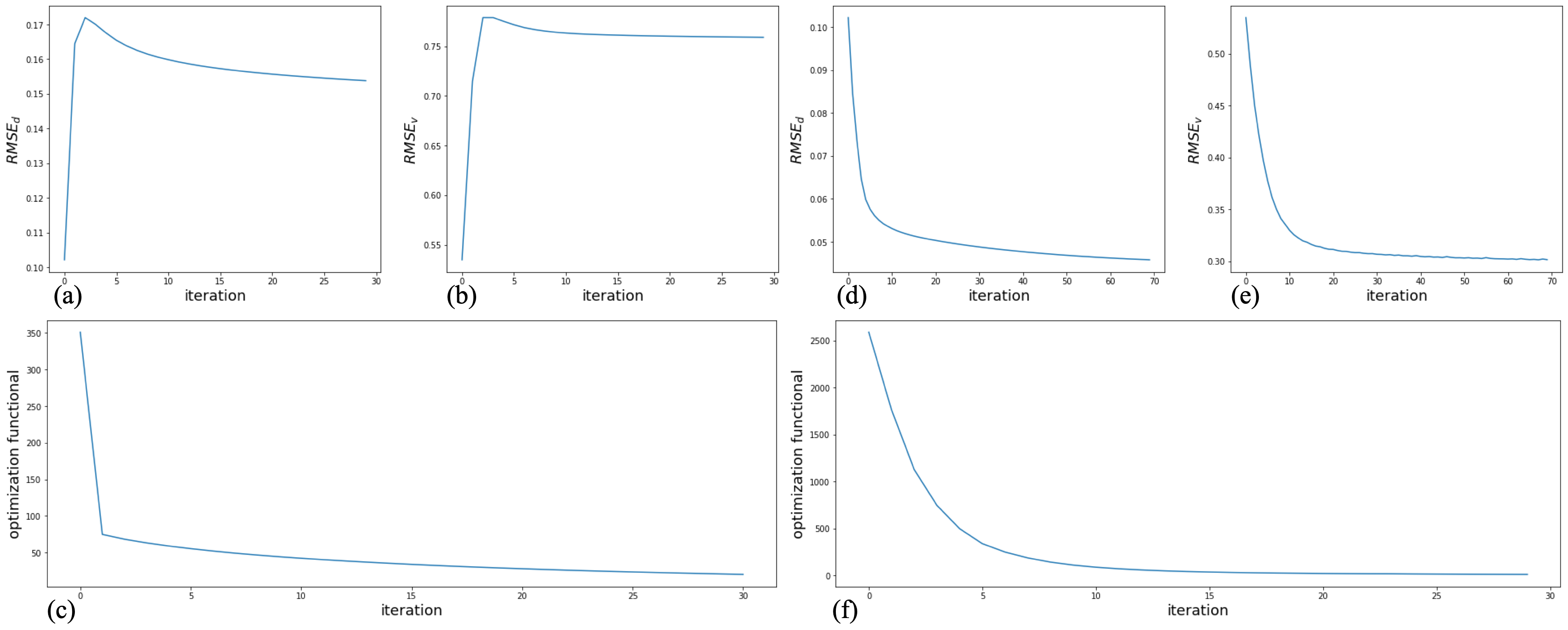
Figure 5: Pre-training on clean data (a)–(c) leads to optimization results where the DSRNETT loss function (4) does not correlate well with the commonly used RMSE_d and RMSE_v measures. Pre-training with noise-augmented data (d)–(f) yields more predictable optimization dynamics.

Implementation details. We obtain $128\times 128$ high-resolution training samples by splitting each image from GDSR  dataset into 16 patches. For 50% of these high-resolution patches, we generate their low-resolution counterparts, choosing $F$ as a box downsampling method with a scaling factor of 4, and obtain approximations $\widetilde{x}$ by applying the pseudo-inverse $F^{+}$ as an upsampling operator. In total, we obtained 128K patches for training and 32K for validation.

We employ a U-Net-like architecture [Ronneberger et al., 2015]. In order to satisfy the coercivity condition for the regularizer term, which is stated by [Li et al., 2020] to be the most restrictive one, we replace ReLU activation function in network architecture with leaky ReLU. We train by optimizing MSE loss using Adam [Kingma and Ba, 2015] for ${\sim}70$ epochs using a batch size of 2.

We perform optimization in (4) using the incremental gradient descent algorithm following [Li et al., 2020]. Thus, optimization consisted of two steps: gradient descent step for data fidelity term with weight $s$ and gradient descent step for regularizer term with weight $s\cdot\alpha$, done with the use of backpropagation algorithm. We also choose the step weights, following [Li et al., 2020]. Yet in contrast, we do not use a zero image as initial approximation, but start optimization from approximation of ground-truth depth map, derived by upsampling $y$, since the network is trained on similar train samples.

To train the network with noisy data, we add Gaussian noise with variance equal to $0.05$ to all pixels in input depth images.

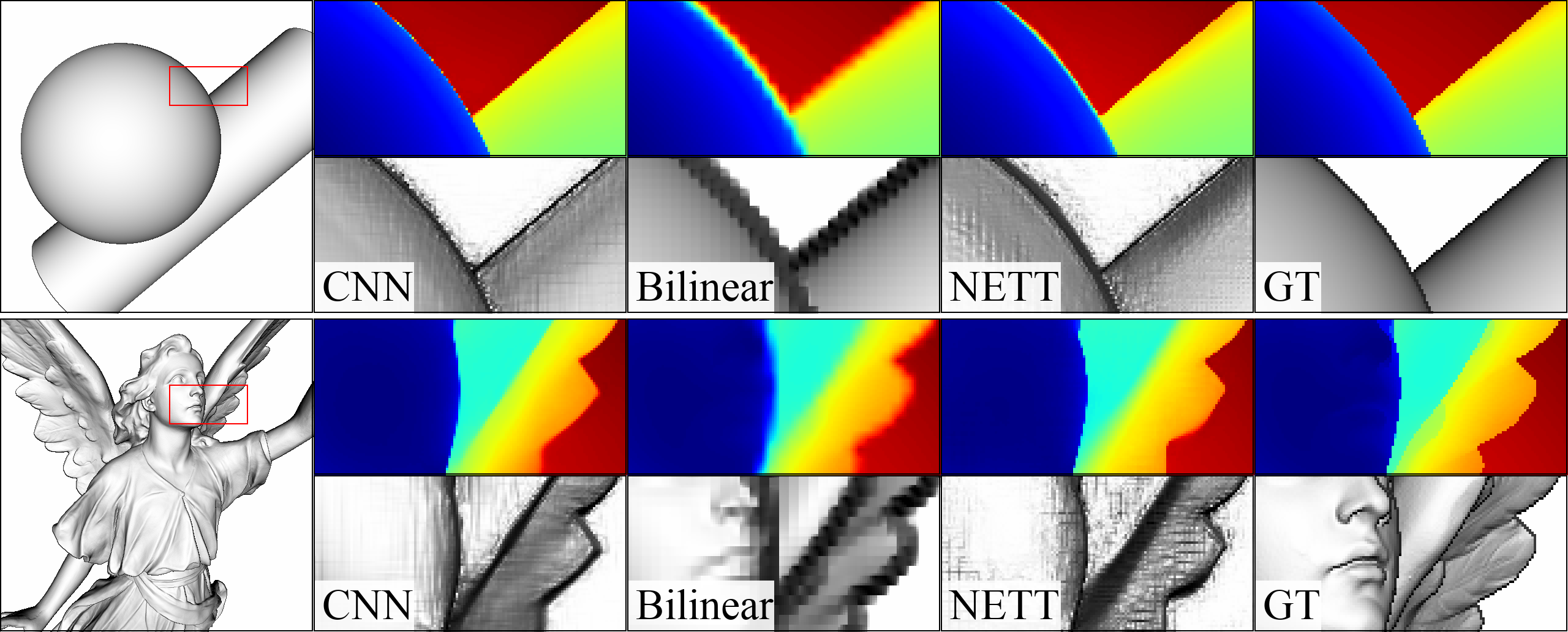
Figure 6: Performance of NETT approach in comparison to underlying network (CNN) and Bilinear interpolation on samples from SimGeo for a network pre-trained on GDSR  with added noise. For each sample - First row: depth maps in pseudo-colour; Second row: renderings in grayscale.

Due to the low complexity of the training dataset, network was pre-trained very well and optimization did not improve network result for validation samples from GDSR. On the other hand, for geometrically more complex synthetic scenes from SimGeo [Voynov et al., 2019] dataset network, pre-trained on GDSR, output poor result and NETT approach was not working correctly; see Figure 6 for comparison of approach performance with underlying network and bilinear interpolation on simple and complex synthetic scenes. According to these suggestions we decided to reimplement NETT with stronger network architecture, using complex synthetic and real-world scenes for pre-training.

4.2 Complex Synthetic and Real-world Scenes: MPI Sintel  and Middlebury

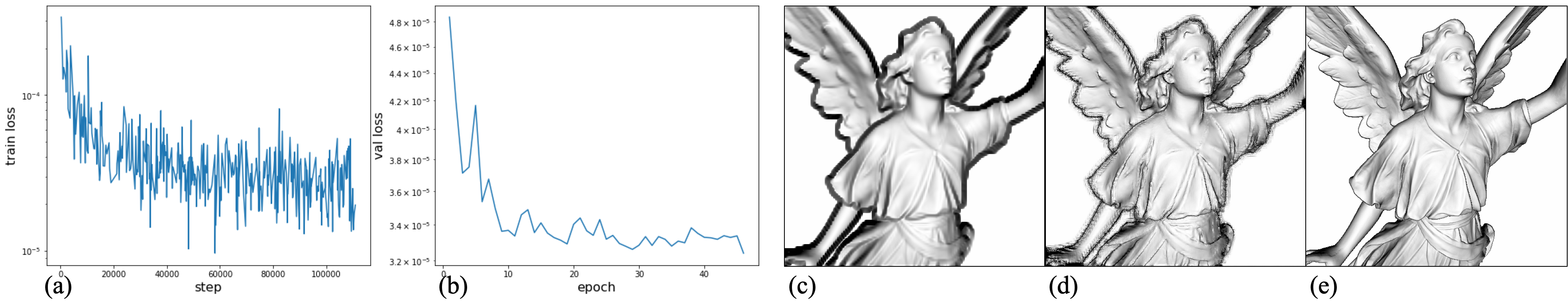
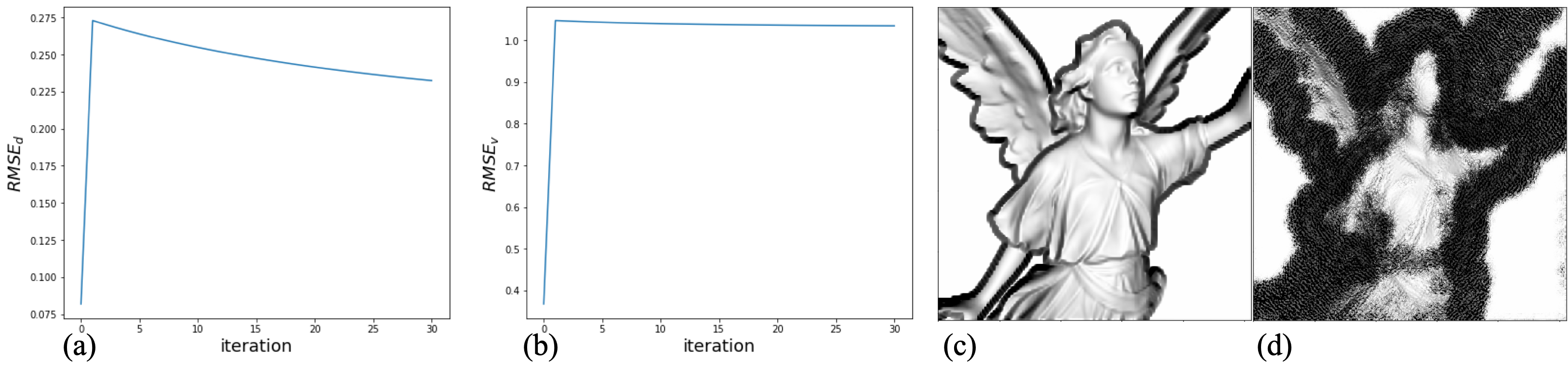
Figure 7: Typical pre-training results using Middlebury 2014 / MPI Sintel (test sample from SimGeo): (a): train loss dynamics; (b): validation loss dynamics, log-scale; (c): input approximation (network input); (d): reconstructed depth image; (e): ground-truth image.

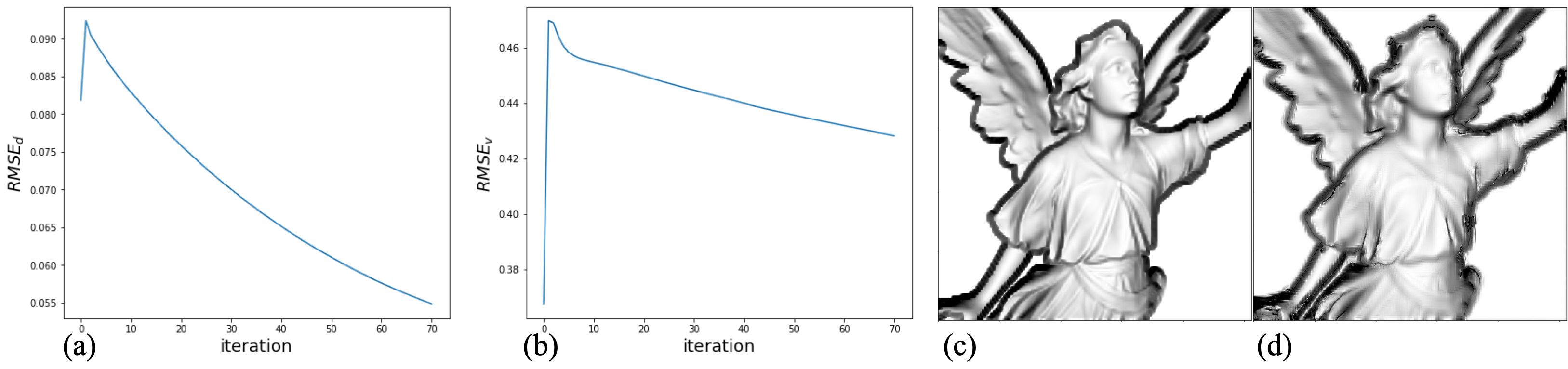
Figure 8: Typical optimization results using networks pre-trained on Middlebury 2014  and MPI Sintel: (a): RMSE_d to ground-truth dynamics; (b): RMSE_v to ground-truth dynamics; (c): initial approximation; (d): optimization result (30 iterations).

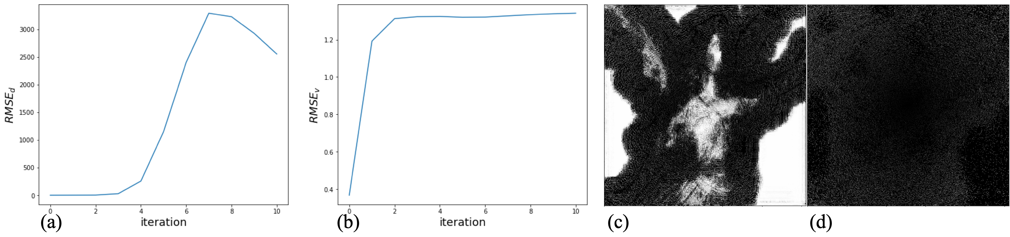
Figure 9: Typical optimization results using networks pre-trained on noisy Middlebury 2014  and MPI Sintel: (a): RMSE_d to ground-truth dynamics; (b): RMSE_v to ground-truth dynamics; (c): initial approximation; (d): optimization result (70 iterations).

Figure 10: Typical optimization results using networks pre-trained on Middlebury 2014  and MPI Sintel  augmented using linear interpolation between GT and approximation: (a): RMSE_d to ground-truth dynamics; (b): RMSE_v to ground-truth dynamics; (c): initial approximation; (d): optimization result (7 iterations).

To study our approach in a full-scale setting, we use data collections and network architectures with larger complexity. More specifically, we use U-MSG-Net, a U-Net-like version of the MSG-Net architecture [Hui et al., 2016] that has demonstrated good performance for depth SR due to the effective use of RGB guidance (see Appendix for more details). For training our network, we use MPI Sintel [Butler et al., 2012] and Middlebury 2014 [Scharstein et al., 2014] datasets, both providing RGB-D images. MPI Sintel  contains complex scenes retrieved from a naturalistic 3D animated short film, while Middlebury 2014 consists of complex high-quality real images captured with a structured light system.

Due to the difficulties with optimization convergence, that we discuss further, in addition to training the network according to Scheme 1 we experimented with training according to Scheme 2, where the goal is to predict a reconstructed image given an input approximation. We observed that Scheme 2 leads to better convergence in comparison to Scheme 1 and further provide results for Scheme 2. For optimization, we accordingly set the regularizer to $\mathcal{R}(x)=\|\Phi_{\mathbb{V}}(x)-x\|^{2}_{2}$, re-using the general framework described previously.

We do not explicitly account for the coercivity condition of the architecture, since [Li et al., 2020] provides ways to obtain coercivity for an arbitrary architecture, e.g., using skip connection between network input and output, as we discuss further.

Data augmentation. To aid generalization, we study a number of data augmentation strategies aiming to expand the training domain, summarized in Table 1.

Training with noisy inputs. We train the network on input depth images augmented with different variations of additive random noise (lines 2, 4-6 in the table).

Training with both noisy inputs and targets. Aiming to increase network robustness, we train the network to predict noisy ground-truth depth from noisy ground-truth, keeping target noise variance smaller than that of input noise (line 7).

Training with input in-between approximation and ground truth. The regularizer $\mathcal{R}(x)$ is designed to push $x$ to ground-truth data manifold, approximated by $\Phi_{\mathbb{V}}(x)$. Based on the derivation in Appendix, we hypothesize that, in contrast to this desired behaviour, the optimization of the regularizer also pushes the output of the network in the undesired direction. To prevent that, we additionally train the network on the samples, where the input is the result of one step of optimization with small regularizer step size $s\cdot\alpha=0.001$. We also try a simpler strategy to train on random linear interpolation between the approximation and the ground truth as the input.

Additionally, in the experiments with MPI Sintel  and Middlebury 2014  we randomly rotate the patches by $90^{\circ}$. We briefly review the results of these experiments below.

Table 1: Summary of conducted experiments. Mid./Sint. correspond to Middlebury 2014/MPI Sintel.

Pre-training	Net	Scheme	Input augmentation	Optimization	Result	Opt.	$\mathrm{RMSE_{d}}$	$\mathrm{RMSE_{v}}$
GDSR	U-Net	1	—	GDSR	Noisy	✓	✓	✓
GDSR	U-Net	1	Gaussian noise with $\sigma=0.05$	GDSR	OK	✓	✓	✓
Mid./Sint.	U-MSG-Net	2	—	SimGeo	Noisy	✓	✗	✗
Mid./Sint.	U-MSG-Net	2	$\sigma=0.03$	SimGeo	Over-smoothed	✓	✓	✓
Mid./Sint.	U-MSG-Net	2	$\sigma=0.03$, scaled by 0.7 every 10-th epoch	SimGeo	Over-smoothed	✓	✓	✓
Mid./Sint.	U-MSG-Net	2	Additional input samples (+): GT with gaussian noise with $\sigma=\mathrm{MSE(GT,approximation)}$	SimGeo	Same as input	✓	✓	✗
Mid./Sint.	U-MSG-Net	2	+ GT with noise $\epsilon$, and target with noise $\epsilon/10$	SimGeo	Same as input	✓	✓	✗
Mid./Sint.	U-MSG-Net	2	+ random linear interpolation between GT and approximation	SimGeo	Noisy	✗	✗	✗
Mid./Sint.	U-MSG-Net	2	+ with the result after one step of optimization	SimGeo	Same as input	$\checkmark$	✗	✗

Similarly to results in Section 4.1, training without data augmentations results in optimization hitting a bad solution (see Figure 10). Network trained on noisy data tends to produce over-smooth depth maps (see Figure 10). Using noisy data with gradually decreasing noise variance similarly leads to over-smoothed network outputs and optimization result. Expanding training data with intermediate optimization results did not alleviate difficulties with optimization convergence. Moreover, in some instances, this resulted in well trained network, but exploding optimization, yielding extremely noisy results (see Figure 10). Training using noisy targets again led to over-smoothed network outputs and aggravated artefacts in optimization results.

Implementation details. We construct training dataset similar to the one proposed in [Hui et al., 2016] for training MSG-Net  but appropriate for use within DSRNETT. We split all images into patches of size $64\times 64$. For all patches we calculate intensity, corresponding to RGB component. For half of the patches we generate low-resolution depth using box downsampling method with a scaling factor of 4, and obtain approximations using a bilinear upsampling method instead of pseudo-inverse of box downsampling, since the former produces patches that are more relevant for training MSG-Net. Finally, following our Scheme 2, we train the model using the high-frequency (HF) components of intensity and depth of generated patches as inputs, and HF components of ground-truth depth and intensity as targets. For simplicity we further omit the fact that model is trained on HF components and its inputs and outputs contain not only depth, but also intensity part, since it is not changed during training or optimization. In total, training was performed on $75$K patches with $15$K patches used for validation. We train by optimizing MSE loss using Adam for ${\sim}120$ epochs with a batch size of 128.

We experimentally set minimum noise variance to $0.03$. In experiment with noisy targets for network inputs we added Gaussian noise with variance $\sigma=0.001$; each target variance of noise was defined as $\text{MSE}(\sigma,0)$, divided by $10$.

Ensuring coercivity of regularizer. According to remark in [Obmann et al., 2019] in order to ensure coercivity of regularizer in experiments with U-MSG-Net, we employed skip-connection between network input and output and define regularizer as $\mathcal{R}(x)=\|\Phi_{\mathbb{V}}(x)-x\|^{2}+\|x\|^{2}.$ We have checked, that such regularizer design does not help to solve optimization issues and concluded, that optimization convergence to undesired local minimum was not lead by possible regularizer non-coercivity.

5 DISCUSSION

In this work, we performed an adaptation of NETT [Li et al., 2020], an approach to image processing leveraging data-driven regularizers, for the depth super-resolution (SR) task. We have validated that our formulation of depth SR meets all theoretical requirements of NETT, including the restrictive coercivity condition. Furthermore, we were able to train an efficient residual estimator deep network in all experimental cases. Unexpectedly, we have discovered subsequent optimization to converge to the bad minimum in most experiments despite multiple efforts to increase network stability by varying the training dataset, applying data augmentations, selecting different models, or considering various formulations of the optimization task.

Our results raise questions regarding the use of learned regularizers in the context of depth SR (or image-based tasks), which may represent promising future research directions. More specifically,

1. What is the required form of the regularization term that would allow effective optimization?

2. What are the characteristic features of image-based tasks that might prevent optimization methods such as [Li et al., 2020] from converging to good solutions?

3. What is the “right” training procedure for the regularizer?

APPENDIX

Network Tikhonov Regularization Assumptions

[Li et al., 2020] prove well-posedness and convergence of NETT regularization, provided that certain assumptions on regularizer and data fidelity term hold.

We have tried to ensure fulfillment of this conditions in our work. Conditions on data fidelity term are not restrictive and hold for squared $L_{2}$-norm distance, while the conditions on regularizer term include:

1. Regularizer $\mathcal{R}(x)=\psi(\Phi_{\mathbb{V}}(x))$ is weakly lower semicontinuous, which is guaranteed by conditions:

   • Linear operators $\mathbb{A}_{l}$ are bounded;

   • Non-linearities $\sigma_{l}$ are weakly continuous;

   • Scalar functional $\psi$ is weakly lower-semicontinuous;

2. $\mathcal{R}(x)$ is coercive, i.e. $\lim_{\|x\|\rightarrow\infty}\mathcal{R}(x)=0$.

U-Net-type and U-MSG-Net  architectures include convolution operations and batch normalizations, that are bounded linear operations, and max pooling, leaky ReLU and upsampling operations, that are weakly continuous and coercive non-linearities. We use squared $L_{2}$-norm distance as weakly lower semi-continuous scalar functional $\psi$. We note that the number of parameters in the U-Net  model is close to 7M, while in the U-MSG-Net  it is around 700K.

Several ways to obtain coercivity of the regularizer are discussed in [Li et al., 2020]. One way is to ensure layer-wise coercivity, i.e. use coercive non-linearities $\sigma_{l}$ and linear operators $\mathbb{A}_{l}$, satisfying the inequality:

$$\exists c_{l}\in[0,\infty)\forall x\in X:\;\|x\|\leq c_{l}\|A_{l}x\|.$$ (5)

We relied on this approach in experiments with U-Net-type architecture. Since U-MSG-Net  contains non-coercive parametric ReLU non-linearities, we used another way to obtain network coercivity by exploiting skip connection between network input and output, see ”Ensuring coercivity of regularizer” in Section 4.2.

Specifically, fulfillment of presented conditions guarantee existence of a solution, stability and convergence for optimization problem (2). Stability of the method corresponds to continuous dependence of the solutions $x$ of optimization problem (2) on input $y$. Convergence of the method states, that while noise level $\delta_{k}$ in inputs $y_{\delta_{k}}$ decreases to zero, sequence $x_{k}$ of corresponding solutions weakly converges to the $\mathcal{R}(\cdot)$-minimizing solution $x_{+}$ of $F(x)=y_{0}$, if it is unique.

Experiments

Figures 11 and 12 represent architectures of networks, used in experiments in Sections 4.1 and 4.2 respectively.

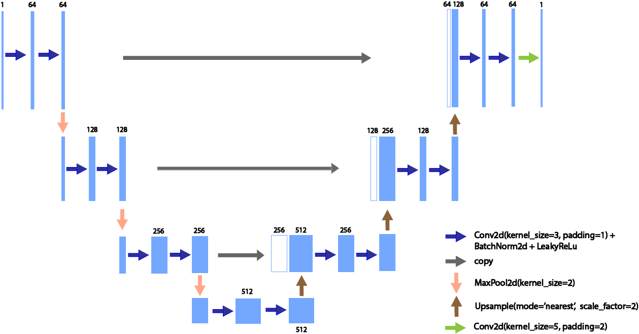
Figure 11: U-Net-type architecture.

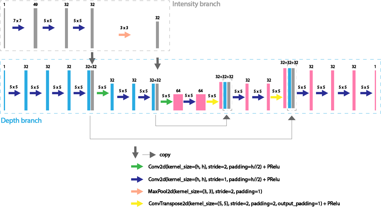
Figure 12: U-MSG-Net  architecture.

Training on Intermediate Optimization Results as Input

In our experiments we use approximation $\widetilde{x}$, i.e. upsampled low-resolution version of ground-truth depth, as optimization initial approximation. We suppose, that optimization approximation is not significantly changed after the first data fidelity gradient descent step and treat $\widetilde{x}$ as its result.

Then after the regularizer gradient descent step we obtain approximation $x_{1}$:

$$x_{1}=\widetilde{x}-s\cdot\alpha\cdot\frac{d\mathcal{R}(x)}{x}|_{x=\widetilde{x}}$$ (6)

If network is trained to predict ground-truth depth given both $\widetilde{x}$ or $x_{1}$, then regularizer gradient descent step would not move optimization approximation to the direction of $x_{1}$:

$$\|\Phi_{\mathbb{V}}(x_{1})-x_{1}\|^{2}=\|\Phi_{\mathbb{V}}(\widetilde{x})-\widetilde{x}+s\cdot\alpha\cdot\frac{d\mathcal{R}(x)}{x}|_{x=\widetilde{x}}\|^{2}$$

$$\geq\|\Phi_{\mathbb{V}}(\widetilde{x})-\widetilde{x}\|^{2}+\|s\cdot\alpha\cdot\frac{d\mathcal{R}(x)}{x}|_{x=\widetilde{x}}\|^{2}$$

$$\geq\|\Phi_{\mathbb{V}}(\widetilde{x})-\widetilde{x}\|^{2}.$$

Thus, we come to idea to add optimization first step approximation for small $s\cdot\alpha=0.001$ to the training samples.

REFERENCES

- Arridge et al., 2019 Arridge, S., Maass, P., Öktem, O., and Schönlieb, C.-B. (2019). Solving inverse problems using data-driven models. Acta Numerica, 28:1–174.
- Butler et al., 2012 Butler, D. J., Wulff, J., Stanley, G. B., and Black, M. J. (2012). A naturalistic open source movie for optical flow evaluation. In Fitzgibbon, A., Lazebnik, S., Perona, P., Sato, Y., and Schmid, C., editors, Computer Vision – ECCV 2012, volume 7577 of LNCS, pages 611–625, Berlin, Heidelberg. Springer Berlin Heidelberg.
- Chen et al., 2013 Chen, Y., Pock, T., Ranftl, R., and Bischof, H. (2013). Revisiting loss-specific training of filter-based mrfs for image restoration. In Weickert, J., Hein, M., and Schiele, B., editors, German Conference on Pattern Recognition, volume 8142 of LNCS, pages 271–281, Berlin, Heidelberg. Springer.
- De los Reyes et al., 2017 De los Reyes, J. C., Schönlieb, C.-B., and Valkonen, T. (2017). Bilevel parameter learning for higher-order total variation regularisation models. Journal of Mathematical Imaging and Vision, 57(1):1–25.
- Gatys et al., 2016 Gatys, L., Ecker, A., and Bethge, M. (2016). A neural algorithm of artistic style. Journal of Vision, 16(12):326–326.
- Gou et al., 2021 Gou, J., Yu, B., Maybank, S. J., and Tao, D. (2021). Knowledge distillation: A survey. International Journal of Computer Vision, 129(6):1789–1819.
- Haefner et al., 2020 Haefner, B., Peng, S., Verma, A., Quéau, Y., and Cremers, D. (2020). Photometric depth super-resolution. IEEE Transactions on Pattern Analysis and Machine Intelligence, 42(10):2453–2464.
- Haefner et al., 2018 Haefner, B., Quéau, Y., Möllenhoff, T., and Cremers, D. (2018). Fight ill-posedness with ill-posedness: Single-shot variational depth super-resolution from shading. In 2018 IEEE/CVF Conference on Computer Vision and Pattern Recognition, pages 164–174.
- Hui et al., 2016 Hui, T.-W., Loy, C. C., and Tang, X. (2016). Depth map super-resolution by deep multi-scale guidance. In Leibe, B., Matas, J., Sebe, N., and Welling, M., editors, European Conference on Computer Vision – ECCV 2016, volume 9907 of LNCS, pages 353–369, Cham. Springer International Publishing.
- Johnson et al., 2016 Johnson, J., Alahi, A., and Fei-Fei, L. (2016). Perceptual losses for real-time style transfer and super-resolution. In European conference on computer vision, pages 694–711. Springer.
- Kingma and Ba, 2015 Kingma, D. P. and Ba, J. (2015). Adam: A method for stochastic optimization. In ICLR (Poster).
- Li et al., 2020 Li, H., Schwab, J., Antholzer, S., and Haltmeier, M. (2020). NETT: Solving inverse problems with deep neural networks. Inverse Problems, 36(6):065005.
- Lunz et al., 2018 Lunz, S., Öktem, O., and Schönlieb, C.-B. (2018). Adversarial regularizers in inverse problems. In Proceedings of the 32nd International Conference on Neural Information Processing Systems, NIPS’18, pages 8516–8525, Red Hook, NY, USA. Curran Associates Inc.
- Obmann et al., 2019 Obmann, D., Nguyen, L., Schwab, J., and Haltmeier, M. (2019). Sparse -regularization of inverse problems using deep learning. arXiv:1908.03006.
- Riegler et al., 2016 Riegler, G., Ferstl, D., Rüther, M., and Bischof, H. (2016). A deep primal dual for guided depth super-resolution. In British Machine Vision Conference, United Kingdom. The British Machine Vision Association.
- Ronneberger et al., 2015 Ronneberger, O., Fischer, P., and Brox, T. (2015). U-net: Convolutional networks for biomedical image segmentation. In Navab, N., Hornegger, J., Wells, W. M., and Frangi, A. F., editors, Medical Image Computing and Computer-Assisted Intervention – MICCAI 2015, volume 9351 of LNCS, pages 234–241, Cham. Springer International Publishing.
- Scharstein et al., 2014 Scharstein, D., Hirschmüller, H., Kitajima, Y., Krathwohl, G., Nešić, N., Wang, X., and Westling, P. (2014). High-resolution stereo datasets with subpixel-accurate ground truth. In Jiang, X., Hornegger, J., and Koch, R., editors, German Conference on Pattern Recognition, volume 8753 of LNCS, pages 31–42, Cham. Springer International Publishing.
- Song et al., 2020 Song, X., Dai, Y., Zhou, D., Liu, L., Li, W., Li, H., and Yang, R. (2020). Channel attention based iterative residual learning for depth map super-resolution. In 2020 IEEE/CVF Conference on Computer Vision and Pattern Recognition (CVPR), pages 5630–5639.
- Voynov et al., 2019 Voynov, O., Artemov, A., Egiazarian, V., Notchenko, A., Bobrovskikh, G., Zorin, D., and Burnaev, E. (2019). Perceptual deep depth super-resolution. In Proceedings of the IEEE International Conference on Computer Vision, pages 5653–5663.
- Zacharov et al., 2019 Zacharov, I., Arslanov, R., Gunin, M., Stefonishin, D., Bykov, A., Pavlov, S., Panarin, O., Maliutin, A., Rykovanov, S., and Fedorov, M. (2019). “zhores”—petaflops supercomputer for data-driven modeling, machine learning and artificial intelligence installed in skolkovo institute of science and technology. Open Engineering, 9(1):512–520.