Learned ISTA with Error-based Thresholding for Adaptive Sparse Coding

Abstract

Drawing on theoretical insights, we advocate an error-based thresholding (EBT) mechanism for learned ISTA (LISTA), which utilizes a function of the layer-wise reconstruction error to suggest a specific threshold for each observation in the shrinkage function of each layer. We show that the proposed EBT mechanism well disentangles the learnable parameters in the shrinkage functions from the reconstruction errors, endowing the obtained models with improved adaptivity to possible data variations. With rigorous analyses, we further show that the proposed EBT also leads to a faster convergence on the basis of LISTA or its variants, in addition to its higher adaptivity. Extensive experimental results confirm our theoretical analyses and verify the effectiveness of our methods.

Index Terms—  Sparse Coding, Learned ISTA, Adaptivity

1 Introduction

The core problem of sparse coding is to deduce the high-dimensional sparse code from the low-dimensional observation. The basic assumption can be formulated as $y=Ax^{\star}+\varepsilon$, where $y\in\mathbb{R}^{m}$ is the observation corrupted by the inevitable noise $\varepsilon\in\mathbb{R}^{m}$, $x^{\star}\in\mathbb{R}^{n}$ is the sparse code to be estimated, and $A\in\mathbb{R}^{m\times n}$ is an over-complete dictionary matrix. The main challenge to estimate $x$ is its ill-posed nature because of over-complete modeling, i.e., $m<n$. A possible solution is to solve the LASSO problem formulated as $\min_{x}\|y-Ax\|_{2}+\lambda\|x\|_{1}$ using the iterative shrinking thresholding algorithm (ISTA) [1]. To achieve faster convergence, Learned ISTA (LISTA) [2] was then proposed in the deep learning era, in which the architecture of the deep neural network (DNN) followed the iterative process of ISTA. The thresholding mechanism was then modified to the learned thresholds in shrinkage functions of DNNs.

Yet, LISTA and many other deep networks based on LISTA [3, 4, 5, 6, 7, 8] suffer the issue that the thresholds were shared among all training samples, which means they lacked adaptability to the variety of training samples and robustness to outliers. Also, it leads to poor generalization to test data with a different distribution (or sparsity) from the training data. To address the above issues, we propose an error-based thresholding (EBT) mechanism of LISTA-based models to improve their adaptivity. EBT introduces a function of the evolving estimation error to provide each threshold in the shrinkage functions in the model. It has no extra learnable parameter compared with original LISTA-based models, yet shows significantly better performance.

2 Preliminary Knowledge

The update rule of ISTA is

$$x^{(t+1)}=\mathrm{sh}_{\lambda/\gamma}((I-A^{T}A/\gamma)x^{(t)}+A^{T}y/\gamma),\quad\forall t\geq 0,$$ (1)

where $\mathrm{sh}_{b}(x)=\mathrm{sign}(x)(|x|-b)_{+}$ is a shrinkage function with a threshold $b\geq 0$ and $(\cdot)_{+}=\max\{0,\cdot\}$, $\gamma$ is the maximal eigenvalue of the symmetric matrix $A^{T}A$. LISTA kept the update rule of ISTA but learned parameters via end-to-end training. Its inference process can be formulated as

$$x^{(t+1)}=\mathrm{sh}_{b^{(t)}}(W^{(t)}x^{(t)}+U^{(t)}y),$$ (2)

where $\Theta=\{W^{(t)},U^{(t)},b^{(t)}\}_{t=0,\dots,d}$ is a set of learnable parameters. Specifically, $b^{(t)}$ is the layer-wise learnable threshold shared among all samples, which is of our particular interest in this paper. LISTA has been proved to converge linearly with partial weight coupling [3], i.e., $W^{(t)}=I-U^{(t)}A$, thus Eq. (2) can be written as

$$x^{(t+1)}=\mathrm{sh}_{b^{(t)}}((I-U^{(t)}A)x^{(t)}+U^{(t)}y).$$ (3)

Support selection was further introduced to modify LISTA [3]. We select entries with largest $p^{(t)}$ (in percentage) magnitudes in vector $x$ as support set $S_{p^{(t)}}$. The entries in support set do not pass the thresholding and keep them values unchanged. Formally, we define $\mathrm{shp}_{(b^{(t)},p^{(t)})}$ as the thresholding operator with support selection, the update rule is then formulated as

$$x^{(t+1)}=\mathrm{shp}_{(b^{(t)},p^{(t)})}((I-U^{(t)}A)x^{(t)}+U^{(t)}y),$$ (4)

where $p^{(t)}$ is a hyper-parameter and it increases from lower layers to higher layers. $p^{(t)}$ can be set as $p^{(t)}=\min(p\cdot t,p_{max})$, where $p$ is the positive scalar and $p_{max}$ is the upper bound of the percentage of non-zero elements in $x$. LISTA with support selection is proved to achieve faster convergence in comparison with LISTA [3].

According to the convergence analyses of LISTA and its variants [3, 4, 5, 6], the following equality should hold for the threshold at each layer to ensure linear convergence:

$$b^{(t)}=\mu(A)\sup_{x^{\star}\in\mathcal{S}}\|x^{(t)}-x^{\star}\|_{\phi}$$ (5)

where $\mathcal{S}$ is the training set, $\mu(A)$ is the generalized mutual coherence coefficient of the dictionary matrix $A\in\mathbb{R}^{m\times n}$, and $\phi$ represents the type of the norm which is commonly set as $1$ or $2$. Note that $\mu(A)$ is a crucial term in this paper, here we formally give its definition together with the definition of $\mathcal{W}(A)$ as follows:

Definition 1.

[4] For a matrix $A$, we let $A_{i,:}$ represents the $i$-th row of $A$ and $A_{:,j}$ represents the $j$-th column of $A$. The generalized mutual coherence coefficient of $A$ is $\mu(A)=\inf_{W\in\mathbb{R}^{n\times m},W_{i,:}A_{:,i}=1}\max_{i\neq j}{(W_{i,:}A_{:,j})}$. In addition, we let $\mathcal{W}(A)$ denotes the set of the matrices which can achieve $\mu(A)$, which means $\mathcal{W}(A)=\{W\in\mathbb{R}^{n\times m}|\max_{i\neq j}{(W_{i,:}A_{:,j})}=\mu(A),W_{i,:}A_{:,i}=1,\forall i\}$.

3 Methods

In LISTA and many of its variants, the threshold $b^{(t)}$ is commonly treated as a learnable parameter. As demonstrated in Eq. (5), $b^{(t)}$ should be proportional to the upper bound of the estimation error of the $t$-th layer in the noiseless case to ensure fast convergence [3, 4, 5, 6]. Thus, some outliers or extreme training samples greatly influence the value of $b^{(t)}$, making the obtained threshold not fit the majority of the data.

In order to solve this problem, we propose to disentangle the reconstruction error term from the learnable part of the threshold and introduce adaptive thresholds for LISTA and related networks. We attempt to rewrite the threshold at the $t$-th layer as something like $b^{(t)}=\rho^{(t)}\|x^{(t)}-x^{\star}\|_{\phi},$ where $\rho^{(t)}$ is a layer-specific learnable parameter. However, the ground-truth $x^{\star}$ is actually unknown for the inference process. Therefore, we need to find an alternative formulation. Notice that in the noiseless case, it holds that $Ax^{(t)}-y=A(x^{(t)}-x^{\star})$. Also, we know $U^{(t)}\in\mathcal{W}(A)$ is desirable according to prior works [3, 4, 5, 6], which means $U^{(t)}A$ approximates the identity matrix. Thus, we propose our EBT-LISTA, which is formulated as

$$x^{(t+1)} =\mathrm{sh}_{b^{(t)}}((I-U^{(t)}A)x^{(t)}+U^{(t)}y),$$ (6)

$$b^{(t)} =\rho^{(t)}\|U^{(t)}(Ax^{(t)}-y)\|_{\phi}.$$

Note that only $\rho^{(t)}$ and $U^{(t)}$ are learnable parameters in the above formulation, thus our EBT-LISTA actually introduces no extra parameters compared with the original LISTA.

We can also apply our EBT mechanism to LISTA with support selection [3] by keeping support selection operation and replacing the fixed threshold, which is formulated as

$$x^{(t+1)} =\mathrm{shp}_{(b^{(t)},p^{(t)})}((I-U^{(t)}A)x^{(t)}+U^{(t)}y),$$ (7)

$$b^{(t)} =\rho^{(t)}\|U^{(t)}(Ax^{(t)}-y)\|_{\phi}.$$

4 Theoretical Analysis

In this section, we provide convergence analyses for LISTA and LISTA with support selection. Proof of all our theoretical results can be found in the appendices. We focus on the noiseless case and the main results are obtained under some assumptions of the ground-truth sparse code. Specifically, we here assume that the ground-truth sparse vector $x^{\star}$ is sampled from the distribution $\gamma(B,s)$, i.e., the number of its nonzero elements follow a uniform distribution $U(0,s)$ and the magnitude of its nonzero elements follow an arbitrary distribution in $[-B,B]$. We also assume that $s$ is sufficiently small in our theoretical analysis for error-based thresholding, which means $\mu(A)(2s-1)<1$ to be exact. Note that similar assumptions can also be found in relative works [3, 4, 6, 7].

4.1 EBT mechanism on LISTA

Let us first recall the convergence of LISTA and discuss how our EBT improves LISTA in accelerating convergence.

Lemma 1.

[3] For LISTA formulated in Eq. (3), $x^{\star}$ is sampled from $\gamma(B,s)$. If $s$ is small such that $\mu(A)(2s-1)<1$, $U^{(t)}\in\mathcal{W}(A)$, and $b^{(t)}=\mu(A)\sup_{x^{\star}}\|x^{(t)}-x^{\star}\|_{1}$, the estimation $x^{(t)}$ at the $t$-th layer of LISTA satisfies

$$\|x^{(t)}-x^{\star}\|_{2}\leq sB\exp{(c_{0}t)},$$

where $c_{0}=\log((2s-1)\mu(A))<0$.

Theorem 1.

(Convergence of EBT-LISTA) For EBT-LISTA formulated in Eq. (6) where $\phi=1$, $x^{\star}$ is sampled from $\gamma(B,s)$. If $s$ is small such that $\mu(A)(2s-1)<1$, $U^{(t)}\in\mathcal{W}(A)$ and $\rho^{(t)}=\frac{\mu(A)}{1-\mu(A)s}$, the estimation $x^{(t)}$ at the $t$-th layer satisfies

$$\|x^{(t)}-x^{\star}\|_{2}\leq q_{0}\exp{(c_{1}t)},$$

where $q_{0}<sB$ and $c_{1}<c_{0}$ hold with the probability of $1-\mu(A)s$.

Compared Theorem 1 with Lemma 1, we know that EBT-LISTA converges similarly as the original LISTA. The convergence rate is probably faster and the reconstruction error is probably lower, with $c_{1}<c_{0}$ and $q_{0}<sB$. Since $s$ is assumed to be small such that $\mu(A)(2s-1)<1$, which means $\mu(A)s<0.5$, indicating our EBT achieves superiority in a higher probability. Moreover, in an extremely sparse scenario with $s$ being sufficiently small such that $\mu(A)s\ll 1$, the probability of achieving the superiority is relatively high in theory. Under this circumstance, the desired threshold in EBT-LISTA should be $\mu(A)$ and it is disentangled with the reconstruction error, unlike the desired threshold in original LISTA, i.e., $\mu(A)\sup_{x^{\star}}\|x^{(t)}-x^{\star}\|_{1}$.

4.2 EBT mechanism on LISTA with support selection

There exist many variants of LISTA, and in this subsection, we choose LISTA with support set selection as an example to show how our EBT improves it in theory.

Lemma 2.

(Convergence of LISTA with support selection) For LISTA with support selection formulated in Eq. (4), $x^{\star}$ is sampled from $\gamma(B,s)$. If $s$ is small such that $\mu(A)(2s-1)<1$, $U^{(t)}\in\mathcal{W}(A)$ and $b^{(t)}=\mu(A)\sup_{x^{\star}}\|x^{(t)}-x^{\star}\|_{1}$, there actually exist two convergence phases. In the first phase, i.e., $t\leq t_{0}$, the $t$-th layer estimation $x^{(t)}$ satisfies

$$\|x^{(t)}-x^{\star}\|_{2}\leq sB\exp{(c_{2}t)},$$

where $c_{2}\leq\log((2s-1)\mu(A))$. In the second phase, i.e., $t>t_{0}$, the estimation $x^{(t)}$ satisfies

$$\|x^{(t)}-x^{\star}\|_{2}\leq C\|x^{(t-1)}-x^{\star}\|_{2},$$

where $C\leq s\mu(A)$.

Theorem 2.

(Convergence of EBT-LISTA with support selection) For EBT-LISTA with support selection and $\phi=1$, $x^{\star}$ is sampled from $\gamma(B,s)$. If $s$ is small such that $\mu(A)(2s-1)<1$, $U^{(t)}\in\mathcal{W}(A)$, and $\rho^{(t)}=\frac{\mu(A)}{1-\mu(A)s}$, there exist two convergence phases. In the first phase, i.e., $t\leq t_{1}$, the $t$-th layer estimation $x^{(t)}$ satisfies

$$\|x^{(t)}-x^{\star}\|_{2}\leq q_{1}\exp{(c_{3}t)},$$

where $c_{3}<c_{2}$, $q_{1}<sB$ and $t_{1}<t_{0}$ hold with a probability of $1-\mu(A)s$. In the second phase, i.e., $t>t_{1}$, the estimation $x^{(t)}$ satisfies

$$\|x^{(t)}-x^{\star}\|_{2}\leq C\|x^{(t-1)}-x^{\star}\|_{2},$$

where $C\leq s\mu(A)$.

Lemma 2 and Theorem 2 show that when powered with support selection, LISTA shows two different convergence phases. The earlier phase is generally slower and the later phase is faster. After incorporating EBT, the model processes the same rate of convergence in the second phase. While in the first phase, our EBT leads to faster convergence, and it thus gets in the second phase faster, showing the effectiveness of our EBT in LISTA with support selection in theory.

5 Experiments

We conduct experiments on both synthetic data and real data to validate our theorem and test our methods. $p_{b}$ is set as the sparsity (i.e., the probability of any of its entries be zero) of $x^{\star}$. Other experimental settings can be found in appendices.

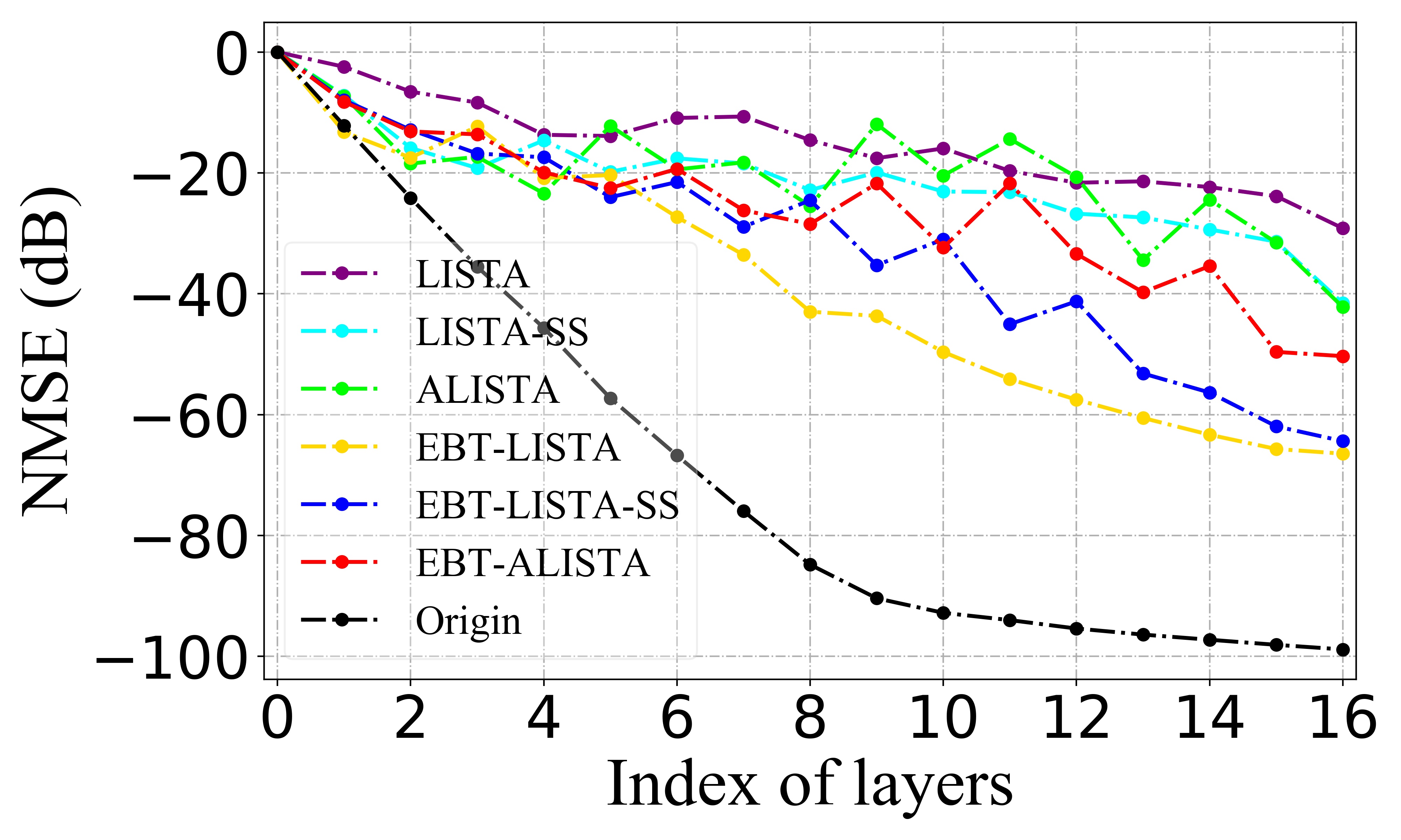
(a) $p_{b}$ changes from 0.8 to 0.99

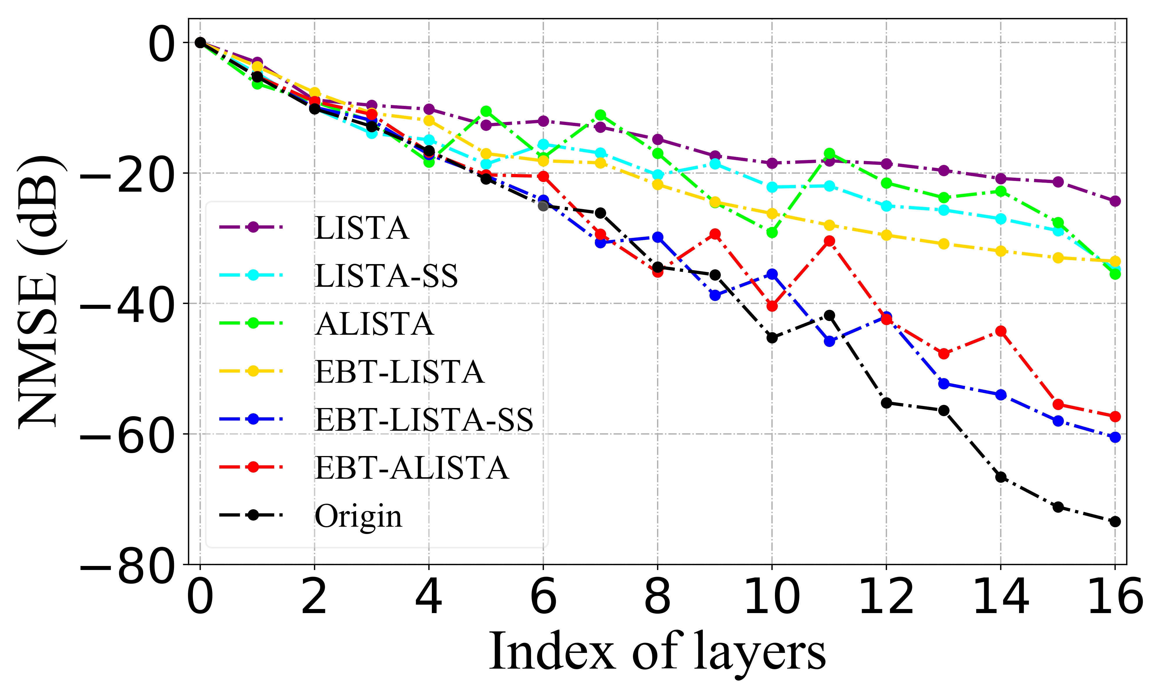
(b) $p_{b}$ changes from 0.8 to 0.9

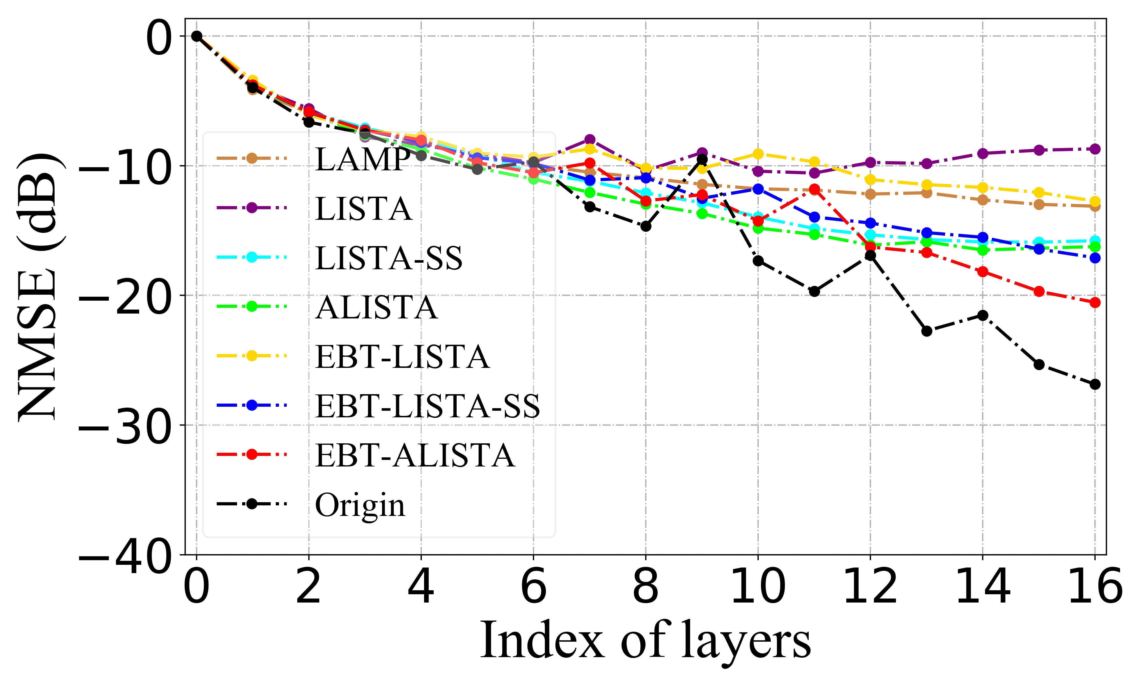
(c) $p_{b}$ changes from 0.9 to 0.8

Fig. 1: NMSE of different models when the test sparsity is different from the training sparsity. We use “Origin” to indicate the optimal scenario where the LISTA models are trained on exactly the same sparsity as that of the test data.

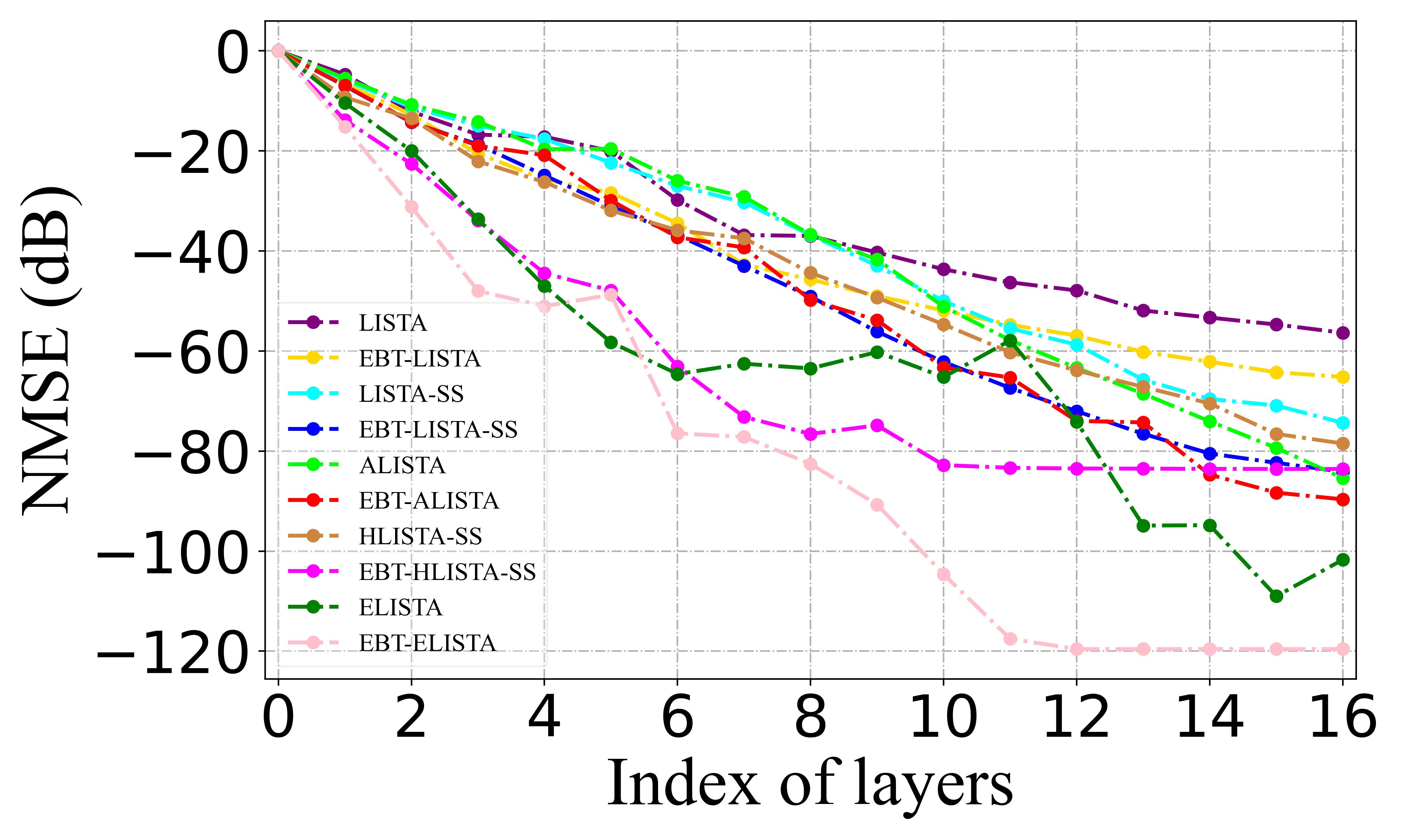
(a) $p_{b}$=0.95

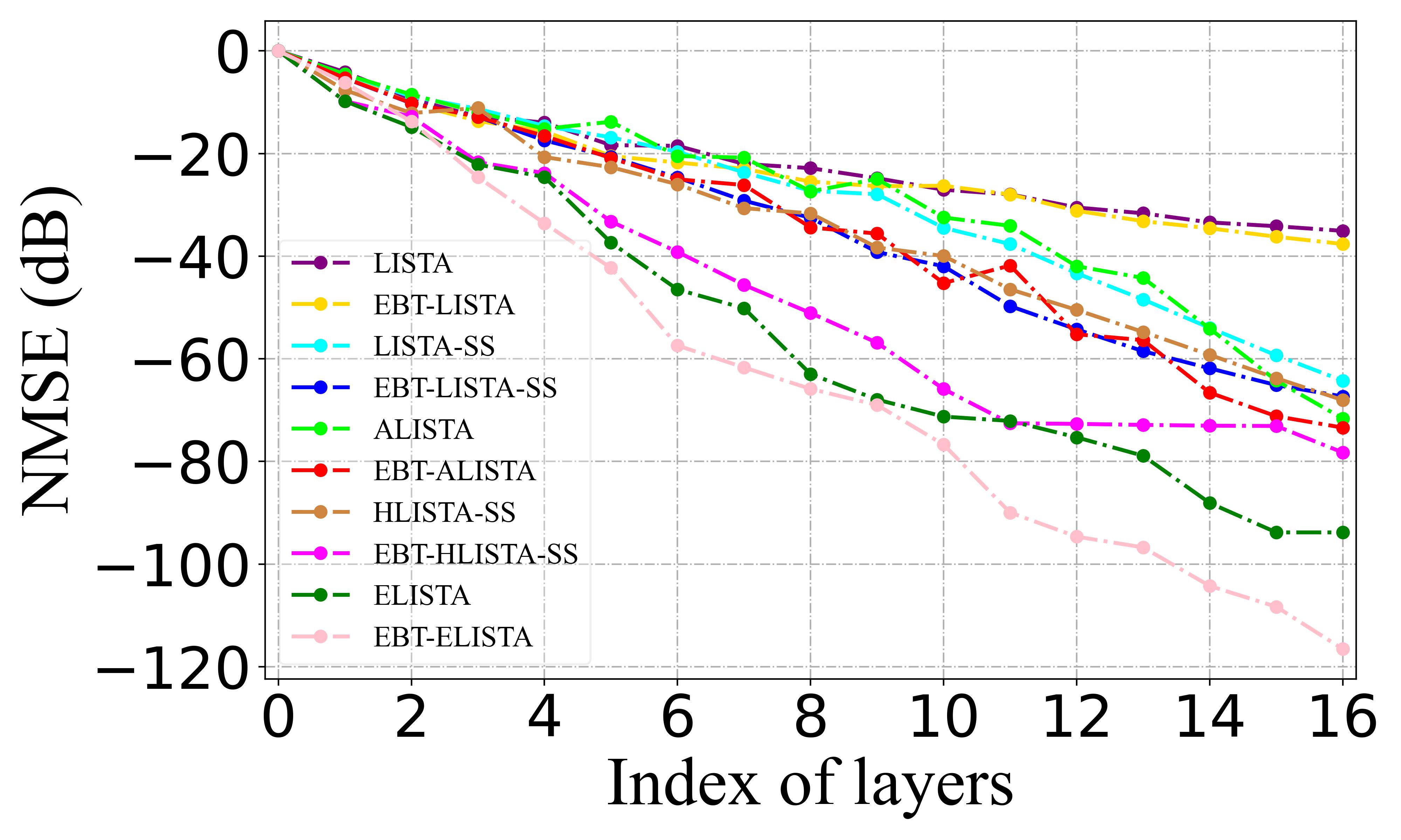
(b) $p_{b}$=0.9

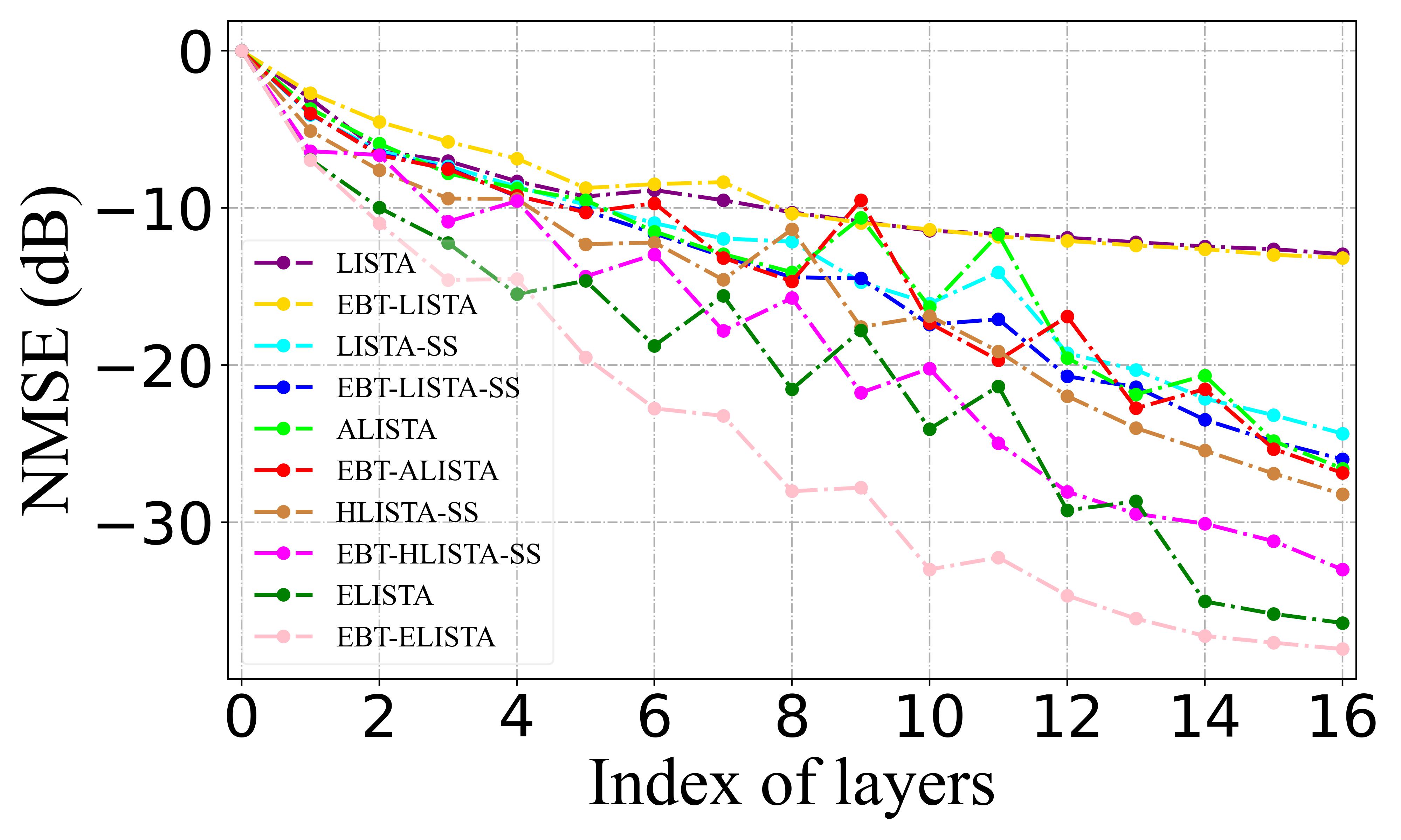
(c) $p_{b}$=0.8

Fig. 2: NMSE of different models under different sparsity. When combined with our EBT, faster convergence is obtained.

5.1 Simulation Experiments

Disentanglement. First, we would like to compare the learned parameters (i.e., $b^{(t)}$ and $\rho^{(t)}$) for the thresholds in both LISTA and our EBT-LISTA. Figure 3a shows how the learned parameters (in a logarithmic coordinate) vary across layers in LISTA and EBT-LISTA. Note that the mean values are removed to align the range of the parameters of different models on the same y-axis. It can be seen that the obtained values for the parameter in EBT-LISTA do not change much from lower layers to higher layers, while the reconstruction errors in fact decrease. By contrast, the obtained threshold values in LISTA vary a lot across layers. Such results imply that the optimal thresholds in EBT-LISTA are indeed independent to (or say disentangled from) the reconstruction error, which well confirms our theoretical result in Theorem 1. Similar observations can also be made on LISTA-SS (i.e., LISTA with support selection) and our EBT-LISTA-SS.

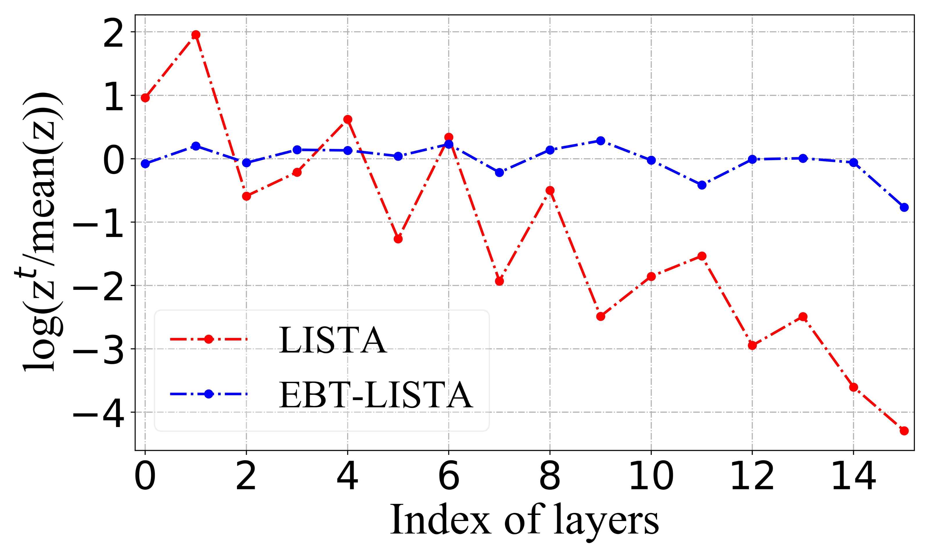
(a) LISTA

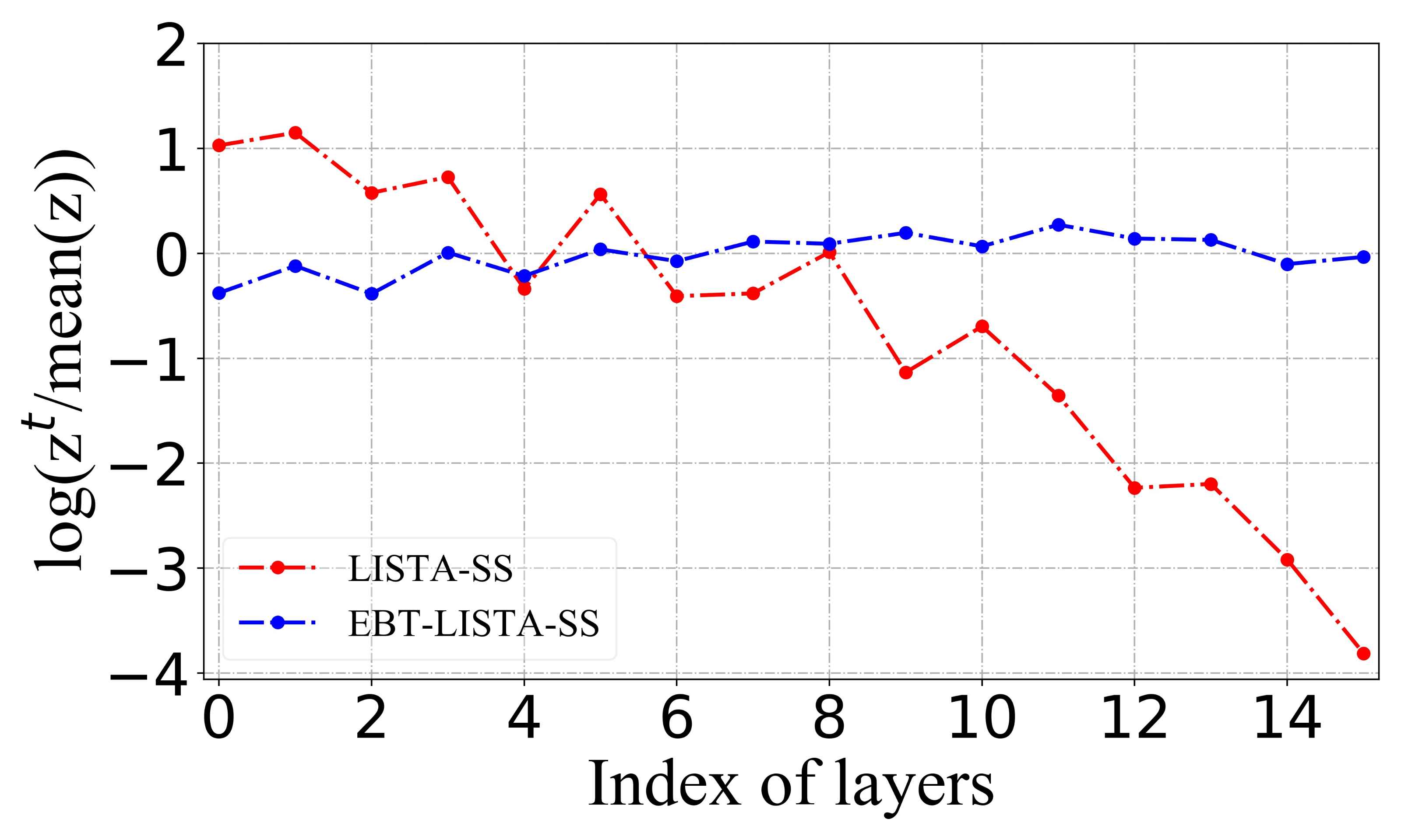
(b) LISTA-SS

Fig. 3: Disentanglement of the reconstruction error and learnable parameters in our EBT. $z^{(t)}$ here indicates $\rho^{(t)}$ and $b^{(t)}$ for networks with or without EBT, respectively.

Adaptivity to unknown sparsity. As have been mentioned, in some practical scenarios, there may exist an obvious gap between the training and test data distribution, or we may not know the distribution of real test data and have to train on synthesized data based on the guess of the test distribution. Under such circumstances, it is of importance to consider the adaptivity/generalization of the sparse coding model (trained on a specific data distribution or with a specific sparsity and the test data sampled from different distributions with different sparsity). To evaluate in such scenario, we let the test sparsity be different from the training sparsity. Figure 2 shows the results in three different test settings (the performance is evaluated by the normalized mean squared error (NMSE) in decibels (dB)). The black curves represent the optimal model when LISTA is trained on exactly the same sparsity as that of the test data. It can be seen that our EBT has huge advantages in such a practical scenario where the adaptivity to un-trained sparsity is required, and the performance gain is larger when the distribution shift between training and test is larger (cf. purple line and yellow line in Figures 1a and 1b).

Combination with other methods. As previously mentioned, our EBT can be combined with many prior efforts (in addition to LISTA, LISTA-SS, and ALISTA). Here we will show its effectiveness with ELISTA [9] and HLISTA with support selection (HLISTA-SS) [10]. For the methods with support selection (i.e., LISTA-SS, EBT-LISTA-SS, ALISTA, EBT-ALISTA, HLISTA-SS,and EBT-HLISTA-SS), we adopt $p=0.6$ and $p_{max}=6.5$ for $p_{b}=0.95$. We let $p$ and $p_{max}$ be 1.2 and 13.0 for $p_{b}=0.9$, and let them be 1.5 and 16.25 for $p_{b}=0.8$. Figure 2 demonstrates some of the results in different sparsity settings, while more results including different noise levels and different condition numbers can be found in the appendices. In all settings, we can see that our EBT leads to significantly faster convergence. In addition, the superiority of our EBT-based models is more significant with a larger $p_{b}$ for which the assumption of $s$ is more likely to hold.

5.2 Photometric Stereo Analysis

We also consider a practical sparse coding task: photometric stereo analysis [11]. The task solves the problem of estimating the normal direction of a Lambertian surface, given $q$ observations under different light directions $L\in\mathbb{R}^{q\times 3}$. Note that the noise is sparse, thus we estimate the noise first, and then calculate the desired normal direction.

Table 1: Mean error (in degree) with different number of observations and different test sparsity.

$p_{e}$	$q$	$l_{1}$	LISTA-SS	EBT-LISTA-SS
	15	0.678	$5.50\times 10^{-2}$	$4.09\times 10^{-2}$
0.8	25	0.408	$7.48\times 10^{-3}$	$3.17\times 10^{-3}$
	35	0.336	$1.89\times 10^{-3}$	$5.95\times 10^{-4}$
	15	0.232	$6.67\times 10^{-3}$	$2.57\times 10^{-3}$
0.9	25	0.145	$1.33\times 10^{-3}$	$1.64\times 10^{-4}$
	35	0.088	$2.93\times 10^{-4}$	$4.91\times 10^{-5}$

In this experiment, we mainly follow the settings in  [12] and  [6]. We use the same bunny picture for evaluation and $L$ is also randomly selected from the hemispherical surface. We set the number of observations $q$ to be $15$, $25$, and $35$, and training sparsity is $p_{t}=0.8$. The final performance is evaluated by calculating the average angle between the estimated normal vector and the ground-truth normal vector (in degree). Since the distribution of the noise is generally unknown in practice, the adaptivity is of greater importance for this task. We use two test settings for evaluating different models, in which the sparsity of the noise in test data (i.e., $p_{e}$) is set as 0.8 and 0.9, respectively. We compare EBT-LISTA-SS, LISTA-SS, and a conventional methods, i.e., least 1-norm ($l_{1}$). Results in Table 1 show that EBT-LISTA-SS outperforms in the concerned settings, which means our EBT-based network can be more effective in this task. Note that the advantage is more remarkable when $p_{e}=0.9$, i.e., $p_{e}\neq p_{t}$, which means EBT-based network has better adaptivity than the original LISTA-based networks.

6 Conclusion

In this paper, we have studied the thresholds in the shrinkage functions of LISTA. We have proposed a novel mechanism called EBT which well disentangles the learnable parameter in the shrinkage function on each layer of LISTA from its layer-wise reconstruction error. We have proved theoretically that, in combination with LISTA or its existing variants, our EBT mechanism leads to faster convergence and achieves superior final sparse coding performance. Also, we have shown that the EBT mechanism endows deep unfolding models with higher adaptivity to different observations with a variety of sparsity. Our experiments on both synthetic data and real data have testified the effectiveness of our EBT, especially when the distributions of the test and training data are different.

References

- [1] Ingrid Daubechies, Michel Defrise, and Christine De Mol, “An iterative thresholding algorithm for linear inverse problems with a sparsity constraint,” Communications on Pure and Applied Mathematics: A Journal Issued by the Courant Institute of Mathematical Sciences, vol. 57, no. 11, pp. 1413–1457, 2004.
- [2] Karol Gregor and Yann LeCun, “Learning fast approximations of sparse coding,” in Proceedings of the 27th International Conference on International Conference on Machine Learning. Omnipress, 2010, pp. 399–406.
- [3] Xiaohan Chen, Jialin Liu, Zhangyang Wang, and Wotao Yin, “Theoretical linear convergence of unfolded ista and its practical weights and thresholds,” in Advances in Neural Information Processing Systems, 2018, pp. 9061–9071.
- [4] Jialin Liu, Xiaohan Chen, Zhangyang Wang, and Wotao Yin, “Alista: Analytic weights are as good as learned weights in lista,” in International Conference on Learning Representations (ICLR), 2019.
- [5] Pierre Ablin, Thomas Moreau, Mathurin Massias, and Alexandre Gramfort, “Learning step sizes for unfolded sparse coding,” in Advances in Neural Information Processing Systems, 2019, pp. 13100–13110.
- [6] Kailun Wu, Yiwen Guo, Ziang Li, and Changshui Zhang, “Sparse coding with gated learned ista,” in Proceedings of the International Conference on Learning Representations, 2020.
- [7] Aviad Aberdam, Alona Golts, and Michael Elad, “Ada-lista: Learned solvers adaptive to varying models,” IEEE Transactions on Pattern Analysis and Machine Intelligence, 2021.
- [8] Joey Tianyi Zhou, Kai Di, Jiawei Du, Xi Peng, Hao Yang, Sinno Jialin Pan, Ivor W Tsang, Yong Liu, Zheng Qin, and Rick Siow Mong Goh, “Sc2net: Sparse lstms for sparse coding,” in Thirty-Second AAAI Conference on Artificial Intelligence, 2018.
- [9] Yangyang Li, Lin Kong, Fanhua Shang, Yuanyuan Liu, Hongying Liu, and Zhouchen Lin, “Learned extragradient ista with interpretable residual structures for sparse coding,” in Proceedings of the AAAI Conference on Artificial Intelligence, 2021, vol. 35, pp. 8501–8509.
- [10] Ziyang Zheng, Wenrui Dai, Duoduo Xue, Chenglin Li, Junni Zou, and Hongkai Xiong, “Hybrid ista: unfolding ista with convergence guarantees using free-form deep neural networks,” IEEE Transactions on Pattern Analysis and Machine Intelligence, 2022.
- [11] Satoshi Ikehata, David Wipf, Yasuyuki Matsushita, and Kiyoharu Aizawa, “Robust photometric stereo using sparse regression,” in 2012 IEEE Conference on Computer Vision and Pattern Recognition. IEEE, 2012, pp. 318–325.
- [12] Bo Xin, Yizhou Wang, Wen Gao, David Wipf, and Baoyuan Wang, “Maximal sparsity with deep networks?,” in Advances in Neural Information Processing Systems, 2016, pp. 4340–4348.