RIKEN-iTHEMS-Report-21,

Analytic Bootstrap in 2D Boundary Conformal Field Theory:
Towards Braneworld Holography
Yuya Kusuki ^1,2

¹Walter Burke Institute for Theoretical Physics
California Institute of Technology, Pasadena, CA 91125, USA

²RIKEN Interdisciplinary Theoretical and Mathematical Sciences (iTHEMS),
Saitama 351-0198, Japan

Recently, boundary conformal field theories (BCFTs) have attracted much attention in the context of quantum gravity. This is because a BCFT can be dual to gravity coupled to a heat bath CFT, known as the island model. On this background, it would be interesting to explore the duality between the boundary and the braneworld. However, this seems to be a challenging problem. The reason is because although there has been much study of rational BCFTs, there has been comparatively little study of irrational BCFTs, and irrational BCFTs are expected to be the boundary duals of the braneworlds. For this reason, we explore properties of boundary ingredients: the boundary primary spectrum, the boundary-boundary-boundary OPE coefficients and the bulk-boundary OPE coefficients. For this purpose, the conformal bootstrap is extremely useful. This is the first step in providing an understanding of BCFTs in the context of braneworld holography by using the conformal bootstrap. The techniques developed in this paper may be useful for further investigation of irrational BCFTs.

1 Introduction & Summary

1.1 Introduction

Recently, there has been tremendous progress on the information paradox problem. The idea is to consider a setup where a CFT_d on AdS_d and a CFT_d on a non-gravitational bath are glued along the (asymptotic) boundary [1, 2, 3]. Since light can go through the asymptotic boundary in this setup, we can probe the Hawking radiation from black holes by the entanglement entropy between the gravitational and bath systems. This setup is sometimes called “doubly holography”. This is because we have three pictures, which are equivalent (see Figure 1). By applying the AdS/CFT correspondence [4] to the AdS_d gravity in this setup (left of Figure 1), we can obtain a boundary conformal field theory, where the boundary is dual to the AdS_d gravity (right of Figure 1 ). We can obtain another picture by applying the AdS/BCFT correspondence [5, 6] to this BCFT (see bottom of Figure 1). Here we apply the AdS/CFT correspondence “twice”, so we call this holography the doubly holography. The bottom picture in Figure 1 is sometimes useful because we can evaluate “quantum” entanglement therein by just calculating the holographic entanglement entropy (i.e. the area of Ryu-Takayanagi surface) in the setup shown in bottom of Figure 1 (for example, see [7, 8, 9, 10, 11, 12, 13, 14, 15, 16]).

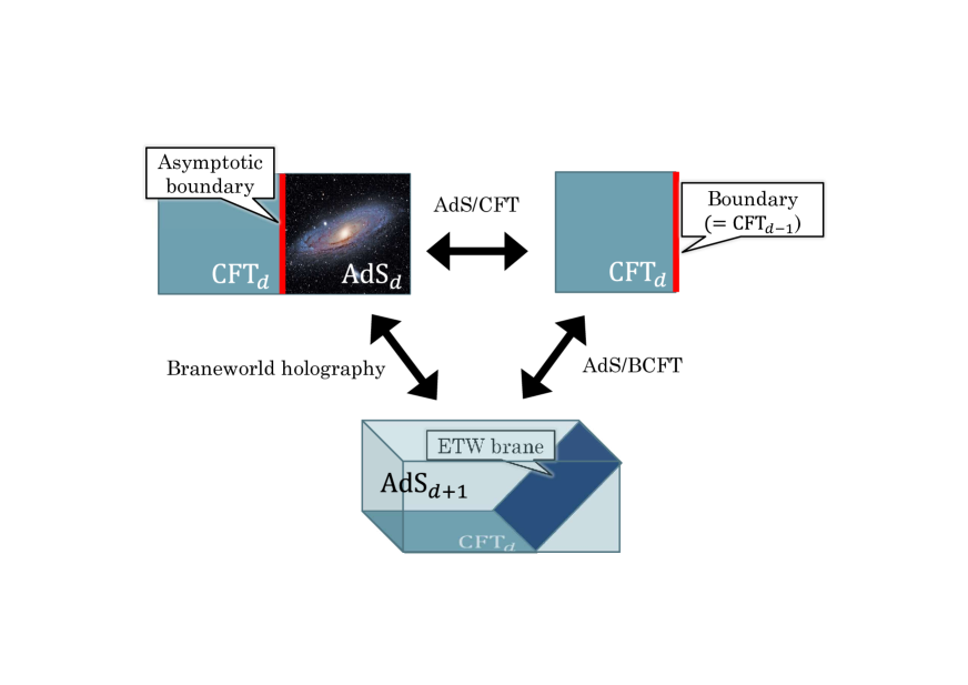
Figure 1: Triality through the AdS/CFT correspondence. The CFT drawn in the left is dual to the BCFT drawn in the right through the AdS/CFT correspondence. Moreover, the BCFT is dual to the quantum gravity shown at the bottom through the AdS/BCFT correspondence. There is also a relation between the left picture and the bottom picture through the braneworld holography [17, 18, 19].

On this background, it would be very interesting to explore the duality,

$d$ dimensional boundary of CFT_d+1 = $d+1$ dimensional braneworld

In particular, it would be interesting to consider the question, “can the boundary be dual to classical gravity?” or “which type of gravity is realized on the braneworld associated with the BCFT?”. Nevertheless, there has been little knowledge of the CFT with this holographic boundary. This is because there has been currently very little knowledge of irrational BCFTs. For example, many techniques in CFTs with no boundaries have been generalized to CFTs with boundaries, and various constraints have been given by using the conformal bootstrap equation as shown in [24]. However, these results are given only when we restrict ourselves to rational conformal field theories (RCFTs).

Against this backdrop, it is very important to exhibit various universal formulae in irrational CFTs with boundaries. For example, the universal formula for the entropy at high energy, known as the Cardy formula [25], plays an important role in the understanding of quantum gravity. This entropy formula surprisingly matches with the black hole entropy [26]. This result may therefore answer the greatest question, “Is black hole thermodynamics is really thermodynamics?”. The Cardy formula answers this question, “Yes”. This accomplishment surely supports the high usefulness of discovering universal formulae in BCFTs with some assumptions that are needed for reproducing classical gravity.

There is a useful tool to identify unknown information in a given CFT, known as the conformal bootstrap. The conformal bootstrap is just a consistency condition in CFTs, more precisely, the OPE associativity. We can utilize this consistency condition to give non-trivial constraints on the spectrum and the OPE coefficients in a given CFT. Some significant breakthroughs have been achieved by the numerical application (or the low-order approximation inspired by that) of the conformal bootstrap to investigate low-lying operators [27, 28, 29, 30, 31], the upper bound on the gap from the vacuum [32, 33, 31, 34, 35, 36] and the uniqueness of Liouville CFT [37]. The conformal bootstrap equation can also be used to derive universal formulae in some asymptotic regions. For example, one can derive the universal formula for the spectrum at high energy region [25, 38, 39], the heavy-light-light OPE coefficients [40, 41, 42, 43, 44], the heavy-heavy-light OPE coefficients [45, 46, 47, 48], the heavy-heavy-heavy OPE coefficients [49] and the OPE in the large spin limit [50, 51, 52, 53, 54, 55, 56, 57, 58, 59].

Recently, there is remarkable progress in solving the bootstrap equation in 2D CFTs. The idea is to act the fusion transformation on the vacuum block, which provides a new analytic method to access the CFT data. The fusion matrix bootstrap has provided important progress in the light cone conformal bootstrap [60, 31, 61] and the light-cone modular bootstrap [62, 63, 64]. Moreover, by making use of the fusion matrix bootstrap, all of the results in [40, 41, 42, 43, 45, 46, 47, 48, 49] can be organized [65, 66, 67]. For this reason, in this article, we investigate universal formulae in BCFTs by using the fusion matrix bootstrap.

1.2 Summary

One goal of this paper is to formulate the bootstrap equation in irrational BCFTs and to clarify what we can learn from the bootstrap equation beyond rational BCFTs. The techniques developed in this paper are very useful to provide a new understanding of the braneworld holography from the CFT side. Although we only show the asymptotic universal formulae in this paper, there are a lot of applications of our techniques in the context of the braneworld holography. At the end of this paper, we propose some interesting questions that we can address by using our techniques.

Here we briefly summarize our results:

• Universality for OPE coefficients (Section 4)

  The asymptotic behaviors of the OPE coefficients can be estimated by using the fusion matrix bootstrap. In particular, we will show the universal formulae for

  • boundary primary spectrum (i.e., open-string spectrum) at high energy,

  • boundary-boundary-boundary OPE coefficients for heavy-heavy-heavy weights,

  • boundary-boundary-boundary OPE coefficients for heavy-heavy-light weights,

  • boundary-boundary-boundary OPE coefficients for heavy-light-light weights,

  • bulk-boundary OPE coefficients for heavy-heavy weights,

  • bulk-boundary OPE coefficients for heavy-light weights,

  • bulk-boundary OPE coefficients for light-heavy weights.

  For this purpose, we will consider various bootstrap equations on various manifolds. Although in principle, we can fix all components in a BCFT by considering only six conformal bootstrap equations [68], it is useful to consider other bootstrap equations to fix the asymptotics in practice.

• Light-cone bootstrap in BCFT (Section 5)

  We will show that in some setups, we can consider the large-spin asymptotics of the OPE coefficients even though BCFTs do not have the anti-holomorphic part. It implies that it would be possible to consider an analog of the light-cone modular bootstrap [63] in BCFTs.

• Braneworld holography (Section 6)

  Although many recent works heavily make use of the braneworld holography, there is very limited knowledge about this type of holography. We believe that the braneworld should be realized on the boundary of the BCFT, nevertheless, we do not know what gravity is realized as the boundary of the BCFT. Some hints can be obtained from the asymptotics of the boundary ingredients, like the matching between the Cardy formula and the Bekenstein-Hawking entropy. In some recent works, we consider the braneworld in the JT or Liouville gravity, which can have black hole solutions. From this observation, we can expect that the boundary ingredients follow the Cardy formula, the eigenstate thermalization hypothesis (ETH), and some other chaotic nature, like the AdS₃ gravity. On this background, we will give some thoughts on the braneworld. Here we do not give the explicit connection between the braneworld and the BCFT because our main purpose is to give a new tool to access the data of the boundary ingredients in irrational BCFTs as the first step. We hope that we will show the explicit connection by using our results obtained here in the near future paper.

Note that some of our results can also be straightforwardly applied to the one-dimensional conformal bootstrap. This consideration could provide a generalization of the analytic bootstrap result in 1D CFT [69, 70] into a Virasoro version. For example, our result (4.35) can be thought of as the Virasoro generalization of the asymptotic results in [69, 70]. On the bulk side, the Virasoro generalization allows us to access information including graviton effects. This is particularly useful to consider the black hole information paradox as one can see in [59, 71, 72] since the exchange of the Virasoro descendants can create an effect of the presence of the BTZ black hole background, unlike the global conformal descendants.

2 Review of Fusion Matrix Bootstrap

In this section, we will review how to solve the conformal bootstrap equation by using the fusion matrix, first introduced in [60, 61, 73] and generalized in [66].

The conformal bootstrap equation is the relation between different OPE coefficients $C_{ijk}$ in the following form,

$$\sum_{p}C_{12p}C_{34p}\mathcal{F}^{21}_{34}(h_{p}|z)\overline{\mathcal{F}^{21}_{34}}(\bar{h}_{p}|\bar{z})$$ (2.1)

$$=\sum_{p}C_{14p}C_{23p}\mathcal{F}^{23}_{14}(h_{p}|1-z)\overline{\mathcal{F}^{23}_{14}}(\bar{h}_{p}|1-\bar{z}),$$

where we define the Virasoro conformal block as follows,

$$\mathcal{F}^{ji}_{kl}(h_{p}|z)\equiv\parbox{119.9682pt}{\leavevmode\hbox{\includegraphics[width=120.0pt]{ijkl.pdf}}}.$$ (2.2)

For simplicity, we focus on the case where $h_{1}=h_{2}=h_{A}$ and $h_{3}=h_{4}=h_{B}$. Even though it is hard to solve this equation in general, in some asymptotic regimes, we can analytically solve the bootstrap equation. Here, we will show some examples. In the limit as $z,\bar{z}\to 0$, we can approximate the bootstrap equation as

$$\mathcal{F}^{AA}_{BB}(0|z)\overline{\mathcal{F}^{AA}_{BB}}(0|\bar{z})\simeq\sum_{p}C_{ABp}C_{ABp}\mathcal{F}^{AB}_{AB}(h_{p}|1-z)\overline{\mathcal{F}^{AB}_{AB}}(\bar{h}_{p}|1-\bar{z}),$$ (2.3)

The key point is that we have invertible fusion transformations between the s and t-channel Virasoro conformal block.

$$\mathcal{F}^{AA}_{BB}(0|z)$$ (2.4)

$$=\sum_{\begin{subarray}{c}{\alpha}_{n,m}<\frac{Q}{2}\\ n,m\in\mathbb{Z}_{\geq 0}\end{subarray}}\ \text{Res}\left(-2\pi i{\mathbb{F}}_{0,{\alpha}_{t}}\left[\begin{array}[]{cc}{\alpha}_{A}&{\alpha}_{A}\\ {\alpha}_{B}&{\alpha}_{B}\\ \end{array}\right]\mathcal{F}^{AB}_{AB}(h_{t}|1-z);{\alpha}_{t}={\alpha}_{n,m}\right)$$

$$+\int_{\frac{Q}{2}+0}^{\frac{Q}{2}+i\infty}{\mathrm{d}}{\alpha}_{t}{\mathbb{F}}_{0,{\alpha}_{t}}\left[\begin{array}[]{cc}{\alpha}_{A}&{\alpha}_{A}\\ {\alpha}_{B}&{\alpha}_{B}\\ \end{array}\right]\mathcal{F}^{AB}_{AB}(h_{t}|1-z),$$

where ${\alpha}_{n,m}\equiv{\alpha}_{A}+{\alpha}_{B}+mb+nb^{-1}$ and kernel ${\mathbb{F}}_{{\alpha}_{s},{\alpha}_{t}}$ denotes the fusion matrix (or crossing matrix), and we introduce the notation usually found in the Liouville CFT,

$$c=1+6Q^{2},\ \ \ \ \ Q=b+\frac{1}{b},\ \ \ \ \ h_{i}={\alpha}_{i}(Q-{\alpha}_{i}),\ \ \ \ \ \bar{h}_{i}=\bar{{\alpha}}_{i}(Q-\bar{{\alpha}}_{i}).$$ (2.5)

For simplicity, we define the degeneracy of primary states $\rho({\alpha},\bar{{\alpha}})$ as

$$\rho({\alpha},\bar{{\alpha}})=\sum_{p}D_{p}\delta({\alpha}-{\alpha}_{p})\delta(\bar{{\alpha}}-\bar{{\alpha}}_{p}),$$ (2.6)

where the function $D_{p}$ denotes the degeneracy of primary operators with weights $(h_{p},\bar{h}_{p})$ and then define the averaged OPE coefficients as

$$\rho(\alpha_{p},\bar{\alpha}_{p})\overline{C_{ABp}C_{ABp}}=\sum_{q}C_{ABq}C_{ABq}\delta\left(\alpha_{p}-\alpha_{q}\right)\delta\left(\bar{\alpha}_{p}-\bar{\alpha}_{q}\right),$$ (2.7)

where the average is taken over the states with the Liouville momentum $({\alpha}_{p},\bar{{\alpha}}_{p})$.

With this notation, we obtain the following asymptotic bootstrap equation,

$$\int{\mathrm{d}}{\alpha}_{p}{\mathrm{d}}\bar{{\alpha}}_{p}\ {\mathbb{F}}_{0,{\alpha}_{p}}\left[\begin{array}[]{cc}{\alpha}_{A}&{\alpha}_{A}\\ {\alpha}_{B}&{\alpha}_{B}\\ \end{array}\right]{\mathbb{F}}_{0,\bar{{\alpha}}_{p}}\left[\begin{array}[]{cc}\bar{{\alpha}}_{A}&\bar{{\alpha}}_{A}\\ \bar{{\alpha}}_{B}&\bar{{\alpha}}_{B}\\ \end{array}\right]\mathcal{F}^{AB}_{AB}(h_{p}|1-z)\overline{\mathcal{F}^{AB}_{AB}}(\bar{h}_{p}|1-\bar{z})$$ (2.8)

$$\simeq\int{\mathrm{d}}{\alpha}_{p}{\mathrm{d}}\bar{{\alpha}}_{p}\ \rho(\alpha_{p},\bar{\alpha}_{p})\overline{C_{ABp}C_{ABp}}\mathcal{F}^{AB}_{AB}(h_{p}|1-z)\overline{\mathcal{F}^{AB}_{AB}}(\bar{h}_{p}|1-\bar{z}).$$

Thus, we can find the universal asymptotic formula for the OPE coefficients as

$$\rho(\alpha_{p},\bar{\alpha}_{p})\overline{C_{ABp}C_{ABp}}\simeq{\mathbb{F}}_{0,{\alpha}_{p}}\left[\begin{array}[]{cc}{\alpha}_{A}&{\alpha}_{A}\\ {\alpha}_{B}&{\alpha}_{B}\\ \end{array}\right]{\mathbb{F}}_{0,\bar{{\alpha}}_{p}}\left[\begin{array}[]{cc}\bar{{\alpha}}_{A}&\bar{{\alpha}}_{A}\\ \bar{{\alpha}}_{B}&\bar{{\alpha}}_{B}\\ \end{array}\right],\ \ \ \ \ \ \ h_{p},\bar{h}_{p}\to\infty.$$ (2.9)

The explicit form of the fusion matrix is given in Appendix A. In particular, the asymptotic behavior of the fusion matrix is given by

$${\mathbb{F}}_{0,{\alpha}_{p}}\left[\begin{array}[]{cc}{\alpha}_{A}&{\alpha}_{A}\\ {\alpha}_{B}&{\alpha}_{B}\\ \end{array}\right]\simeq 16^{-h_{p}}\mathrm{e}^{\pi\sqrt{\frac{c}{6}\left(h_{p}-\frac{c}{24}\right)}}\ \ \ \ \ \ \ h_{p}\to\infty.$$ (2.10)

This asymptotic behavior is consistent with the results in [40, 41, 42, 43], which derive the asymptotic behavior of the OPE coefficients in a different way, using the inverse Laplace transformation. Note that the above result (2.9) should be interpreted as the density of states averaged over a small window. The dependence on the size of the window can be obtained by using the Tauberian theorem [88, 43], which show that a change of the size only gives $O(1)$ corrections. In this paper, we will not attempt here to care about the size of the window. It would be interesting to applying the Tauberian theorem on our results in a similar way as [88, 43].

The same approach can also be applied to the modular bootstrap equation. The partition function can be expressed by

$$Z(\tau,\bar{\tau})=\int{\mathrm{d}}{\alpha}_{p}{\mathrm{d}}\bar{{\alpha}}_{p}\ \rho({\alpha}_{p},\bar{{\alpha}}_{p})\chi_{h_{p}}(\tau)\bar{\chi}_{\bar{h}_{p}}(\bar{\tau}),$$ (2.11)

where $\chi_{h_{p}}(\tau)$ is the Virasoro character. The character has an analog of the fusion transformation, so-called the modular-S transformation,

$$\chi_{h_{p}}(\tau)=\int{\mathrm{d}}{\alpha}_{q}\ S_{pq}\chi_{h_{q}}\left(-\frac{1}{\tau}\right).$$ (2.12)

Thus, in the same way as the conformal bootstrap, we obtain the universal asymptotic formula for the density of states as

$$\rho({\alpha}_{p},\bar{{\alpha}}_{p})\simeq S_{0p}\bar{S}_{0p},\ \ \ \ \ \ \ h_{p},\bar{h}_{p}\to\infty.$$ (2.13)

Note that the explicit form of the modular-S matrix is given by

$$S_{0p}=-4\sqrt{2}\sin\left(2\pi b\left({\alpha}-\frac{Q}{2}\right)\right)\sin\left(2\pi\frac{1}{b}\left({\alpha}-\frac{Q}{2}\right)\right).$$ (2.14)

The asymptotic behavior of the modular-S matrix is

$$S_{0p}\simeq\mathrm{e}^{2\pi\sqrt{\frac{c}{6}\left(h_{p}-\frac{c}{24}\right)}},\ \ \ \ \ \ \ h_{p}\to\infty.$$ (2.15)

This completely matches the Cardy formula. In other words, the result (2.13) is just another derivation of the Cardy formula.

3 Boundary Conformal Field Theory

Let us move on to conformal field theories with boundaries. As shown in [24], if we restrict ourselves to boundary conditions satisfying

$$\left.T(z)=\bar{T}(\bar{z})\right|_{\text{bdy}},$$ (3.1)

we can directly relate the analytic structure of correlators on the upper half plane to that on the full plane. More precisely, we can reconstruct the Ward identity if we consider $\bar{T}(\bar{z})$ to be the analytic continuation of $T(z)$ into the lower half plane. It means that the Virasoro algebra can fix many ingredients in BCFTs, like in CFTs without boundaries as we have seen in Section 2.

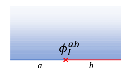
Figure 2: The definition of the boundary operator. The index $I$ labels a primary field with the conformal dimension $h_{I}$ and the indices $a,b$ denote its boundary conditions, where the boundary condition $a$ is changed to $b$ by the operator $\phi^{ab}_{I}$.

Let us consider what the new ingredients are, other than the bulk ingredients, In addition to bulk primary operators $\phi_{i}$, BCFTs have boundary primary operators $\phi^{ab}_{I}(x)$, which live only on the boundary (see Figure 2). The index $I$ labels a primary field with the conformal dimension $h_{I}$ and the indices $a,b$ denote its boundary conditions, where the boundary condition $a$ is changed to $b$ by the operator $\phi^{ab}_{I}(x)$. In the following, we denote the bulk primary operators by $\phi$ with lowercase letters $i$ and the boundary primary operators by $\phi$ with capital letter $I$.

The dynamics of a BCFT can be completely determined by the following information,

Disk partition function (i.e., boundary entropy)

$$\braket{\mathbb{I}}_{a}=g^{a},$$ (3.2)

Boundary-boundary-boundary OPE coefficients

$$\phi^{ab}_{I}(0)\phi^{bc}_{J}(x)\sim\sum_{K}C^{abc}_{IJK}x^{h_{K}-h_{I}-h_{J}}\phi^{ac}_{K}(x)+\cdots,$$ (3.3)

Bulk-boundary OPE coefficients

$$\phi_{i}(z)\sim\sum_{I}(2\Im z)^{h_{I}-h_{i}-\bar{h}_{i}}C^{a}_{iI}\phi^{aa}_{I}(\Re z)+\cdots,$$ (3.4)

Bulk-bulk-bulk OPE coefficients

$$\phi_{i}(0)\phi_{j}(z)\sim\sum_{k}C_{ijk}z^{h_{k}-h_{i}-h_{j}}\bar{z}^{\bar{h}_{k}-\bar{h}_{i}-\bar{h}_{j}}\phi_{k}(z)+\cdots.$$ (3.5)

Note that the normalization $g^{a}$ in (3.2) cannot be freely chosen. Let us consider an RCFT to see this explicitly. From eq.(3.1), one can show that possible boundary conditions can be expressed in terms of the Ishibashi states,

$$\ket{j}\rangle\equiv\sum_{N}\ket{j;N}\otimes U\overline{\ket{j;N}},$$ (3.6)

where $\ket{j;N}$ is a state in the Verma module $j$ labeled by $N$, and $U$ is an anti-unitary operator. Moreover, the open-closed duality constraints the possible linear combinations of the Ishibashi states as

$$\ket{\tilde{i}}=\sum_{j}\frac{S_{ij}}{\sqrt{S_{0j}}}\ket{j}\rangle,$$ (3.7)

known as the Cardy state. From this expression , we can immediately find that the disk partition function is given by

$$\braket{\mathbb{I}}_{a}=g^{a}=\frac{S_{a0}}{\sqrt{S_{00}}}.$$ (3.8)

In a similar way, we can also fix the bulk-boundary OPE coefficients with the vacuum boundary operator as [75]

$$C^{a}_{i\mathbb{I}}=\frac{S_{ai}\sqrt{S_{00}}}{S_{a0}\sqrt{S_{0i}}}$$ (3.9)

Our interest is the asymptotic formula for the boundary ingredients where the boundary condition does not matter since the universal feature is only fixed by the Virasoro symmetry (i.e., the properties of Virasoro blocks with no boundary). Therefore, we only focus on a special case where all boundary conditions are the same (i.e., identical boundaries), for simplicity. In the following, we also omit the index $a$ that specifies the boundary condition to avoid cumbersome expressions.

Let us consider a natural normalization for a two point function,

$$\braket{\phi_{I}(0)\phi_{J}(x)}=\delta_{IJ}x^{-2h_{I}}{\alpha}_{I}.$$ (3.10)

Naively, we could set ${\alpha}_{I}$ freely by suitable normalization of the boundary primary fields $\phi_{I}$. However, we have the non-trivial normalization for the vacuum amplitude, $g$, which leads to a natural normalization ${\alpha}_{I}=g$. Note that, for example in [75], the normalization is set to be ${\alpha}_{I}=1$. In this case, one can find that $C_{\mathbb{I}\mathbb{I}}\neq 1$, which seems to be unnatural. For this reason, we set ${\alpha}_{I}=g$ in the following. With this normalization, we have

$$C_{\mathbb{I}\mathbb{I}}=1,$$ (3.11)

$$C_{\mathbb{I}II}=1,$$ (3.12)

Now we have four simplified components in a BCFT,

Disk partition function(i.e., boundary entropy)

$$\parbox{59.9841pt}{\leavevmode\hbox{\includegraphics[width=60.0pt]{disk.pdf}}}\equiv g.$$ (3.13)

Boundary-boundary-boundary OPE coefficients

$$\parbox{59.9841pt}{\leavevmode\hbox{\includegraphics[width=60.0pt]{bdy3pt.pdf}}}\equiv C_{IJK}.$$ (3.14)

Bulk-boundary OPE coefficients

$$\parbox{59.9841pt}{\leavevmode\hbox{\includegraphics[width=60.0pt]{bulkbdy.pdf}}}\equiv C_{iI}.$$ (3.15)

Bulk-bulk-bulk OPE coefficients

$$\parbox{59.9841pt}{\leavevmode\hbox{\includegraphics[width=60.0pt]{bulk3pt.pdf}}}\equiv C_{ijk}.$$ (3.16)

We sketch a sphere without boundaries by a gradient color disk (3.16).

With this information, we can completely evaluate any correlation function. For example, let us consider a two point function on a disk.

This can be decomposed into two parts by inserting the bulk identity $\sum_{p}\ket{p}\bra{p}$ along the red line in the following picture,

Thus, we obtain

$$\parbox{149.5989pt}{\leavevmode\hbox{\includegraphics[width=150.0pt]{ex1-3.pdf}}}=g\sum_{p}C_{p\mathbb{I}}C_{ijp}\parbox{119.9682pt}{\leavevmode\hbox{\includegraphics[width=120.0pt]{ijji.pdf}}},$$ (3.17)

where the diagram is the same as the standard Virasoro conformal block. The prefactor $g$ comes from the bulk-boundary OPE,

$$\braket{\phi_{p}}_{\text{disk}}=\sum_{Q}C_{pQ}\braket{\phi_{Q}}=g\ C_{p\mathbb{I}}.$$ (3.18)

We can obtain another channel expansion by inserting the boundary identity $\frac{1}{g}\sum_{P}\ket{P}\bra{P}$ along the red line in the following picture, where the prefactor $\frac{1}{g}$ comes from the normalization of the boundary two-point function $\braket{P}{P}=g$.

Thus, we obtain

$$\parbox{199.4652pt}{\leavevmode\hbox{\includegraphics[width=200.0pt]{ex2-2.pdf}}}=g\sum_{P}C_{iP}C_{jP}\parbox{119.9682pt}{\leavevmode\hbox{\includegraphics[width=120.0pt]{two-b.pdf}}}.$$ (3.19)

What we would like to emphasize here is that the sewing and cutting procedure in the full plane [76, 77, 78, 79] also work in the upper half-plane. More details can be found in the reference [68]. The point is that any correlation function in a BCFT can also be decomposed in terms of the standard Virasoro block. Therefore, in a similar way as the procedure shown in Section 2, the information about the boundary ingredients at asymptotically large dimensions can be fixed by the fusion matrix. We will show them in the next section.

4 Bootstrap in BCFT

In this section, we will solve various bootstrap equations in a BCFT. In the following, we assume our CFT to be a unitary compact CFT with $c>1$.

4.1 Zero-point on a cylinder: spectrum of boundary primaries

For a zero-point function on a cylinder, we have the following two choices of how to cut,

$$\parbox{70.1019pt}{\leavevmode\hbox{\includegraphics[width=70.0pt]{1-1.pdf}}}=\parbox{70.1019pt}{\leavevmode\hbox{\includegraphics[width=70.0pt]{1-2.pdf}}}.$$ (4.1)

The corresponding bootstrap equation is given by

$$\int{\mathrm{d}}{\alpha}_{P}\ \rho({\alpha}_{P})\parbox{59.9841pt}{\leavevmode\hbox{\includegraphics[width=60.0pt]{torus1.pdf}}}=g^{2}\int{\mathrm{d}}{\alpha}_{p}\ \rho({\alpha}_{p})\overline{C_{p\mathbb{I}}C_{p\mathbb{I}}}\parbox{59.9841pt}{\leavevmode\hbox{\includegraphics[width=60.0pt]{torus2.pdf}}},$$ (4.2)

where the diagram represents the Virasoro character $\chi_{p}(\tau)$ (which depends only on the conformal dimension $h_{p}$ and independent of whether the field lives on the boundary or the bulk), and $\rho({\alpha}_{P})$ represents the density of the “boundary” primary states, which is different from the density of the “bulk” primary states $\rho({\alpha}_{p})\equiv\rho({\alpha}_{p},{\alpha}_{p})$ with lowercase letters. The right hand side can be approximated by the vacuum block if we take the $\tau\to i0$ limit. As a result, we obtain

$$\int{\mathrm{d}}{\alpha}_{P}\ \rho({\alpha}_{P})\parbox{59.9841pt}{\leavevmode\hbox{\includegraphics[width=60.0pt]{torus1.pdf}}} \simeq g^{2}\parbox{59.9841pt}{\leavevmode\hbox{\includegraphics[width=60.0pt]{torus3.pdf}}}$$ (4.3)

$$=g^{2}\int{\mathrm{d}}{\alpha}_{P}\ S_{0P}\parbox{59.9841pt}{\leavevmode\hbox{\includegraphics[width=60.0pt]{torus1.pdf}}}.$$

In the second equation, we use the modular-S transformation (2.12). Thus, the universal formula for the density of the boundary primary states is given by

$$\rho({\alpha}_{P})\simeq g^{2}S_{0P},\ \ \ \ \ \ h_{P}\to\infty.$$ (4.4)

This is similar to the Cardy formula for the spectrum of bulk primaries. Indeed, the same result was derived in [46] by the traditional approach using the inversion Laplace transformation. Note that although we retain the non-universal factor $g$, this factor is subleading in the large $h_{p}$ asymptotics. This is just a constant in the conformal dimension $h_{p}$.

One can take another limit $\tau\to i\infty$, where the left hand side can be approximated by the vacuum block. In a similar way as (4.3), we obtain

$$g^{2}\int{\mathrm{d}}{\alpha}_{p}\ \rho({\alpha}_{p})\overline{C_{p\mathbb{I}}C_{p\mathbb{I}}}\parbox{59.9841pt}{\leavevmode\hbox{\includegraphics[width=60.0pt]{torus2.pdf}}} \simeq\int{\mathrm{d}}{\alpha}_{p}\ S_{0p}\parbox{59.9841pt}{\leavevmode\hbox{\includegraphics[width=60.0pt]{torus2.pdf}}}.$$ (4.5)

This equation implies

$$g^{2}\rho({\alpha}_{p})\overline{C_{p\mathbb{I}}C_{p\mathbb{I}}}=S_{0p},\ \ \ \ \ \ h_{p}\to\infty.$$ (4.6)

As show in (2.13), the density of the bulk primary states is given by

$$\rho({\alpha}_{p})\simeq S_{0p}S_{0p}\ \ \ \ \ \ h_{p}\to\infty,$$ (4.7)

therefore, we can simplify this result as

$$\overline{C_{p\mathbb{I}}C_{p\mathbb{I}}}\simeq g^{-2}S_{0p}^{-1},\ \ \ \ \ \ h_{p}\to\infty.$$ (4.8)

4.2 Bulk two-point on a disk: bulk-boundary OPE coefficients

For a bulk two-point function on a disk, we have the following two choices of how to cut,

$$\parbox{70.1019pt}{\leavevmode\hbox{\includegraphics[width=70.0pt]{2-1.pdf}}}=\parbox{70.1019pt}{\leavevmode\hbox{\includegraphics[width=70.0pt]{2-2.pdf}}}.$$ (4.9)

In the following, we assume $h_{i}=\bar{h}_{i}$ and $h_{j}=\bar{h}_{j}$, which can simplify some phase factors to be one. The corresponding bootstrap equation is given by

$$\int{\mathrm{d}}{\alpha}_{p}\ \rho({\alpha}_{p})\overline{C_{ijp}C_{p\mathbb{I}}}\parbox{99.7326pt}{\leavevmode\hbox{\includegraphics[width=100.0pt]{two-a.pdf}}}=\int{\mathrm{d}}{\alpha}_{P}\ \rho({\alpha}_{P})\overline{C_{iP}C_{jP}}\parbox{99.7326pt}{\leavevmode\hbox{\includegraphics[width=100.0pt]{two-b.pdf}}}.$$ (4.10)

Let us take the limit $z\to 0$, where the left-hand side can be approximated by a single block with the conformal dimension $h_{p_{min}}$, which is the lowest dimension in the OPE between $\phi_{i}$ and $\phi_{j}$. By making use of the fusion transformation , we obtain the following equation,

$$\int{\mathrm{d}}{\alpha}_{P}\ \rho({\alpha}_{P})\overline{C_{iP}C_{jP}}\parbox{99.7326pt}{\leavevmode\hbox{\includegraphics[width=100.0pt]{two-b.pdf}}}\simeq\rho({\alpha}_{p_{min}})\overline{C_{ijp_{min}}C_{p_{min}\mathbb{I}}}\parbox{99.7326pt}{\leavevmode\hbox{\includegraphics[width=100.0pt]{two-c.pdf}}}$$ (4.11)

$$=\rho({\alpha}_{p_{min}})\overline{C_{ijp_{min}}C_{p_{min}\mathbb{I}}}\int{\mathrm{d}}{\alpha}_{P}\ {\mathbb{F}}_{{\alpha}_{p_{min}},{\alpha}_{P}}\left[\begin{array}[]{cc}{\alpha}_{j}&{\alpha}_{i}\\ {\alpha}_{j}&{\alpha}_{i}\\ \end{array}\right]\parbox{99.7326pt}{\leavevmode\hbox{\includegraphics[width=100.0pt]{two-b.pdf}}}.$$

From this equation, we obtain the universal formula for the bulk-boundary OPE coefficients as

$$\rho({\alpha}_{P})\overline{C_{iP}C_{jP}}\simeq\rho({\alpha}_{p_{min}})\overline{C_{ijp_{min}}C_{p_{min}\mathbb{I}}}{\mathbb{F}}_{{\alpha}_{p_{min}},{\alpha}_{P}}\left[\begin{array}[]{cc}{\alpha}_{j}&{\alpha}_{i}\\ {\alpha}_{j}&{\alpha}_{i}\\ \end{array}\right],\ \ \ \ \ \ h_{P}\to\infty.$$ (4.12)

In particular, in the case $i=j$, we have a simple formula,

$$\rho({\alpha}_{P})\overline{C_{iP}C_{iP}}\simeq{\mathbb{F}}_{0,{\alpha}_{P}}\left[\begin{array}[]{cc}{\alpha}_{i}&{\alpha}_{i}\\ {\alpha}_{i}&{\alpha}_{i}\\ \end{array}\right],\ \ \ \ \ \ h_{P}\to\infty.$$ (4.13)

By using (4.4), we have

$$\overline{C_{iP}C_{iP}}\simeq g^{-2}S_{0P}^{-1}{\mathbb{F}}_{0,{\alpha}_{P}}\left[\begin{array}[]{cc}{\alpha}_{i}&{\alpha}_{i}\\ {\alpha}_{i}&{\alpha}_{i}\\ \end{array}\right],\ \ \ \ \ \ h_{P}\to\infty.$$ (4.14)

Note that the Virasoro block expansion of the bulk two-point function on a disk often appears in the evaluation of the entanglement entropy in BCFTs. For example, one can provide constraints on the bulk-boundary OPE coefficients by considering the holographic entanglement entropy in BCFTs [80]. It would be interesting to consider a combination of the constraints from the bootstrap equation and the holographic entanglement entropy.

4.3 Boundary four-point on a disk: boundary-boundary-boundary OPE coefficients

For a boundary four-point function on a disk, we have the following two choices of how to cut,

$$\parbox{70.1019pt}{\leavevmode\hbox{\includegraphics[width=70.0pt]{3-1.pdf}}}=\parbox{70.1019pt}{\leavevmode\hbox{\includegraphics[width=70.0pt]{3-2.pdf}}}.$$ (4.15)

The corresponding bootstrap equation is given by

$$\int{\mathrm{d}}{\alpha}_{P}\ \rho({\alpha}_{P})\overline{C_{IIP}C_{JJP}}\parbox{99.7326pt}{\leavevmode\hbox{\includegraphics[width=100.0pt]{four-a.pdf}}}=\int{\mathrm{d}}{\alpha}_{P}\ \rho({\alpha}_{P})\overline{C_{IJP}C_{IJP}}\parbox{99.7326pt}{\leavevmode\hbox{\includegraphics[width=100.0pt]{four-b.pdf}}}.$$ (4.16)

In the $z\to 0$ limit, the left hand side can be approximated by the vacuum block, which leads to the following approximated bootstrap equation,

$$\int{\mathrm{d}}{\alpha}_{P}\ \rho({\alpha}_{P})\overline{C_{IJP}C_{IJP}}\parbox{99.7326pt}{\leavevmode\hbox{\includegraphics[width=100.0pt]{four-b.pdf}}} \simeq\parbox{99.7326pt}{\leavevmode\hbox{\includegraphics[width=100.0pt]{four-c.pdf}}}$$ (4.17)

$$=\int{\mathrm{d}}{\alpha}_{P}\ {\mathbb{F}}_{0,{\alpha}_{P}}\left[\begin{array}[]{cc}{\alpha}_{I}&{\alpha}_{I}\\ {\alpha}_{J}&{\alpha}_{J}\\ \end{array}\right]\parbox{99.7326pt}{\leavevmode\hbox{\includegraphics[width=100.0pt]{four-b.pdf}}}.$$

Therefore, the boundary-boundary-boundary OPE coefficients follow the universal asymptotic formula,

$$\rho({\alpha}_{P})\overline{C_{IJP}C_{IJP}}\simeq{\mathbb{F}}_{0,{\alpha}_{P}}\left[\begin{array}[]{cc}{\alpha}_{I}&{\alpha}_{I}\\ {\alpha}_{J}&{\alpha}_{J}\\ \end{array}\right],\ \ \ \ \ \ h_{P}\to\infty.$$ (4.18)

By using (4.4), we have

$$\overline{C_{IJP}C_{IJP}}\simeq g^{-2}S_{0P}^{-1}{\mathbb{F}}_{0,{\alpha}_{P}}\left[\begin{array}[]{cc}{\alpha}_{I}&{\alpha}_{I}\\ {\alpha}_{J}&{\alpha}_{J}\\ \end{array}\right],\ \ \ \ \ \ h_{P}\to\infty.$$ (4.19)

This asymptotic formula is similar to that of the bulk-bulk-bulk OPE coefficients (2.9),

$$\rho({\alpha}_{p},\bar{{\alpha}}_{p})\overline{C_{ijp}C_{ijp}}\simeq{\mathbb{F}}_{0,{\alpha}_{p}}\left[\begin{array}[]{cc}{\alpha}_{i}&{\alpha}_{i}\\ {\alpha}_{j}&{\alpha}_{j}\\ \end{array}\right]{\mathbb{F}}_{0,\bar{{\alpha}}_{p}}\left[\begin{array}[]{cc}\bar{{\alpha}}_{i}&\bar{{\alpha}}_{i}\\ \bar{{\alpha}}_{j}&\bar{{\alpha}}_{j}\\ \end{array}\right],\ \ \ \ \ \ h_{p},\bar{h}_{p}\to\infty.$$ (4.20)

4.4 Boundary one-point on a cylinder: boundary-boundary-boundary OPE coefficients

For a boundary one-point function on a cylinder, we have the following two choices of how to cut,

$$\parbox{70.1019pt}{\leavevmode\hbox{\includegraphics[width=70.0pt]{6-1.pdf}}}=\parbox{70.1019pt}{\leavevmode\hbox{\includegraphics[width=70.0pt]{6-2.pdf}}}.$$ (4.21)

The corresponding bootstrap equation is given by

$$\int{\mathrm{d}}{\alpha}_{P}\ \rho({\alpha}_{P})\overline{C_{IPP}}\parbox{45.5301pt}{\leavevmode\hbox{\includegraphics[width=45.0pt]{onetorus-a.pdf}}}=g^{2}\int{\mathrm{d}}{\alpha}_{p}\ \rho({\alpha}_{p})\overline{C_{pI}C_{p\mathbb{I}}}\parbox{45.5301pt}{\leavevmode\hbox{\includegraphics[width=45.0pt]{onetorus-b.pdf}}}.$$ (4.22)

In the $\tau\to i0$ limit, the right hand side can be approximated by a single block with the conformal dimension $h_{p_{min}}$, which is the lowest dimension that satisfies $C_{p_{min}I}\neq 0$. Thus, the approximated bootstrap equation is given by

$$\int{\mathrm{d}}{\alpha}_{P}\ \rho({\alpha}_{P})\overline{C_{IPP}}\parbox{45.5301pt}{\leavevmode\hbox{\includegraphics[width=45.0pt]{onetorus-a.pdf}}} \simeq g^{2}\int{\mathrm{d}}{\alpha}_{p}\ \rho({\alpha}_{p_{min}})\overline{C_{p_{min}I}C_{p_{min}\mathbb{I}}}\parbox{45.5301pt}{\leavevmode\hbox{\includegraphics[width=45.0pt]{onetorus-c.pdf}}}$$ (4.23)

$$=g^{2}\ \rho({\alpha}_{p_{min}})\overline{C_{p_{min}I}C_{p_{min}\mathbb{I}}}\int{\mathrm{d}}{\alpha}_{P}\ S_{p_{min}P}[I]\parbox{45.5301pt}{\leavevmode\hbox{\includegraphics[width=45.0pt]{onetorus-a.pdf}}},$$

where the matrix $S_{pq}[I]$ represents the kernel of the modular-S transformation for the torus one-point block [81] (see also [66]). As a result, we obtain the universal formula for the boundary-boundary-boundary OPE coefficients as

$$\rho({\alpha}_{P})\overline{C_{IPP}}\simeq g^{2}\ \rho({\alpha}_{p_{min}})\overline{C_{p_{min}I}C_{p_{min}\mathbb{I}}}S_{p_{min}P}[I],\ \ \ \ \ \ h_{P}\to\infty,$$ (4.24)

or equivalently, by using (4.4), we have

$$\overline{C_{IPP}}\simeq S_{0P}^{-1}\ \rho({\alpha}_{p_{min}})\overline{C_{p_{min}I}C_{p_{min}\mathbb{I}}}S_{p_{min}P}[I],\ \ \ \ \ \ h_{P}\to\infty.$$ (4.25)

4.5 Boundary two-point on a cylinder: boundary-boundary-boundary OPE coefficients

For a boundary two-point function on a cylinder, we can consider the following two choices of how to cut,

$$\parbox{70.1019pt}{\leavevmode\hbox{\includegraphics[width=70.0pt]{5-1.pdf}}}=\parbox{70.1019pt}{\leavevmode\hbox{\includegraphics[width=70.0pt]{5-2.pdf}}}.$$ (4.26)

The corresponding bootstrap equation is given by

$$\int{\mathrm{d}}{\alpha}_{P}\ \int{\mathrm{d}}{\alpha}_{Q}\ \rho({\alpha}_{P})\rho({\alpha}_{Q})\overline{C_{IPQ}C_{IPQ}}\parbox{70.1019pt}{\leavevmode\hbox{\includegraphics[width=70.0pt]{twotorus-a.pdf}}}$$ (4.27)

$$=g^{2}\int{\mathrm{d}}{\alpha}_{P}\ \int{\mathrm{d}}{\alpha}_{q}\ \rho({\alpha}_{P})\rho({\alpha}_{q})\overline{C_{IIP}C_{qP}C_{q\mathbb{I}}}\parbox{49.8663pt}{\leavevmode\hbox{\includegraphics[width=50.0pt]{twotorus-b.pdf}}}.$$

Let us consider the limit $\tau\to i0$ and the short distance limit between two boundary operators. In this limit, the right-hand side can be approximated by the vacuum block and then we obtain the following equation,

$$\int{\mathrm{d}}{\alpha}_{P}\ \int{\mathrm{d}}{\alpha}_{Q}\ \rho({\alpha}_{P})\rho({\alpha}_{Q})\overline{C_{IPQ}C_{IPQ}}\parbox{70.1019pt}{\leavevmode\hbox{\includegraphics[width=70.0pt]{twotorus-a.pdf}}}$$ (4.28)

$$\simeq g^{2}\parbox{49.8663pt}{\leavevmode\hbox{\includegraphics[width=50.0pt]{twotorus-c.pdf}}}$$

$$=g^{2}\int{\mathrm{d}}{\alpha}_{P}\ S_{0P}\parbox{49.8663pt}{\leavevmode\hbox{\includegraphics[width=50.0pt]{twotorus-d.pdf}}}$$

$$=g^{2}\int{\mathrm{d}}{\alpha}_{P}\ \int{\mathrm{d}}{\alpha}_{Q}\ S_{0P}{\mathbb{F}}_{0,{\alpha}_{Q}}\left[\begin{array}[]{cc}{\alpha}_{I}&{\alpha}_{I}\\ {\alpha}_{P}&{\alpha}_{P}\\ \end{array}\right]\parbox{70.1019pt}{\leavevmode\hbox{\includegraphics[width=70.0pt]{twotorus-a.pdf}}}.$$

Thus, the universal formula for the boundary-boundary-boundary OPE coefficients is given by

$$\rho({\alpha}_{P})\rho({\alpha}_{Q})\overline{C_{IPQ}C_{IPQ}}\simeq g^{2}S_{0P}{\mathbb{F}}_{0,{\alpha}_{Q}}\left[\begin{array}[]{cc}{\alpha}_{I}&{\alpha}_{I}\\ {\alpha}_{P}&{\alpha}_{P}\\ \end{array}\right],\ \ \ \ \ \ h_{P},h_{Q}\to\infty.$$ (4.29)

We can re-express it by (4.4) as

$$\overline{C_{IPQ}C_{IPQ}}\simeq g^{-2}S_{0Q}^{-1}{\mathbb{F}}_{0,{\alpha}_{Q}}\left[\begin{array}[]{cc}{\alpha}_{I}&{\alpha}_{I}\\ {\alpha}_{P}&{\alpha}_{P}\\ \end{array}\right],\ \ \ \ \ \ h_{P},h_{Q}\to\infty.$$ (4.30)

4.6 Sphere with three holes: boundary-boundary-boundary OPE coefficients

For a sphere partition function with three holes, we can consider the following two choices of how to cut,

$$\parbox{70.1019pt}{\leavevmode\hbox{\includegraphics[width=70.0pt]{4-1.pdf}}}=\parbox{70.1019pt}{\leavevmode\hbox{\includegraphics[width=70.0pt]{4-2.pdf}}}.$$ (4.31)

In general, partition functions on manifolds with genus $g\geq 2$ have complicated moduli spaces. To avoid cumbersome expressions, we represent the conformal block with simple sketches instead of explicit forms. This makes sense because we do not need the exact values of the modulus to show the universal formula, unlike the traditional approach making use of the inverse Laplace transformation (as shown in [49]). We only use the fusion transformation.

With this notational simplification, the corresponding bootstrap equation can be expressed by

$$\int{\mathrm{d}}{\alpha}_{P}\ \int{\mathrm{d}}{\alpha}_{Q}\ \int{\mathrm{d}}{\alpha}_{R}\ \ \rho({\alpha}_{P})\rho({\alpha}_{Q})\rho({\alpha}_{R})\overline{C_{PQR}C_{PQR}}\parbox{70.1019pt}{\leavevmode\hbox{\includegraphics[width=70.0pt]{genus-a.pdf}}}$$ (4.32)

$$=g^{4}\int{\mathrm{d}}{\alpha}_{p}\ \int{\mathrm{d}}{\alpha}_{q}\ \int{\mathrm{d}}{\alpha}_{r}\ \ \rho({\alpha}_{p})\rho({\alpha}_{q})\rho({\alpha}_{r})\overline{C_{pqr}C_{p\mathbb{I}}C_{q\mathbb{I}}C_{r\mathbb{I}}}\parbox{70.1019pt}{\leavevmode\hbox{\includegraphics[width=70.0pt]{genus-b.pdf}}}.$$

In an appropriate limit of the moduli parameters, the right-hand side can be approximated by the vacuum block. By using the fusion transformation, we obtain

$$\int{\mathrm{d}}{\alpha}_{P}\ \int{\mathrm{d}}{\alpha}_{Q}\ \int{\mathrm{d}}{\alpha}_{R}\ \ \rho({\alpha}_{P})\rho({\alpha}_{Q})\rho({\alpha}_{R})\overline{C_{PQR}C_{PQR}}\parbox{70.1019pt}{\leavevmode\hbox{\includegraphics[width=70.0pt]{genus-a.pdf}}}$$ (4.33)

$$\simeq g^{4}\parbox{70.1019pt}{\leavevmode\hbox{\includegraphics[width=70.0pt]{genus-c.pdf}}}$$

$$=g^{4}\int{\mathrm{d}}{\alpha}_{P}\ \int{\mathrm{d}}{\alpha}_{R}\ \ S_{0P}S_{0R}\parbox{70.1019pt}{\leavevmode\hbox{\includegraphics[width=70.0pt]{genus-d.pdf}}}$$

$$=g^{4}\int{\mathrm{d}}{\alpha}_{P}\ \int{\mathrm{d}}{\alpha}_{Q}\ \int{\mathrm{d}}{\alpha}_{R}\ \ S_{0P}S_{0R}{\mathbb{F}}_{0,{\alpha}_{Q}}\left[\begin{array}[]{cc}{\alpha}_{P}&{\alpha}_{P}\\ {\alpha}_{R}&{\alpha}_{R}\\ \end{array}\right]\parbox{70.1019pt}{\leavevmode\hbox{\includegraphics[width=70.0pt]{genus-a.pdf}}}.$$

Thus, the universal formula for the boundary-boundary-boundary OPE coefficients is given by

$$\rho({\alpha}_{P})\rho({\alpha}_{Q})\rho({\alpha}_{R})\overline{C_{PQR}C_{PQR}}\simeq g^{4}S_{0P}S_{0R}{\mathbb{F}}_{0,{\alpha}_{Q}}\left[\begin{array}[]{cc}{\alpha}_{P}&{\alpha}_{P}\\ {\alpha}_{R}&{\alpha}_{R}\\ \end{array}\right],\ \ \ \ \ \ h_{P},h_{Q},h_{R}\to\infty,$$ (4.34)

or equivalently, we have

$$\overline{C_{PQR}C_{PQR}}\simeq g^{-2}S_{0Q}^{-1}{\mathbb{F}}_{0,{\alpha}_{Q}}\left[\begin{array}[]{cc}{\alpha}_{P}&{\alpha}_{P}\\ {\alpha}_{R}&{\alpha}_{R}\\ \end{array}\right],\ \ \ \ \ \ h_{P},h_{Q},h_{R}\to\infty.$$ (4.35)

5 Light-Cone Bootstrap in BCFT

Besides the high-low temperature limit, we can analytically solve the bootstrap equation in the light-cone limit. As shown in [60, 31, 61], we can derive the universal feature for large-spin states in this limit. Here we have a natural question: how we can derive the large-spin universality in a BCFT? In this section, we will provide simple examples of the light-cone bootstrap in BCFTs.

5.1 Torus partition function with a hole: bulk-boundary OPE coefficients

For a torus partition function with a hole, we can consider the following two choices of how to cut,

$$\parbox{119.9682pt}{\leavevmode\hbox{\includegraphics[width=120.0pt]{7-1.pdf}}}=\parbox{119.9682pt}{\leavevmode\hbox{\includegraphics[width=120.0pt]{7-2.pdf}}}.$$ (5.1)

The corresponding bootstrap equation can be expressed by

$$\int{\mathrm{d}}{\alpha}_{p}\ \int{\mathrm{d}}\bar{{\alpha}}_{p}\ \int{\mathrm{d}}{\alpha}_{Q}\ \rho({\alpha}_{p},\bar{{\alpha}}_{p})\rho({\alpha}_{Q})\overline{C_{pQ}C_{pQ}}\parbox{119.9682pt}{\leavevmode\hbox{\includegraphics[width=120.0pt]{hole-b.pdf}}}$$ (5.2)

$$=\int{\mathrm{d}}{\alpha}_{p}\ \int{\mathrm{d}}{\alpha}_{q}\ \int{\mathrm{d}}\bar{{\alpha}}_{q}\ \ \rho({\alpha}_{p})\rho({\alpha}_{q},\bar{{\alpha}}_{q})\overline{C_{pqq}C_{p\mathbb{I}}}\parbox{119.9682pt}{\leavevmode\hbox{\includegraphics[width=120.0pt]{hole-a.pdf}}}.$$

Here, the OPE coefficients $\overline{C_{pQ}C_{pQ}}$ are functions of three parameters $({\alpha}_{p},\bar{{\alpha}}_{p},{\alpha}_{Q})$, unlike the examples in Section 4. For example, in the zero-point cylinder partition function (4.2), the OPE coefficients $\overline{C_{p\mathbb{I}}C_{p\mathbb{I}}}$ have only only one parameter because of ${\alpha}_{p}=\bar{a}_{p}$. The OPE coefficients $C_{pqq}$ can also have more parameters because the bulk primaries $q$ with the Liouville momentum ${\alpha}_{q}\neq\bar{a}_{q}$ can exist in this case. Let us consider the limit where the hole of the right torus shrinks whereas the left torus remains. If we assume our theory to be a $c>1$ compact CFT with no extended current, the density of the bulk-primaries satisfies

$$\rho(0,\bar{{\alpha}}_{p}) =\left\{\begin{array}[]{ll}1,&\text{if \ }\bar{{\alpha}}_{p}=0,\\ 0,&\text{otherwise }.\\ \end{array}\right.$$ (5.3)

Therefore, if the right torus is dominated by the vacuum primary, then the left torus is also dominated by the vacuum. This is completely the same strategy as the light-cone bootstrap. Let us take the limit where the hole of the right torus shrinks and the bridge between the two tori has a large distance. By using the fusion transformation, we obtain

$$\int{\mathrm{d}}{\alpha}_{p}\ \int{\mathrm{d}}\bar{{\alpha}}_{p}\ \int{\mathrm{d}}{\alpha}_{Q}\ \rho({\alpha}_{p},\bar{{\alpha}}_{p})\rho({\alpha}_{Q})\overline{C_{pQ}C_{pQ}}\parbox{119.9682pt}{\leavevmode\hbox{\includegraphics[width=120.0pt]{hole-b.pdf}}}$$ (5.4)

$$\simeq\parbox{119.9682pt}{\leavevmode\hbox{\includegraphics[width=120.0pt]{hole-c.pdf}}}$$

$$=\int{\mathrm{d}}{\alpha}_{p}\ \int{\mathrm{d}}\bar{{\alpha}}_{p}\ S_{0p}S_{0\bar{p}}\parbox{119.9682pt}{\leavevmode\hbox{\includegraphics[width=120.0pt]{hole-d.pdf}}}$$

$$=\int{\mathrm{d}}{\alpha}_{p}\ \int{\mathrm{d}}\bar{{\alpha}}_{p}\ \int{\mathrm{d}}{\alpha}_{Q}\ S_{0p}S_{0\bar{p}}{\mathbb{F}}_{0,{\alpha}_{Q}}\left[\begin{array}[]{cc}{\alpha}_{p}&{\alpha}_{p}\\ \bar{{\alpha}}_{p}&\bar{{\alpha}}_{p}\\ \end{array}\right]\parbox{119.9682pt}{\leavevmode\hbox{\includegraphics[width=120.0pt]{hole-b.pdf}}}.$$

Thus, the universal formula for the bulk-boundary OPE coefficients is given by

$$\rho({\alpha}_{p},\bar{{\alpha}}_{p})\rho({\alpha}_{Q})\overline{C_{pQ}C_{pQ}}\simeq S_{0p}S_{0\bar{p}}{\mathbb{F}}_{0,{\alpha}_{Q}}\left[\begin{array}[]{cc}{\alpha}_{p}&{\alpha}_{p}\\ \bar{{\alpha}}_{p}&\bar{{\alpha}}_{p}\\ \end{array}\right],\ \ \ \ \ \ h_{p},h_{Q}\to\infty.$$ (5.5)

Here the anti-chiral conformal dimension $\bar{h}_{p}$ can be free chosen, therefore, this formula tells us the bulk-boundary OPE in the large-spin limit. By using the Cardy formula for the bulk primary operators and boundary primary operators, we obtain

$$\overline{C_{pQ}C_{pQ}}\simeq g^{-2}S_{0Q}^{-1}{\mathbb{F}}_{0,{\alpha}_{Q}}\left[\begin{array}[]{cc}{\alpha}_{p}&{\alpha}_{p}\\ \bar{{\alpha}}_{p}&\bar{{\alpha}}_{p}\\ \end{array}\right],\ \ \ \ \ \ h_{p},h_{Q}\to\infty.$$ (5.6)

5.2 Boundary two-point function on a cylinder: bulk-boundary OPE coefficients

For a boundary two-point function on a cylinder, we can consider the following two choices of how to cut,

$$\parbox{70.1019pt}{\leavevmode\hbox{\includegraphics[width=70.0pt]{8-1.pdf}}}=\parbox{70.1019pt}{\leavevmode\hbox{\includegraphics[width=70.0pt]{8-2.pdf}}}.$$ (5.7)

The corresponding bootstrap equation can be expressed by

$$g^{2}\int{\mathrm{d}}{\alpha}_{p}\ \int{\mathrm{d}}\bar{{\alpha}}_{p}\ \rho({\alpha}_{p},\bar{{\alpha}}_{p})\overline{C_{pI}C_{pI}}\parbox{70.1019pt}{\leavevmode\hbox{\includegraphics[width=70.0pt]{twolight-a.pdf}}}$$ (5.8)

$$=\int{\mathrm{d}}{\alpha}_{P}\ \int{\mathrm{d}}{\alpha}_{Q}\ \rho({\alpha}_{P})\rho({\alpha}_{Q})\overline{C_{PQI}C_{PQI}}\parbox{70.1019pt}{\leavevmode\hbox{\includegraphics[width=70.0pt]{twolight-b.pdf}}}.$$

In the $\tau\to i0$ limit, the right-hand side can be approximated by the vacuum block. By using the fusion transformation, we obtain

$$g^{2}\int{\mathrm{d}}{\alpha}_{p}\ \int{\mathrm{d}}\bar{{\alpha}}_{p}\ \rho({\alpha}_{p},\bar{{\alpha}}_{p})\overline{C_{pI}C_{pI}}\parbox{70.1019pt}{\leavevmode\hbox{\includegraphics[width=70.0pt]{twolight-a.pdf}}}$$ (5.9)

$$\simeq\parbox{49.8663pt}{\leavevmode\hbox{\includegraphics[width=50.0pt]{twolight-c.pdf}}}$$

$$=\int{\mathrm{d}}{\alpha}_{p}\ S_{0p}\parbox{49.8663pt}{\leavevmode\hbox{\includegraphics[width=50.0pt]{twolight-d.pdf}}}$$

$$=\int{\mathrm{d}}{\alpha}_{p}\ \int{\mathrm{d}}\bar{{\alpha}}_{p}\ S_{0p}{\mathbb{F}}_{0,\bar{{\alpha}}_{p}}\left[\begin{array}[]{cc}{\alpha}_{I}&{\alpha}_{I}\\ {\alpha}_{p}&{\alpha}_{p}\\ \end{array}\right]\parbox{70.1019pt}{\leavevmode\hbox{\includegraphics[width=70.0pt]{twolight-a.pdf}}}.$$

Thus, the universal formula for the bulk-boundary OPE coefficients is given by

$$\rho({\alpha}_{p},\bar{{\alpha}}_{p})\overline{C_{pI}C_{pI}}\simeq g^{-2}S_{0p}{\mathbb{F}}_{0,\bar{{\alpha}}_{p}}\left[\begin{array}[]{cc}{\alpha}_{I}&{\alpha}_{I}\\ {\alpha}_{p}&{\alpha}_{p}\\ \end{array}\right],\ \ \ \ \ \ h_{p}\to\infty,$$ (5.10)

or equivalently,

$$\overline{C_{pI}C_{pI}}\simeq g^{-2}\left(\overline{S_{0p}}\right)^{-1}{\mathbb{F}}_{0,\bar{{\alpha}}_{p}}\left[\begin{array}[]{cc}{\alpha}_{I}&{\alpha}_{I}\\ {\alpha}_{p}&{\alpha}_{p}\\ \end{array}\right],\ \ \ \ \ \ h_{p}\to\infty.$$ (5.11)

Note that if we take the $\tau\to i\infty$ limit, the first line of (5.9) is dominated by the vacuum block with $h_{p}=\bar{h}_{p}=0$. At first glance, this seems strange because the vacuum torus block with two external operators should vanish unless the external operators are the vacuum. Indeed, this is consistent with $C_{\mathbb{I}I}=0$ if $I\neq\mathbb{I}$.

5.3 Re-derivation of CFT universality from BCFT

In the last of this section, we will comment on the relation between the light-cone bootstrap in CFTs and BCFTs. In fact, we can always obtain a bootstrap equation in CFTs as a special case of a bootstrap equation in BCFTs. Let us show the simplest case by using a torus partition function with a hole. For this partition function, we can consider the following two choices of how to cut,

$$\parbox{119.9682pt}{\leavevmode\hbox{\includegraphics[width=120.0pt]{9-1.pdf}}}=\parbox{119.9682pt}{\leavevmode\hbox{\includegraphics[width=120.0pt]{9-2.pdf}}}.$$ (5.12)

The corresponding bootstrap equation can be expressed as

$$\int{\mathrm{d}}{\alpha}_{p}\ \int{\mathrm{d}}\bar{{\alpha}}_{p}\ \int{\mathrm{d}}{\alpha}_{q}\ \rho({\alpha}_{p},\bar{{\alpha}}_{p})\rho({\alpha}_{q})\overline{C_{q\mathbb{I}}C_{q\mathbb{I}}}\parbox{119.9682pt}{\leavevmode\hbox{\includegraphics[width=120.0pt]{mod-b.pdf}}}$$ (5.13)

$$=\int{\mathrm{d}}{\alpha}_{p}\ \int{\mathrm{d}}\bar{{\alpha}}_{p}\ \int{\mathrm{d}}{\alpha}_{q}\ \rho({\alpha}_{p},\bar{{\alpha}}_{p})\rho({\alpha}_{q})\overline{C_{q\mathbb{I}}C_{q\mathbb{I}}}\parbox{119.9682pt}{\leavevmode\hbox{\includegraphics[width=120.0pt]{mod-a.pdf}}}.$$

In the large distance limit between two tori, this bootstrap equation reduces to

$$\int{\mathrm{d}}{\alpha}_{p}\ \int{\mathrm{d}}\bar{{\alpha}}_{p}\ \rho({\alpha}_{p},\bar{{\alpha}}_{p})\chi_{h_{p}}(\tau)\chi_{\bar{h}_{p}}(\bar{\tau})$$ (5.14)

$$=\int{\mathrm{d}}{\alpha}_{p}\ \int{\mathrm{d}}\bar{{\alpha}}_{p}\ \rho({\alpha}_{p},\bar{{\alpha}}_{p})\chi_{h_{p}}\left(-\frac{1}{\tau}\right)\chi_{\bar{h}_{p}}\left(-\frac{1}{\bar{\tau}}\right).$$

This is just the modular bootstrap equation without boundary. In this sense, the limit considered in Section 5.1 is definitely the light-cone limit, and the result is a slight generalization of the light-cone modular bootstrap.

6 Implication for Braneworld Holography

The CFT₂ with boundaries has new ingredients, the boundary primary operators, which live only on the boundary. We may think of the boundary primaries as primaries in a CFT₁. If the duality between the boundary and the braneworld is true, the boundary primaries should satisfy some properties expected from the gravity side as explained in the introduction. In this section, we will present some thoughts on them.

6.1 Cardy formula

We have shown that the density of the boundary primary states at high energy is given by

$$\rho(h_{P})\simeq\mathrm{e}^{2\pi\sqrt{\frac{c}{6}\left(h_{P}-\frac{c}{24}\right)}},\ \ \ \ \ \ \ h_{P}\to\infty.$$ (6.1)

In other words, the entropy is given by

$$S(E)\simeq 2\pi\sqrt{\frac{c}{6}E},$$ (6.2)

where the energy for the boundary primaries is defined as $E=h-\frac{c}{24}$. This is just a chiral part of the Cardy formula in 2D CFTs. We should mention that this is not the spectrum of the CFT₁ (i.e, the braneworld) itself but the CFT₁ coupled to the heat bath CFT₂, like the island model. Note that this result matches with the entropy of a 2D gravity [82].

So far, the Cardy formula for the open strings is universal in any CFT. Let us consider a particular class of CFTs, which have sparse spectrum and large central charge. These properties are expected if a given CFT is dual to classical gravity. If we restrict ourselves to such a CFT, we may extend the validity regime of our universal formula to $E=O(c)$. The reason is because the vacuum dominance is crucial in our derivation and naively the sparseness and the large $c$ may support this vacuum dominance beyond the limit $E\to\infty$. In fact, this extension of the validity regime has been shown for the Cardy formula in CFTs without boundaries in [83],

$$S(E)\simeq 2\pi\sqrt{\frac{c}{3}E},\ \ \ \ \ \text{if}\ \ \ E>\frac{c}{12},$$ (6.3)

where the energy $E$ is defined as $E=h+\bar{h}-\frac{c}{12}$. One can expect that something similar happens in BCFTs. In that, if we assume that the boundary primary spectrum satisfies an analog of the sparseness condition (see (2.14) in [83]), then the Cardy formula for the boundary primaries can hold in the regime $h_{P}=O(c)$. In fact, this is true in some sense. The main difference between the modular bootstrap equations for CFTs with no boundaries and BCFTs is that the former is self-dual under the modular-S transformation but the latter is not. Nevertheless, one can consider a symmetrized version of the cylinder partition function,

$$Z(\tau)\equiv\int{\mathrm{d}}{\alpha}_{P}\ \left(\rho^{bdy}({\alpha}_{P})+g^{2}\rho^{bulk}({\alpha}_{P})\overline{C_{P\mathbb{I}}C_{P\mathbb{I}}}\right)\parbox{59.9841pt}{\leavevmode\hbox{\includegraphics[width=60.0pt]{torus1.pdf}}},$$ (6.4)

where we abuse the capital letters, which describe the boundary primaries, to label the bulk primaries in the second term. That is, $\rho^{bulk}({\alpha}_{P})(\equiv\rho^{bulk}({\alpha}_{P},{\alpha}_{P}))$ is the spectrum for the “bulk” primary operators and $\overline{C_{P\mathbb{I}}C_{P\mathbb{I}}}$ are the “bulk”-boundary OPE coefficients. This partition function is self-dual under the modular-S transformation, therefore, we can show the validity regime extension for the holographic BCFT in the same way as [83]. We have to mention that $\rho^{bulk}({\alpha}_{P})$ is the spectrum for the scalar bulk primaries, which is different from the spectrum as found in the original paper, $\rho^{bulk}(\Delta_{P})$ with $\Delta_{P}=h_{P}+\bar{h}_{P}$. Consequently, we obtain the following statement,

If we assume our theory to have large central charge and satisfy the following sparseness condition,

$$\rho^{bdy}(E),\rho^{bulk}(E)\leq\mathrm{e}^{2\pi\left(E+\frac{c}{24}\right)},\ \ \ \ \ \text{if}\ \ \ E\leq 0,$$ (6.5)

then the spectrum satisfies the Cardy formula in the extended regime,

$$S(E)\simeq 2\pi\sqrt{\frac{c}{6}E},\ \ \ \ \ \text{if}\ \ \ E\geq\frac{c}{24}.$$ (6.6)

Here we define $E=h-\frac{c}{24}$, following the notation in [83].

Note that the sparseness condition (the large gap condition) on the boundary primary spectrum is conjectured in [84] from a different viewpoint.

6.2 Eigenstate Thermalization Hypothesis

The eigenstate thermalization hypothesis (ETH) is one criterion of quantum chaos [85, 86, 87]. The statement is as follows:

If a given system exhibits thermalization, the matrix elements of (few-body) observables $O$ in the energy eigenstate basis should follow the equation,

$$\braket{n}{O}{m}=f_{O}(E)\delta_{nm}+\mathrm{e}^{-\frac{S(R)}{2}}g_{O}(E_{n},E_{m})R_{nm},$$ (6.7)

where S(E) is the entropy at the every $E=\frac{E_{n}+E_{m}}{2}$ and the functions $f_{O}(E)$ and $g_{O}(E_{n},E_{m})$ are smooth and $\mathcal{O}(1)$ functions. The matrix $R_{nm}$ is a random matrix variable following a Gaussian distribution with zero mean and unit variance.

One can easily check a system satisfying the ETH thermalizes

$$\overline{\braket{\phi(t)}{O}{\phi(t)}}=\braket{O}_{\text{micro}}$$ (6.8)

and

$$\overline{\left(\braket{\phi(t)}{O}{\phi(t)}-\overline{\braket{\phi(t)}{O}{\phi(t)}}\right)^{2}}\simeq\mathrm{e}^{-S(E)},$$ (6.9)

where the overline denotes time averaging.

In fact, our results are consistent with this ETH in the following way. We regard low-body operators as light operators and take the states $\ket{n}$ to be at high energy, which are responsible for thermalization. Then, what we are interested in are the heavy-heavy-light OPE coefficients. For convenience, we again exhibit our results for the boundary-boundary-boundary OPE coefficients in terms of the boundary primary entropy:

• boundary-boundary-boundary OPE coefficients for heavy-heavy-heavy weights,

  $$\sqrt{\overline{C_{PQR}^{2}}}\simeq\left(\frac{27}{16}\right)^{\frac{3}{2}h_{P}}\mathrm{e}^{-\frac{3}{4}S(h_{P})},\ \ \ \ \ \ \ h_{P},h_{Q},h_{R}\gg c,\left|h_{P}-h_{Q}\right|,\left|h_{Q}-h_{R}\right|,$$ (6.10)

• boundary-boundary-boundary OPE coefficients for heavy-heavy-light weights,

  $$\sqrt{\overline{C_{IPQ}^{2}}}\simeq\mathrm{e}^{-\frac{1}{2}S(h_{P})},\ \ \ \ \ \ \ h_{P},h_{Q}\gg c,\left|h_{P}-h_{Q}\right|,$$ (6.11)

  $$\overline{C_{IPP}}\simeq\mathrm{e}^{-\left(1-\frac{12}{c}\sqrt{\frac{c}{6}\left(\frac{c}{24}-h_{p_{min}}\right)}\right)S(h_{P})},\ \ \ \ \ \ \ h_{P}\gg c,$$ (6.12)

• boundary-boundary-boundary OPE coefficients for heavy-light-light weights,

  $$\sqrt{\overline{C_{IJP}^{2}}}\simeq\left(\frac{1}{16}\right)^{\frac{1}{2}h_{P}}\mathrm{e}^{-\frac{1}{4}S(h_{P})},\ \ \ \ \ \ \ h_{P}\gg c.$$ (6.13)

One can find that the result (6.11) is consistent with the off-diagonal part of the ETH (6.7). In general, the dimension $h_{p_{min}}$ is of order $O(1)$, therefore, in the large $c$ limit, we have

$$\overline{C_{IPP}}\simeq O(1).$$ (6.14)

That is, although the ETH is not satisfied in general CFTs, it is satisfied in holographic CFTs. The point is that even though the off-diagonal part (6.11) is universal, the diagonal part (6.12) is theory-dependent.

It is hard to directly check the randomness in the off-diagonal part. Nevertheless, one can indirectly check it by considering a $n$-point function on a cylinder.

If the OPE coefficients reflect the randomness in the ETH, the following property should be satisfied

$$\overline{C_{IP_{1}P_{2}}C_{IP_{2}P_{3}}C_{IP_{3}P_{4}}\cdots C_{IP_{n-1}P_{n}}}\simeq\mathrm{e}^{\left(n-1\right)S(h_{P})},$$ (6.15)

where we just substitute the ETH and use the Wick theorem for the random matrices. Indeed, the conformal bootstrap for the $n$-point function on a cylinder gives the same result. This is one consistency check for the randomness.

Let us move on to the holographic CFT case. Like the Cardy formula, the key point in the derivation of the OPE asymptotics is the vacuum block approximation. Therefore, one can naturally expect that sparseness and large central charge support the extension of the vacuum block dominance , and then the OPE asymptotics can hold beyond the regime $h_{P},h_{Q},h_{R}\gg c$. We do not prove it here in an explicit way, but it would be interesting to give a rigorous proof of this statement.

7 Discussion

We propose some remaining questions and interesting future works at the end of this paper:

• Hellerman bound

  One interesting topic is to investigate the largest gap between the vacuum and the first primary state. The value of the largest gap is important because if there exists a CFT dual to pure gravity on AdS₃, it should have the gap $\Delta_{gap}=\frac{c}{12}+O(1)$, which corresponds to the BTZ threshold. This problem was investigated in [32], which showed that the largest gap obeys $\Delta_{gap}\leq\frac{c}{6}+O(1)$ by utilizing an approximated modular bootstrap equation (improved versions can be found in [33, 31, 34, 35]). It would be interesting to consider an analog of this result in BCFTs. We would like to mention that the weakest version of the gap can be straightforwardly obtained by applying the tricks in [32, 31, 34, 35] to the symmetrized partition function (6.4),

  $$\min\left(h_{gap}^{bdy},h_{gap}^{bulk}\right)\leq\frac{c}{12},$$ (7.1)

  where $h_{gap}$ is the chiral spectral gap between the vacuum and the first primary state, and $\frac{c}{12}$ comes from the Hellerman bound (we can take $\frac{c}{18.2}$ instead, following [35]). It would also be interesting to consider the gap in the OPE [36], which is the generalization of the Hellerman bound into four-point functions.

  Another progress in this direction can be found in [63], which shows that we need primary fields with twist less than $\frac{c}{12}$ to be consistent with positivity of the density of states. The key tool to show it is the fusion matrix bootstrap in the light-cone limit. As shown in Section 5, we can take a generalization of the light-cone limit in BCFTs. Therefore, it may be possible to show a similar no-go theorem from the partition function on a manifold with boundaries.

  We may be able to consider an analog of the Maloney-Witten partition function [90] in BCFTs (see [91]), in which one can find a negative density of states. In a similar way as [63], we may find a resolution of this problem by looking at the fusion matrix approach as shown in this paper.

• Boundary condition

  An important remaining task is to fix the boundary entropy in some way. In this paper, we do not focus on the details of the boundary condition. However, it is worth investigating the boundary condition for reproducing the braneworld. We can find some progress in this direction in [92]

  In particular, one can find interesting results in [23], one of which provides the upper and lower bound on the boundary entropy by making use of semindefinite programming using the program SDPB [30]. This is complementary to our results. It would be interesting to consider an analytic (Virasoro) bootstrap for the boundary entropy as a next step and for this purpose, the fusion matrix could be useful.

  

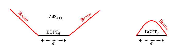
  Figure 3: BCFT with two boundaries. In the $\epsilon\to 0$ limit, the left setup leads to the duality between AdS_d+1 gravity and CFT_d-1, so-called the wedge holography. On the other hand, the right setup vanishes in this limit.

• Wedge Holography

  Recently, a new holographic duality has been proposed in [13], called wedge holography or codimension-two holography (see also [14, 93]). This is a duality between AdS_d+1 gravity and CFT_d-1. The basic idea comes from the AdS/BCFT correspondence. Let us consider a BCFT_d with two boundaries whose charges are different from each other (see the left of Figure 3). If we take the limit as the distance between two boundaries (i.e., the parameter $\epsilon$ in Figure 3) approaches zero, we can obtain a CFT_d-1, which is dual to the AdS_d+1 gravity. Since this new holography is in an early phase of investigation, many parts remain unexplained yet. For example, it is very interesting but still unclear what difference can be found in the Virasoro spectrum for the AdS₂/CFT₁ and AdS₃/CFT₁ correspondences. Our fusion matrix bootstrap in BCFTs could be useful in such a situation where we have little knowledge about the spectrum. We might be able to obtain characteristic properties of the CFT dual to the wedge, which can be compared to the AdS₃ side calculations. This type of challenge would provide new support on the wedge holography.

• Impossible brane configuration

  A brane configuration where a brane overlaps itself should be prohibited. We can translate this constraint into the CFT language by the AdS/BCFT correspondence. With this idea, some constraints have been given (for example, [94, 95], which investigate properties of the braneworld by the AdS/BCFT). It would be interesting to reproduce these types of constrains from the conformal bootstrap, because the conformal bootstrap is particularly useful to exclude impossible spectra. We would like to comment that the value $\frac{c}{32}$ discovered in [95] sometimes appear in the light-cone conformal bootstrap [96, 41, 42, 60] and the light-cone modular bootstrap [63]. Now that we have formulated the light-cone bootstrap in BCFTs, it would be interesting to investigate the relation between them.

• Some assumptions from braneworld

  In order for gravity to be localized on the brane, we need a large brane tension. Moreover, the more we decrease the brane tension, the larger the mass the graviton gets. Therefore, we have to consider the brane with the large tension if we would like to use the braneworld holography [17]. We also have some constraints from the existence of the bulk causality [97, 84]. This type of assumption appears as some constraints on the BCFT data on the BCFT side (for example, see [98, 84]). It would be interesting to make use of these assumptions to solve the bootstrap equation. In particular, it would be interesting to study whether such a theory can exist in a consistent way with the bootstrap equation.

  We can also consider a similar approach in the AdS/BCFT setup. It is naturally expected that not all boundary states can be dual to classical gravity with an EOW, only some do. Thus, we have a question, which boundary condition can have a good classical gravity description. To answer this question, it is natural to use the bootstrap equation with few known constraints from the consistency between BCFT calculations and gravity calculations (e.g., [99]). It would be interesting to further explore this direction.

• Generalization to BCFTs with other symmetries

  It would be interesting to consider a generalization of our results into a BCFT with a rich structure. For example, recently, the asymptotic behavior of the density of states transforming under a given irreducible representation of a global symmetry has been studied in [100, 101, 102, 103]. From its generalization into BCFTs, we may be able to give statements about black holes with finite group hair in the doubly holographic scenario.

Appendix A Explicit Form of Fusion Matrix

In the following, we introduce the notation usually found in Liouville CFTs.

$$c=1+6Q^{2},\ \ \ \ \ Q=b+\frac{1}{b},\ \ \ \ \ h_{i}={\alpha}_{i}(Q-{\alpha}_{i}).$$ (A.1)

Note that we can relate the parameter $\eta_{i}$ appearing in [60] to ${\alpha}_{i}$ as ${\alpha}_{i}=Q\eta_{i}$.

The fusion matrix is defined by the invertible fusion transformations between $s$ and $t$- channel conformal blocks [104] as follows:

$$\mathcal{F}^{21}_{34}(h_{{\alpha}_{s}}|z)=\int_{\mathbb{S}}{\mathrm{d}}{\alpha}_{t}{\mathbb{F}}_{{\alpha}_{s},{\alpha}_{t}}\left[\begin{array}[]{cc}{\alpha}_{2}&{\alpha}_{1}\\ {\alpha}_{3}&{\alpha}_{4}\\ \end{array}\right]\mathcal{F}^{23}_{14}(h_{{\alpha}_{t}}|1-z),$$ (A.2)

where the contour $\mathbb{S}$ runs from $\frac{Q}{2}$ to $\frac{Q}{2}+i\infty$, and also runs anti-clockwise around ${\alpha}_{t}={\alpha}_{1}+{\alpha}_{4}+mb+nb^{-1}<\frac{Q}{2}$ and ${\alpha}_{t}={\alpha}_{2}+{\alpha}_{3}+mb+nb^{-1}<\frac{Q}{2}$ for $m,n\in\mathbb{Z}_{\geq 0}$. The kernel ${\mathbb{F}}_{{\alpha}_{s},{\alpha}_{t}}$ is called the crossing matrix or fusion matrix. The explicit form of the fusion matrix is given in [105, 104]as follows:

$${\mathbb{F}}_{{\alpha}_{s},{\alpha}_{t}}\left[\begin{array}[]{cc}{\alpha}_{2}&{\alpha}_{1}\\ {\alpha}_{3}&{\alpha}_{4}\\ \end{array}\right]=\frac{N({\alpha}_{4},{\alpha}_{3},{\alpha}_{s})N({\alpha}_{s},{\alpha}_{2},{\alpha}_{1})}{N({\alpha}_{4},{\alpha}_{t},{\alpha}_{1})N({\alpha}_{t},{\alpha}_{3},{\alpha}_{2})}\left\{\begin{array}[]{cc|c}{\alpha}_{1}&{\alpha}_{2}&{\alpha}_{s}\\ {\alpha}_{3}&{\alpha}_{4}&{\alpha}_{t}\\ \end{array}\right\}_{b},$$ (A.3)

where the function $N({\alpha}_{3},{\alpha}_{2},{\alpha}_{1})$ is

$$N({\alpha}_{3},{\alpha}_{2},{\alpha}_{1})=\frac{{\Gamma}_{b}(2{\alpha}_{1}){\Gamma}_{b}(2{\alpha}_{2}){\Gamma}_{b}(2Q-2{\alpha}_{3})}{{\Gamma}_{b}(2Q-{\alpha}_{1}-{\alpha}_{2}-{\alpha}_{3}){\Gamma}_{b}(Q-{\alpha}_{1}-{\alpha}_{2}+{\alpha}_{3}){\Gamma}_{b}({\alpha}_{1}+{\alpha}_{3}-{\alpha}_{2}){\Gamma}_{b}({\alpha}_{2}+{\alpha}_{3}-{\alpha}_{1})},$$ (A.4)

and $\left\{\begin{array}[]{cc|c}{\alpha}_{1}&{\alpha}_{2}&{\alpha}_{s}\\ {\alpha}_{3}&{\alpha}_{4}&{\alpha}_{t}\\ \end{array}\right\}_{b}$ is the Racah–Wigner coefficient for the quantum group $U_{q}(sl(2,\mathbb{R}))$, which is given by

$$\left\{\begin{array}[]{cc|c}{\alpha}_{1}&{\alpha}_{2}&{\alpha}_{s}\\ {\alpha}_{3}&\bar{{\alpha}_{4}}&{\alpha}_{t}\\ \end{array}\right\}_{b}$$ (A.5)

$$=\frac{S_{b}({\alpha}_{1}+{\alpha}_{4}+{\alpha}_{t}-Q)S_{b}({\alpha}_{2}+{\alpha}_{3}+{\alpha}_{t}-Q)S_{b}({\alpha}_{3}-{\alpha}_{2}-{\alpha}_{t}+Q)S_{b}({\alpha}_{2}-{\alpha}_{3}-{\alpha}_{t}+Q)}{S_{b}({\alpha}_{1}+{\alpha}_{2}-{\alpha}_{s})S_{b}({\alpha}_{3}+{\alpha}_{s}-{\alpha}_{4})S_{b}({\alpha}_{3}+{\alpha}_{4}-{\alpha}_{s})}$$

$$\times\left|S_{b}(2{\alpha}_{t})\right|^{2}\int^{2Q+i\infty}_{2Q-i\infty}{\mathrm{d}}u\frac{S_{b}(u-{\alpha}_{12s})S_{b}(u-{\alpha}_{s34})S_{b}(u-{\alpha}_{23t})S_{b}(u-{\alpha}_{1t4})}{S_{b}(u-{\alpha}_{1234}+Q)S_{b}(u-{\alpha}_{st13}+Q)S_{b}(u-{\alpha}_{st24}+Q)S_{b}(u+Q)},$$

where we have used the notations $\bar{{\alpha}}=Q-{\alpha}$, ${\alpha}_{ijk}={\alpha}_{i}+{\alpha}_{j}+{\alpha}_{k}$ and ${\alpha}_{ijkl}={\alpha}_{i}+{\alpha}_{j}+{\alpha}_{k}+{\alpha}_{l}$. The functions ${\Gamma}_{b}(x)$ and $S_{b}(x)$ are defined as

$${\Gamma}_{b}(x)=\frac{{\Gamma}_{2}(x|b,b^{-1})}{{\Gamma}_{2}\left(\frac{Q}{2}|b,b^{-1}\right)},\ \ \ \ \ S_{b}(x)=\frac{{\Gamma}_{b}(x)}{{\Gamma}_{b}(Q-x)},$$ (A.6)

${\Gamma}_{2}(x|{\omega}_{1},{\omega}_{2})$ is the double gamma function,

$$\log{\Gamma}_{2}(x|{\omega}_{1},{\omega}_{2})=\left(\frac{\partial}{\partial t}\sum^{\infty}_{n_{1},n_{2}=0}\left(x+n_{1}{\omega}_{1}+n_{2}{\omega}_{2}\right)^{-t}\right)_{t=0}.$$ (A.7)

Note that the function ${\Gamma}_{b}(x)$ is introduced such that ${\Gamma}_{b}(x)={\Gamma}_{b^{-1}}(x)$ and satisfies the following relationship:

$${\Gamma}_{b}(x+b)=\frac{\sqrt{2\pi}b^{bx-\frac{1}{2}}}{{\Gamma}(bx)}{\Gamma}_{b}(x).$$ (A.8)

By substituting the explicit form of the Racah–Wigner coefficients (A.5) into (A.3), we can simplify the expression for the fusion matrix into

$${\mathbb{F}}_{{\alpha}_{s},{\alpha}_{t}}\left[\begin{array}[]{cc}{\alpha}_{2}&{\alpha}_{1}\\ {\alpha}_{3}&{\alpha}_{4}\\ \end{array}\right]$$ (A.9)

$$=\frac{{\Gamma}_{b}(Q+{\alpha}_{2}-{\alpha}_{3}-{\alpha}_{t}){\Gamma}_{b}(Q-{\alpha}_{2}+{\alpha}_{3}-{\alpha}_{t}){\Gamma}_{b}(2Q-{\alpha}_{1}-{\alpha}_{4}-{\alpha}_{t}){\Gamma}_{b}({\alpha}_{1}+{\alpha}_{4}-{\alpha}_{t})}{{\Gamma}_{b}(2Q-{\alpha}_{1}-{\alpha}_{2}-{\alpha}_{s}){\Gamma}_{b}({\alpha}_{1}+{\alpha}_{2}-{\alpha}_{s}){\Gamma}_{b}(Q+{\alpha}_{3}-{\alpha}_{4}-{\alpha}_{s}){\Gamma}_{b}(Q-{\alpha}_{3}+{\alpha}_{4}-{\alpha}_{s})}$$

$$\times\frac{{\Gamma}_{b}(Q-{\alpha}_{2}-{\alpha}_{3}+{\alpha}_{t}){\Gamma}(-Q+{\alpha}_{2}+{\alpha}_{3}+{\alpha}_{t}){\Gamma}_{b}({\alpha}_{1}-{\alpha}_{4}+{\alpha}_{t}){\Gamma}_{b}(-{\alpha}_{1}+{\alpha}_{4}+{\alpha}_{t})}{{\Gamma}_{b}({\alpha}_{1}-{\alpha}_{2}+{\alpha}_{s}){\Gamma}_{b}(-{\alpha}_{1}+{\alpha}_{2}+{\alpha}_{s}){\Gamma}_{b}(Q-{\alpha}_{3}-{\alpha}_{4}+{\alpha}_{s}){\Gamma}_{b}(-Q+{\alpha}_{3}+{\alpha}_{4}+{\alpha}_{s})}$$

$$\times\left|S_{b}(2{\alpha}_{t})\right|^{2}\frac{{\Gamma}_{b}(2Q-2{\alpha}_{s}){\Gamma}_{b}(2{\alpha}_{s})}{{\Gamma}_{b}(2Q-2{\alpha}_{t}){\Gamma}_{b}(2{\alpha}_{t})}$$

$$\times\int^{2Q+i\infty}_{2Q-i\infty}{\mathrm{d}}u\frac{S_{b}(u-{\alpha}_{12s})S_{b}(u-{\alpha}_{s34})S_{b}(u-{\alpha}_{23t})S_{b}(u-{\alpha}_{1t4})}{S_{b}(u-{\alpha}_{1234}+Q)S_{b}(u-{\alpha}_{st13}+Q)S_{b}(u-{\alpha}_{st24}+Q)S_{b}(u+Q)}.$$

References

- [1] G. Penington, Entanglement wedge reconstruction and the information paradox, JHEP 09 (2020) 002 [1905.08255].
- [2] A. Almheiri, N. Engelhardt, D. Marolf and H. Maxfield, The entropy of bulk quantum fields and the entanglement wedge of an evaporating black hole, JHEP 12 (2019) 063 [1905.08762].
- [3] A. Almheiri, R. Mahajan, J. Maldacena and Y. Zhao, The page curve of hawking radiation from semiclassical geometry, JHEP 03 (2020) 149 [1908.10996].
- [4] J.M. Maldacena, The large n limit of superconformal field theories and supergravity, Adv. Theor. Math. Phys. 2 (1998) 231 [hep-th/9711200].
- [5] T. Takayanagi, Holographic dual of bcft, Phys. Rev. Lett. 107 (2011) 101602 [1105.5165].
- [6] M. Fujita, T. Takayanagi and E. Tonni, Aspects of ads/bcft, JHEP 11 (2011) 043 [1108.5152].
- [7] D.S. Ageev, Shaping contours of entanglement islands in BCFT, 2107.09083.
- [8] I. Akal, Y. Kusuki, N. Shiba, T. Takayanagi and Z. Wei, Holographic moving mirrors, Class. Quant. Grav. 38 (2021) 224001 [2106.11179].
- [9] J. Chu, F. Deng and Y. Zhou, Page curve from defect extremal surface and island in higher dimensions, JHEP 10 (2021) 149 [2105.09106].
- [10] R. Bousso and E. Wildenhain, Gravity/ensemble duality, Phys. Rev. D 102 (2020) 066005 [2006.16289].
- [11] J. Sully, M.V. Raamsdonk and D. Wakeham, BCFT entanglement entropy at large central charge and the black hole interior, JHEP 03 (2021) 167 [2004.13088].
- [12] I. Akal, Y. Kusuki, N. Shiba, T. Takayanagi and Z. Wei, Entanglement entropy in a holographic moving mirror and the page curve, Phys. Rev. Lett. 126 (2021) 061604 [2011.12005].
- [13] I. Akal, Y. Kusuki, T. Takayanagi and Z. Wei, Codimension two holography for wedges, Phys. Rev. D 102 (2020) 126007 [2007.06800].
- [14] R.-X. Miao, An exact construction of codimension two holography, JHEP 01 (2021) 150 [2009.06263].
- [15] H. Geng, A. Karch, C. Perez-Pardavila, S. Raju, L. Randall, M. Riojas et al., Information transfer with a gravitating bath, SciPost Phys. 10 (2021) 103 [2012.04671].
- [16] H. Geng, A. Karch, C. Perez-Pardavila, S. Raju, L. Randall, M. Riojas et al., Entanglement phase structure of a holographic bcft in a black hole background, 2112.09132.
- [17] A. Karch and L. Randall, Locally localized gravity, JHEP 05 (2001) 008 [hep-th/0011156].
- [18] L. Randall and R. Sundrum, A large mass hierarchy from a small extra dimension, Phys. Rev. Lett. 83 (1999) 3370 [hep-ph/9905221].
- [19] L. Randall and R. Sundrum, An alternative to compactification, Phys. Rev. Lett. 83 (1999) 4690 [hep-th/9906064].
- [20] J. Teschner, Remarks on liouville theory with boundary, PoS tmr2000 (2000) 041 [hep-th/0009138].
- [21] B. Ponsot and J. Teschner, Boundary liouville field theory: Boundary three point function, Nucl. Phys. B 622 (2002) 309 [hep-th/0110244].
- [22] V. Fateev, A.B. Zamolodchikov and A.B. Zamolodchikov, Boundary liouville field theory. 1. boundary state and boundary two point function, hep-th/0001012.
- [23] S. Collier, D. Mazac and Y. Wang, Bootstrapping boundaries and branes, 2112.00750.
- [24] J.L. Cardy, Boundary conformal field theory, hep-th/0411189.
- [25] J.L. Cardy, Operator content of two-dimensional conformally invariant theories, Nucl. Phys. B 270 (1986) 186.
- [26] A. Strominger and C. Vafa, Microscopic origin of the bekenstein-hawking entropy, Phys. Lett. B 379 (1996) 99 [hep-th/9601029].
- [27] R. Rattazzi, V.S. Rychkov, E. Tonni and A. Vichi, Bounding scalar operator dimensions in 4d cft, JHEP 12 (2008) 031 [0807.0004].
- [28] V.S. Rychkov and A. Vichi, Universal constraints on conformal operator dimensions, Phys. Rev. D 80 (2009) 045006 [0905.2211].
- [29] F. Kos, D. Poland and D. Simmons-Duffin, Bootstrapping mixed correlators in the 3d ising model, JHEP 11 (2014) 109 [1406.4858].
- [30] D. Simmons-Duffin, A semidefinite program solver for the conformal bootstrap, JHEP 06 (2015) 174 [1502.02033].
- [31] S. Collier, Y.-H. Lin and X. Yin, Modular bootstrap revisited, JHEP 09 (2018) 061 [1608.06241].
- [32] S. Hellerman, A universal inequality for cft and quantum gravity, JHEP 08 (2011) 130 [0902.2790].
- [33] D. Friedan and C.A. Keller, Constraints on 2d cft partition functions, JHEP 10 (2013) 180 [1307.6562].
- [34] T. Hartman, D. Mazáč and L. Rastelli, Sphere Packing and Quantum Gravity, JHEP 12 (2019) 048 [1905.01319].
- [35] N. Afkhami-Jeddi, T. Hartman and A. Tajdini, Fast conformal bootstrap and constraints on 3d gravity, JHEP 05 (2019) 087 [1903.06272].
- [36] M. Besken, Virasoro conformal bootstrap with , 2106.08999.
- [37] S. Collier, P. Kravchuk, Y.-H. Lin and X. Yin, Bootstrapping the spectral function: On the uniqueness of liouville and the universality of btz, JHEP 09 (2018) 150 [1702.00423].
- [38] B. Mukhametzhanov and A. Zhiboedov, Modular invariance, tauberian theorems and microcanonical entropy, JHEP 10 (2019) 261 [1904.06359].
- [39] S. Pal and Z. Sun, Tauberian-cardy formula with spin, JHEP 01 (2020) 135 [1910.07727].
- [40] D. Das, S. Datta and S. Pal, Universal asymptotics of three-point coefficients from elliptic representation of virasoro blocks, Phys. Rev. D 98 (2018) 101901 [1712.01842].
- [41] Y. Kusuki, Large c virasoro blocks from monodromy method beyond known limits, JHEP 08 (2018) 161 [1806.04352].
- [42] Y. Kusuki, New properties of large- conformal blocks from recursion relation, JHEP 07 (2018) 010 [1804.06171].
- [43] D. Das, Y. Kusuki and S. Pal, Universality in asymptotic bounds and its saturation in d cft, JHEP 04 (2021) 288 [2011.02482].
- [44] I. Tsiares, Universal dynamics in non-orientable cft2, 2011.09250.
- [45] P. Kraus and A. Maloney, A cardy formula for three-point coefficients or how the black hole got its spots, JHEP 05 (2017) 160 [1608.03284].
- [46] Y. Hikida, Y. Kusuki and T. Takayanagi, Eigenstate thermalization hypothesis and modular invariance of two-dimensional conformal field theories, Phys. Rev. D 98 (2018) 026003 [1804.09658].
- [47] A. Romero-Bermúdez, P. Sabella-Garnier and K. Schalm, A cardy formula for off-diagonal three-point coefficients; or, how the geometry behind the horizon gets disentangled, JHEP 09 (2018) 005 [1804.08899].
- [48] E.M. Brehm, D. Das and S. Datta, Probing thermality beyond the diagonal, Phys. Rev. D 98 (2018) 126015 [1804.07924].
- [49] J. Cardy, A. Maloney and H. Maxfield, A new handle on three-point coefficients: Ope asymptotics from genus two modular invariance, JHEP 10 (2017) 136 [1705.05855].
- [50] A.L. Fitzpatrick, J. Kaplan, D. Poland and D. Simmons-Duffin, The analytic bootstrap and ads superhorizon locality, JHEP 12 (2013) 004 [1212.3616].
- [51] Z. Komargodski and A. Zhiboedov, Convexity and liberation at large spin, JHEP 11 (2013) 140 [1212.4103].
- [52] L.F. Alday, A. Bissi and T. Lukowski, Large spin systematics in cft, JHEP 11 (2015) 101 [1502.07707].
- [53] A. Kaviraj, K. Sen and A. Sinha, Analytic bootstrap at large spin, JHEP 11 (2015) 083 [1502.01437].
- [54] A. Kaviraj, K. Sen and A. Sinha, Universal anomalous dimensions at large spin and large twist, JHEP 07 (2015) 026 [1504.00772].
- [55] L.F. Alday and A. Zhiboedov, An algebraic approach to the analytic bootstrap, JHEP 04 (2017) 157 [1510.08091].
- [56] D. Simmons-Duffin, The lightcone bootstrap and the spectrum of the 3d ising cft, JHEP 03 (2017) 086 [1612.08471].
- [57] L.F. Alday, Large spin perturbation theory for conformal field theories, Phys. Rev. Lett. 119 (2017) 111601 [1611.01500].
- [58] C. Sleight and M. Taronna, Anomalous dimensions from crossing kernels, JHEP 11 (2018) 089 [1807.05941].
- [59] A.L. Fitzpatrick, J. Kaplan and M.T. Walters, Universality of long-distance ads physics from the cft bootstrap, JHEP 08 (2014) 145 [1403.6829].
- [60] Y. Kusuki, Light cone bootstrap in general 2d cfts and entanglement from light cone singularity, JHEP 01 (2019) 025 [1810.01335].
- [61] Y. Kusuki and M. Miyaji, Entanglement entropy, otoc and bootstrap in 2d cfts from regge and light cone limits of multi-point conformal block, JHEP 08 (2019) 063 [1905.02191].
- [62] H. Maxfield, Quantum corrections to the btz black hole extremality bound from the conformal bootstrap, JHEP 12 (2019) 003 [1906.04416].
- [63] N. Benjamin, H. Ooguri, S.-H. Shao and Y. Wang, Light-cone modular bootstrap and pure gravity, Phys. Rev. D 100 (2019) 066029 [1906.04184].
- [64] N. Benjamin, S. Collier and A. Maloney, Pure gravity and conical defects, JHEP 09 (2020) 034 [2004.14428].
- [65] E.M. Brehm and D. Das, Aspects of the s transformation bootstrap, J. Stat. Mech. 2005 (2020) 053103 [1911.02309].
- [66] S. Collier, A. Maloney, H. Maxfield and I. Tsiares, Universal dynamics of heavy operators in cft2, JHEP 07 (2020) 074 [1912.00222].
- [67] T. Anous, A. Belin, J. de Boer and D. Liska, Ope statistics from higher-point crossing, 2112.09143.
- [68] D.C. Lewellen, Sewing constraints for conformal field theories on surfaces with boundaries, Nucl. Phys. B 372 (1992) 654.
- [69] D. Mazac, Analytic bounds and emergence of AdS2 physics from the conformal bootstrap, JHEP 04 (2017) 146 [1611.10060].
- [70] D. Mazac and M.F. Paulos, The analytic functional bootstrap. Part I: 1D CFTs and 2D S-matrices, JHEP 02 (2019) 162 [1803.10233].
- [71] A.L. Fitzpatrick, J. Kaplan and M.T. Walters, Virasoro conformal blocks and thermality from classical background fields, JHEP 11 (2015) 200 [1501.05315].
- [72] A.L. Fitzpatrick, J. Kaplan, D. Li and J. Wang, On information loss in ads3/cft2, JHEP 05 (2016) 109 [1603.08925].
- [73] S. Collier, Y. Gobeil, H. Maxfield and E. Perlmutter, Quantum regge trajectories and the virasoro analytic bootstrap, JHEP 05 (2019) 212 [1811.05710].
- [74] S. He, Conformal bootstrap to rényi entropy in 2d liouville and super-liouville cfts, Phys. Rev. D 99 (2019) 026005 [1711.00624].
- [75] J.L. Cardy and D.C. Lewellen, Bulk and boundary operators in conformal field theory, Phys. Lett. B 259 (1991) 274.
- [76] H. Sonoda, Sewing conformal field theories, Nucl. Phys. B 311 (1988) 401.
- [77] G.W. Moore and N. Seiberg, Classical and quantum conformal field theory, Commun. Math. Phys. 123 (1989) 177.
- [78] G.W. Moore and N. Seiberg, Naturality in conformal field theory, Nucl. Phys. B 313 (1989) 16.
- [79] G.W. Moore and N. Seiberg, Polynomial equations for rational conformal field theories, Phys. Lett. B 212 (1988) 451.
- [80] J. Sully, M.V. Raamsdonk and D. Wakeham, Bcft entanglement entropy at large central charge and the black hole interior, JHEP 03 (2021) 167 [2004.13088].
- [81] J. Teschner, From liouville theory to the quantum geometry of riemann surfaces, in 14th International Congress on Mathematical Physics, 8, 2003 [hep-th/0308031].
- [82] M. Cadoni, P. Carta and S. Mignemi, The cardy-verlinde formula for 2d gravity, Nucl. Phys. B 632 (2002) 383 [hep-th/0202180].
- [83] T. Hartman, C.A. Keller and B. Stoica, Universal spectrum of 2d conformal field theory in the large c limit, JHEP 09 (2014) 118 [1405.5137].
- [84] W. Reeves, M. Rozali, P. Simidzija, J. Sully, C. Waddell and D. Wakeham, Looking for (and not finding) a bulk brane, 2108.10345.
- [85] M. Srednicki, The approach to thermal equilibrium in quantized chaotic systems, J. Phys. A 32 (1999) 1163 (1998) [cond-mat/9809360].
- [86] L. D’Alessio, Y. Kafri, A. Polkovnikov and M. Rigol, From quantum chaos and eigenstate thermalization to statistical mechanics and thermodynamics, Adv. Phys. 65 (2016) 239 [1509.06411].
- [87] R. Mondaini and M. Rigol, Eigenstate thermalization in the two-dimensional transverse field ising model: Ii. off-diagonal matrix elements of observables, Phys. Rev. E 96, 012157 (2017) (2017) [1705.08058].
- [88] B. Mukhametzhanov and S. Pal, Beurling-selberg extremization and modular bootstrap at high energies, SciPost Phys. 8 (2020) 088 [2003.14316].
- [89] J. Qiao and S. Rychkov, A tauberian theorem for the conformal bootstrap, 1709.00008.
- [90] A. Maloney and E. Witten, Quantum gravity partition functions in three dimensions, JHEP 02 (2010) 029 [0712.0155].
- [91] Y.-k. Suzuki, One-loop correction to the ads/bcft partition function in the three dimensional pure gravity, 2106.00206.
- [92] A. Belin, S. Biswas and J. Sully, The spectrum of boundary states in symmetric orbifolds, 2110.05491.
- [93] R.-X. Miao, Codimension-n holography for cones, Phys. Rev. D 104 (2021) 086031 [2101.10031].
- [94] S. Cooper, M. Rozali, B. Swingle, M. Van Raamsdonk, C. Waddell and D. Wakeham, Black hole microstate cosmology, JHEP 07 (2019) 065 [1810.10601].
- [95] H. Geng, S. Lüst, R.K. Mishra and D. Wakeham, Holographic BCFTs and Communicating Black Holes, jhep 08 (2021) 003 [2104.07039].
- [96] Y. Kusuki and T. Takayanagi, Renyi entropy for local quenches in 2d cft from numerical conformal blocks, JHEP 01 (2018) 115 [1711.09913].
- [97] H. Omiya and Z. Wei, Causal structures and nonlocality in double holography, 2107.01219.
- [98] O. Aharony, O. DeWolfe, D.Z. Freedman and A. Karch, Defect conformal field theory and locally localized gravity, JHEP 07 (2003) 030 [hep-th/0303249].
- [99] J. Kastikainen and S. Shashi, Structure of holographic bcft correlators from geodesics, 2109.00079.
- [100] D. Harlow and H. Ooguri, A universal formula for the density of states in theories with finite-group symmetry, 2109.03838.
- [101] J.M. Magan, Proof of the universal density of charged states in qft, JHEP 12 (2021) 100 [2111.02418].
- [102] W. Cao, T. Melia and S. Pal, Universal fine grained asymptotics of weakly coupled quantum field theory, 2111.04725.
- [103] S. Pal and Z. Sun, High energy modular bootstrap, global symmetries and defects, JHEP 08 (2020) 064 [2004.12557].
- [104] J. Teschner, Liouville theory revisited, Class. Quant. Grav. 18 (2001) R153 [hep-th/0104158].
- [105] B. Ponsot and J. Teschner, Liouville bootstrap via harmonic analysis on a noncompact quantum group, hep-th/9911110.
- [106] J. Teschner and G. Vartanov, 6j symbols for the modular double, quantum hyperbolic geometry, and supersymmetric gauge theories, Lett. Math. Phys. 104 (2014) 527 [1202.4698].