Infinite energy cavitating solutions: a variational approach

Abstract

We study the phenomenon of cavitation for the displacement boundary-value problem of radial, isotropic compressible elasticity for a class of stored energy functions of the form $W(F)+h(\det F)$, where $W$ grows like $\left\|F\right\|^{n}$, and $n$ is the space dimension. In this case it follows (from a result of Vodop’yanov, Gol’dshtein and Reshetnyak) that discontinuous deformations must have infinite energy. After characterizing the rate at which this energy blows up, we introduce a modified energy functional which differs from the original by a null lagrangian, and for which cavitating energy minimizers with finite energy exist. In particular, the Euler–Lagrange equations for the modified energy functional are identical to those for the original problem except for the boundary condition at the inner cavity. This new boundary condition states that a certain modified radial Cauchy stress function has to vanish at the inner cavity. This condition corresponds to the radial Cauchy stress for the original functional diverging to $-\infty$ at the cavity surface. Many previously known variational results for finite energy cavitating solutions now follow for the modified functional, such as the existence of radial energy minimizers, satisfaction of the Euler-Lagrange equations for such minimizers, and the existence of a critical boundary displacement for cavitation. We also discuss a numerical scheme for computing these singular cavitating solutions using regular solutions for punctured balls. We show the convergence of this numerical scheme and give some numerical examples including one for the incompressible limit case. Our approach is motivated in part by the use of the “renormalized energy” for Ginzberg-Landau vortices.

Key words: nonlinear elasticity, cavitation, infinite energy solutions.

AMS subject classifications: 74B20, 93B40, 65K10

1 Introduction

Cavitation (i.e., the formation of holes) is a commonly observed phenomenon in the fracture of polymers and metals (see [5]). In his seminal paper [1], Ball formulated a variational problem, in the setting of nonlinear elasticity, for which the energy minimising radial deformations of (an initially solid) ball formed a cavity at the centre of the deformed ball when the imposed boundary loads or displacements were sufficiently large. Following this paper there have been numerous studies of aspects of the problem of radial cavitation: some on analytical properties (see, e.g., [23], [18], [13]) and others relating to specific stored energies (a helpful overview is contained in [11]). Subsequent studies, e.g., of [14], [19], [12], [8] have addressed general analytic questions of existence of cavitating energy minimisers in the non–symmetric case. In all of these works, the Dirichlet part of the stored energy function grows like $\left\|\nabla\mathbf{u}\right\|^{p}$ with $n-1<p<n$, where $\mathbf{u}$ is a deformation and $n$ is the space dimension. The case $p=n-1$ for non cavitating deformations and for a three dimensional compressible neo–Hookean material ([17]), has been studied in [10] for axisymmetric bodies.

In this paper we study radial solutions of the equations of elasticity for a spherically symmetric, isotropic, hyperelastic, compressible body, for the critical exponent $p=n$. It follows in this case that cavitating solutions for the corresponding Euler–Lagrange equations have infinite energy. Using a variational approach, we show that for a general class of stored energy functions, the radial equilibrium equations do have cavitating solutions with infinite Cauchy stress at the origin and satisfying the outer displacement boundary condition. Moreover these solutions are characterized as finite energy minimizers of a modified energy functional (cf. (34)) with the same equilibrium equations as the original functional. Our approach has connections with work of Henao and Serfaty [9] and Cañulef-Aguilar and Henao [3] for incompressible materials and with the use of the ”renormalised” energy in the Ginzberg-Landau vortices problem [2].

The case $n=2$ of this problem, which corresponds to a two dimensional compressible neo–Hookean material, was studied by Ball [1, pp. 606-607] where he proved, for a particular stored energy function having logarithmic growth for small determinants, the existence of cavitating solutions of the equilibrium equations having infinite Cauchy stress at the origin. His approach is based on an application of Schauder’s fixed point theorem, and although he did not solve the full boundary value problem (there was no attempt to match the outer boundary condition), the cavity size appears as a parameter in his argument which in principle could be adjusted to match the outer boundary condition. The class of stored energy functions studied in this paper (cf. (20)) includes compressible neo-Hookean stored energies widely used in applications. The results of this paper, in the case $n=2$, thus allow for a variational treatment of cavitation of a disc in two dimensions, which has not been previously possible for such neo–Hookean stored energy functions. The approach should also extend to treat axisymmetric cavitation of a cylinder in three dimensions (the work in [10] on axisymmetric deformations may be relevant here).

Consider a body which in its reference configuration occupies the region

$$\mathcal{B}=\{\mathbf{x}\in\mathbb{R}^{n}~{}:~{}\left\|\mathbf{x}\right\|<1\},$$ (1)

where $n=2,3$ and $\left\|\cdot\right\|$ denotes the Euclidean norm. Let $\mathbf{u}:\mathcal{B}\rightarrow\mathbb{R}^{n}$ denote a deformation of the body and let its deformation gradient be

$$\nabla\mathbf{u}(\mathbf{x})=\frac{\mathrm{d}\mathbf{u}}{\mathrm{d}\mathbf{x}}(\mathbf{x}).$$ (2)

For smooth deformations, the requirement that $\mathbf{u}(\mathbf{x})$ is locally invertible and preserves orientation takes the form

$$\det\nabla\mathbf{u}(\mathbf{x})>0,\quad\mathbf{x}\in\mathcal{B}.$$ (3)

Let $W:M_{+}^{n\times n}\rightarrow\mathbb{R}$ be the stored energy function of the material of the body where $M_{+}^{n\times n}=\{\mathbf{F}\in M^{n\times n}~{}:~{}\det\mathbf{F}>0\}$ and $M^{n\times n}$ denotes the space of real $n\times n$ matrices. We assume that the stored energy function $W$ satisfies $W\rightarrow\infty$ as either $\det\mathbf{F}\rightarrow 0^{+}$ or $\left\|\mathbf{F}\right\|\rightarrow\infty$. The total energy stored in the body due to the deformation $\mathbf{u}$ is given by

$$E(\mathbf{u})=\int_{\mathcal{B}}W(\nabla\mathbf{u}(\mathbf{x}))\,\mathrm{d}\mathbf{x}.$$ (4)

We consider the problem of determining a configuration of the body that satisfies (3) almost everywhere and minimizes (4) among all functions satisfying the boundary condition:

$$\mathbf{u}(\mathbf{x})=\lambda\mathbf{x},\quad\mathbf{x}\in\partial\mathcal{B},$$ (5)

where $\lambda>0$ is given. Formally, a sufficiently smooth minimizer satisfies the equilibrium equations

$$\mathrm{div\,}\left[\frac{\mathrm{d}W}{\mathrm{d}\mathbf{F}}(\nabla\mathbf{u}(\mathbf{x}))\right]=\mathbf{0}.$$ (6)

Note that if the stored energy $W$ satisfies a growth condition of the form

$$c_{1}\left\|\mathbf{F}\right\|^{n}+c_{2}\leq W(\mathbf{F}),\quad\forall\,\mathbf{F}\mbox{ with }\det\mathbf{F}>0,$$ (7)

then (cf. [25]) any discontinuous deformation ${\mathbf{u}}$ of $\mathcal{B}$ with $\det\nabla{\mathbf{u}}>0$ a.e., must have infinite energy.

For later reference we mention that if $\mathbf{u}$ is a smooth solution of (6), then (see [7])

$$\mathrm{div\,}\left[W(\nabla\mathbf{u})\mathbf{x}+\left[\frac{\partial W}{\partial\mathbf{F}}(\nabla\mathbf{u})\right]^{T}\!\!(\mathbf{u}-(\nabla\mathbf{u})\mathbf{x})\right]=nW(\nabla\mathbf{u}).$$ (8)

If $\mathbf{u}$ is smooth except at the origin where it opens up a cavity, and $\mathcal{B}_{\varepsilon}$ is a ball of radius $\varepsilon>0$ around the origin, then integrating this equation over the punctured ball $\mathcal{B}\setminus\mathcal{B}_{\varepsilon}$, we get that

$$n\int_{\mathcal{B}\setminus\mathcal{B}_{\varepsilon}}W(\nabla\mathbf{u}(\mathbf{x}))\,\mathrm{d}\mathbf{x} = \int_{\partial\mathcal{B}}\left[W(\nabla\mathbf{u})\mathbf{x}+\left[\frac{\partial W}{\partial\mathbf{F}}(\nabla\mathbf{u})\right]^{T}\!\!(\mathbf{u}-(\nabla\mathbf{u})\mathbf{x})\right]\cdot{\mathbf{N}}\,\mathrm{d}s(\mathbf{x})$$ (9)

$$-\int_{\partial\mathcal{B}_{\varepsilon}}\left[W(\nabla\mathbf{u})\mathbf{x}+\left[\frac{\partial W}{\partial\mathbf{F}}(\nabla\mathbf{u})\right]^{T}\!\!(\mathbf{u}-(\nabla\mathbf{u})\mathbf{x})\right]\cdot{\mathbf{N}}\,\mathrm{d}s(\mathbf{x}),$$

where $\mathbf{N}$ is the outer normal to each boundary. Thus the blow up in the energy as $\varepsilon$ becomes small, comes from the integral over the boundary $\partial\mathcal{B}_{\varepsilon}$. Note that this integral is the sum of two terms:

$$\int_{\partial\mathcal{B}_{\varepsilon}}\left[W(\nabla\mathbf{u})\mathbf{I}-\left[\frac{\partial W}{\partial\mathbf{F}}(\nabla\mathbf{u})\right]^{T}\!\!(\nabla\mathbf{u})\right]\mathbf{x}\cdot{\mathbf{N}}\,\mathrm{d}s(\mathbf{x}),\,\,\int_{\partial\mathcal{B}_{\varepsilon}}\left[\frac{\partial W}{\partial\mathbf{F}}(\nabla\mathbf{u})\right]^{T}\!\!\mathbf{u}\cdot{\mathbf{N}}\,\mathrm{d}s(\mathbf{x}),$$ (10)

the second one representing as $\varepsilon\rightarrow 0$, the work done in opening the singularity. The tensor in brackets in the first boundary integral above is the Eshelby energy–momentum tensor (cf. [4], [6]). It is interesting to note that if the stored energy function grows like $\left\|\nabla\mathbf{u}\right\|^{p}$, then for $p<n$ both terms in (10) tend to zero as $\varepsilon\rightarrow 0$ (cf. [20]), while both tend to infinity if $p>n$. In the case $p=n$ and in the radial case, we will show that the first term has a finite limit while the second one is unbounded as $\varepsilon\rightarrow 0$.

If the material is homogeneous and $W$ is isotropic and frame indifferent, then it follows that

$$W(\mathbf{F})=\Phi(v_{1},\ldots,v_{n}),\quad\mathbf{F}\in M_{+}^{n\times n},$$ (11)

for some function $\Phi:\mathbb{R}_{+}^{n}\rightarrow\mathbb{R}$ symmetric in its arguments, where $v_{1},\ldots,v_{n}$ are the eigenvalues of $(\mathbf{F}^{t}\mathbf{F})^{1/2}$ known as the principal stretches.

We now restrict attention to the special case in which the deformation $\mathbf{u}(\cdot)$ is radially symmetric, so that

$$\mathbf{u}(\mathbf{x})=r(R)\,\frac{\mathbf{x}}{R},\quad\mathbf{x}\in\mathcal{B},$$ (12)

for some scalar function $r(\cdot)$, where $R=\left\|\mathbf{x}\right\|$. In this case one can easily check that

$$v_{1}=r^{\prime}(R)~{}~{},~{}~{}v_{2}=\cdots=v_{n}=\frac{r(R)}{R}.$$ (13)

Thus (4) reduces to

$$E(\mathbf{u})=\omega_{n}I(r)=\omega_{n}\int_{0}^{1}R^{n-1}\Phi\left(r^{\prime}(R),\frac{r(R)}{R},\ldots,\frac{r(R)}{R}\right)\,\mathrm{d}R,$$ (14)

where $\omega_{n}=2\pi$ or $\omega_{n}=4\pi$ if $n=2\ \mathrm{or}\ 3$ respectively. (In general $\omega_{n}$ is area of the unit sphere in $\mathbb{R}^{n}$.)

In accord with (3) we have the inequalities

$$r^{\prime}(R),\,\frac{r(R)}{R}>0,\quad 0<R<1,$$ (15)

and (5) reduces to:

$$r(1)=\lambda.$$ (16)

Our problem now is to minimize the functional $I(\cdot)$ over the set

$$\mathcal{A}_{\lambda}=\left\{r\in W^{1,1}(0,1)\,:\,r(1)=\lambda,\,r^{\prime}(R)>0\mbox{ for~{}a.e.~{}}R\in(0,1),\,r(0)\geq 0\right\}.$$ (17)

Formally, the Euler–Lagrange equation for $I(\cdot)$ is given by

$$\frac{\mathrm{d}}{\mathrm{d}R}\left[R^{n-1}\Phi_{,1}(r(R))\right]=(n-1)R^{n-2}\Phi_{,2}(r(R)),\quad 0<R<1,$$ (18)

subject to (16) and $r(0)\geq 0$, where:

$$\Phi_{,i}(r(R))=\Phi_{,i}\left(r^{\prime}(R),\displaystyle\frac{r(R)}{R},\ldots,\frac{r(R)}{R}\right),\ \ \ i=1,...,n.$$ (19)

If $c=r(0)>0$, then the deformed ball contains a spherical cavity of radius $c$. In the case $n=2$, Ball [1, pp. 606-607] gives an example of a stored energy function satisfying (7) and proves existence of corresponding radial cavitating equilibrium solutions of (18) which (necessarily) have infinite energy. His approach is based on an application of Schauder’s fixed point theorem, and although he does not solve the full boundary-value problem (there was no attempt to match the outer boundary condition), the cavity size appears as a parameter in his argument which, in principle, could be adjusted to match the outer boundary condition. In this paper we give a characterization of cavitating equilibria with infinite energy as minimizers of a modified energy functional, which is related to the growth of the radial component of the Cauchy stress of an equilibrium solution near a point of cavitation.

To highlight some of the general structure of the underlying problem, we will state certain of our results for stored energy functions of the form

$$\Phi(v_{1},\ldots,v_{n})=\frac{\kappa}{n}\sum_{i=1}^{n}v_{i}^{n}+h(v_{1}v_{2}\cdots v_{n}),$$ (20)

where $\kappa>0$ and $h\,:\,(0,\infty)\rightarrow[0,\infty)$ is a $C^{1}$ function that satisfies

$$h^{\prime\prime}(d)>0, \forall\,d>0,$$ (21a)

$$\lim_{d\rightarrow 0^{+}}h(d)=\infty, \lim_{d\rightarrow\infty}\frac{h(d)}{d}=\infty,$$ (21b)

$$\lim_{d\rightarrow 0^{+}}h^{\prime}(d)=-\infty, \lim_{d\rightarrow\infty}h^{\prime}(d)=\infty.$$ (21c)

In this case, the energy functional $I(r)$ in (14) takes the form

$$I(r)=\int_{0}^{1}R^{n-1}\left[\frac{\kappa}{n}\left((r^{\prime}(R))^{n}+(n-1)\left(\frac{r(R)}{R}\right)^{n}\right)+h(\delta(R))\right]\,dR,$$ (22)

where

$$\delta(R)=r^{\prime}(R)\left(\frac{r(R)}{R}\right)^{n-1}.$$

It is clear that (discontinuous) radial deformations with $r(0)>0$ must have infinite energy as a result of the second bracketed term in the integrand. In Section 2, in the spirit of the “renormalized energy approach” for Ginzberg-Landau vortices (see, e.g., [2]), we characterize the order of the singularity in the energy and in the radial component of Cauchy stress for a cavitating solution as logarithmic in all dimensions. To motivate the form of the regularisation, we use the specialization of (8) to the radial case satisfied by smooth solutions of the radial equilibrium equation (18):

$$R^{n-1}\Phi(r(R))=\frac{d}{dR}\left[\frac{R^{n}}{n}\left(\Phi(r(R))-r^{\prime}\Phi_{,1}(r(R))\right)+\frac{r^{n}}{n}T(r(R))\right],$$ (23)

with the notation in (19) and where

$$T(r(R))=\left[\frac{R}{r(R)}\right]^{n-1}\Phi_{,1}(r(R)),$$ (24)

is the radial component of the Cauchy stress. Integrating the above identity from $R=\varepsilon$ to $R=1$ for a cavitating solution and using the form of the stored energy function (20), we show that all boundary terms have a finite limit as $\epsilon\rightarrow 0$ apart from the term

$$-\lim_{\epsilon\rightarrow 0}\frac{r(\epsilon)^{n}}{n}\,T(r(\epsilon)),$$ (25)

which corresponds to the second term in (10). Thus, the infinite energy of a radial solution of the equilibrium equation with $r(0)>0$ corresponds to a singularity in the radial Cauchy stress. Thus the term (25) can be formally interpreted as the (infinite) work required to open the cavity. (If $r(0)=0$, then this term is zero.) Thus for a cavitating solution

$$\lim_{\varepsilon\rightarrow 0}\left[\int_{\varepsilon}^{1}R^{n-1}\Phi\left(r^{\prime}(R),\frac{r(R)}{R},\ldots,\frac{r(R)}{R}\right)\,dR+\frac{r(\epsilon)^{n}}{n}\,T(r(\epsilon))\right],$$

is finite. Using the characterization of the asymptotic behaviour of the Cauchy stress given in Proposition 2.2, we introduce a modified energy functional, given by

$$\hat{I}(r) = \int_{0}^{1}R^{n-1}\Phi\left(r^{\prime}(R),\frac{r(R)}{R},\ldots,\frac{r(R)}{R}\right)\,dR$$ (26)

$$-\dfrac{\kappa(n-1)}{n}\lim_{R\rightarrow 0}r^{n}(R)\ln\left(\frac{r(R)}{R}\right),$$

where the last term accounts for the singular behaviour in (25). This functional can also be expressed as

$$\hat{I}(r) = \int_{0}^{1}R^{n-1}\left[\frac{\kappa}{n}\left(r^{\prime}\right)^{n}+h\left(\delta(R)\right)+\kappa(n-1)\delta(R)\left(\dfrac{1}{n}+\ln\left(\frac{r}{R}\right)\right)\right]\,\mathrm{d}R$$

$$~{}~{}~{}~{}~{}~{}~{}~{}~{}~{}~{}~{}~{}~{}~{}~{}~{}~{}~{}~{}~{}~{}-\frac{\kappa(n-1)}{n}\lambda^{n}\ln\lambda.$$

It is easy to now show that there are $r\in\mathcal{A}_{\lambda}$, with $r(0)>0$ for which $\hat{I}(r)$ is finite. Moreover, the Euler-Lagrange equation for this modified functional coincides with that for the original functional (22) since, by construction, they differ by a null lagrangian term (see Theorem 3.3). Moreover, for many deformations with $r(0)=0$, in particular for the homogeneous deformation $r(R)\equiv\lambda R$, the two energies coincide. However, we will show that for $\lambda$ sufficiently large, energy minimisers for the modified functional must satisfy $r(0)>0$.

Many known results for finite energy cavitating solutions (see, e.g., [1], [23], [18]) now follow by similar methods for the modified functional (26). In particular in Section 3 we show that minimizers of the modified functional exist and that they satisfy the corresponding Euler-Lagrange equations for such minimizers. Moreover, in Theorem 3.6 we show the existence of a critical boundary displacement $\lambda_{c}$ for cavitation for the modified functional, below of which the minimizers of the modified functional must be homogeneous.

In Section 4 we discuss a numerical scheme for computing the cavitating solutions of the modified functional via solutions on punctured balls. In the usual cavitation problem, the convergence of the solutions on these punctured balls to a solution on the full ball follows from the corresponding properties of solutions of the Euler-Lagrange equations and by a phase plane analysis (cf. [18]). Since the Euler-Lagrange equations for our modified functional are equal (except for the boundary condition at the inner cavity) to those of the original functional, the proof of convergence of the punctured ball solutions in the case of the modified functional is essentially the same as that for a functional in which we have $\frac{\kappa}{p}\sum_{i=1}^{n}v_{i}^{p}+h(v_{1}v_{2}\cdots v_{n})$ with $p<n$, instead of (20). In this section we also discuss some aspects of the convergence of the corresponding strains of the punctured ball solutions depending on the size of the boundary displacement. Finally we close with some numerical examples in Section 5 which includes one for the incompressible limit case.

2 The modified energy functional

We call any solution of (18) for which $r(0)>0$ a cavitating solution. In this section we introduce a modified functional $\hat{I}(\cdot)$ defined over $\mathcal{A}_{\lambda}$, having the same Euler-Lagrange equation as $I(\cdot)$, for which cavitating solutions have finite modified energy, and for which the corresponding modified radial Cauchy stress function is increasing on cavitating solutions. To achieve this, we first assume the existence of a cavitating solution and obtain corresponding estimates that help us to better understand the rate at which the energy of a cavitating solution and the corresponding radial Cauchy stress blow up at the origin. We then use these estimates to construct a modified variational problem, using which we are able to prove a posteori that such solutions exist.

Some of the results in this section are stated for general stored energy functions satisfying the following conditions:

• $\Phi_{,11}(q,v,\ldots,v)>0,\quad\forall\,q,v>0;$
  

• $\displaystyle\frac{\Phi_{,1}(q,v,\ldots,v)-\Phi_{,2}(q,v,\ldots,v)}{q-v}+\Phi_{,12}(q,v,\ldots,v)\geq 0,\quad\forall\,q,v>0,\quad q\neq v$;
  

• $\displaystyle R(q,v)\equiv\frac{q\Phi_{,1}(q,v,..v)-v\Phi_{,2}(q,v,..,v)}{q-v}>0,\quad\forall q\neq v$;
  

• $\displaystyle\frac{\partial R(q,v)}{\partial q}\geq 0$ for $0<q\leq v$.
  

Is easy to check that (20) satisfy these conditions as well.

We shall make use of the following well known properties of solutions of (18) (cf. [1], [23]).

Proposition 2.1.

Let $r\in C^{2}((0,1])\cap C([0,1])$ be a solution of (18) on $[0,1]$ satisfying $r(0)>0$ and such that $\delta(R):=r^{\prime}(R)\left(\frac{r(R)}{R}\right)^{n-1}$ is bounded on $[0,1]$. Then

1. $r^{\prime}(R)<\frac{r(R)}{R}$ on $(0,1]$,

2. $r^{\prime}(R)\rightarrow 0$ and $\frac{r(R)}{R}\rightarrow\infty$ as $R\rightarrow 0$.

3. Let $\Phi$ satisfy (H1) and (H2). Then any cavitation solution of (18) satisfies $r^{\prime\prime}(R)\geq 0$.

Asymptotic behaviour of the Radial Cauchy Stress

The Cauchy stress (24) corresponding to a solution of the radial equilibrium equation (18) satisfies

$$\frac{d}{dR}\,T(r(R))=\frac{(n-1)R^{n-1}}{r^{n}(R)}\left(\frac{r(R)}{R}\Phi_{,2}(r(R))-r^{\prime}\Phi_{,1}(r(R))\right).$$ (27)

For later use, we invert the relation $T=\frac{\Phi_{1}\left(v_{1},v_{,}..,v\right)}{v^{n-1}}$ to obtain $v_{1}=g(v,T)$ and then rewrite (27) in terms of the independent variable $v=\frac{r}{R}$ as

$$\frac{dT(v)}{dv}=-\frac{(n-1)}{v^{n}}\left(\frac{{v{\Phi_{,2}(g(v,T),v,..v)-g(v,T){\Phi_{,1}(g(v,T),v,..,v)}}}}{v-g(v,T)}\right).$$ (28)

It follows from (27), (28), and (H3) that $T(r(\cdot))$ is monotonic as a function of $R$ or $v$ along radial solutions.

For the specific class of stored energy functions (20), equation (27) becomes

$$\frac{d}{dR}T(r(R))=\frac{(n-1)\kappa}{R}-\frac{(n-1)R^{n-1}\kappa}{r^{n}}(r^{\prime})^{n}.$$

The second term on the right hand side is integrable on $[0,1]$ for a cavitating solution $r$ and so

$$T(r(R))={(n-1)\kappa}\ln(R)+O(1)\ \mathrm{as}\ R\rightarrow 0.$$

In addition, for the stored energy function (20), equation (28) reduces to

$$\frac{dT(v)}{dv} = -\frac{(n-1)}{v^{n}}\kappa\left(\frac{v^{n}-g(v,T)^{n}}{v-g(v,T)}\right)$$

$$= -\frac{\kappa(n-1)}{v}\left(1+\frac{g}{v}+...+\frac{g^{n-1}}{v^{n-1}}\right).$$

Now integrating on $[\lambda,v]$ yields

$$T(v)+\kappa(n-1)\ln v = T(\lambda)+\kappa(n-1)\ln\lambda$$

$$-\kappa(n-1)\int_{\lambda}^{v}\left(\frac{g}{w^{2}}+\ldots+\frac{g^{n-1}}{w^{n}}\right)\,\mathrm{d}w,$$

showing that the growth in $T(v)$ is logarithmic in the variable $v$ as $v\rightarrow\infty$. We summarize these results in the following proposition.

Proposition 2.2.

Let $r\in C^{2}((0,1])\cap C([0,1])$ be a solution of (18) on $[0,1]$ satisfying $r(0)>0$. Then, for the stored energy function (20), the radial component of Cauchy stress given by (24) satisfies

$$\lim_{R\rightarrow 0^{+}}(T(r(R))-{(n-1)\kappa}\ln(R))$$

is finite, and as a function of the circumferential strain $v=\frac{r}{R}$,

$$\lim_{v\rightarrow\infty}(T(v)+\kappa(n-1)\ln v)$$

is finite. In particular, $\lim_{R\rightarrow 0^{+}}T(r(R))=\lim_{v\rightarrow\infty}T(v)=-\infty$.

Asymptotic behaviour of the determinant

Lemma 2.3.

[24, Theorem 3.1] Assume that (H1)–(H4) hold. Then the determinant function $\delta$ (see (22)) corresponding to a cavitation solution, as a function of the circumferential strain $v=\frac{r}{R}$, satisfies:

$$\frac{1}{v^{n-1}}\Phi_{,11}\frac{\mathrm{d}\delta}{\mathrm{d}v}=(n-1)v^{-1}\left(q(v)-v\right)\frac{\partial R}{\partial q}(q(v),v),$$ (29)

where $q(v)=\delta(v)/v^{n-1}$. Hence $\delta(v)$ is a monotone decreasing function of $v$.

Combining Proposition 2.2 and Lemma 2.3 we get now that:

Corollary 2.4.

For the stored energy function (20), the determinant function corresponding to a cavitation solution, as a function of the circumferential strain $v$, satisfies:

$$\displaystyle\left(1+\frac{1}{(n-1)\kappa}\frac{v^{n(n-1)}}{\delta^{n-2}}h^{\prime\prime}(\delta)\right)\frac{\mathrm{d}\delta}{\mathrm{d}v}=$$

$$\hskip 90.3375pt\displaystyle\frac{v^{n(n-2)}}{\delta^{n-2}}\left[-v^{n-1}-v^{n-1}\sum_{j=1}^{n-2}v^{-j}\left(\frac{\delta}{v^{n-1}}\right)^{j}+(n-1)\frac{\delta^{n-1}}{v^{(n-1)^{2}}}\right].$$ (30)

Moreover, provided $h^{\prime}(d)\rightarrow-\infty$ as $d\rightarrow 0^{+}$, then $\delta(v)\rightarrow 0^{+}$ as $v\rightarrow\infty$.

We close this section now by establishing conditions under which the term in the energy functional (22), containing the function $h(\cdot)$, is finite for a cavitating solution.

Proposition 2.5.

Let the function $h(\cdot)$ in (20) satisfy the inequalities

$$\frac{K_{1}}{d^{\gamma+2}}\leq h^{\prime\prime}(d)\leq\frac{K_{2}}{d^{\gamma+2}},\quad d\leq d_{0},$$ (31)

and

$$\frac{K_{1}}{d^{\gamma}}\leq h(d)\leq\frac{K_{2}}{d^{\gamma}},\quad d\leq d_{0},$$ (32)

for some $\gamma>0$ and $d_{0}>0$. Then the determinant function $\delta(\cdot)$ corresponding to a cavitating solution satisfies that the integral $\int_{0}^{1}R^{n-1}h(\delta(R))\,\mathrm{d}R$ is finite.

Proof.

Since by Corollary 2.4, $\delta(v)\rightarrow 0$ as $v\rightarrow\infty$, we have that for some $v_{0}>0$,

$$\frac{\delta(v)}{v^{n-1}}<\frac{v}{2},\quad v\geq v_{0},$$

where $\delta(v_{0})\leq d_{0}$. Using this we get that

$$-v^{n-1}-v^{n-1}\sum_{j=1}^{n-2}v^{-j}\left(\frac{\delta}{v^{n-1}}\right)^{j}+(n-1)\frac{\delta^{n-1}}{v^{(n-1)^{2}}} \geq -v^{n-1}-v^{n-1}\sum_{j=1}^{n-2}v^{-j}\left(\frac{v}{2}\right)^{j}$$

$$= v^{n-1}(-2+2^{2-n}).$$

Similarly we can get that

$$-v^{n-1}-v^{n-1}\sum_{j=1}^{n-2}v^{-j}\left(\frac{\delta}{v^{n-1}}\right)^{j}+(n-1)\frac{\delta^{n-1}}{v^{(n-1)^{2}}}\leq v^{n-1}(-1+(n-1)2^{1-n}).$$

It follows now from (31) that

$$\frac{\kappa(n-1)}{2K_{2}v^{n}}\delta^{\gamma+2}\leq\frac{v^{n(n-2)}}{\delta^{n-2}}\left(1+\frac{1}{(n-1)\kappa}\frac{v^{n(n-1)}}{\delta^{n-2}}h^{\prime\prime}(\delta)\right)^{-1}\leq\frac{\kappa(n-1)}{K_{1}v^{n}}\delta^{\gamma+2}.$$

It follows now from (30), and the previous estimates that

$$(n-1)\frac{\kappa}{vK_{1}}(-2+2^{2-n})\delta^{\gamma+2}\leq\frac{\mathrm{d}\delta}{\mathrm{d}v}\leq(n-1)\frac{\kappa}{2vK_{2}}(-1+(n-1)2^{1-n})\delta^{\gamma+2},\quad v\geq v_{0}.$$

We have now that for some constants $C_{i}$, $i=1,2,3,4$, with $C_{1}$ and $C_{3}$ positive, that

$$C_{1}\ln(v)+C_{2}\leq\frac{1}{\delta^{\gamma+1}}\leq C_{3}\ln(v)+C_{4},\quad v\geq v_{0}.$$ (33)

The result now follows from this estimate and the hypothesis (32). ∎

Asymptotic behaviour of the energy functional

We next study the rate at which the stored energy of a cavitating equilibrium diverges to infinity for stored energy functions of the form (20). We do this using the divergence identity (23).

Proposition 2.6.

Suppose that $\Phi$ is of the form (20) and define the modified energy functional by

$$\hat{I}(r):=\lim_{\epsilon\rightarrow 0^{+}}\left[\int_{\epsilon}^{1}R^{n-1}\Phi(r(R))\,\mathrm{d}R-\frac{\kappa(n-1)}{n}\,r(\varepsilon)^{n}\ln\left(\frac{r(\varepsilon)}{\varepsilon}\right)\right].$$ (34)

Assume that the function $h(\cdot)$ in (20) satisfies that

$$\left|d\,h^{\prime}(cd)\right|\leq K[h(d)+1],\quad\left|c-1\right|\leq\gamma_{0},$$ (35)

for some positive constants $K,\gamma_{0}$. Let $r\in C^{2}((0,1])\cap C([0,1])$ be a solution of (18) on $[0,1]$. Then

1. if $r(0)>0$ and $\delta(R):=r^{\prime}(R)\left(\frac{r(R)}{R}\right)^{n-1}$ is bounded on $[0,1]$, the modified energy $\hat{I}(r)$ is finite and given by

   $$\displaystyle\frac{1}{n}\left[\Phi(r(1))-r^{\prime}(1)\Phi_{,1}(r(1))+\lambda^{n}T(\lambda)\right]-\frac{\kappa(n-1)}{n^{2}}r(0)^{n}~{}~{}~{}~{}~{}~{}~{}~{}~{}~{}~{}~{}~{}~{}~{}~{}~{}~{}~{}~{}~{}~{}~{}~{}~{}$$

   $$~{}~{}~{}~{}~{}~{}~{}~{}~{}~{}~{}~{}~{}~{}~{}-\displaystyle\lim_{\varepsilon\rightarrow 0^{+}}\left[T(r(\varepsilon))+\kappa(n-1)\ln\left(\frac{r(\varepsilon)}{\varepsilon}\right)\right]\frac{r^{n}(\varepsilon)}{n}.$$ (36)

2. If $r(0)=0$, then $\hat{I}(r)=I(r)$ (possibly infinite). (So that $\hat{I}$ agrees with the unmodified energy functional on non-cavitating equilibria).

Proof.

By the fundamental Theorem of Calculus, it follows that

$$\displaystyle\int_{\epsilon}^{1}R^{n-1}\Phi(r(R))\,\mathrm{d}R-\frac{\kappa(n-1)}{n}\,r(\varepsilon)^{n}\ln\left(\frac{r(\varepsilon)}{\varepsilon}\right)~{}~{}~{}~{}~{}~{}~{}~{}~{}~{}~{}~{}~{}~{}~{}~{}~{}~{}~{}~{}~{}~{}~{}~{}~{}~{}$$

$$=\displaystyle\int_{\varepsilon}^{1}\left[R^{n-1}\Phi(r(R))+\frac{\kappa(n-1)}{n}\frac{d}{dR}\left(\ln\left(\frac{r}{R}\right)r^{n}\right)\right]\,dR-\frac{\kappa(n-1)}{n}\lambda^{n}\ln\lambda.$$

On noting that

$$\frac{d}{dR}\left(\ln\left(\frac{r}{R}\right)r^{n}\right)=nr^{n-1}r^{\prime}\ln\left(\frac{r}{R}\right)+\frac{d}{dR}\left(\frac{r^{n}}{n}\right)-R^{n-1}\left(\frac{r}{R}\right)^{n},$$

it follows from (20) and the above that $\hat{I}$ is also expressible as

$$\hat{I}(r) = \lim_{\varepsilon\rightarrow 0^{+}}\int_{\varepsilon}^{1}R^{n-1}\left[\frac{\kappa}{n}\left(r^{\prime}\right)^{n}+h\left(\delta(R)\right)+\kappa(n-1)\delta(R)\left(\dfrac{1}{n}+\ln\left(\frac{r}{R}\right)\right)\right]\,\mathrm{d}R$$

$$~{}~{}~{}~{}~{}~{}~{}~{}~{}~{}~{}~{}~{}~{}~{}~{}~{}~{}~{}~{}~{}~{}-\frac{\kappa(n-1)}{n}\lambda^{n}\ln\lambda.$$

By Proposition 2.5 and equation (38) below, the integrand in this expression is integrable on $(0,1)$ for a cavitating solution. Thus the limit as $\varepsilon\rightarrow 0^{+}$ is finite and equal to

$$\hat{I}(r) = \int_{0}^{1}R^{n-1}\left[\frac{\kappa}{n}\left(r^{\prime}\right)^{n}+h\left(\delta(R)\right)+\kappa(n-1)\delta(R)\left(\dfrac{1}{n}+\ln\left(\frac{r}{R}\right)\right)\right]\,\mathrm{d}R$$ (37)

$$~{}~{}~{}~{}~{}~{}~{}~{}~{}~{}~{}~{}~{}~{}~{}~{}~{}~{}~{}~{}~{}~{}-\frac{\kappa(n-1)}{n}\lambda^{n}\ln\lambda.$$

As $r$ is a solution of (18), it follows from (23) that

$$\int_{\varepsilon}^{1}R^{n-1}\Phi(r(R))\,\mathrm{d}R = \frac{1}{n}\left[\Phi(r(1))-r^{\prime}(1)\Phi_{,1}(r(1))+\lambda^{n}T(r(1))\right]$$

$$-\frac{1}{n}\left[\varepsilon^{n}\left(\Phi(r(\varepsilon))-r^{\prime}(\varepsilon)\Phi_{,1}(r(\varepsilon))\right)+r(\varepsilon)^{n}T(r(\varepsilon))\right]$$

Since $R^{n-1}h(\delta(R))$ is integrable in $(0,1)$ and $r^{\prime}$ is bounded, it follows that

$$\lim_{\varepsilon\rightarrow 0^{+}}\varepsilon^{n}\Phi(r(\varepsilon))=\lim_{\varepsilon\rightarrow 0^{+}}\frac{\kappa(n-1)}{n}r(\varepsilon)^{n}.$$

Similarly, this time using (35), we obtain

$$\lim_{\varepsilon\rightarrow 0^{+}}\varepsilon^{n}r^{\prime}(\varepsilon)\Phi_{,1}(r(\varepsilon))=0.$$

The result (36) follows from these limits, definition (34), and Proposition 2.2.

For the second part, let $L=\lim_{R\rightarrow 0^{+}}\frac{r(R)}{R}$ and assume that $\frac{r(R)}{R}$ is not constant. If $L\in[0,\infty)$, is easy to show that

$$\lim_{\varepsilon\rightarrow 0^{+}}r(\varepsilon)^{n}\ln\left(\frac{r(\varepsilon)}{\varepsilon}\right)=0.$$

Thus in this case $\hat{I}(r)=I(r)$. Assume now that $L=\infty$. By Rolle’s theorem and the continuity of $r^{\prime}$ in $(0,1]$, it follows that $L=\lim_{j\rightarrow\infty}r^{\prime}(R_{j})$ for some sequence $R_{j}\rightarrow 0^{+}$. Since $r^{\prime}(R)<\frac{r(R)}{R}$ in $(0,1]$, we have by [1, Proposition 6.2], that $T(r(R))$ is strictly increasing. But $\lim_{j\rightarrow\infty}\frac{r(R_{j})}{R_{j}}=\lim_{j\rightarrow\infty}r^{\prime}(R_{j})=\infty$ implies that $T(r(R_{j}))\rightarrow\infty$ as $j\rightarrow\infty$ which contradicts that $T(r(R))$ is strictly increasing. Thus $L<\infty$ which completes the proof of the second part. ∎

Henceforth we shall employ the representation (37) as that of our modified functional. For later reference we observe that

$$\int_{0}^{1}R^{n-1}\delta(R)\ln\left(\frac{r}{R}\right)\,\mathrm{d}R=\int_{r(0)}^{\lambda}u^{n-1}\ln(u)\,\mathrm{d}u-\int_{0}^{1}R^{n-1}\delta(R)\ln(R)\,\mathrm{d}R,$$ (38)

which implies that (37) is bounded below.

3 Existence of minimizers and the Euler-Lagrange equations for the modified functional

In this section we show some of the details of the analysis that establishes the existence of minimizers for the modified functional (37) over (17) and their characterization via the Euler-Lagrange equations. The analysis is very similar to that in [1, Section 7] and thus we just highlight the details concerning the extra or new terms in (37). In this respect we mention that the stored energy function corresponding to the modified functional (37) is given by (39) and does not correspond to an isotropic material. Thus the results in [1] do not necessarily apply immediately.

Theorem 3.1.

Assume that the function $h(\cdot)$ is a nonnegative convex function satisfying (21). Then the functional (37) has a minimizer over the set (17).

Proof.

Since the homogeneous deformation $r_{h}(R)=\lambda R$ belongs to (17) and $\hat{I}(r_{h})<\infty$, this together with $\hat{I}$ bounded below shows that

$$\inf_{r\in\mathcal{A}_{\lambda}}\hat{I}(r)\in\mathbb{R}.$$

Let $(r_{k})$ be an infimizing sequence. As in [1], we use the change of variables $\rho=R^{n}$, and set $u_{k}(\rho)=r_{k}^{n}(\rho^{1/n})$. It follows now that

$$\dot{u}_{k}(\rho)=\frac{\mathrm{d}u_{k}}{\mathrm{d}\rho}(\rho)=\delta_{k}(\rho^{1/n}),\quad\delta_{k}(R)=r_{k}^{\prime}(R)\left(\frac{r_{k}(R)}{R}\right)^{n-1}.$$

From the boundedness of $(\hat{I}(r_{k}))$ we get that the sequence

$$\left(\int_{0}^{1}h(\dot{u}_{k}(\rho))\,\mathrm{d}\rho\right),$$

is bounded. It follows now from (21b) and De La Vallée-Poussin Criterion that for some subsequence (not relabeld) $(\dot{u}_{k})$, we have $\dot{u}_{k}\rightharpoonup w$ in $L^{1}(0,1)$ for some $w\in L^{1}(0,1)$ with $w>0$ a.e. Letting

$$u(\rho)=\lambda^{n}-\int_{\rho}^{1}w(s)\,\mathrm{d}s,$$

and $r(R)=u(R^{n})^{1/n}$, we get now that $r_{k}\rightharpoonup r$ in $W^{1,1}(\varepsilon,1)$ and that $\delta_{k}\rightharpoonup\delta=r^{\prime}(r/R)^{n-1}$ in $L^{1}(\varepsilon,1)$ for any $\varepsilon\in(0,1)$. Using (38) we get that

$$\int_{\varepsilon}^{1}R^{n-1}\delta_{k}(R)\ln\left(\frac{r_{k}}{R}\right)\,\mathrm{d}R=\int_{r_{k}(\varepsilon)}^{\lambda}u^{n-1}\ln(u)\,\mathrm{d}u-\int_{\varepsilon}^{1}R^{n-1}\delta_{k}(R)\ln(R)\,\mathrm{d}R.$$

Now using that $r_{k}(\varepsilon)\rightarrow r(\varepsilon)$, $\delta_{k}\rightharpoonup\delta$ in $L^{1}(\varepsilon,1)$, and that $R^{n-1}\ln(R)$ is bounded on $(\varepsilon,1)$, we have that

$$\lim_{k\rightarrow\infty}\int_{\varepsilon}^{1}R^{n-1}\delta_{k}(R)\ln\left(\frac{r_{k}}{R}\right)\,\mathrm{d}R = \int_{r(\varepsilon)}^{\lambda}u^{n-1}\ln(u)\,\mathrm{d}u-\int_{\varepsilon}^{1}R^{n-1}\delta(R)\ln(R)\,\mathrm{d}R,$$

$$= \int_{\varepsilon}^{1}R^{n-1}\delta(R)\ln\left(\frac{r}{R}\right)\,\mathrm{d}R.$$

This together with the convergence of $(r_{k})$ and $(\delta_{k})$ already established, and a weak lower semi–continuity argument shows that

$$\hat{I}_{\varepsilon}(r)\leq\liminf_{k}\hat{I}_{\varepsilon}(r_{k})\leq\liminf_{k}\hat{I}(r_{k})=\inf_{r\in\mathcal{A}_{\lambda}}\hat{I}(r),$$

where $\hat{I}_{\varepsilon}$ is as in (37) but integrating over $(\varepsilon,1)$. We get now from the Monotone Convergence Theorem and the arbitrariness of $\varepsilon$ that

$$\hat{I}(r)\leq\liminf_{k}\hat{I}(r_{k})=\inf_{r\in\mathcal{A}_{\lambda}}\hat{I}(r),$$

Since $\lambda=r_{k}(1)\rightarrow r(1)$, we get that $r\in\mathcal{A}_{\lambda}$ and is therefore a minimizer of $\hat{I}$. ∎

If we define

$$\hat{\Phi}(v_{1},\ldots,v_{n})=\frac{\kappa}{n}\,v_{1}^{n}+h(v_{1}\cdots v_{n})+\kappa v_{1}\cdots v_{n}\left(\frac{n-1}{n}+\ln(v_{2}\cdots v_{n})\right),$$ (39)

then (cf. (37))

$$\hat{I}(r)=\int_{0}^{1}R^{n-1}\hat{\Phi}\left(r^{\prime}(R),\frac{r(R)}{R},\ldots,\frac{r(R)}{R}\right)\,\mathrm{d}R-\frac{\kappa(n-1)}{n}\lambda^{n}\ln\lambda.$$

Note that $\hat{\Phi}$ does not correspond to an isotropic material as it is not symmetric in its arguments. However we still have that $\hat{\Phi}_{,k}(q,t,\ldots,t)=\hat{\Phi}_{,j}(q,t,\ldots,t)$ for $2\leq k,j\leq n$, and that $\hat{\Phi}$ satisfy (H1)–(H4).

With $\hat{\Phi}_{,i}(r(R))=\hat{\Phi}_{,i}\left(r^{\prime}(R),\frac{r(R)}{R},\ldots,\frac{r(R)}{R}\right)$, $i=1,2$, we have that

$$\hat{\Phi}_{,1}(r(R)) = \kappa r^{\prime}(R)^{n-1}$$ (40a)

$$+ \left[\frac{r(R)}{R}\right]^{n-1}\left[h^{\prime}(\delta(R))+(n-1)\kappa\left(\frac{1}{n}+\ln\left[\frac{r(R)}{R}\right]\right)\right],$$

$$~{}~{}~{}\hat{\Phi}_{,2}(r(R)) = r^{\prime}(R)\left[\frac{r(R)}{R}\right]^{n-2}\bigg{[}h^{\prime}(\delta(R))+\kappa+\kappa(n-1)\left(\frac{1}{n}+\ln\left[\frac{r(R)}{R}\right]\right)\bigg{]},$$ (40b)

and we define

$$\hat{T}(r(R)) = \left[\frac{r(R)}{R}\right]^{1-n}\hat{\Phi}_{1}(r(R)),$$ (41)

$$= \kappa R^{n-1}\left[\frac{r^{\prime}(R)}{r(R)}\right]^{n-1}+h^{\prime}(\delta(R))+(n-1)\kappa\left(\frac{1}{n}+\ln\left[\frac{r(R)}{R}\right]\right).$$

We call $\hat{T}(r(\cdot))$ the modified radial Cauchy stress. The techniques in [1] can now be adapted to show the following result.

Theorem 3.2.

Let $r$ be any minimizer of $\hat{I}$ over (17). Assume that the function $h(\cdot)$ satisfies (35). Then $r\in C^{1}(0,1]$, $r^{\prime}(R)>0$ for all $R\in(0,1]$, $R^{n-1}\hat{\Phi}_{1}(r(R))$ is $C^{1}(0,1]$, and

$$\frac{\mathrm{d}}{\mathrm{d}R}\left[R^{n-1}\hat{\Phi}_{1}(r(R))\right]=(n-1)R^{n-2}\hat{\Phi}_{2}(r(R)).$$ (42)

Moreover, if $r(0)>0$, then

$$\lim_{R\rightarrow 0^{+}}\hat{T}(r(R))=0.$$ (43)

The next two results are rather straightforward to verify but they will be quite important for the rest of our development, especially for the phase plane analysis of (42).

Theorem 3.3.

Let $r$ be any minimizer of $\hat{I}$ over (17) and assume that (35) holds. Then $r$ is a solution of (18) where $\Phi$ is as in (20).

Proof.

We know $r\in C^{1}(0,1]$. Thus we can expand the following term in (42):

$$\frac{\mathrm{d}}{\mathrm{d}R}\left[R^{n-1}\left[\frac{r(R)}{R}\right]^{n-1}\ln\left[\frac{r(R)}{R}\right]\right] = r(R)^{n-2}r^{\prime}(R)\left[1+(n-1)\ln\left[\frac{r(R)}{R}\right]\right]$$

$$-R^{n-2}\left[\frac{r(R)}{R}\right]^{n-1}.$$

Substituting this into (42) and collecting terms, we get that (18) holds for $r$. ∎

Proposition 3.4.

Let $r\in C^{2}(0,1]$ be a solution of (42). Then $\hat{T}(r(\cdot))\in C^{1}(0,1]$ and

$$\frac{\mathrm{d}}{\mathrm{d}R}\hat{T}(r(R))=(n-1)\kappa\,\frac{r^{\prime}}{r}\left(1-\frac{(r^{\prime})^{n-1}}{(r/R)^{n-1}}\right).$$ (44)

In particular, for a cavitating solution $r$, the function $\hat{T}(r(\cdot))$ is monotone increasing in $(0,1]$. Moreover, if $r(0)=0$, then $r(R)=\lambda R$ for $R\in[0,1]$.

Proof.

It follows from (24) and (41) that

$$\hat{T}(r(R))=T(r(R))+(n-1)\kappa\left(\frac{1}{n}+\ln(r/R)\right).$$

Moreover, from [1, Eq. 6.8] we have that for (20):

$$\frac{\mathrm{d}}{\mathrm{d}R}T(r(R))=(n-1)\kappa\frac{R^{n-1}}{r^{n}}\left(\left(\frac{r}{R}\right)^{n}-(r^{\prime})^{n}\right).$$

Hence

$$\frac{\mathrm{d}}{\mathrm{d}R}\hat{T}(r(R)) = \frac{\mathrm{d}}{\mathrm{d}R}T(r(R))+(n-1)\kappa\frac{\mathrm{d}}{\mathrm{d}R}\ln(r/R),$$

$$= (n-1)\kappa\left[\frac{R^{n-1}}{r^{n}}\left(\left(\frac{r}{R}\right)^{n}-(r^{\prime})^{n}\right)+\frac{1}{r}\left(r^{\prime}-\frac{r}{R}\right)\right],$$

$$= (n-1)\kappa\frac{r^{\prime}}{r}\left(1-\frac{(r^{\prime})^{n-1}}{(r/R)^{n-1}}\right),$$

from which (44) follows.

The statement for the case in which $r(0)=0$ follows from $r$ being a solution of (18), assumption H2, and arguing as in [1, Thm. 6.6]. ∎

Corresponding to the function (39) we define

$$\hat{T}(\nu,v)=v^{1-n}\hat{\Phi}_{,1}(\nu,v,\ldots,v)=\kappa\left(\frac{\nu}{v}\right)^{n-1}\!\!+h^{\prime}(\nu v^{n-1})+(n-1)\kappa\left(\frac{1}{n}+\ln(v)\right).$$ (45)

For fixed $v>0$ we have that $\hat{T}(\nu,v)\searrow-\infty$ as $\nu\searrow 0$ and $\hat{T}(\nu,v)\nearrow\infty$ as $\nu\nearrow\infty$. These together with $\hat{T}_{\nu}(\nu,v)>0$ implies that the equation $\hat{T}(\nu,v)=C$ has a unique solution $\hat{\nu}(C,v)>0$ for any $C\in\mathbb{R}$. Let

$$g(v)=\hat{T}(v,v)=\kappa+h^{\prime}(v^{n})+(n-1)\kappa\left(\frac{1}{n}+\ln(v)\right).$$

We note that $g(v)\searrow-\infty$ as $v\searrow 0$, $g(v)\nearrow\infty$ as $v\nearrow\infty$, and $g^{\prime}(v)>0$. Thus the equation $g(v)=C$ has a unique solution $\bar{v}(C)$ for any $C\in\mathbb{R}$.

We now show that for “small” $\lambda$ the minimizers of (37) are homogeneous, i.e., equal to $\lambda R$, and for $\lambda$ sufficiently large they must be cavitating, i.e., with $r(0)>0$. The proof of the following proposition is an adaptation of the one in [1], to the stored energy function (39).

Proposition 3.5.

Let $r$ be any minimizer of $\hat{I}$ over (17) and assume that (21) and (35) hold. Then

1. for $\lambda<\bar{\lambda}$ we must have that $r(R)=\lambda R$ where $\bar{\lambda}$ is the solution of $\hat{T}(\bar{\lambda},\bar{\lambda})=0$.

2. For $\lambda$ sufficiently large we must have that $r(0)>0$.

Proof.

That $\bar{\lambda}$ exists and is unique follows from our previous comments. Let $\lambda<\bar{\lambda}$ and $r$ be the corresponding minimizer of (37) over $\mathcal{A}_{\lambda}$. Assume that $r(0)>0$. Then since $r(1)=\lambda$ and $r(R)/R\rightarrow\infty$ as $R\searrow 0$, we have that $r(R_{0})/R_{0}=\bar{\lambda}$ for some $R_{0}\in(0,1)$. Since $\hat{T}_{\nu}>0$ and $r^{\prime}(R_{0})<r(R_{0})/R_{0}=\bar{\lambda}$, we have that

$$0=\hat{T}(\bar{\lambda},\bar{\lambda})>\hat{T}(r^{\prime}(R_{0}),\bar{\lambda})=\hat{T}(r(R_{0})).$$

But from (44) we have that $\hat{T}(r(\cdot))$ is increasing and since $\lim_{R\rightarrow 0}\hat{T}(r(R))=0$ we must have $\hat{T}(r(R))\geq 0$ for $R\in(0,1]$ which contradicts the above inequality. Hence $r(0)=0$ and from the last part of Proposition 3.4 we get that $r(R)=\lambda R$.

For the second part of the proof, we define $\hat{r}(R)=\sqrt[n]{dR^{n}+1-d}$ where $d\in(0,1)$. Is easy to check that $\hat{r}^{\prime}(\hat{r}/R)^{n-1}=d$. If we let $u(R)=\lambda\hat{r}(R)$, then $u\in\mathcal{A}_{\lambda}$. It follows now that

$$\frac{\hat{I}(u)-\hat{I}(\lambda R)}{\lambda^{n}} = \int_{0}^{1}R^{n-1}\Big{[}\frac{\kappa}{n}((\hat{r}^{\prime})^{n}-1)+(n-1)\kappa(d-1)\ln(\lambda)$$

$$+\frac{n-1}{n}\,\kappa(d-1)+(n-1)\kappa d\ln(\hat{r}/R)+(h(d\lambda^{n})-h(\lambda^{n}))/\lambda^{n}\Big{]}\,\mathrm{d}R.$$

Since $h(\cdot)$ is convex we get that $h(\lambda^{n})\geq h(d\lambda^{n})+(1-d)\lambda^{n}h^{\prime}(d\lambda^{n})$ which implies

$$\frac{h(d\lambda^{n})-h(\lambda^{n})}{\lambda^{n}}\leq(d-1)h^{\prime}(d\lambda^{n}).$$

Thus

$$\frac{\hat{I}(u)-\hat{I}(\lambda R)}{\lambda^{n}} \leq \int_{0}^{1}R^{n-1}\Big{[}\frac{\kappa}{n}((\hat{r}^{\prime})^{n}-1)+(n-1)\kappa(d-1)\ln(\lambda)$$

$$+\frac{n-1}{n}\,\kappa(d-1)+(n-1)\kappa d\ln(\hat{r}/R)+(d-1)h^{\prime}(d\lambda^{n})\Big{]}\,\mathrm{d}R.$$

Since $d\in(0,1)$, the right hand side of this inequality is negative for $\lambda$ large enough. Thus $\hat{I}(u)<\hat{I}(\lambda R)$ for $\lambda$ large enough. Hence the minimizer $r$ must have $r(0)>0$. ∎

If we let $\omega=R/r(R)$, then

$$\frac{\mathrm{d}\omega}{\mathrm{d}R}=\dfrac{1-\omega r^{\prime}}{r}.$$

We now express the modified Cauchy stress $\hat{T}(r(R))$ as a function of $\omega$. In reference to (45) we have that the equation $\hat{T}(r^{\prime},\omega^{-1})=T$ has a unique solution $r^{\prime}=\hat{\nu}(T,\omega^{-1})$. Moreover, the function $\hat{\nu}$, as a function of $(T,\omega)$, can be extended to a bounded function for $(T,\omega)\in[0,T_{0}]\times[0,\omega_{0}]$ for some $T_{0}>0$ and $\omega_{0}>0$. Also

$$\frac{\partial\hat{\nu}}{\partial T}=\dfrac{\omega^{n-1}}{(n-1)\kappa\hat{\nu}^{n-1}\omega^{2(n-1)}+h^{\prime\prime}(\hat{\nu}\omega^{-(n-1)})},$$

which can also be extended to a bounded function in $[0,T_{0}]\times[0,\omega_{0}]$. Using Proposition 3.4 we now get that $\hat{T}(\omega)$ is a solution of the initial value problem

$$\left\{\begin{array}[]{rcl}\displaystyle\frac{\mathrm{d}\hat{T}}{\mathrm{d}\omega}(\omega)&=&(n-1)\kappa\sum_{k=0}^{n-2}\omega^{k}\hat{\nu}(\hat{T}(\omega),\omega^{-1})^{k+1},\\ &&\\ \hat{T}(0)&=&0.\end{array}\right.$$ (46)

By the boundedness properties quoted above, the solution of this initial value problem exists and is unique. Using this, the existence of a critical boundary displacement $\lambda_{c}$ can be established and the uniqueness of solutions for $\lambda>\lambda_{c}$ follows from a rescaling argument. The details of the previous argument leading to the initial value problem (46), as well as the proof of the following proposition, are as in [1].

Proposition 3.6.

Let $r_{c}$ be a cavitating solution of (42) satisfying (43), and assume that $\hat{\Phi}_{,1}(1,1,\ldots,1)=0$. Then $r_{c}$ can be extended into $(0,\infty)$ with

$$r_{c}^{\prime}(R)<\frac{r_{c}(R)}{R},\quad R\in(0,\infty).$$

Moreover, the function $r_{c}$ so extended is unique (does not depend on $r(1)$) and there exists $\lambda_{c}>1$ such that

$$\lambda_{c}=\lim_{R\rightarrow\infty}r_{c}^{\prime}(R)=\lim_{R\rightarrow\infty}\frac{r_{c}(R)}{R}.$$

If $r_{\lambda}$ is a solution of (42) satisfying (43) and $r(1)=\lambda$ with $\lambda>\lambda_{c}$, then $r_{\lambda}(R)=r_{c}(\alpha R)/\alpha$ where $\alpha$ is the unique solution of $r_{c}(\alpha)/\alpha=\lambda$.

It follows now that

$$\lim_{R\rightarrow\infty}\hat{T}(r_{c}(R))=\lambda_{c}^{1-n}\hat{\Phi}_{,1}(\lambda_{c},\lambda_{c},\ldots,\lambda_{c}).$$

Combining this with Proposition 3.4 we get that

$$\lambda_{c}^{1-n}\hat{\Phi}_{,1}(\lambda_{c},\lambda_{c},\ldots,\lambda_{c})=(n-1)\kappa\,\int_{0}^{\infty}\frac{r_{c}^{\prime}(R)}{r_{c}(R)}\left(1-\frac{(r_{c}^{\prime}(R))^{n-1}}{(r_{c}(R)/R)^{n-1}}\right)\,\mathrm{d}R.$$ (47)

4 Approximations by punctured balls

We now consider the problem over the punctured ball:

$$\mathcal{B}_{\varepsilon}=\left\{\mathbf{x}\in\mathbb{R}^{n}\,:\,\varepsilon<\left|\mathbf{x}\right|<1\right\},$$

with $\varepsilon\in(0,1)$. Thus we look at the problem of minimizing

$$\hat{I}_{\varepsilon}(r)=\int_{\varepsilon}^{1}R^{n-1}\hat{\Phi}\left(r^{\prime}(R),\frac{r(R)}{R},\ldots,\frac{r(R)}{R}\right)\,\mathrm{d}R-\frac{\kappa(n-1)}{n}\,\lambda^{n}\ln\lambda,$$ (48)

over the set

$$\mathcal{A}_{\lambda}^{\varepsilon}=\left\{r\in W^{1,1}(\varepsilon,1)\,:\,r(1)=\lambda,\,r^{\prime}(R)>0\mbox{~{}a.e. for~{}}R\in(\varepsilon,1),\,r(\varepsilon)\geq 0\right\}.$$ (49)

To state our next result we shall need the following lemma.

Lemma 4.1.

Let $\bar{\lambda}=1$ be the unique solution of $\hat{\Phi}_{,1}(\bar{\lambda},\bar{\lambda},\ldots,\bar{\lambda})=0$. Then

$$\hat{\Phi}(v_{1},v_{2},\ldots,v_{n})>\hat{\Phi}(1,1,\ldots,1),$$

whenever $v_{i}\neq 1$ for some $i$.

Proof.

From (39) we have that

$$\hat{\Phi}(v_{1},v_{2},\ldots,v_{n})=g(v_{1},v_{2}\cdots v_{n}),$$

where

$$g(x,y)=\frac{\kappa}{n}\,x^{n}+h(xy)+\kappa xy((n-1)/n+\ln(y)),\quad x>0,\,\,y>0.$$

The critical points of $g$ are given by the solutions of the system

$$\left\{\begin{array}[]{rcl}\kappa x^{n-1}+yh^{\prime}(xy)+\kappa y((n-1)/n+\ln(y))&=&0,\\ xh^{\prime}(xy)+\kappa x(1+(n-1)/n+\ln(y))&=&0.\end{array}\right.$$

This system has a unique solution given by the equations

$$y=x^{n-1},\quad h^{\prime}(xy)=-\kappa(1+(n-1)/n+\ln(y)).$$

The condition $\bar{\lambda}=1$ is the only solution of $\hat{\Phi}_{,1}(\bar{\lambda},\bar{\lambda},\ldots,\bar{\lambda})=0$ implies that the only solution of these equations is $x=y=1$. Moreover since $g_{xx}(x,y)>0$ and

$$g_{xx}(1,1)g_{yy}(1,1)-g_{xy}(1,1)^{2}>0,$$

we have that $(1,1)$ is a strict local minimum for $g$. Since $g(x,y)\rightarrow\infty$ as any of its arguments tend to zero or infinity, this minimum is global. Thus whenever $v_{i}\neq 1$ for some $i$, we have

$$\hat{\Phi}(v_{1},v_{2},\ldots,v_{n})=g(v_{1},v_{2}\cdots v_{n})>g(1,1)=\hat{\Phi}(1,1,\ldots,1).$$

∎

With slight modifications of the proofs of Theorems 3.1 and 3.2, we get that the following result holds for minimizers of (48) over (49). (See also [18].)

Theorem 4.2.

Let $\bar{\lambda}=1$ be the unique solution of $\hat{\Phi}_{,1}(\bar{\lambda},\bar{\lambda},\ldots,\bar{\lambda})=0$. Then the functional $\hat{I}_{\varepsilon}$ has a unique global minimizer over the set $\mathcal{A}_{\lambda}^{\varepsilon}$. Moreover, there exists a $\delta(\varepsilon)>0$ such that if $r_{\varepsilon}$ is a global minimizer with $\lambda\in(1-\delta(\varepsilon),\infty)$, then $r_{\varepsilon}\in C^{2}([\varepsilon,1])$ is a solution of (42) over $(\varepsilon,1)$, and satisfies:

1. $r_{\varepsilon}^{\prime}(R)>0$ for $R\in[\varepsilon,1]$,

2. $r_{\varepsilon}(\varepsilon)>0$,

3. $\hat{T}(r_{\varepsilon}(\varepsilon))=0$.

We also have (see [18]):

Proposition 4.3.

Let $r_{\varepsilon}$ be the unique global minimizer of $\hat{I}_{\varepsilon}$ over $\mathcal{A}_{\lambda}^{\varepsilon}$ and let $\lambda_{c}$ be as in Proposition 3.6. Then

1. for $\lambda\leq\lambda_{c}$, we have that

   $$\lim_{\varepsilon\rightarrow 0}\,\sup_{R\in[\varepsilon,1]}\left|r_{\varepsilon}(R)-\lambda R\right|=0,$$

2. if $\lambda>\lambda_{c}$, then we have that

   $$\lim_{\varepsilon\rightarrow 0}\,\sup_{R\in[\varepsilon,1]}\left|r_{\varepsilon}(R)-r_{\lambda}(R)\right|=0,$$

   where $r_{\lambda}$ is the cavitating minimizer of $\hat{I}$ over $A_{\lambda}$.

We recall (cf. [18]) that the change of variables

$$\mathrm{e}^{s}=R,\quad v(s)=\frac{r(R)}{R},$$ (50)

transforms equation (42) into the autonomous equation:

$$\frac{\mathrm{d}}{\mathrm{d}s}\hat{\Phi}_{,1}(\dot{v}(s)+v(s),v(s),\ldots,v(s)) = (n-1)\left(\hat{\Phi}_{,2}(\dot{v}(s)+v(s),v(s),\ldots,v(s))\right.$$ (51)

$$-\left.\hat{\Phi}_{,1}(\dot{v}(s)+v(s),v(s),\ldots,v(s))\right),$$

where $\dot{v}(s)=\mathrm{d}v(s)/\mathrm{d}s$. Now a phase plane analysis of this equation in the $(v,\dot{v})$ plane, based on the time map [18, Eq. (2.19)], the monotonicity of the Cauchy stress $\hat{T}(r(\cdot))$ along solutions (cf. Proposition 3.4), and the continuous dependence on initial data for solutions of (51), shows that the following results concerning the convergence of the strains corresponding to the solutions $r_{\varepsilon}$ in Proposition 4.3 hold (here $v_{\varepsilon}$ is the solution of (51) corresponding to $r_{\varepsilon}$):

1. For $\lambda>\lambda_{c}$, the strains $(\dot{v}_{\varepsilon}+v_{\varepsilon},v_{\varepsilon})$ converge as $\varepsilon\rightarrow 0$ to the strains $(\dot{v}_{\lambda}+v_{\lambda},v_{\lambda})$ corresponding to the cavitating solution $r_{\lambda}$.

2. For $\bar{\lambda}<\lambda<\lambda_{c}$, the strains $(\dot{v}_{\varepsilon}+v_{\varepsilon},v_{\varepsilon})$ converge as $\varepsilon\rightarrow 0$ to the strains corresponding to the nonhomogeneous solution $(v,\dot{v})$ emanating from $(\lambda,\lambda)$ and with $\dot{v}<0$. The convergence is such that $(\dot{v}_{\varepsilon},v_{\varepsilon})$ spends most of the time (in the sense of [18, Eq. (2.19)]) close to $(\lambda,\lambda)$ than to the rest of the curve corresponding to the boundary condition $\hat{T}(r_{\varepsilon}(\varepsilon))=0$. Thus the strains $(r^{\prime}_{\varepsilon},r_{\varepsilon}/R)$ develop a sharp boundary layer close to $R=\varepsilon$ while away from this point they each tend to $\lambda$.

3. For $\lambda<\bar{\lambda}$, we have the same conclusions as in 2) above but with $\dot{v}>0$, i.e., with $r^{\prime}_{\varepsilon}>r_{\varepsilon}/s$.

5 Numerical results

In this section we present some numerical results that highlight the convergence results in Section 4 over punctured balls. We employ two numerical schemes: a descent method based on a gradient flow iteration (cf. [16]) for the minimization of a discrete version of (48); and a shooting method (from $R=1$ to $R=\varepsilon$) to solve the boundary value problem for (42) over $(\varepsilon,1)$ with boundary conditions $\hat{T}(r_{\varepsilon}(\varepsilon))=0$ and $r_{\varepsilon}(1)=\lambda$. The gradient flow iteration works as a predictor for the shooting method which in turn plays the role of a corrector. The use of adaptive ode solvers in the shooting method allows for a more precise computation of the equilibrium states, especially near $R=\varepsilon$ where the strains corresponding to the punctured ball solutions tend to develop sharp boundary layers.

Example 5.1.

For the stored energy function (39) (or (20)), we take

$$h(d)=C\,d^{\gamma}+D\,d^{-\delta},$$

where $C,D\geq 0$ and $\gamma,\delta>0$. The reference configuration is stress free, that is $\hat{\Phi}_{,1}(1,\ldots,1)=\hat{\Phi}_{,2}(1,\ldots,1)=0$, provided:

$$D=\dfrac{(1+\frac{n-1}{n})\kappa+C\gamma}{\delta}.$$

For the computations we used the following values for the different parameters:

$$n=3,\quad\kappa=1,\quad C=1,\quad\gamma=2,\quad\delta=2.$$

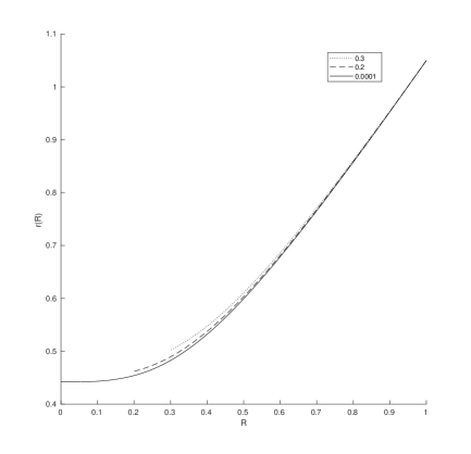
(a) $r_{\varepsilon}$

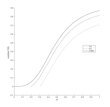
(b) $\hat{T}(r_{\varepsilon}(\cdot))$

Figure 1: Computed minimizers of $\hat{I}_{\varepsilon}$ when $\lambda=1.05$ and $\varepsilon=0.3,0.2,10^{-4}$.

For these values, the critical boundary displacement is $\lambda_{c}\approx 1.0258$ (cf. [15]). For $\varepsilon=0.3,0.2,10^{-4}$ and $\lambda=1.05$ (case $\lambda>\lambda_{c}$) we show in Figure 1 the computed solutions $r_{\varepsilon}$ and the modified Cauchy stress functions $\hat{T}(r_{\varepsilon}(\cdot))$, the former converging very nicely to a cavitating solution while the later to a well defined increasing function vanishing at $R=0$. The cavity size for the computed solution with $\varepsilon=10^{-4}$ is $0.44184$ approximately with modified energy of $1.2774$. The affine deformation in this case has energy of $1.2888$.

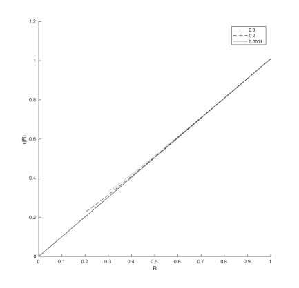
(a) $r_{\varepsilon}$

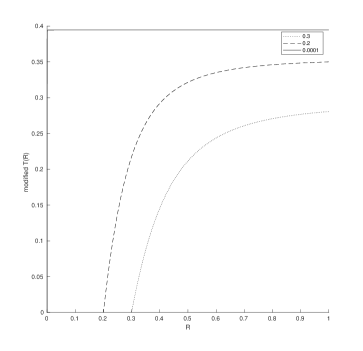
(b) $\hat{T}(r_{\varepsilon}(\cdot))$

Figure 2: Computed minimizers $r_{\varepsilon}$ and modified Cauchy stress functions $\hat{T}(r_{\varepsilon}(\cdot))$ for $\hat{I}_{\varepsilon}$ when $\lambda=1.01$ and $\varepsilon=0.2,0.1,0.05,10^{-4}$.

For $\lambda=1.01$ which corresponds to the case $\bar{\lambda}<\lambda<\lambda_{c}$, as $\bar{\lambda}=1$, we show in Figure 2 the computed $r_{\varepsilon}$ and $\hat{T}(r_{\varepsilon}(\cdot))$. The convergence is now to the affine deformation $r_{h}(R)=1.01R$ with energy of $1.2733$. The corresponding Cauchy stress functions show sharp boundary layers at $R=\varepsilon$ while converging pointwise to a positive constant function.

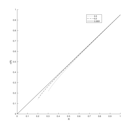
(a) $r_{\varepsilon}$

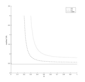
(b) $\hat{T}(r_{\varepsilon}(\cdot))$

Figure 3: Computed minimizers $r_{\varepsilon}$ and modified Cauchy stress functions $\hat{T}(r_{\varepsilon}(\cdot))$ for $\hat{I}_{\varepsilon}$ when $\lambda=0.95$ and $\varepsilon=0.2,0.1,0.05,10^{-4}$.

The other calculation we show is for $\lambda=0.95$ (case $\lambda<\bar{\lambda}=1$) with the same values of $\varepsilon$. The results are presented in Figure 3 where we can clearly see the convergence of the $r_{\varepsilon}$ to the affine deformation $r_{h}(R)=0.95R$ with energy of $1.3625$ (Figure 3a). The $r_{\varepsilon}$’s in this figure are concave functions corresponding to the case where $\dot{v}>0$ in (51). On the other hand in Figure 3b we see the corresponding Cauchy stress functions converging pointwise, with a sharp boundary layer at $R=\varepsilon$, to a negative constant function.

Example 5.2.

In this example we study the so called incompressible limit by considering a sequence of compressible problems formally approaching an incompressible one. In particular we consider functions $h(\cdot)$ in (39) given by

$$h(d)=C\,\left(d-1-\frac{1}{C}\right)^{2}+D\,d^{-\delta},$$

where $C,D\geq 0$ and $\delta>0$. As $C\rightarrow\infty$ we formally approach the incompressible modified stored energy function given by:

$$\hat{\Phi}^{inc}(v_{2},\ldots,v_{n})=\frac{\kappa}{n}\,(v_{2}\cdots v_{n})^{-n}+D+\kappa\left(\frac{n-1}{n}+\ln(v_{2}\cdots v_{n})\right),$$

For the computations we used the following:

$$n=3,\quad\kappa=3,\quad D=1.5,\quad\delta=2,$$

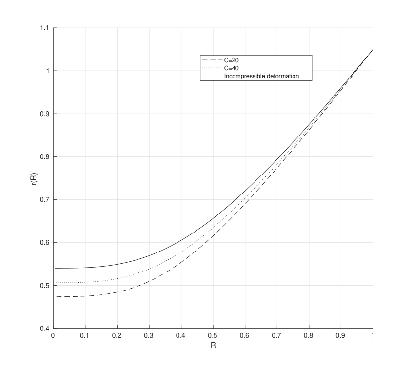
Figure 4: Minimizers of modified compressible problems approaching the incompressible deformation in the incompressible limit with $C$ increasing.

with $\lambda=1.05$. In Figure 4 we show in solid the solution of the incompressible problem which is given by $r_{inc}(R)=\sqrt[3]{R^{3}+\lambda^{3}-1}$, together with the computed minimizers of the modified compressible problems (48) with $\varepsilon=0.005$ and $C=20,40$ (dashed and dotted respectively), which are clearly seen getting close to $r_{inc}$. We computed as well solutions of the modified compressible problems for additional values of $C$ together with their modified energies. The results are shown in Table 1. The energy of $r_{inc}$, computed using $\hat{\Phi}^{inc}$ above, is given approximately by $1.53013$. Thus we see as well a nice convergence of the energies of the modified compressible problems in the incompressible limit.

Table 1: Energies for the modified compressible problems in the incompressible limit case.

$C$	$\hat{I}_{\varepsilon}(r_{\varepsilon})$	$C$	$\hat{I}_{\varepsilon}(r_{\varepsilon})$
20	1.52298	160	1.52864
40	1.52532	320	1.52936
80	1.52735	640	1.52974

6 Concluding Remarks

It is not difficult to check that the results of this paper can be generalized to stored energy functions of the form

$$W(\mathbf{F})=\frac{\kappa}{n}\left\|\mathbf{F}\right\|^{n}+h(\det\mathbf{F})=\frac{\kappa}{n}(v_{1}^{2}+\cdots+v_{n}^{2})^{\frac{n}{2}}+h(v_{1}\cdots v_{n}).$$ (52)

In fact, an analysis for this stored energy function similar to the one leading to Proposition 2.2, shows that $T(v)$ is now asymptotic to $-\kappa(n-1)^{n/2}\ln(v)$ as $v\rightarrow\infty$. Thus we are led to consider a modified functional of the form

$$\hat{I}(r) = \int_{0}^{1}R^{n-1}\Bigg{[}\frac{\kappa}{n}\left(\left[r^{\prime}(R)^{2}+(n-1)\left(\frac{r}{R}\right)^{2}\right]^{\frac{n}{2}}-(n-1)^{\frac{n}{2}}\left(\frac{r}{R}\right)^{n}\right)$$

$$+h\left(\delta(R)\right)+\kappa(n-1)^{\frac{n}{2}}\delta(R)\left(\frac{1}{n}+\ln\left(\frac{r}{R}\right)\right)\Bigg{]}\,\mathrm{d}R-\frac{\kappa(n-1)^{\frac{n}{2}}}{n}\lambda^{n}\ln\lambda.$$

As this functional can be characterised in terms of the original one plus suitable null Lagrangians, its Euler–Lagrange equation coincides with that of the original functional. The rest of the analysis in this paper should now follow through.

The radial incompressible case can be treated similarly to the compressible case studied in this paper. However, the incompressible case is more straightforward since a radial incompressible deformation of the form (12) which also satisfies (5) is necessarily given by

$$r(R)=(R^{n}+(\lambda^{3}-1))^{\frac{1}{n}},$$

for $\lambda>1$. On using this form, [1, Prop. 5.1] shows that

$$-\int_{\lambda}^{b}\frac{1}{v^{n}-1}\frac{\mathrm{d}}{\mathrm{d}v}\Phi(v^{1-n},v,\ldots,v)\,\mathrm{d}v+n\int_{\lambda}^{b}\frac{v^{n-1}}{(v^{n}-1)^{2}}\Phi(v^{1-n},v,\ldots,v)\,\mathrm{d}v$$

$$~{}~{}~{}~{}~{}~{}~{}~{}~{}~{}~{}~{}~{}~{}~{}~{}~{}~{}~{}~{}~{}~{}~{}~{}~{}~{}~{}~{}~{}~{}~{}~{}~{}~{}~{}=\frac{1}{\lambda^{n}-1}\Phi(\lambda^{1-n},\lambda,\ldots,\lambda),$$

for any $b>\lambda$ (the case $b$ finite corresponds to integrating over a punctured ball in the reference configuration of internal radius $\left(\frac{\lambda^{n}-1}{b^{n}-1}\right)^{\frac{1}{n}}$. As $b\rightarrow\infty$ (corresponding to the puncture closing up), the first term on the left of this equation is, up to a constant, the radial Cauchy stress (on the deformed puncture surface) whilst the second term is the $n$ times the energy of the deformed punctured ball. Taking the form of $\Phi$ in this incompressible case as $(\kappa/n)\sum_{i=1}^{n}v_{i}^{n}$ plus some constant, it is easy to obtain from the expression above that the growth in the radial Cauchy stress is once again asymptotically proportional to $\ln(b)$ as $b\rightarrow\infty$.

In generalising the techniques in this paper from radially symmetric deformations to none radial ones, one approach (cf. [22]) is to restrict attention to deformations for which the distributional determinant of the deformation satisfies:

$$\mbox{Det}(\nabla{\mathbf{u}})=(\det\nabla{\mathbf{u}})\mathcal{L}^{n}+V_{\mathbf{u}}\delta_{\mathbf{0}},$$

where $\delta_{\mathbf{0}}$ is the Dirac measure supported at the origin and $V_{\mathbf{u}}$ is the volume of the cavity formed by the deformation ${\mathbf{u}}$ at the origin. From [21, Proposition 3.6] we get that in the case $n=3$,

$$\int_{\mathcal{B}_{\varepsilon}}\left\|\nabla\mathbf{u}\right\|^{3}\,\mathrm{d}\mathbf{x}\geq\int_{\mathcal{B}_{\varepsilon}}\left\|\nabla\mathbf{u}^{\mbox{rad}}\right\|^{3}\,\mathrm{d}\mathbf{x}\geq-2^{\frac{3}{2}}\,\omega_{3}\,\tilde{r}^{3}(\varepsilon)\ln(\varepsilon),$$ (53)

where $\omega_{3}=4\pi$. Here $\mathbf{u}^{\mbox{rad}}$ is the radial symmetrization of $\mathbf{u}$ and is given by (12) where $r$ is replaced by $\tilde{r}$ which in turn is given by

$$\frac{4\pi}{3}\,\tilde{r}^{3}(R)=\frac{4\pi}{3}\,\lambda^{3}-\int_{\mathcal{B}_{R}}\det(\nabla\mathbf{u})\,\mathrm{d}\mathbf{x}.$$

(The inequality (53) holds provided $\tilde{r}^{\prime}(R)\leq\tilde{r}(R)/R$ for all $R\in[\varepsilon,1]$. If this condition is not satisfied, then the symmetrisation $\tilde{r}$ has to be modified as in [22] in order for (53) to hold.) Thus, it should follow from (53) that the total energy due to the deformation $\mathbf{u}$ blows up at least like $-\ln(\varepsilon)$ as $\varepsilon\rightarrow 0^{+}$ if $V_{\mathbf{u}}>0$. Thus, in generalizing our results to the non–radial case with the stored energy function (52), we are led to consider a modified energy functional given by

$$\hat{E}(\mathbf{u})=\lim_{\varepsilon\rightarrow 0}\left[\int_{\mathcal{B}_{\varepsilon}}W(\nabla{\mathbf{u}})\,\mathrm{d}\mathbf{x}+2^{\frac{3}{2}}\kappa\,V_{{\mathbf{u}}}\ln(\varepsilon)\right].$$

It may now follow from the approach in [21] that, for each $\varepsilon>0$, the minimizer of the functional in brackets above (over $\mathcal{B}_{\varepsilon}$) must be radial. Under suitable hypotheses, it may then follow that the minimizer of $\hat{E}$ is radial and so the results of the current paper would then be applicable. We shall pursue these ideas elsewhere.

References

• [1] J. M. Ball, Discontinuous Equilibrium Solutions and Cavitation in Nonlinear Elasticity, Phil. Trans. Royal Soc. London A 306, 557-611, 1982.
• [2] F. Béthuel, H. Brezis, and F. Hélein, Ginzburg–Landau vortices, Progress in Nonlinear Differential Equations and Their Applications, 13. Birkh auser, Boston, 1994.
• [3] V. Cañulef-Aguilar and D. Henao, A lower bound for the void coalescence load in nonlinearly elastic solids, Interfaces And Free Boundaries, Vol. 21, Issue 4, pp. 409–440, 2019.
• [4] J. D. Eshelby, The force on an elastic singularity, Proc. R. Soc. A244, 87–111, 1951.
• [5] A. N. Gent and P. B. Lindley, Internal rupture of bonded rubber cylinders in tension, Proc. R. Soc. Lond. A 249, pp. 195–205, 1958.
• [6] S. Govindjee and P. A. Mihalic, Computational methods for inverse finite elastostatics, Comput. Methods Appl. Mech. Engrg., 136, 47–57, 1996.
• [7] A. E. Green, On some general formulae in finite elastostatics, Arch. Rational Mech. Anal. 50, pp. 73-80, 1973.
• [8] D. Henao and C. Mora-Corral, Invertibility and weakcontinuity of the determinant for the modelling of cavitation and fracture in nonlinear elasticity, Arch. Rat. Mech. Anal., 197 (2010), pp. 619–655.
• [9] D. Henao and S. Serfaty, Energy estimates and cavity interaction for a critical-exponent cavitation model, Communications on Pure and Applied Mathematics, Vol. LXVI, 1028–1101, 2013.
• [10] D. Henao and R. Rodiac, On the existence of minimizers for the neo-Hookean energy in the axisymmetric setting, Discrete Contin. Dyn. Syst., 38, 4509–4536, 2018.
• [11] C. O. Horgan and D. A. Polignone, Cavitation in nonlinearly elastic solids: A review, Appl. Mech. Rev. 48 (1995), pp. 471–485.
• [12] R. James and S. J. Spector, The formation of filamentary voids in solids, J. Mech. Phys. Solids 39 (1991), pp. 783–813.
• [13] F. Meynard, Existence and nonexistence results on the radially symmetric cavitation problem, Quart. Appl. Math. 50 (1992), pp. 201–226.
• [14] S. Müller and S. J. Spector, An existence theory for nonlinear elasticity that allows for cavitation, Arch. Rat. Mech. Anal., 131 (1995), pp. 1–66.
• [15] P. V. Negrón–Marrero and J. Sivaloganathan, The Numerical Computation of the Critical Boundary Displacement for Radial Cavitation, Mathematics and Mechanics of Solids, 14: 696-726, 2009.
• [16] J. W. Neuberger, Sobolev Gradients and Differential Equations, Lecture Notes in Math. 1670, Springer, Berlin, 1997.
• [17] T. J. Pence and K. Gou, On compressible versions of the incompressible neo-Hookean material, Mathematics and Mechanics of Solids, Vol. 20(2) 157–182, 2015.
• [18] J. Sivaloganathan, Uniqueness of regular and singular equilibria for spherically symmetric problems of nonlinear elasticity, Arch. Rat. Mech. Anal., 96, 97–136, 1986.
• [19] J. Sivaloganathan and S. J. Spector, On the existence of minimizers with prescribed singular points in nonlinear elasticity, J. Elasticity, 59 (2000), pp. 83–113.
• [20] J. Sivaloganathan and S. J. Spector, On the optimal location of singularities arising in variational problems of elasticity, Journal of Elasticity, 58, 191–224, 2000.
• [21] J. Sivaloganathan and S. J. Spector., On the symmetry of energy minimizing deformations in nonlinear elasticity II: compressible materials, Arch. Rational Mech. Anal, Vol. 196, 395–431, 2010.
• [22] J. Sivaloganathan, S. J. Spector, and V. Tilakraj, The convergence of regularized minimizers for cavitation problems in nonlinear elasticity, SIAM J. Appl. Math, 66, 736-757, 2006.
• [23] C. A. Stuart, Radially symmetric cavitation for hyperelastic materials, Analyse non lineaire, 2, 33–66, 1985.
• [24] C. A. Stuart, Estimating the critical radius for radially symmetric cavitation, Quarterly of Applied Mathematics, Vol LI, 251-263, 1993.
• [25] S. K. Vodop’yanov, V. M. Gol’dshtein. and Yu. G. Reshetnyak, The geometric properties of functions with generalized first derivatives. Russian Math. Surveys, 34:19–74, 1979.
Refer to caption