Supervised Multivariate Learning with Simultaneous
Feature Auto-grouping and Dimension Reduction

Abstract

Modern high-dimensional methods often adopt the “bet on sparsity” principle, while in supervised multivariate learning statisticians may face “dense” problems with a large number of nonzero coefficients. This paper proposes a novel clustered reduced-rank learning (CRL) framework that imposes two joint matrix regularizations to automatically group the features in constructing predictive factors. CRL is more interpretable than low-rank modeling and relaxes the stringent sparsity assumption in variable selection. In this paper, new information-theoretical limits are presented to reveal the intrinsic cost of seeking for clusters, as well as the blessing from dimensionality in multivariate learning. Moreover, an efficient optimization algorithm is developed, which performs subspace learning and clustering with guaranteed convergence. The obtained fixed-point estimators, though not necessarily globally optimal, enjoy the desired statistical accuracy beyond the standard likelihood setup under some regularity conditions. Moreover, a new kind of information criterion, as well as its scale-free form, is proposed for cluster and rank selection, and has a rigorous theoretical support without assuming an infinite sample size. Extensive simulations and real-data experiments demonstrate the statistical accuracy and interpretability of the proposed method.

1 Introduction

Modern statistical applications create an urgent need for analyzing and interpreting high-dimensional data with low-dimensional structures. This paper works in a supervised multivariate setting with $n$ samples for $m$ responses and $p$ features (or predictors): $\boldsymbol{Y}=[\boldsymbol{y}_{1},\ldots,\boldsymbol{y}_{m}]\in\mathbb{R}^{n\times m}$ and $\boldsymbol{X}=[\boldsymbol{x}_{1},\ldots,\boldsymbol{x}_{p}]\in\mathbb{R}^{n\times p}$. Given a loss $l_{0}$, not necessarily a negative log-likelihood function, one can solve the following optimization problem to model the set of responses of interest

$$\min_{\boldsymbol{B}\in\mathbb{R}^{p\times m}}l_{0}(\boldsymbol{X}\boldsymbol{B};\boldsymbol{Y}).$$ (1)

Here, the unknown coefficient matrix $\boldsymbol{B}=[\boldsymbol{b}_{1},\ldots,\boldsymbol{b}_{p}]^{T}$ has $pm$ unknowns, with $\boldsymbol{b}_{j}$ summarizing the contributions of the $j$-th predictor to all the responses.

The modern-day challenge comes from large $p$ and/or $m$. Statisticians often prefer selecting a small subset of features—for example, a group-$\ell_{1}$ penalty $\lambda\sum\|\boldsymbol{b}_{j}\|_{2}$ (Yuan and Lin,, 2006) can be added in the criterion to promote row-wise sparsity in $\boldsymbol{B}$, which results in a more interpretable model than using an $\ell_{2}$-type penalty $\lambda\|\boldsymbol{B}\|_{F}^{2}$. However, with a large $m$, there may exist few features that are completely irrelevant to the whole set of responses. One may perform variable selection in a transformed space rather than the original space (Johnstone and Lu,, 2009), but how to find a proper transformation to reveal sparsity is problem-specific.

Perhaps a natural alternative is to make the coefficients form a relatively small number of groups, within each of which all coefficients are forced to be equal. This is referred to as “equisparsity” in She, (2010). In the general multivariate setup, instead of requiring a large number of zero rows in the true signal $\boldsymbol{B}^{*}$, we assume that it has relatively few distinct row patterns $\boldsymbol{b}_{(1)}^{*T},\boldsymbol{b}_{(2)}^{*T},\ldots,\boldsymbol{b}_{(q)}^{*T}$. Then, from

$$\boldsymbol{X}\boldsymbol{B}^{*}=\boldsymbol{x}_{1}\boldsymbol{b}_{1}^{*T}+\cdots+\boldsymbol{x}_{p}\boldsymbol{b}_{p}^{*T}=\big{(}\sum_{j\in\mathcal{G}_{1}}\boldsymbol{x}_{j}\big{)}\boldsymbol{b}_{(1)}^{*T}+\cdots+\big{(}\sum_{j\in\mathcal{G}_{q}}\boldsymbol{x}_{j}\big{)}\boldsymbol{b}_{(q)}^{*T},$$ (2)

the features sharing the same $\boldsymbol{b}_{(k)}^{*}$ ($1\leq k\leq q$) are automatically grouped, based on their contributions to $\boldsymbol{Y}$. The feature grouping is as interpretable as feature selection and can offer further parsimony, since the latter only targets the set of irrelevant features with $\boldsymbol{b}_{j}^{*}=\boldsymbol{0}$.

The problem of how to cluster the unknown coefficient matrix to achieve the best predictability falls into supervised learning, where both $\boldsymbol{Y}$ and $\boldsymbol{X}$ are available. This is in contrast to conventional clustering tasks for unsupervised learning that operate on a single data matrix. But it shares the same computational challenge in large dimensions. A nice but sometimes unnoticed fact is that if $p$ points form $q$ clusters in a large $m$-dimensional vector space, then the clusters can be revealed in just a $q$-dimensional subspace, such as the one spanned by the cluster centroids. In real data analysis, it is not rare that the dimension of the cluster centroid space is much less than $q$ (even as low as 2 or 3). This motivates us to perform simultaneous dimension reduction to ease the job of clustering.

Specifically, we propose to including an additional low-rank constraint, and the resulting jointly regularized form provides an extension of the celebrated reduced rank regression (RRR, Izenman, (1975)). RRR assumes that the rank of the true $\boldsymbol{B}^{*}$ is no more than a small number $r$, or equivalently, $\boldsymbol{B}^{*}=\boldsymbol{B}_{1}\boldsymbol{B}_{2}^{T}$ with each $\boldsymbol{B}_{i}$ having $r$ columns. Once locating a proper loading matrix $\boldsymbol{B}_{1}$, the final model amounts to fitting $\boldsymbol{Y}$ on $r$ factors formed by $\boldsymbol{X}\boldsymbol{B}_{1}$. Unfortunately, it is well known that the factor construction from a large number of features lacks interpretability. Our proposal of clustered rank reduction enforces row-wise equisparsity in $\boldsymbol{B}_{1}$ (or the overall coefficient matrix) so that in extracting $r$ predictive factors, the original features can be automatically consolidated into $q$ groups at the same time.

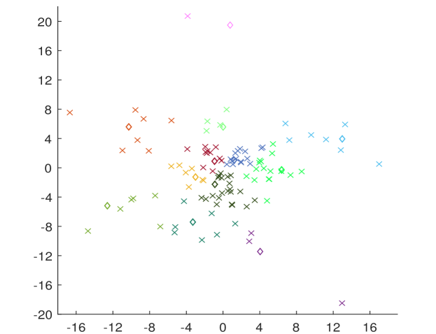
Figure 1: Yeast cell cycle data: the loading weights, denoted by ‘$\times$’, by fitting an RRR with $r=2$. The many noticeable nonzeros imply that a number of TFs have effects on the gene expressions during the cell cycle process. Here, the 12 diamonds represent the consolidated loadings obtained by the proposed CRL method.

It is perhaps best to illustrate the idea on a real-world example. The yeast cell cycle data used in Chun and Keleş, (2010) studies transcription factors (TFs) related to gene expression over time. In addition to the predictor matrix $\boldsymbol{X}\in\mathbb{R}^{542\times 106}$ with $106$ TFs collected on $542$ genes, a response matrix $\boldsymbol{Y}\in\mathbb{R}^{542\times 18}$ containing RNA levels measured on the same genes is available at $18$ time points. A naive multivariate regression would have about 2k unknowns, and so we fit an RRR with $r=2$ and plot the loadings of the 106 TFs in Figure 1. The fact that most of the loadings are apparently nonzero makes variable selection less effective in reducing the complexity of the model. Indeed, because of the high-quality experimental design by biologists, quite a few TFs seem to have effects on the gene expressions during the cell cycle process.

Intuitively, clustering the TFs’ loadings would offer a significant reduction of the number of free parameters. Note that to enhance interpretability and avoid ad-hoc tuning, we force the estimates within a group to be equal. A stagewise procedure performing estimation and clustering in two distinct steps would be suboptimal; we aim to solve the problem as a whole. The diamonds in Figure 1 show the loadings obtained by the proposed method that simultaneously groups the features in performing dimension reduction.

Compared with the low-rank modeling, the new parsimonious model not only boosted the prediction accuracy by 23% (over 200 repeated training-test splits with 50% for training and 50% for test), but offered some meaningful TF groups. For example, that ACE2, SWI5 and SOK2 fall into the same group and share the same set of large coefficients provides useful biological insights, as it is well known that ACE2 and SWI5 are paralogs, meaning that they are related to each other through a gene duplication event and are highly conserved in yeast cell cycle gene progression, and according to Pan and Heitman, (2000), with regards to nitrogen limitation, SOK2, along with ACE2 and SWI5, is essential in the pseudohyphal growth of yeast cells. Our analysis also provides a cluster with three TFs, namely HIR1, STP2 and SWI4, all of which are chromatin-associated transcription factors involved in regulating the expression of multiple genes at distinct phases of yeast cells (Lambert et al.,, 2010).

This paper studies simultaneous feature auto-grouping and dimension reduction, and attempts to tackle some related challenges in methodology, theory, and computation. Our main contributions are as follows.

• A novel clustered reduced-rank learning (CRL) framework is proposed, which imposes joint matrix regularizations through a convenient SV formulation. It relaxes the assumption of sparsity and offers improved interpretability compared with vanilla low-rank modeling. The concurrent dimension reduction substantially eases the task of clustering in high dimensions.

• Universal information-theoretical limits reveal the intrinsic cost of seeking for clusters, as well as the benefit of accumulating a large number of responses in multivariate learning, which seems to be largely unknown in the literature before.

• Tight error bounds are shown for CRL beyond the standard likelihood setup and justify its minimax optimality in some common scenarios. These nonasymptotic results are strikingly different from those for sparse learning and are the first of their kind. Our theoretical studies favor CRL over variable selection when the numbers of relevant features and irrelevant features are of the same order, or when the number of responses is greater than or equal to the number of features up to a multiplicative constant.

• An efficient optimization-based algorithm is developed, which performs simultaneous subspace pursuit and clustering with guaranteed convergence. The resulting fixed-point estimators, though not necessarily globally optimal, achieve the desired statistical accuracy under some regularity conditions.

• A predictive information criterion is proposed for joint cluster and/or rank selection. Its brand new model complexity notion differs from existing information criteria, but has a rigorous theoretical support in finite samples. A scale-free form is further proposed to bypass the noise scale estimation.
  

The rest of the paper is organized as follows. Section 2 describes in detail the clustered reduced-rank learning framework to automatically group the predictors in building a predictive low-rank model. Section 3 shows some universal minimax lower bounds and tight upper bounds of CRL, from which one can conclude that CRL enjoys minimax optimality if the number of clusters is at most polynomially large in the rank. The obtained rates differ substantially from the standard results assuming sparsity, and interestingly, having a large number of responses seems to be a blessing. Section 4 develops an iterative and easy-to-implement algorithm by linearization and block coordinate descent, where Procrustes rotations and clusterings are performed repeatedly with guaranteed convergence. A new predictive information criterion, together with its scale-free form, is proposed for model selection in the context of clustered rank reduction. Section 5 shows some real data analysis. We conclude in Section 6. The appendices provide all technical details and more computer experiments.

Notation and symbols. The following notation and symbols will be used. Given a differentiable $f$, we use $\nabla f$ to denote its gradient, and $f$ is called $\mu$-strongly convex if $f({\boldsymbol{\eta}}^{\prime})\geq f({\boldsymbol{\eta}})+\langle\nabla f({\boldsymbol{\eta}}),{\boldsymbol{\eta}}^{\prime}-{\boldsymbol{\eta}}\rangle+\mu\|{\boldsymbol{\eta}}^{\prime}-{\boldsymbol{\eta}}\|_{2}^{2}/2,\forall{\boldsymbol{\eta}},{\boldsymbol{\eta}}^{\prime},$ and $L$-strongly smooth if $f({\boldsymbol{\eta}}^{\prime})\leq f({\boldsymbol{\eta}})+\langle\nabla f({\boldsymbol{\eta}}),{\boldsymbol{\eta}}^{\prime}-{\boldsymbol{\eta}}\rangle+L\|{\boldsymbol{\eta}}^{\prime}-{\boldsymbol{\eta}}\|_{2}^{2}/2,\ \forall{\boldsymbol{\eta}},{\boldsymbol{\eta}}^{\prime}.$ In particular, $f({\boldsymbol{\eta}})=\|{\boldsymbol{\eta}}-\boldsymbol{y}\|_{2}^{2}/2$ is 1-strongly convex. For any $\boldsymbol{A},\boldsymbol{B}\in\mathbb{R}^{n\times m}$, we denote by $\langle\boldsymbol{A},\boldsymbol{B}\rangle$ the inner product of $\boldsymbol{A},\boldsymbol{B}$. Given $\boldsymbol{A}\in\mathbb{R}^{n\times m}$, $\boldsymbol{A}^{+}$ denotes its Moore-Penrose inverse, $\mathrm{rank}(\boldsymbol{A})$ denotes its rank, and when $n=m$, $\sigma_{\max}(\boldsymbol{A})$ denotes its maximal eigenvalue. We use $\boldsymbol{A}[i,j]$ to represent the $(i,j)$-th element in $\boldsymbol{A}$ and $\boldsymbol{A}[i,:]$ (or $\boldsymbol{A}[:,i]$) to represent the $i$-th row (or column) of $\boldsymbol{A}$. Some conventional matrix norms of $\boldsymbol{A}$ are as follows: $\|\boldsymbol{A}\|_{F}$ denotes the Frobenius norm, $\|\boldsymbol{A}\|_{2}$ the spectral norm, $\|\boldsymbol{A}\|_{*}$ the nuclear norm, and $\|\boldsymbol{A}\|_{2,\infty}=\max_{1\leq j\leq p}\|\boldsymbol{a}_{j}\|_{2}$ for $\boldsymbol{A}=[\boldsymbol{a}_{1},\ldots,\boldsymbol{a}_{p}]^{T}$. The constants denoted by $C$, $c$ are not necessarily the same at each occurrence. Finally, $a\lesssim b$ means $a\leq cb$ up to a multiplicative positive constant $c$, and $a\asymp b$ means $a\lesssim b$ and $b\lesssim a$.

2 Clustered Reduced Rank Regression

This section focuses on the quadratic loss commonly used in multivariate regression,

$$l_{0}(\boldsymbol{X}\boldsymbol{B};\boldsymbol{Y})=\|\boldsymbol{Y}-\boldsymbol{X}\boldsymbol{B}\|_{F}^{2}/2.$$

The discussions in this important case will lay out a foundation for computation and theoretical analysis in later sections regarding a general loss.

Motivated by Section 1, rather than assuming that most features are irrelevant to the responses, we propose to enforce row-wise equisparsity in $\boldsymbol{B}$ so that we can group the features in modeling $\boldsymbol{Y}$. Sparsity is just a special case of equisparsity, and clustering the nonzero values can gain further parsimony. Meanwhile, we would like to regularize the multivariate model with low rank, making it possible to project the data into a much smaller subspace to reveal the row patterns of $\boldsymbol{B}$.

To mathematically formulate the problem, we use $\|\boldsymbol{b}\|_{\mathcal{C}}$ to denote the number of distinct elements in vector $\boldsymbol{b}$, and $\|\boldsymbol{B}\|_{2,\mathcal{C}}$ the number of distinct rows of $\boldsymbol{B}$. Then, our clustered reduced-rank learning (CRL) involves the minimization of the loss criterion with two constraints $\mathrm{rank}(\boldsymbol{B})\leq r,\|\boldsymbol{B}\|_{2,\mathcal{C}}\leq q$. The joint regularization formulation poses significant challenges in both computation and theory.

A trick to decouple the two intertwined constraints is to write $\boldsymbol{B}=\boldsymbol{S}\boldsymbol{V}^{T}$ with $\boldsymbol{V}$ an $m\times r$ column-orthogonal matrix. The “SV” formulation will be used in optimization as well. Since $\boldsymbol{S}=\boldsymbol{B}\boldsymbol{V}$, we get $\|\boldsymbol{S}\|_{2,\mathcal{C}}=\|\boldsymbol{B}\|_{2,\mathcal{C}}$ and thus an equivalent CRL problem with separate constraints on $\boldsymbol{S}$ and $\boldsymbol{V}$:

$$\min_{\boldsymbol{S}\in\mathbb{R}^{p\times r},\boldsymbol{V}\in\mathbb{R}^{m\times r}}\|\boldsymbol{Y}-\boldsymbol{X}\boldsymbol{S}\boldsymbol{V}^{T}\|_{F}^{2}\quad\mbox{s.t.}\,\ \ \boldsymbol{V}^{T}\boldsymbol{V}=\boldsymbol{I},\ \|\boldsymbol{S}\|_{2,\mathcal{C}}\leq q.$$ (3)

In (3), $q$ ($1\leq q\leq p$) controls the number of feature groups, and $r$ ($r\leq m$) is the dimension of the subspace to pursue coefficient clustering. The joint tuning of the regularization parameters $q$ and $r$ is an important task, too, and a data-adaptive solution with theoretical support will be given in Section 4.2. Let $\boldsymbol{V}=[\boldsymbol{v}_{1},\ldots,\boldsymbol{v}_{r}]$ and $\boldsymbol{S}=[\boldsymbol{s}_{1},\ldots,\boldsymbol{s}_{r}]$. We call $\boldsymbol{s}_{i}\ (1\leq i\leq r)$ the clustering vectors. An intercept term $\boldsymbol{1}\boldsymbol{\alpha}^{T}$ can be added to the loss to help control the scale of clustering vectors. Equivalently, for regression, one can simply center $\boldsymbol{Y},\boldsymbol{X}$ columnwise in advance. We also suggest standardizing the predictors beforehand, as done in other regularization methods like LASSO and ridge regression, unless all the predictors are on the same scale.

We discuss a special case of (3) to provide a more intuitive understanding on the mathematical problem, which can also be used to develop a sequential estimation procedure. Letting $r=1$, (3) becomes $\min_{\boldsymbol{s}\in\mathbb{R}^{p},\boldsymbol{v}\in\mathbb{R}^{m}}\|\boldsymbol{Y}-\boldsymbol{X}\boldsymbol{s}\boldsymbol{v}^{T}\|_{F}^{2}\mbox{ s.t. }\|\boldsymbol{v}\|_{2}^{2}=1,\|\boldsymbol{s}\|_{\mathcal{C}}\leq q$. Reparematrize $\boldsymbol{s}=d\boldsymbol{s}^{\circ}$ with $d\in\mathbb{R}$ and $\boldsymbol{s}^{\circ}$ satisfying $\|\boldsymbol{X}\boldsymbol{s}^{\circ}\|_{2}=1$. Simple algebra shows that the problem is minimized at $d=\langle\boldsymbol{X}\boldsymbol{s}^{\circ}\boldsymbol{v}^{T},\boldsymbol{Y}\rangle$ and $\boldsymbol{v}=\boldsymbol{Y}^{T}\boldsymbol{X}\boldsymbol{s}^{\circ}/\|\boldsymbol{Y}^{T}\boldsymbol{X}\boldsymbol{s}^{\circ}\|_{2}$. Therefore, (3) reduces to (4) when $r=1$:

$$\max_{\boldsymbol{s}^{\circ}\in{\mathbb{R}}^{p}}{\boldsymbol{s}^{\circ}}^{T}(\boldsymbol{X}^{T}{\boldsymbol{Y}\boldsymbol{Y}^{T}}\boldsymbol{X})\boldsymbol{s}^{\circ}\ \ \mbox{ s.t. }\ \boldsymbol{s}^{\circ T}\boldsymbol{X}^{T}\boldsymbol{X}\boldsymbol{s}^{\circ}=1,\|\boldsymbol{s}^{\circ}\|_{\mathcal{C}}\leq q.$$ (4)

Without the last constraint, (4) is a generalized eigenvalue decomposition problem. The regularization enforces equisparsity in estimating the generalized eigenvector. Though (4) is intuitive, (3) is much more amenable to optimization.

The regularization admits other variants via the SV-formulation. For example, with $\boldsymbol{B}=\boldsymbol{S}\boldsymbol{V}^{T}=\boldsymbol{s}_{1}\boldsymbol{v}_{1}^{T}+\cdots+\boldsymbol{s}_{r}\boldsymbol{v}_{r}^{T}$, one can pursue equisparsity in each component $\boldsymbol{s}_{i}\boldsymbol{v}_{i}^{T}$ or $\boldsymbol{s}_{i}$:

$$\min_{\boldsymbol{S}\in\mathbb{R}^{p\times r},\boldsymbol{V}\in\mathbb{R}^{m\times r}}\|\boldsymbol{Y}-\boldsymbol{X}\boldsymbol{S}\boldsymbol{V}^{T}\|_{F}^{2}\quad\mbox{s.t.}\ \ \boldsymbol{V}^{T}\boldsymbol{V}=\boldsymbol{I},\ \|\boldsymbol{s}_{i}\|_{\mathcal{C}}\leq q^{e},\ 1\leq i\leq r.$$ (5)

This rankwise CRL allows each feature to belong to more than one cluster as $r>1$. In comparison, the constraint in (3) offers a uniform control. Unless otherwise mentioned, we will focus on the row-wise problem (3), but our algorithm applies to both.

Remark 1.

Alternative formulations of CRL. Given a positive definite matrix $\boldsymbol{\Gamma}$ of size $m\times m$, consider a weighted criterion: $\min_{(\boldsymbol{S},\boldsymbol{V})\in\mathbb{R}^{p\times r}\times\mathbb{R}^{m\times r}}\allowbreak\mbox{Tr}\{(\boldsymbol{Y}-\boldsymbol{X}\boldsymbol{S}\boldsymbol{V}^{T})\boldsymbol{\Gamma}(\boldsymbol{Y}-\boldsymbol{X}\boldsymbol{S}\boldsymbol{V}^{T})^{T}\}\mbox{ s.t. }\boldsymbol{V}^{T}\boldsymbol{V}=\boldsymbol{I},\|\boldsymbol{S}\|_{{2,C}}\leq q.$ Then, for $\boldsymbol{B}=\boldsymbol{S}\boldsymbol{V}^{T}\boldsymbol{\Gamma}^{{1}/{2}}$, we have $\mathrm{rank}(\boldsymbol{B})\leq r$ and $\|\boldsymbol{B}\|_{2,C}=\|\boldsymbol{S}\|_{2,C}$. Applying the SV representation to $\boldsymbol{B}$ gives an equivalent problem (with $\boldsymbol{S},\boldsymbol{V}$ redefined)

$$\min_{(\boldsymbol{S},\boldsymbol{V})\,\in\,\mathbb{R}^{p\times r}\times\mathbb{R}^{m\times r}}\frac{1}{2}\|\boldsymbol{Y}\boldsymbol{\Gamma}^{{1}/{2}}-\boldsymbol{X}\boldsymbol{S}\boldsymbol{V}^{T}\|_{F}^{2}\ \mbox{ s.t. }\ \boldsymbol{V}^{T}\boldsymbol{V}=\boldsymbol{I},\|\boldsymbol{S}\|_{2,C}\leq q.$$ (6)

(6) is of the same form of (3) with an adjusted response matrix.

Another related projected form directly measures discrepancy in the projected space:

$$\min_{(\boldsymbol{S},\boldsymbol{A})\,\in\,\mathbb{R}^{p\times r}\times\mathbb{R}^{m\times r}}\frac{1}{2}\|\boldsymbol{Y}\boldsymbol{A}-\boldsymbol{X}\boldsymbol{S}\|_{F}^{2}\mbox{ s.t. }(\boldsymbol{Y}\boldsymbol{A})^{T}\boldsymbol{Y}\boldsymbol{A}=n\boldsymbol{I},\|\boldsymbol{S}\|_{2,\mathcal{C}}\leq q,$$ (7)

where we assume $r\leq\mathrm{rank}(\boldsymbol{Y})$. Let $\boldsymbol{\Sigma}_{Y}=\boldsymbol{Y}^{T}\boldsymbol{Y}/n=\boldsymbol{U}\boldsymbol{D}\boldsymbol{U}^{T}$ with the diagonal matrix $\boldsymbol{D}$ containing $\mathrm{rank}(\boldsymbol{Y})$ nonzero eigenvalues, $\boldsymbol{W}=\boldsymbol{D}^{1/2}\boldsymbol{U}^{T}\boldsymbol{A}$, and $\boldsymbol{B}=\boldsymbol{S}\boldsymbol{W}^{T}\boldsymbol{D}^{1/2}\boldsymbol{U}^{T}$. Because $\|\boldsymbol{Y}\boldsymbol{A}-\boldsymbol{X}\boldsymbol{S}\|_{F}^{2}=\mbox{Tr}\{(\boldsymbol{Y}-\boldsymbol{X}\boldsymbol{B})\boldsymbol{\Sigma}_{Y}^{+}(\boldsymbol{Y}-\boldsymbol{X}\boldsymbol{B})^{T}\}+nr-n\mathrm{rank}(\boldsymbol{Y})$ (cf. Lemma A.8), $\mathrm{rank}(\boldsymbol{B})\leq r$, and $\boldsymbol{B}$, $\boldsymbol{S}$ have the same row patterns, we see that the projected form simply amounts to taking $\boldsymbol{\Gamma}=\boldsymbol{\Sigma}_{Y}^{+}$. Popular choices of $\boldsymbol{\Gamma}$ are based on the covariance matrix of $\boldsymbol{Y}$. See She et al., (2020) for a proposal to account for dependence in the case of a general loss. A further topic is to estimate the high-dimensional covariance matrix and mean matrix jointly, but it is beyond the scope of the current paper and we regard $\boldsymbol{\Gamma}$ as known. Then, based on (6), one simply needs to “whiten” $\boldsymbol{Y}$ by $\boldsymbol{Y}\boldsymbol{\Gamma}^{\frac{1}{2}}$ beforehand.

Remark 2.

Pairwise-difference penalization. An alternative idea, following She, (2010) and Chi and Lange, (2015), is to penalize the pairwise row-differences of $\boldsymbol{B}=[\boldsymbol{b}_{1},\ldots,\boldsymbol{b}_{p}]^{T}$:

$$\sum_{1\leq j<j^{\prime}\leq p}P(\|\boldsymbol{b}_{j}-\boldsymbol{b}_{j^{\prime}}\|_{2};\lambda),$$

where $P$ is a sparsity-inducing function. This type of regularization is however not of our primary interest, due to its computational burden, suboptimal error rate, and difficulties in parameter tuning. See Appendix A.5 and Theorem A.3 for more details.

Remark 3.

Unsupervised learning. Supervised learning is the focus of our work, but when there is a single data matrix $\boldsymbol{Y}\in\mathbb{R}^{n\times m}$, we can set $\boldsymbol{X}=\boldsymbol{I}$ in (3) to cluster its rows for unsupervised learning. (Substituting $\boldsymbol{Y}^{T}$ for $\boldsymbol{Y}$ offers clustered PCA as an alternative to sparse PCA.) Similar to the derivation in the rank-1 case, we can evaluate the optimal $\boldsymbol{V}$ to get $\min_{\boldsymbol{S}\in\mathbb{R}^{n\times r}}\|\boldsymbol{S}\|_{F}^{2}/2-\|\boldsymbol{Y}^{T}\boldsymbol{S}\|_{*}$ s.t. $\|\boldsymbol{S}\|_{2,\mathcal{C}}\leq q$, or $\max_{\|\boldsymbol{S}^{\circ}\|_{F}=1}\|\boldsymbol{Y}^{T}\boldsymbol{S}^{\circ}\|_{*}^{2}/2$ s.t. $\|\boldsymbol{S}^{\circ}\|_{2,\mathcal{C}}\leq q$ via $\boldsymbol{S}=d\boldsymbol{S}^{\circ}$. (In the more general supervised setup, we can show that $\boldsymbol{S}$ solves $\min_{\boldsymbol{S}\in\mathbb{R}^{p\times r}}\allowbreak\|\boldsymbol{X}\boldsymbol{S}\|_{F}^{2}/2-\|\boldsymbol{Y}^{T}\boldsymbol{X}\boldsymbol{S}\|_{*}$ s.t. $\|\boldsymbol{S}\|_{2,\mathcal{C}}\leq q$.) Because $\|\boldsymbol{Y}^{T}\boldsymbol{S}\|_{*}=\mbox{Tr}\{(\boldsymbol{S}^{T}\boldsymbol{Y}\boldsymbol{Y}^{T}\boldsymbol{S})^{1/2}\}$, CRL’s clustering vectors depend on $\boldsymbol{Y}$ through its sample inner products only. One can then introduce a kernel CRL by substituting a positive semi-definite $\boldsymbol{K}$ for $\boldsymbol{Y}\boldsymbol{Y}^{T}$. The desired clusters can still be obtained by solving the SV-form problem, with a suitable pseudo-response constructed from the kernel matrix. Let’s consider two special cases to contrast the unsupervised CRL with some related methods. (a) No data projection, i.e., $r=m$. Then we can show that K-means is an algorithm to solve the problem (cf. Section 4.1). Modern implementations of K-means make good use of seeding and can obtain a decent solution in low dimensions, which will assist the optimization of CRL, owing to its low-rank nature. Of course, as K-means operates in the input space, it can be ineffective for large $m$. (b) No equisparsity regularization. In this case, CRL reduces to spectral clustering (cf. Appendix B.1). Giving up the equisparsity regularization simplifies the computation significantly, but spectral clustering, as well as other similarity-motivated procedures, performs dimension reduction and clustering in two distinct steps. It would be less greedy to perform both steps simultaneously. In Section 4, we will see that the CRL algorithm can integrate clustering and subspace learning to solve the problem as a whole.

3 Nonasymptotic Statistical Analysis of Clustered Reduced-rank Learning

Rigorous theoretical guarantees must be provided to justify the proposed clustered rank reduction method. There is a big literature gap to fill in this regard. For example, how many samples are needed for signal recovery by adopting the new notion of structural parsimony? In which situations will pursuing equisparsity be advantageous over performing variable selection? Is it always necessary to obtain a globally optimal solution in the nonconvex setup? The answers to these questions seem to be largely unknown.

In this section, we go beyond the regression setup and consider a loss $l_{0}(\boldsymbol{X}\boldsymbol{B};\boldsymbol{Y})$ that is defined on the systematic component $\boldsymbol{X}\boldsymbol{B}$ with $\boldsymbol{Y}$ as parameters. Here, $\boldsymbol{B}$ is unknown and $\boldsymbol{X}$ and $\boldsymbol{Y}$ are observed, and so we occasionally omit the dependence on $\boldsymbol{Y}$. Assume that $l_{0}$ is differentiable with respect to $\boldsymbol{X}\boldsymbol{B}$. Our tool for tackling a general loss is the generalized Bregman function (She et al.,, 2021): given a differentiable function $\psi$,

$${\mathbf{\Delta}}_{\psi}(\boldsymbol{\alpha},\boldsymbol{\beta}):=\psi(\boldsymbol{\alpha})-\psi(\boldsymbol{\beta})-\langle\nabla\psi(\boldsymbol{\beta}),\boldsymbol{\alpha}-\boldsymbol{\beta}\rangle.$$ (8)

If $\psi$ is also strictly convex, ${\mathbf{\Delta}}_{\psi}(\boldsymbol{\alpha},\boldsymbol{\beta})$ becomes the standard Bregman divergence denoted by $\mathbf{D}_{\psi}(\boldsymbol{\alpha},\boldsymbol{\beta})$ (Bregman,, 1967). A simple example is ${\mathbf{D}}_{2}(\boldsymbol{\alpha},\boldsymbol{\beta}):=\|\boldsymbol{\alpha}-\boldsymbol{\beta}\|_{2}^{2}/2$, associated with $\psi=\|\,\cdot\,\|_{2}^{2}/2$, and its matrix version is ${\mathbf{D}}_{2}(\boldsymbol{A},\boldsymbol{B})=\|\operatorname{\mbox{vec}\,}(\boldsymbol{A})-\operatorname{\mbox{vec}\,}(\boldsymbol{B})\|_{2}^{2}/2=\|\boldsymbol{A}-\boldsymbol{B}\|_{F}^{2}/2$. In general, ${\mathbf{\Delta}}_{\psi}(\boldsymbol{\alpha},\boldsymbol{\beta})$ may not be symmetric, and we define its symmetrized version by $\bar{\boldsymbol{\Delta}}_{\psi}(\boldsymbol{\alpha},\boldsymbol{\beta}):=(\boldsymbol{\Delta}_{\psi}(\boldsymbol{\alpha},\boldsymbol{\beta})+\boldsymbol{\Delta}_{\psi}(\boldsymbol{\beta},\boldsymbol{\alpha}))/2.$

Introducing the notion of noise in the non-likelihood setup is another essential component, since $l_{0}$ may not correspond to a distribution function. We define the effective noise associated with the statistical truth $\boldsymbol{B}^{*}$ by

$$\boldsymbol{E}=-\nabla l_{0}(\boldsymbol{X}\boldsymbol{B}^{*};\boldsymbol{Y}).$$ (9)

So having a zero-mean noise means that the risk vanishes at the statistical truth, assuming we can exchange the gradient and expectation. In a canonical generalized linear model (GLM) with cumulant function $b(\cdot)$ and $g=(\nabla b)^{-1}$ as the canonical link (cf. Appendix A), the (unscaled) loss can be represented by $-\langle\boldsymbol{Y},\boldsymbol{X}\boldsymbol{B}\rangle+b(\boldsymbol{X}\boldsymbol{B})$, and by matrix differentiation,

$$\boldsymbol{E}=\boldsymbol{Y}-g^{-1}(\boldsymbol{X}\boldsymbol{B}^{*})=\boldsymbol{Y}-\mathbb{E}(\boldsymbol{Y}),$$

or $\boldsymbol{E}=\boldsymbol{Y}-\boldsymbol{X}\boldsymbol{B}^{*}$ in regression. Unless otherwise specified, we assume that $\operatorname{\mbox{vec}\,}(\boldsymbol{E})$ is a sub-Gaussian random vector with mean zero and scale bounded by $\sigma$ (namely, all marginals $\langle\operatorname{\mbox{vec}\,}(\boldsymbol{E}),\boldsymbol{\alpha}\rangle$ satisfy $\|\langle\operatorname{\mbox{vec}\,}(\boldsymbol{E}),\boldsymbol{\alpha}\rangle\|_{\psi_{2}}\leq\sigma\|\boldsymbol{\alpha}\|_{2}$, $\forall\boldsymbol{\alpha}\in\mathbb{R}^{p}$, where $\|\cdot\|_{\psi_{2}}=\inf\big{\{}t>0:\,\mathbb{E}\exp[(\cdot\,/{t})^{2}]\leq 2\big{\}},$ cf. van der Vaart and Wellner, (1996)). Note that the components of $\boldsymbol{E}$ need not be independent. Sub-Gaussian noises are typical in regression and classification problems, since Gaussian and bounded random variables are sub-Gaussian. Yet sub-Gaussianity is not critical for our analysis.

This section focuses on row-wise equisparsity $\|\boldsymbol{B}\|_{2,\mathcal{C}}$. It turns out that the two measures $\|\cdot\|_{2,\mathcal{C}}$ and $\mathrm{rank}(\cdot)$ can effectively bound the stochastic terms arising from CRL. Because it is be difficult in present-day applications to tell whether the sample size, relative to the problem dimensions, is large enough to apply asymptotics, all of our investigations will be nonasymptotic.

3.1 Universal minimax lower bounds

The first question one must answer is how small the error could be under equisparsity with possibly low rank. We derive new minimax lower bounds to address the question. Let $I(\cdot)$ be an arbitrary nondecreasing function with $I(0)=0,I\not\equiv 0$; some particular examples are $I(t)=t$ and $I(t)=1_{t\geq c}$.

Theorem 1.

Assume $\boldsymbol{Y}|\boldsymbol{X}\boldsymbol{B}^{*}$ follows a distribution in the regular exponential family with dispersion $\sigma^{2}$ with $l_{0}$ the associated negative log-likelihood function (cf. Appendix A for details). Define a signal class by

$$\boldsymbol{B}^{*}\in\mathcal{S}(q,r)=\{\boldsymbol{B}\in\mathbb{R}^{p\times m}:\|\boldsymbol{B}\|_{2,\mathcal{C}}\leq q,\,\mathrm{rank}(\boldsymbol{B})\leq r\},$$ (10)

where $p\geq q\geq r\geq 2$, $r(q\wedge\mathrm{rank}(\boldsymbol{X})+m-r)\geq 4$. Let $b,\zeta$ be any integers satisfying

$$\sum_{i=0}^{\zeta}{r\choose i}(b-1)^{i}\geq q,$$ (11)

with $b\geq 2,1\leq\zeta\leq r$, and define a complexity function

$$P(q,r)=(q+m)r+p\,\{\log(er)-\log\log q\}.$$ (12)

Assume for some $\kappa>0$

$${\mathbf{\Delta}}_{l_{0}}(\boldsymbol{0},\boldsymbol{X}\boldsymbol{B})\sigma^{2}\allowbreak\leq\kappa\|\boldsymbol{B}\|_{F}^{2}/2,\ \ \forall\boldsymbol{B}\in\mathcal{S}(q,r).$$ (13)

Then there exist positive constants $c,c^{\prime}$, depending on $I(\cdot)$ only, such that

$$\inf_{\hat{\boldsymbol{B}}}\sup_{\boldsymbol{B}^{*}\in\mathcal{S}(q,r)}\,\mathbb{E}\left\{I\Big{(}\|\boldsymbol{B}^{*}-\hat{\boldsymbol{B}}\|_{F}^{2}{\big{/}}\Big{[}c\sigma^{2}\big{\{}(q+m)r+\frac{p\log q}{b^{2}\zeta}\big{\}}/\kappa\Big{]}\Big{)}\right\}\geq c^{\prime}>0,$$ (14)

where $\hat{\boldsymbol{B}}$ denotes an arbitrary estimator. In particular, under $8\leq q\leq\exp(r)$,

$$\inf_{\hat{\boldsymbol{B}}}\,\sup_{\boldsymbol{B}^{*}\in\mathcal{S}(q,r)}\mathbb{E}\big{[}I\big{(}\|\boldsymbol{B}^{*}-\hat{\boldsymbol{B}}\|_{F}^{2}/\{c\sigma^{2}P(q,r)/\kappa\}\big{)}\big{]}\geq c^{\prime}>0.$$ (15)

A more complete theorem including minimax lower bounds for both the estimation error $\|\hat{\boldsymbol{B}}-\boldsymbol{B}^{*}\|_{F}$ and prediction error $\|\boldsymbol{X}\hat{\boldsymbol{B}}-\boldsymbol{X}\boldsymbol{B}^{*}\|_{F}$ is presented in Appendix A.1, from which one can see that the size of $\phi:=q^{1/r}$ plays a vital role in determining the final error rate. These results are the first of their kind and provide useful guidance in the context of equisparsity. Our proof is nontrivial and makes use of $q$-ary codes in information theory (Pellikaan et al.,, 2017), as well as some useful facts of the generalized Bregman functions for GLMs.

The regularity condition (13) is not restrictive. For regression and logistic regression, the condition is implied by ${\mathbf{\Delta}}_{l_{0}}(\boldsymbol{0},\boldsymbol{X}\boldsymbol{B})\sigma^{2}\allowbreak\leq\|\boldsymbol{X}\boldsymbol{B}\|_{F}^{2}/2$ and ${\mathbf{\Delta}}_{l_{0}}(\boldsymbol{0},\boldsymbol{X}\boldsymbol{B})\leq\|\boldsymbol{X}\boldsymbol{B}\|_{F}^{2}/8$, respectively. The bound in (14) is general, while (15) is perhaps more illustrative: when $q\leq\exp(r)$ and $\kappa\leq cn$,

$$\,\mathbb{E}\big{[}\|\boldsymbol{B}^{*}-\hat{\boldsymbol{B}}\|_{F}^{2}\big{]}\geq c\sigma^{2}P(q,r)/n,\mbox{ and }\,\mathbb{P}\big{[}\|\boldsymbol{B}^{*}-\hat{\boldsymbol{B}}\|_{F}^{2}\geq c\sigma^{2}P(q,r)/n\big{]}>c_{0}>0,$$

by setting $I(t)=t$ and $I(t)=1_{t\geq c}$, respectively. Therefore, in the scenario of $q$ being polynomially large in $r$, i.e., $q\leq r^{c}$ for some constant $c$, no estimator can beat the error rate $P(q,r)\asymp(q+m)r+p\log q$ in a minimax sense. Interestingly, when $m$ is a constant, the rate reduction compared to $pm$ is not significant, whereas having a large number of response variables is (perhaps surprisingly) a blessing for pursuing equisparsity.

3.2 Upper error bounds of CRL

Can we approach the optimal error rate using a particular estimator? This part shows that CRL is a legitimate method, and more importantly, pursuing its globally optimal solutions is unnecessary in many cases. Rather, finding a fixed point of CRL, defined by (16) and (17) below, would suffice for regular problems.

Let $r^{*}=\mathrm{rank}(\boldsymbol{B}^{*})$ and $q^{*}=\|\boldsymbol{B}^{*}\|_{2,\mathcal{C}}$. Given a differentiable $l_{0}$, define

$$G_{\rho}(\boldsymbol{B};\boldsymbol{B}^{-})=l_{0}(\boldsymbol{X}\boldsymbol{B};\boldsymbol{Y})-{\mathbf{\Delta}}_{l_{0}}(\boldsymbol{X}\boldsymbol{B},\boldsymbol{X}\boldsymbol{B}^{-})+{\rho}{\mathbf{D}}_{2}(\boldsymbol{B},\boldsymbol{B}^{-}),$$ (16)

where $\rho$, representing the inverse stepsize, is an algorithm parameter to be chosen. Then, for all fixed points defined by

$$\hat{\boldsymbol{B}}\in\operatorname*{argmin}_{\boldsymbol{B}:\|\boldsymbol{B}\|_{2,\mathcal{C}}\leq q,\mathrm{rank}(\boldsymbol{B})\leq r}G_{\rho}(\boldsymbol{B};\boldsymbol{B}^{-})|_{\boldsymbol{B}^{-}=\hat{\boldsymbol{B}}},$$ (17)

a nonasymptotic error bound can be derived by calculating the metric entropy of the associated manifolds and using the Stirling numbers of the second kind.

Theorem 2.

Let $r\geq r^{*}$, $q\geq q^{*}$, and $\hat{\boldsymbol{B}}$ be any fixed point satisfying (17) for some $\rho>0$. Define

$$P_{o}(q,r)=\{q\wedge\mathrm{rank}(\boldsymbol{X})+m\}r+(p-q)\log q.$$ (18)

Assume $\rho>0$ is chosen so that

$$\rho{\mathbf{D}}_{2}(\boldsymbol{B}_{1},\boldsymbol{B}_{2})\leq(2\bar{\mathbf{\Delta}}_{l_{0}}-\delta{\mathbf{D}}_{2})(\boldsymbol{X}\boldsymbol{B}_{1},\boldsymbol{X}\boldsymbol{B}_{2})+K\sigma^{2}P_{o}(q,r),\ \forall\boldsymbol{B}_{i}:\mathrm{rank}(\boldsymbol{B}_{i})\leq r,\|\boldsymbol{B}_{i}\|_{2,\mathcal{C}}\leq q$$ (19)

for some $\delta>0$ and sufficiently large $K\geq 0$. Then, $\hat{\boldsymbol{B}}$ satisfies

$$\,\mathbb{E}[\|\boldsymbol{X}\hat{\boldsymbol{B}}-\boldsymbol{X}\boldsymbol{B}^{*}\|_{F}^{2}]\lesssim\frac{K\delta\vee 1}{\delta^{2}}\big{\{}\sigma^{2}(q\wedge\mathrm{rank}(\boldsymbol{X})+m)r+\sigma^{2}(p-q)\log q+\sigma^{2}\big{\}}.$$ (20)

It is not difficult to see that when $l_{0}$ is $\mu$-strongly convex, the following matrix restricted eigenvalue condition implies (19) with $K=0$:

$$\rho\|\boldsymbol{B}_{1}-\boldsymbol{B}_{2}\|_{F}^{2}\leq(2\mu-\delta)\|\boldsymbol{X}(\boldsymbol{B}_{1}-\boldsymbol{B}_{2})\|_{F}^{2},\quad\forall\boldsymbol{B}_{i}:\mathrm{rank}(\boldsymbol{B}_{i})\leq r,\|\boldsymbol{B}_{i}\|_{2,\mathcal{C}}\leq q.$$ (21)

When $q$ is small, (21) is applicable to large-$p$ designs. Similar regularity conditions are widely used in compressed sensing, variable selection and low rank estimation (Candès and Tao,, 2007; Bickel et al.,, 2009; Candès and Plan,, 2011).

Let $q=\vartheta q^{*}$, $r=\vartheta r^{*}$ with $\vartheta\geq 1$. When $\vartheta$, $\delta$ and $K$ are treated as constants and $\sigma=1$, from (20), the prediction error bound is of the order

$$\{q^{*}\wedge\mathrm{rank}(\boldsymbol{X})+m\}r^{*}+(p-q^{*})\log q^{*},$$ (22)

ignoring all trivial multiplicative/additive terms. The rate distinguishes CRL from various sparse learning methods in the literature.

Remark 4.

Computational feasibility. The fact that the fixed-point solutions, though not necessarily globally or even locally optimal, can have provable guarantees offers a feasible computation of the nonconvex CRL optimization problem in regular cases.

Specifically, regardless of the choice of the loss, $G_{\rho}$ always has a simple quadratic form in terms of $\boldsymbol{B}$, which gives rise to an iterative update of the coefficient matrix. Similar results can be shown for $(\boldsymbol{S},\boldsymbol{V})$ obtained by alternative optimization; see Theorem A.2 in Remark 8. Section 4.1 designs an efficient algorithm on the basis of linearization and block coordinate descent.

Remark 5.

Error rate comparison. To clarify the theoretical meaning of (22), we make an error-rate comparison between CRL and some commonly used estimators in regression with $\sigma=1$ (assuming all regularity conditions are met). First, assuming that $\boldsymbol{X}$ has full column rank, the ordinary least squares has $\,\mathbb{E}\|\boldsymbol{X}\hat{\boldsymbol{B}}-\boldsymbol{X}\boldsymbol{B}^{*}\|_{F}^{2}=mp$. With no rank reduction ($r^{*}=q^{*}$), (22) gives $(q^{*}+m)q^{*}+(p-q^{*})\log q^{*}$, which is $\lesssim mp$ when the number of responses is larger than the number of feature groups. Of course, if $r^{*}<q^{*}$, CRL can achieve a much lower error rate. Comparing (22) with $(p+m)r^{*}$ by low-rank matrix estimation (Bunea et al.,, 2011), we see that CRL does a substantially better job if the number of clusters does not grow exponentially with the rank, namely, $q^{*}\ll\exp(r^{*})$.

Variable selection gives another important means of regularization. If $\boldsymbol{B}^{*}=[\boldsymbol{b}_{1}^{*},\ldots,\boldsymbol{b}_{p}^{*}]^{T}$ is row-wise sparse with $s^{*}=|\{j:\boldsymbol{b}_{j}^{*}\neq\boldsymbol{0}\}|$, the prediction error by means of variable selection is of the order (Lounici et al.,, 2011)

$$s^{*}m+s^{*}\log p.$$ (23)

The comparison between (23) and (22) shows no clear winner: for the degrees-of-freedom terms, $(\mathrm{rank}(\boldsymbol{X})\wedge q^{*}+m)r^{*}\leq q^{*}r^{*}+ms^{*}\lesssim s^{*}m$, while for the ‘inflation’ terms, $(p-q^{*})\log q^{*}$ is typically larger than $s^{*}\log p$. But two scenarios draw our particular attention:

$$\mbox{ (i) ``many responses'': }m\geq cp\qquad\mbox{ (ii) ``linear sparsity'': }s^{*}=cp$$

where $c$ is a positive constant. In either situation, CRL is advantageous over variable selection.

Concretely, in case (i), $s^{*}m+s^{*}\log p\asymp s^{*}m$, while from $s^{*}\geq q^{*}\geq r^{*}$, we have $s^{*}m\geq r^{*}m\geq r^{*}q^{*}$ and $s^{*}m\gg(\log q^{*})(p-q^{*})$, and so $s^{*}m+s^{*}\log p\gtrsim\{q^{*}\wedge\mathrm{rank}(\boldsymbol{X})+m\}r^{*}+(p-q^{*})\log q^{*}$. In case (ii), $s^{*}\log p\asymp p\log p\geq(p-q^{*})\log q^{*}$ and the same conclusion holds. In other words, when the number of responses is greater than the number of features up to a multiplicative constant, or when the number of relevant features and the number of irrelevant features are of the same order, CRL has a lower error rate with rigorous theoretical support.

Remark 6.

Minimax optimality. One may be curious if the upper error bound of CRL could match the universal minimax lower bound. Notably, under the mild conditions $q^{*}\leq\mathrm{rank}(\boldsymbol{X})$ and $q^{*}\ll\exp(r^{*})$ (and so $q^{*}\log q^{*}\ll q^{*}r^{*}$), (22) becomes

$$(q^{*}+m)r^{*}+p\log q^{*},$$

which is exactly the rate shown at the end of in Section 3.1. So at least for canonical GLMs with $q^{*}$ polynomially large in $r^{*}$, CRL does enjoy minimax rate optimality.

Of course, the previous discussions assume that $q$ and $r$ are specified so that they are not too large relative to $q^{*}$ and $r^{*}$, respectively. In general, the data-adaptive tuning to be introduced in Section 4.2 still ensures (22).

To the best of our knowledge, Theorem 3 is the first nonasymptotic statistical analysis of the set of CRL’s fixed points in nonconvex optimization. One might ask whether the error rate can be further improved by pursuing a global CRL estimator. The following theorem shows that this is not the case, but the regularity condition (19) gets relaxed to some extent.

Theorem 3.

Let $\hat{\boldsymbol{B}}$ be an optimal CRL solution with $r\geq r^{*}$ and $q\geq q^{*}$. Assume that there exists some $\delta>0$ such that

$${\mathbf{\Delta}}_{l_{0}}(\boldsymbol{X}\boldsymbol{B}_{1},\boldsymbol{X}\boldsymbol{B}_{2})\geq\delta{\mathbf{D}}_{2}(\boldsymbol{X}\boldsymbol{B}_{1},\boldsymbol{X}\boldsymbol{B}_{2}),\ \forall\boldsymbol{B}_{i}:\|\boldsymbol{B}_{i}\|_{2,\mathcal{C}}\leq q,\mathrm{rank}(\boldsymbol{B}_{i})\leq r.$$ (24)

Then $\,\mathbb{E}[\|\boldsymbol{X}\hat{\boldsymbol{B}}-\boldsymbol{X}\boldsymbol{B}^{*}\|_{F}^{2}]\lesssim\frac{1}{\delta^{2}}\{\sigma^{2}(q\wedge\mathrm{rank}(\boldsymbol{X})+m)r+\sigma^{2}(p-q)\log q+\sigma^{2}\}$.

Unlike (19) in Theorem 2, (24) uses ${{\mathbf{\Delta}}}_{l_{0}}$ (in place of twice of its symmetrized version) and does not involve $\rho$. The conclusion of Theorem 3 can be extended to an oracle inequality (Donoho and Johnstone,, 1994), and these $\ell_{2}$-recovery results can be used to give some estimation error bounds under proper regularity conditions. Corollary 1 gives an illustration.

Corollary 1.

Let $l_{0}$ be $\mu$-strongly convex. Then for any $\boldsymbol{B}:\mathrm{rank}(\boldsymbol{B})\leq r,\|\boldsymbol{B}\|_{2,\mathcal{C}}\leq q$,

$$\,\mathbb{E}{\mathbf{D}}_{l_{0}}(\boldsymbol{X}\hat{\boldsymbol{B}},\boldsymbol{X}\boldsymbol{B}^{*})\|_{F}^{2}\lesssim\,\mathbb{E}{\mathbf{D}}_{l_{0}}(\boldsymbol{X}\boldsymbol{B},\boldsymbol{X}\boldsymbol{B}^{*})+\frac{\sigma^{2}}{\mu}\{(q\wedge\mathrm{rank}(\boldsymbol{X})+m)r+(p-q)\log q\}+\frac{\sigma^{2}}{\mu}.$$ (25)

Furthermore, assume $\|\boldsymbol{X}\boldsymbol{B}\|_{F}^{2}/n\geq\delta\|\boldsymbol{B}\|_{2,\infty}^{2},\forall\boldsymbol{B}:\mathrm{rank}(\boldsymbol{B})\leq(1+\vartheta)r^{*},\|\boldsymbol{B}\|_{2,\mathcal{C}}\leq\vartheta q^{*2}$ for some $\delta>0$, and $r=\vartheta r^{*},q=\vartheta q^{*}$, $\vartheta\geq 1$, $q^{*}>1$. Then with probability at least $1-C\exp\{-c(m+\mathrm{rank}(\boldsymbol{X}))\}$,

$$\|\hat{\boldsymbol{B}}-\boldsymbol{B}^{*}\|_{2,\infty}^{2}\leq\frac{c_{0}\vartheta^{2}\sigma^{2}}{n\delta\mu^{2}}\{(q^{*}\wedge\mathrm{rank}(\boldsymbol{X})+m)r^{*}+(p-q^{*})\log q^{*}\}$$ (26)

for some constants $c_{0},c,C>0$.

The RHS of (25) offers a bias-variance tradeoff and as a result, CRL applies to $\boldsymbol{B}^{*}$ with just approximate equisparsity and/or low rank. The $(2,\infty)$-norm error bound (26) implies faithful cluster recovery with high probability, if the signal-to-noise ratio is properly large: $\min_{b_{j\cdot}^{*}\neq b_{k\cdot}^{*}}\allowbreak|\mbox{avg}_{l}{b_{jl}^{*2}}-\mbox{avg}_{l}b_{kl}^{*2}|/\sigma^{2}>2\zeta$. Here, $\mbox{avg}_{l}{b_{jl}^{*2}}$ is the average of $b_{j1}^{*2},\ldots,b_{jm}^{*2}$ and $\zeta=\frac{c_{0}\vartheta^{2}}{\delta\mu^{2}}\{\frac{(p-q^{*})\log q^{*}}{nm}+\frac{r^{*}(q^{*}\wedge\mathrm{rank}(\boldsymbol{X}))}{nm}+\frac{r^{*}}{n}\}.$ Then, from the bound on $\|\hat{\boldsymbol{B}}-\boldsymbol{B}^{*}\|_{2,\infty}^{2}$, we know that for $q=q^{*}$, $\hat{\boldsymbol{B}}$ exhibits the same row clusters as does $\boldsymbol{B}^{*}$, and for $q>q^{*}$, $\hat{\boldsymbol{B}}$ refines the clustering structure of $\boldsymbol{B}^{*}$.

4 Computation and Tuning

In this section, we develop an efficient optimization-based CRL algorithm with implementation ease and guaranteed convergence. We also propose a novel model comparison criterion and provide its theoretical justification from a predictive learning perspective, without assuming any infinite sample-size or large signal-to-noise ratio conditions.

4.1 Algorithm design

In this part, we discuss how to solve the CRL problem with $q$ and $r$ fixed. CRL poses some intriguing challenges in optimization: the problem is highly nonconvex, $l_{0}$ is not restricted to the quadratic loss or a negative log-likelihood function, and the equisparsity and low-rank constraints are of discrete nature. These obstacles render standard algorithms inapplicable. In addition, as $p$ and $m$ may be large in real applications, the coefficient matrix $\boldsymbol{B}\in\mathbb{R}^{p\times m}$ can easily contain an overwhelming number of unknowns. Then, how to make use of its low-rank nature to reduce the computational cost at each iteration, while maintaining the convergence of the overall procedure, is crucial in large-scale computation.

Before describing the algorithm design in full detail, we provide below a simplified version of the algorithm.

Algorithm 1 Clustered Reduced-rank Learning Algorithm

0:  $(\boldsymbol{Y},\boldsymbol{X})\in\mathbb{R}^{n\times m}\times\mathbb{R}^{n\times p}$, $l_{0}$: a loss function with $\nabla l_{0}$ $L$-Lipschitz continuous; $q$: desired number of clusters; $\epsilon$: error tolerance; $M$: maximum number of iterations; a feasible starting point: $\boldsymbol{F}^{0},{\boldsymbol{\mu}}^{0},\boldsymbol{V}^{[0]}$, $\boldsymbol{\alpha}^{[0]}$; $\rho$: inverse stepsize (e.g., $L\|\boldsymbol{X}\|_{2}^{2}$)

1:  $k\leftarrow 0$, $\boldsymbol{S}^{[0]}=\boldsymbol{F}^{0}{\boldsymbol{\mu}}^{0}$;

2:  while $k<M$ and $\epsilon<\|\boldsymbol{B}^{[k]}-\boldsymbol{B}^{[k-1]}\|\mbox{ (if existing)}$  do

3:     $k\leftarrow k+1$;

4:     $\boldsymbol{B}^{[k-1]}=\boldsymbol{S}^{[k-1]}(\boldsymbol{V}^{[k-1]})^{T}$,  $\widetilde{\boldsymbol{Y}}\leftarrow\boldsymbol{B}^{[k-1]}-\boldsymbol{X}^{T}\nabla l_{0}(\boldsymbol{1}\boldsymbol{\alpha}^{[k-1]}+\boldsymbol{X}\boldsymbol{B}^{[k-1]})/\rho$;

5:     $\boldsymbol{\alpha}^{[k]}\leftarrow\boldsymbol{\alpha}^{[k-1]}-[\nabla l_{0}(\boldsymbol{1}\boldsymbol{\alpha}^{[k-1]}+\boldsymbol{X}\boldsymbol{B}^{[k-1]})]^{T}\boldsymbol{1}/\rho$;

6:     $t\leftarrow 0,\boldsymbol{S}^{(0)}\leftarrow\boldsymbol{S}^{[k-1]},\boldsymbol{V}^{(0)}\leftarrow\boldsymbol{V}^{[k-1]},\boldsymbol{B}^{(0)}\leftarrow\boldsymbol{S}^{(0)}\boldsymbol{V}^{(0)T}$;

7:     while not converged do

8:        $t\leftarrow t+1$;

9:        $\boldsymbol{W}\leftarrow\widetilde{\boldsymbol{Y}}^{T}\boldsymbol{S}^{(t-1)}$;

10:        $\boldsymbol{V}^{(t)}\leftarrow\boldsymbol{U}_{w}\boldsymbol{V}^{T}_{w}$ with $\boldsymbol{U}_{w}$, $\boldsymbol{V}_{w}$ from the SVD $\boldsymbol{W}=\boldsymbol{U}_{w}\boldsymbol{D}_{w}\boldsymbol{V}_{w}^{T}$;

11:        $\boldsymbol{L}\leftarrow\widetilde{\boldsymbol{Y}}\boldsymbol{V}^{(t)}$;

12:        With ${\boldsymbol{\mu}}^{0}$ as the initial cluster centroid matrix, call K-means on $\boldsymbol{L}$ to update $\boldsymbol{F}^{l}$ and ${\boldsymbol{\mu}}^{l}\,(l\geq 1)$ alternatively till convergence;

13:        $\boldsymbol{S}^{(t)}\leftarrow\boldsymbol{F}^{l}{\boldsymbol{\mu}}^{l}$, $\boldsymbol{B}^{(t)}=\boldsymbol{S}^{(t)}(\boldsymbol{V}^{(t)})^{T}$, ${\boldsymbol{\mu}}^{0}\leftarrow{\boldsymbol{\mu}}^{l}$;

14:     end while

15:     $\boldsymbol{S}^{[k]}\leftarrow\boldsymbol{S}^{(t)},\boldsymbol{V}^{[k]}\leftarrow\boldsymbol{V}^{(t)},\boldsymbol{B}^{[k]}\leftarrow\boldsymbol{S}^{[k]}(\boldsymbol{V}^{[k]})^{T}$;

16:  end while

17:  return  $\boldsymbol{S}=\boldsymbol{S}^{[k]},\boldsymbol{V}=\boldsymbol{V}^{[k]},\boldsymbol{F}=\boldsymbol{F}^{l}$.

Define $\iota_{\boldsymbol{V}}(\boldsymbol{V})=0$ if $\boldsymbol{V}^{T}\boldsymbol{V}=\boldsymbol{I}$ and $+\infty$ otherwise. Similarly, $\iota_{2,\mathcal{C}}(\boldsymbol{S})=0$ if $\|\boldsymbol{S}\|_{2,\mathcal{C}}\leq q$ and $+\infty$ otherwise, and $\iota_{\mathcal{C}}(\boldsymbol{S})=0$ if $\|\boldsymbol{s}_{i}\|_{\mathcal{C}}\leq q^{e}$ for all $1\leq i\leq r$ and $+\infty$ otherwise. We use $\iota(\boldsymbol{S})$ to denote $\iota_{2,\mathcal{C}}(\boldsymbol{S})$ in the row-equisparsity case and $\iota_{\mathcal{C}}(\boldsymbol{S})$ in the rankwise case. The loss $l_{0}(\boldsymbol{X}\boldsymbol{B};\boldsymbol{Y})$ is also written as $l_{0}(\boldsymbol{X}\boldsymbol{S}\boldsymbol{V}^{T};\boldsymbol{Y})$ or $l(\boldsymbol{S},\boldsymbol{V};\boldsymbol{X},\boldsymbol{Y})$, often abbreviated as $l_{0}(\boldsymbol{X}\boldsymbol{S}\boldsymbol{V}^{T})$ or $l(\boldsymbol{S},\boldsymbol{V})$ for convenience. The general CRL optimization problem can be stated as

$$\min_{\boldsymbol{S}\in\mathbb{R}^{p\times r},\boldsymbol{V}\in\mathbb{R}^{m\times r}}f(\boldsymbol{S},\boldsymbol{V}):=l(\boldsymbol{S},\boldsymbol{V};\boldsymbol{X},\boldsymbol{Y})+\iota(\boldsymbol{S})+\iota_{\boldsymbol{V}}(\boldsymbol{V}).$$ (27)

For simplicity, assume the gradient of $l_{0}$ is $L$-Lipschitz continuous for some $L>0$:

$$\|\nabla l_{0}(\boldsymbol{\Theta}_{1})-\nabla l_{0}(\boldsymbol{\Theta}_{2})\|_{F}\leq L\|\boldsymbol{\Theta}_{1}-\boldsymbol{\Theta}_{2}\|_{F},\forall\boldsymbol{\Theta}_{1},\boldsymbol{\Theta}_{2}.$$ (28)

One idea might be to apply alternating optimization directly, but it would encounter difficulties when $l_{0}$ is non-quadratic. Motivated by Theorem 2, we use a surrogate function to design an iterative algorithm. Given $(\boldsymbol{S}^{-}$, $\boldsymbol{V}^{-})$, define

$$\begin{split}G_{\rho}(\boldsymbol{S}{,}\boldsymbol{V};\boldsymbol{S}^{-}{,}\boldsymbol{V}^{-})=\ &l(\boldsymbol{S}^{-}{,}\boldsymbol{V}^{-})+\langle\nabla l_{0}(\boldsymbol{X}\boldsymbol{B}^{-}),\boldsymbol{X}(\boldsymbol{B}-\boldsymbol{B}^{-})\rangle\\ &+\frac{\rho}{2}\|\boldsymbol{B}-\boldsymbol{B}^{-}\|_{F}^{2}+\iota(\boldsymbol{S})+\iota_{\boldsymbol{V}}(\boldsymbol{V}),\end{split}$$ (29)

where $\boldsymbol{B}^{-}=\boldsymbol{S}^{-}(\boldsymbol{V}^{-})^{T}$, $\boldsymbol{B}=\boldsymbol{S}\boldsymbol{V}^{T}$. The dependence of $G$ on $\rho$ is often dropped for notational simplicity. (29) applies linearization on $\boldsymbol{S}\boldsymbol{V}^{T}$ as a whole to construct the surrogate, but not on $\boldsymbol{S}$ or $\boldsymbol{V}$ individually.

Given any $(\boldsymbol{S}^{[0]},\boldsymbol{V}^{[0]})$, let $(\boldsymbol{S}^{[k]},\boldsymbol{V}^{[k]})$ ($k\geq 1$) satisfy

$$(\boldsymbol{S}^{[k]},\boldsymbol{V}^{[k]})\in\operatorname*{argmin}_{(\boldsymbol{S},\boldsymbol{V})}G(\boldsymbol{S},\boldsymbol{V};\boldsymbol{S}^{[k-1]},\boldsymbol{V}^{[k-1]}),$$ (30)

or just

$$G(\boldsymbol{S}^{[k]},\boldsymbol{V}^{[k]};\boldsymbol{S}^{[k-1]},\boldsymbol{V}^{[k-1]})\leq G(\boldsymbol{S}^{[k-1]},\boldsymbol{V}^{[k-1]};\boldsymbol{S}^{[k-1]},\boldsymbol{V}^{[k-1]}).$$ (31)

We can show that whenever $\rho$ is chosen large enough,

$$f(\boldsymbol{S}^{[k]},\boldsymbol{V}^{[k]}) \leq G(\boldsymbol{S}^{[k]},\boldsymbol{V}^{[k]};\boldsymbol{S}^{[k-1]},\boldsymbol{V}^{[k-1]}),$$ (32)

from which it follows that $f(\boldsymbol{S}^{[k]},\boldsymbol{V}^{[k]})\leq G(\boldsymbol{S}^{[k-1]},\boldsymbol{V}^{[k-1]};\boldsymbol{S}^{[k-1]},\boldsymbol{V}^{[k-1]})=f(\boldsymbol{S}^{[k-1]},\boldsymbol{V}^{[k-1]})$. A conservative choice is $\rho=L\|\boldsymbol{X}\|_{2}^{2}$ (cf. Appendix B.1), but the structural parsimony in $\boldsymbol{B}^{[k]}$ makes it possible to pick a much smaller $\rho$, which is beneficial from Theorem 2. Let $\overline{\kappa}_{2}(q,r)$ satisfy ${\mathbf{D}}_{2}(\boldsymbol{X}\boldsymbol{B}_{1},\boldsymbol{X}\boldsymbol{B}_{2})\leq\overline{\kappa}_{2}(q,r){\mathbf{D}}_{2}(\boldsymbol{B}_{1},\boldsymbol{B}_{2})$, for $\boldsymbol{B}_{i}:\|\boldsymbol{B}_{i}\|_{2,\mathcal{C}}\leq q,\mathrm{rank}(\boldsymbol{B}_{i})\leq r$. Summarizing the above derivations gives the following computational convergence.

Theorem 4.

Given any feasible initial point $(\boldsymbol{S}^{[0]},\boldsymbol{V}^{[0]})$, the sequence of iterates $(\boldsymbol{S}^{[k]},\boldsymbol{V}^{[k]})$ generated from (30) or (31) satisfies

$$f(\boldsymbol{S}^{[k-1]},\boldsymbol{V}^{[k-1]})-f(\boldsymbol{S}^{[k]},\boldsymbol{V}^{[k]})\geq\frac{\rho-L\overline{\kappa}_{2}(q,r)}{2}\|\boldsymbol{B}^{[k]}-\boldsymbol{B}^{[k-1]}\|_{F}^{2}$$

for any $k\geq 1$, where $\boldsymbol{B}^{[k]}=\boldsymbol{S}^{[k]}(\boldsymbol{V}^{[k]})^{T}$. Therefore, if $\rho>L\overline{\kappa}_{2}(q,r)$, $f(\boldsymbol{S}^{[k]},\boldsymbol{V}^{[k]})$ is monotonically decreasing, $\boldsymbol{B}^{[k]}-\boldsymbol{B}^{[k-1]}\rightarrow 0$ as $k\rightarrow+\infty$ and $\min_{1\leq k\leq K}\|\boldsymbol{B}^{[k]}-\boldsymbol{B}^{[k-1]}\|_{F}^{2}\leq\frac{1}{K}\cdot\frac{2f(\boldsymbol{S}^{[0]},\boldsymbol{V}^{[0]})}{\rho-L\overline{\kappa}_{2}(q,r)}$, $\forall K\geq 1$.

When the value of $L$ is unknown, (32) can be used for line search to get a proper $\rho$ in implementation. After some simple algebra, the optimization problem in (30) is

$$\min_{\boldsymbol{S}\in\mathbb{R}^{p\times r},\boldsymbol{V}\in\mathbb{R}^{m\times r}}\frac{1}{2}\big{\|}\boldsymbol{B}^{[k-1]}-\frac{\boldsymbol{X}^{T}\nabla l_{0}(\boldsymbol{X}\boldsymbol{B}^{[k-1]})}{\rho}-\boldsymbol{S}\boldsymbol{V}^{T}\big{\|}_{F}^{2}+\iota(\boldsymbol{S})\quad\mbox{s.t.}\ \ \boldsymbol{V}^{T}\boldsymbol{V}=\boldsymbol{I}.$$ (33)

(33) is the unsupervised CRL problem. There is no need to solve the problem in depth though; we use block coordinate descent (BCD) to get some $(\boldsymbol{S}^{[k]},\boldsymbol{V}^{[k]})$ that satisfies (31). Let

$$\widetilde{\boldsymbol{Y}}=\boldsymbol{B}^{[k-1]}-\boldsymbol{X}^{T}{\nabla l_{0}(\boldsymbol{X}\boldsymbol{B}^{[k-1]})}/{\rho},\ \ \boldsymbol{W}=\widetilde{\boldsymbol{Y}}^{T}\boldsymbol{S},\ \ \boldsymbol{L}=\widetilde{\boldsymbol{Y}}\boldsymbol{V}.$$ (34)

First, with $\boldsymbol{S}$ held fixed, a globally optimal $\boldsymbol{V}$ can be obtained by Procrustes rotation: $\boldsymbol{V}=\boldsymbol{U}_{w}\boldsymbol{V}_{w}^{T}$, where $\boldsymbol{U}_{w}$ and $\boldsymbol{V}_{w}$ are from the SVD of $\boldsymbol{W}.$ Equivalently, $\boldsymbol{V}=\{(\boldsymbol{W}\boldsymbol{W}^{T})^{+}\}^{1/2}\boldsymbol{W}.$ The Procrustes rotation simplifies to a normalization operation $\boldsymbol{W}/\|\boldsymbol{W}\|_{2}$ when $r=1$.

Next, we solve for $\boldsymbol{S}$ given $\boldsymbol{V}$. Using the orthogonal decomposition $\|\widetilde{\boldsymbol{Y}}-\boldsymbol{S}\boldsymbol{V}^{T}\|_{F}^{2}=\allowbreak\|\boldsymbol{L}-\boldsymbol{S}\|_{F}^{2}+\|\widetilde{\boldsymbol{Y}}\boldsymbol{V}_{\perp}\|_{F}^{2},$ the problem reduces to a low-dimensional one:

$$\min_{\boldsymbol{S}\in\mathbb{R}^{p\times r}}\|\boldsymbol{L}-\boldsymbol{S}\|_{F}^{2}+\iota(\boldsymbol{S}).$$

Consider $\|\boldsymbol{S}\|_{2,C}\leq q$ first. Let $\boldsymbol{S}=\boldsymbol{F}{\boldsymbol{\mu}}$, where ${\boldsymbol{\mu}}\in\mathbb{R}^{q\times r}$ stores the $q$ cluster centroids, and $\boldsymbol{F}\in\mathbb{R}^{p\times q}$ is the associated binary membership matrix, with $\boldsymbol{F}[j,k]=1$ indicating that the $j$-row of $\boldsymbol{L}$ falls into the $k$-th cluster, i.e., $\boldsymbol{F}\in\mathcal{F}^{p\times q}:=\{\boldsymbol{F}\in\mathbb{R}^{p\times q}:\boldsymbol{F}\geq 0,\boldsymbol{F}\boldsymbol{1}=\boldsymbol{1},\boldsymbol{F}^{T}\boldsymbol{F}\mbox{ is diagonal}\}$. BCD can be used to update $\boldsymbol{F}$ and ${\boldsymbol{\mu}}$ alternatively: given $\boldsymbol{F}$, the optimal ${\boldsymbol{\mu}}$ is $(\boldsymbol{F}^{T}\boldsymbol{F})^{-1}\boldsymbol{F}^{T}\boldsymbol{L}$, while given ${\boldsymbol{\mu}}=[{\boldsymbol{\mu}}_{1},\cdots,{\boldsymbol{\mu}}_{q}]^{T}$, it suffices to solve $\min_{\boldsymbol{f}\in\{0,1\}^{q},\boldsymbol{1}^{T}\boldsymbol{f}=1}\|\boldsymbol{L}[j,:]-\boldsymbol{f}^{T}{\boldsymbol{\mu}}\|_{2}^{2}$, $1\leq j\leq p$, from which it follows that $\boldsymbol{F}[j,c_{0}]=1$ for $c_{0}=\operatorname*{argmin}_{1\leq c\leq q}\|\boldsymbol{L}[j,:]-{\boldsymbol{\mu}}_{c}\|_{2}^{2}$, and $\boldsymbol{F}[j,c]=0$ for any $c\neq c_{0}$. The algorithm turns out to be K-means. Similarly, for the rank-wise constraint $\|\boldsymbol{s}_{i}\|_{\mathcal{C}}\leq q^{e}$ ($1\leq i\leq r$), we just need to run K-means on each column of $\boldsymbol{L}$ to get $\boldsymbol{S}$. State-of-the-art implementations of K-means skillfully use initialization strategies and usually give a high-quality or even globally optimal solution in low dimensions (Zhang and Xia,, 2009; Bachem et al.,, 2016). Of course, other unsupervised clustering criteria and algorithms can be seamlessly integrated into the framework.

To sum up, the CRL algorithm performs simultaneous dimension reduction and clustering and has guaranteed convergence. Regarding the per-iteration complexity, apart from some fundamental matrix operations, the algorithm involves the SVD of $\boldsymbol{W}$ and the clustering on $\boldsymbol{L}$. Neither is costly in computation, since $\boldsymbol{W}$ and $\boldsymbol{L}$ have only $r$ columns.

4.2 Parameter tuning

CRL has two regularization parameters $q$ and $r$; once they are given, CRL can determine the model structure that fits best to the data, including the cluster sizes and the projection subspace. In many applications, we find it possible to directly specify these bounds based on domain knowledge, and they are not very sensitive parameters. But for the sake of cluster and/or rank selection, one must carefully tune the regularization parameters in a data-adaptive manner. The goal of this subsection is to design a proper model comparison criterion assuming a series of candidate models have been obtained (rather than developing a numerical optimization algorithm).

It is well known that parameter tuning is quite challenging in the context of clustering. AIC, BIC, and many other known information criteria do not seem to work well, and what makes a sound complexity penalty term is a notable open problem. Fortunately, the statistical studies in Section 3 shed some light on the topic. We advocate a new model penalty $P_{o}(\cdot)$ as follows

$$P_{o}(\boldsymbol{B})=\{\|\boldsymbol{B}\|_{2,\mathcal{C}}\wedge\mathrm{rank}(\boldsymbol{X})+m\}\mathrm{rank}(\boldsymbol{B})+\{p-\|\boldsymbol{B}\|_{2,\mathcal{C}}\}\log\|\boldsymbol{B}\|_{2,\mathcal{C}}.$$ (35)

Theorem 5.

Given any differentiable loss $l_{0}$, assume that $\operatorname{\mbox{vec}\,}(\boldsymbol{E})$ (cf. (9)) is sub-Gaussian with mean zero and scale bounded by $\sigma$, $\boldsymbol{B}^{*}\neq\boldsymbol{0}$ and there exist constants $\delta>0$ and $C\geq 0$ such that $\boldsymbol{\Delta}_{l_{0}}(\boldsymbol{X}\boldsymbol{B}_{1},\boldsymbol{X}\boldsymbol{B}_{2})+C\sigma^{2}P_{o}(\boldsymbol{B}_{1})+C\sigma^{2}P_{o}(\boldsymbol{B}_{2})\geq\delta{\mathbf{D}}_{2}(\boldsymbol{X}\boldsymbol{B}_{1},\boldsymbol{X}\boldsymbol{B}_{2})$ for all $\boldsymbol{B}_{i}$. Then, any $\hat{\boldsymbol{B}}$ that minimizes the following criterion

$$l_{0}(\boldsymbol{X}\boldsymbol{B};\boldsymbol{Y})+A\sigma^{2}\big{[}\{\|\boldsymbol{B}\|_{2,\mathcal{C}}\wedge\mathrm{rank}(\boldsymbol{X})+m\}\mathrm{rank}(\boldsymbol{B})+\{p-\|\boldsymbol{B}\|_{2,\mathcal{C}}\}\log\|\boldsymbol{B}\|_{2,\mathcal{C}}\big{]},$$ (36)

where $A$ is a sufficiently large constant, must satisfy

$$\,\mathbb{E}\big{[}\|\boldsymbol{X}\hat{\boldsymbol{B}}-\boldsymbol{X}\boldsymbol{B}^{*}\|^{2}_{F}\vee P_{o}(\hat{\boldsymbol{B}})\big{]}\lesssim\sigma^{2}\big{\{}(q^{*}\wedge\mathrm{rank}(\boldsymbol{X})+m)r^{*}+(p-q^{*})\log q^{*}\big{\}}.$$

Compared with the results in Section 3.2, Theorem 5 offers the same desired order of statistical accuracy, but involves no regularization parameters. We refer to the new information criterion defined by (36) as the predictive information criterion (PIC). Unlike most information criteria, PIC has a nonasymptotic justification, and does not need $n\rightarrow+\infty$ or any growth conditions on $p$ or $m$. The new criterion aims to achieve the best prediction accuracy, and applies regardless of the signal-to-noise ratio.

If the effective noise has a constant scale parameter like in classification, (36) can be directly used. But some problems have an unknown $\sigma$. For example, $\boldsymbol{Y}|\boldsymbol{X}\boldsymbol{B}^{*}$ may belong to the exponential dispersion family with a density

$$\exp\big{[}\{\langle\;\cdot\;,\boldsymbol{X}\boldsymbol{B}^{*}\rangle-{b}(\boldsymbol{X}\boldsymbol{B}^{*})\}/\phi\big{]}$$

with respect to some base measure. For such models with dispersion, the standard practice is to substitute a preliminary estimate $\hat{\sigma}^{2}$ for $\sigma^{2}$ in (36), but a fascinating fact is that in some scenarios like regression ($b=\|\cdot\|_{F}^{2}/2$), the estimation of $\sigma^{2}$ can be totally bypassed with a scale-free form of PIC.

Recall the Orlicz $\psi_{\alpha}$-norm (van der Vaart and Wellner,, 1996) defined for a random variable $Y$: $\|Y\|_{\psi_{\alpha}}=\inf\big{\{}t>0:\,\mathbb{E}\exp[(Y/{t})^{\alpha}]\leq 2\big{\}}$. Sub-Gaussian random variables have finite $\psi_{2}$-norm, and sub-exponential random variables (like Poisson and $\chi^{2}$) have finite $\psi_{1}$-norm. As $\alpha<1$, random variables with even heavier tails are included (Götze et al.,, 2021).

Theorem 6.

Let the loss be

$$l_{0}(\boldsymbol{X}\boldsymbol{B};\boldsymbol{Y})=-\langle\boldsymbol{Y},\boldsymbol{X}\boldsymbol{B}\rangle+b(\boldsymbol{X}\boldsymbol{B}),$$ (37)

where $b$ is differentiable, $\mu$-strongly convex and $\mu^{\prime}$-strongly smooth with $\kappa=\mu^{\prime}/\mu$, the domain $\Omega=\{\boldsymbol{\eta}\in\mathbb{R}^{n\times m}:b(\boldsymbol{\eta})<\infty\}$ is open, and $\boldsymbol{Y}$ takes values in the closure of $\{\nabla b({\boldsymbol{\eta}}):{\boldsymbol{\eta}}\in\Omega\}$. Assume the effective noise $\boldsymbol{E}=\boldsymbol{Y}-\nabla b(\boldsymbol{X}\boldsymbol{B}^{*})$ has independent, zero-mean entries $e_{ik}$ that satisfy $\|e_{ik}\|_{\psi_{\alpha}}\leq\sigma$ for some $\alpha\in(0,2]$ and are nondegenerate in the sense that $var(e_{ik})\asymp\sigma^{2}$, where $\sigma$ is an unknown parameter. Suppose that the true model is not over-complex in the sense that $\kappa P_{o}(\boldsymbol{B}^{*})\allowbreak<mn/A_{0}$ for some constant $A_{0}>0$. Let $\delta(\boldsymbol{B})=A\{P_{o}(\boldsymbol{B})/(mn/\kappa)\}$ for some constant $A:A<A_{0}$, and so $\delta(\boldsymbol{B}^{*})<1$. Consider the following criterion

$$\frac{{l_{0}(\boldsymbol{X}\boldsymbol{B};\boldsymbol{Y})+b^{*}(\boldsymbol{Y})}}{1-\delta(\boldsymbol{B})},$$ (38)

where $b^{*}(\cdot)=\sup_{\boldsymbol{\eta}}\langle\cdot,\boldsymbol{\eta}\rangle-b(\boldsymbol{\eta})$ is the Fenchel conjugate of $b(\cdot)$.

Then, for sufficiently large values of $A_{0},A$, any $\hat{\boldsymbol{B}}$ that minimizes (38) subject to $\delta(\boldsymbol{B})<1$ satisfies

$$\|\boldsymbol{X}\hat{\boldsymbol{B}}-\boldsymbol{X}\boldsymbol{B}^{*}\|_{F}^{2}\vee\frac{P_{o}(\hat{\boldsymbol{B}})}{\mu^{2}}\,\lesssim\,\frac{\kappa\sigma^{2}}{\mu^{2}}\{(q^{*}\wedge\mathrm{rank}(\boldsymbol{X})+m)r^{*}+(p-q^{*})\log q^{*}\}$$

with probability at least $1-C\exp\{-c(m+P_{o}(\boldsymbol{B}^{*}))\}-C\exp\{-c(mn)^{\alpha/2}\}$, or $1-\allowbreak C\exp\{-c\allowbreak(m+\mathrm{rank}(\boldsymbol{X}))\}-C\exp\{-c(mn)^{\alpha/2}\}$ as $q^{*}>1$, for some constants $C,c>0$.

The theorem needs no restricted eigenvalue or signal strength assumptions. Some other scale-free forms can be used based on the techniques in She and Tran, (2019); see Remark 9.

5 Experiments

We performed extensive simulation studies which, due to limited space, are presented in the appendices. The results show the benefits of CRL: the desired structural parsimony can be successfully captured by simultaneous clustering and dimension reduction, and the removal of nuisance dimensions leads to improved statistical performance and reduced computational cost. We also tested kernel CRL on a variety of benchmark datasets (cf. Figure B.1 and Tables B.1–B.3) and performed experiments in network community detection (cf. Figure B.2 and Table B.4). In addition, simulation studies were conducted to test the performance of CRL when model misspecification occurs, compared with LASSO, group LASSO, reduced rank regression and fused LASSO (Tibshirani et al.,, 2005) (cf. Table B.5). Interested readers may refer to Appendix B for details. Here, we use two real datasets to demonstrate the performance of CRL in supervised learning. Our code can be found in the supplementary material.

5.1 Horseshoe crab data

This part performs “model segmentation” on a horseshoe crab dataset in Agresti, (2012), to showcase an application of CRL. The response variable is the number of male crabs residing near a female crab’s nest, denoted by satellites, ranging from 0 to 15. The dataset records the number of satellites for 173 female horseshoe crabs in vector $\boldsymbol{y}$, as well as some covariates in $\boldsymbol{X}$, such as width, color, weight and the intercept. Here, width refers to the carapace width of a female crab, measured in centimeters; color has several categories from light to dark, and darker female crabs tend to be older than lighter-colored ones. Following Agresti, we removed some redundant and irrelevant predictors and used width and a dummy variable dark to model satellites. Fitting a simple regression model to the overall data gives $-10+0.5\cdot{\small\textsf{width}}-0.4\cdot{\small\textsf{dark}}$.

An interesting question in statistical modeling is to study the possible existence of latent “sub-populations”, across which predictors have different coefficients. To this end, we re-characterize the problem using a trace regression (Koltchinskii et al.,, 2011):

$$y_{i}\sim\langle\boldsymbol{X}_{i},\boldsymbol{B}\rangle,\ i=1,\ldots,n$$ (39)

where $\boldsymbol{B}\in\mathbb{R}^{n\times p}$ is a matrix of unknowns, and $\boldsymbol{X}_{i}\in\mathbb{R}^{n\times p}$ has all rows zero except the $i$-th row, which is equal to $\boldsymbol{X}[i,:]$. For the horseshoe crab data, the 173 rows of matrix $\boldsymbol{B}$ give sample-specific coefficient vectors, and the model is clearly overparameterized. CRL helps to estimate the coefficient matrix and identify a small number of sub-models. After running the optimization algorithm and parameter tuning, the whole sample is split to two sub-groups ($q=2$). The model on the first subset (117 observations) is

$$\mbox{model 1: }-9.6+0.4\cdot{\small\textsf{width}}-0.5\cdot{\small\textsf{dark}},$$ (40)

while on the second subset (56 observations), we get

$$\mbox{model 2: }-12+0.7\cdot{\small\textsf{width}}+2.1\cdot{\small\textsf{dark}}.$$ (41)

The two resulting models are quite different. For example, for every 1-cm increase in width, (40) predicts an increase of 0.4 in the number of satellites, while (41) predicts an increase of 0.7, and the p-values associated with the two slopes are both low (<3e-4). Also, notice the positive sign of the coefficient estimate for dark in (41).

To get more intuition of the two detected sub-populations, we built a decision tree using CART (Breiman et al.,, 1984), which has a pretty simple structure: the prediction outcome is the second sub-population if

$${\small\textsf{(a) satellites}}\geq 4\quad\mbox{ and }\quad{\small\textsf{(b) width}}<28.7,$$

and the first if either condition is violated. Therefore, for the group of female crabs that have at least 4 satellites but do not yet have an extremely large carapace in width, (41) states that being dark is actually a beneficial factor in attracting more satellites.

5.2 Newsgroup data

The 20 newsgroup dataset, available at ftp.ics.uci.edu, contains about 18k documents falling into 20 binary categories which we treat as responses. The feature matrix records the occurrence information of a large dictionary of words. We chose $p=200$ words at random and used $n=2\mbox{,}000$ documents for training and the remaining for test. On this dataset, CRL produced $q=50$ word groups and constructed $r=16$ factors. A prediction error comparison can be made using the test data. The classification accuracy of an SVM trained on the original 200 words is 40.8%. Using only the 16 CRL factors improves the rate to 45.6%, while a LASSO model with 16 selected words only reaches an accuracy rate of 31.30%.

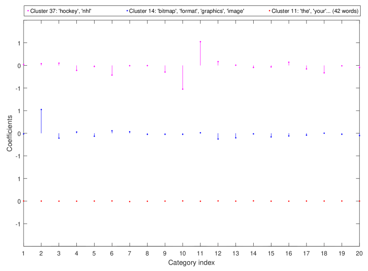
Figure 2: Newsgroup data: the coefficients of some word clusters obtained by CRL in response to the 20 categories.

Next, we study the interpretability of the CRL model. Figure 2 plots the coefficients for three clusters for illustration purposes. Note that we did not use any available word groups from the literature, which may or may not be useful for modeling the responses here.

First, cluster 14, composed of words bitmap, format, graphics, and image, shows a single large coefficient in response to category 2. This is sensible, as the documentation shows that the category corresponds to computer graphics.

Cluster 37 contains two words only, hockey and nhl. This group has two big coefficients in magnitude, $+2.25$ and $-1.05$ for the categories of hockey and baseball, respectively. So the occurrence of these two words seems helpful for differentiating the two related sport categories.

Finally, let’s turn to cluster 11 which consists of 42 words. All its coefficients are pretty small, varying between $-0.02$ and $0.01$ for different responses. A careful examination of its composition explains the mild effects: almost all are the so-called ‘stop words’, such as the, very, and yours, and removing this cluster gave almost identical results. CRL was able to capture these essentially irrelevant features and group them together. To sum up, CRL contributes as a beneficial complement to conventional variable selection.

6 Conclusions

Many high-dimensional methods adopt the “bet on sparsity” principle (Hastie et al.,, 2009), but in real multi-response applications, statisticians often face “dense” problems with such a large number of relevant features that variable selection may be ineffective. This paper proposed a clustered reduced-rank learning framework to build a predictive and interpretable model through feature auto-grouping and dimension reduction.

The joint matrix regularization formulation poses intriguing challenges in both theory and computation. We provided universal information-theoretical limits to reveal the intrinsic cost of seeking for clusters, as well as the benefit of accumulating a large number of response variables in multivariate learning. The obtained error rates are strikingly different from those assuming sparsity. Moreover, we proved that CRL, unlike the class of methods based on pairwise-difference penalization, achieves the minimax optimal rate in some common scenarios. The remarkable fact that the CRL estimators need not be global minimizers but just fixed points in some regular problems paved the way for the design of an efficient optimization algorithm in the nonconvex setup. Furthermore, a new information criterion, along with its scale-free form, was proposed to address cluster and rank selection. Overall, our new method is as interpretable as variable selection, and is advantageous when the numbers of relevant features and irrelevant features are of the same order, or when the number of responses is greater than the number of features up to a multiplicative constant.

CRL can be extended to tensors, and one possible application is model segmentation in a multi-task setting. For example, given $\boldsymbol{Y}=[\tilde{\boldsymbol{y}}_{1},\ldots\tilde{\boldsymbol{y}}_{n}]^{T}$, $\boldsymbol{X}=[\tilde{\boldsymbol{x}}_{1},\ldots\tilde{\boldsymbol{x}}_{n}]^{T}$ and an unknown order-3 tensor $\boldsymbol{B}\in\mathbb{R}^{p\times m\times n}$, we can fit a model $\tilde{\boldsymbol{y}}_{i}^{T}\sim\tilde{\boldsymbol{x}}_{i}^{T}\boldsymbol{B}_{::i}$ ($1\leq i\leq n$) by enforcing low rank in $\boldsymbol{B}$ and equisparsity along its third dimension. This can be applied to heterogeneous populations. Moreover, our algorithm often shows a linear convergence rate for small $q$ and $r$, which deserves further study. Finally, to reduce the search cost (thereby the overall error rate), one possible way is to limit the min/max cluster size; a new form of regularization (convex or nonconvex) that guarantees both interpretability and efficiency is an interesting topic that merits future research.

Appendix A Technical Details

Throughout the proofs, we use $C$, $c$, $L$ to denote positive constants unless otherwise mentioned. They are not necessarily the same at each occurrence. Given any matrix $\boldsymbol{A}$, we use $cs(\boldsymbol{A})$ and $rs(\boldsymbol{A})$ to denote its column space and row space, respectively. Denote by ${{\mathcal{P}}}_{\boldsymbol{A}}$ the orthogonal projection matrix onto $cs(\boldsymbol{A})$, i.e., ${{\mathcal{P}}}_{\boldsymbol{A}}=\boldsymbol{A}(\boldsymbol{A}^{T}\boldsymbol{A})^{+}\boldsymbol{A}^{T}$, and by ${{\mathcal{P}}}_{\boldsymbol{A}}^{\perp}$ the projection onto its orthogonal complement. We use $\boldsymbol{A}[\mathcal{I},\mathcal{J}]$ to denote a submatrix of $\boldsymbol{A}$ with rows and columns indexed by $\mathcal{I}$ and $\mathcal{J}$, respectively. The standard vectorization operator is denoted by $\operatorname{\mbox{vec}\,}(\cdot)$. Let $\mathbb{Z}$ be the set of integers and $[p]$ be $\{1,\ldots,p\}$. Given $x\in\mathbb{R}$, $\lfloor x\rfloor$ and $\lceil x\rceil$ denote the floor and ceiling functions, respectively. Throughout the whole section, we abbreviate $\|\boldsymbol{B}\|_{2,\mathcal{C}}$ as $q(\boldsymbol{B})$, and $\mathrm{rank}(\boldsymbol{B})$ as $r(\boldsymbol{B})$.

Beyond the regression model, the canonical generalized linear models (GLMs) are widely used in statistics modeling. Here, $\boldsymbol{Y}\in\mathcal{Y}^{n\times m}\subset\mathbb{R}^{n\times m}$ has density $P_{\boldsymbol{\eta}}(\cdot)=\exp\{(\langle\cdot,\boldsymbol{\eta}\rangle-{b}(\boldsymbol{\eta}))/\sigma^{2}-c(\cdot,\sigma^{2})\}\$ with respect to measure $\nu_{0}$ defined on $\mathcal{Y}^{n\times m}$ (typically the counting measure or Lebesgue measure), where $\boldsymbol{\eta}\in\mathbb{R}^{n\times m}$ represents the systematic component of interest, and $\sigma$ is the scale parameter; see Jørgensen, (1987). Since $\sigma$ is not the parameter of interest, it is more convenient to define the density $\exp\{(\langle\cdot,\boldsymbol{\eta}\rangle-{b}(\boldsymbol{\eta}))/\sigma^{2}\}$ (still written as $P_{\boldsymbol{\eta}}(\cdot)$ with a slight abuse of notation) with respect to the base measure $\,\mathrm{d}\nu=\exp(-c(\cdot,\sigma^{2}))\,\mathrm{d}\nu_{0}$. The scaled loss for $\boldsymbol{\eta}$ can be written as

$$l_{0}(\boldsymbol{\eta};\boldsymbol{Y})=\{-\langle\boldsymbol{Y},\boldsymbol{\eta}\rangle+b(\boldsymbol{\eta})\}/\sigma^{2}.$$ (A.1)

That is, $l_{0}$ corresponds to a distribution in the exponential dispersion family with cumulant function $b(\cdot)$, dispersion $\sigma^{2}$ and natural parameter $\boldsymbol{\eta}$. In the Gaussian case, $b(\cdot)=\|\cdot\|_{F}^{2}/2$. Define the natural parameter space (assumed to be nonempty)

$$\Omega=\{\boldsymbol{\eta}\in\mathbb{R}^{n\times m}:b(\boldsymbol{\eta})<\infty\}.$$ (A.2)

When $\Omega$ is open, $p_{\boldsymbol{\eta}}$ is called regular, and $b$ can be shown to be differentiable to any order and convex, as is well known in the statistics literature (see, e.g., Wainwright and Jordan, (2008)).

A.1 Minimax lower bounds

We prove a more general theorem including the lower bounds for both the estimation error and the prediction error.

Theorem A.1.

Assume $\boldsymbol{Y}|\boldsymbol{X}\boldsymbol{B}^{*}$ follows a distribution in the regular exponential family with dispersion $\sigma^{2}$ with $l_{0}$ the associated negative log-likelihood function defined in (A.1), and define a signal class by

$$\boldsymbol{B}^{*}\in\mathcal{S}(q,r)=\{\boldsymbol{B}\in\mathbb{R}^{p\times m}:q(\boldsymbol{B})\leq q,r(\boldsymbol{B})\leq r\},$$

where $p\geq q\geq r\geq 2$, $r(q\wedge r(\boldsymbol{X})+m-r)\geq 4$. Let $b,\zeta$ be any integers satisfying $\sum_{i=0}^{\zeta}{r\choose i}(b-1)^{i}\geq q$, with $b\geq 2,1\leq\zeta\leq r$, and define a complexity function

$$P(q,r)=(q+m)r+p\{\log(er)-\log\log q\}.$$ (A.3)

(a) Assume that ${\mathbf{\Delta}}_{l_{0}}(\boldsymbol{0},\boldsymbol{X}\boldsymbol{B})\sigma^{2}\leq\kappa{\mathbf{D}}_{2}(\boldsymbol{0},\boldsymbol{B})$ for any $\boldsymbol{B}\in\mathcal{S}(q,r)$. Then there exist positive constants $c,c^{\prime}$, depending on $I(\cdot)$ only, such that

$$\inf_{\hat{\boldsymbol{B}}}\sup_{\boldsymbol{B}^{*}\in\mathcal{S}(q,r)}\,\mathbb{E}\left\{I\Big{(}\|\boldsymbol{B}^{*}-\hat{\boldsymbol{B}}\|_{F}^{2}{\big{/}}\Big{[}c\sigma^{2}\big{\{}(q+m)r+\frac{p\log q}{b^{2}\zeta}\big{\}}/\kappa\Big{]}\Big{)}\right\}\geq c^{\prime}>0,$$ (A.4)

In particular, under $8\leq q\leq\exp(r)$,

$$\inf_{\hat{\boldsymbol{B}}}\,\sup_{\boldsymbol{B}^{*}\in\mathcal{S}(q,r)}\mathbb{E}\big{[}I\big{(}\|\boldsymbol{B}^{*}-\hat{\boldsymbol{B}}\|_{F}^{2}/\{c\sigma^{2}P(q,r)/\kappa\}\big{)}\big{]}\geq c^{\prime}>0.$$ (A.5)

(b) Let the SVD of $\boldsymbol{X}$ be $\boldsymbol{U}\boldsymbol{D}\boldsymbol{V}^{T}$ and define $\boldsymbol{Z}=\boldsymbol{U}\boldsymbol{D}\in\mathbb{R}^{n\times r(\boldsymbol{X})}$. Assume the following restricted condition-number condition: when $q\leq r(\boldsymbol{X})$, there exist $\underline{\kappa},\overline{\kappa}$ such that $\underline{\kappa}{\mathbf{D}}_{2}(\boldsymbol{B}_{1},\boldsymbol{B}_{2})\leq{\mathbf{D}}_{2}(\boldsymbol{X}\boldsymbol{B}_{1},\boldsymbol{X}\boldsymbol{B}_{2})$, ${\mathbf{\Delta}}_{l_{0}}(\boldsymbol{0},\boldsymbol{X}\boldsymbol{B}_{1})\sigma^{2}\leq\overline{\kappa}{\mathbf{D}}_{2}(\boldsymbol{0},\boldsymbol{B}_{1})$ for any $\boldsymbol{B}_{i}\in\mathcal{S}(q,r)$ and $\underline{\kappa}/\overline{\kappa}$ is a positive constant; when $q>r(\boldsymbol{X})$, $\underline{\kappa}{\mathbf{D}}_{2}(\boldsymbol{C}_{1},\boldsymbol{C}_{2})\leq{\mathbf{D}}_{2}(\boldsymbol{Z}\boldsymbol{C}_{1},\boldsymbol{Z}\boldsymbol{C}_{2})$, ${\mathbf{\Delta}}_{l_{0}}(\boldsymbol{0},\boldsymbol{Z}\boldsymbol{C}_{1})\sigma^{2}\leq\overline{\kappa}{\mathbf{D}}_{2}(\boldsymbol{0},\boldsymbol{C}_{1})$ for any $\boldsymbol{C}_{i}:r(\boldsymbol{C}_{i})\leq r$ and $\underline{\kappa}/\overline{\kappa}$ is a positive constant.

Then there exist constants $c,c^{\prime}>0$, depending on $I(\cdot)$ only, such that when $q\leq r(\boldsymbol{X})$

$$\inf_{\hat{\boldsymbol{B}}}\sup_{\boldsymbol{B}^{*}\in\mathcal{S}(q,r)}\,\mathbb{E}\left\{I\Big{(}\|\boldsymbol{X}\boldsymbol{B}^{*}-\boldsymbol{X}\hat{\boldsymbol{B}}\|_{F}^{2}{\big{/}}\Big{[}c\sigma^{2}\big{\{}(q+m)r+\frac{p\log q}{b^{2}\zeta}\big{\}}\Big{]}\Big{)}\right\}\geq c^{\prime}>0,$$ (A.6)

and when $q>r(\boldsymbol{X})$,

$$\inf_{\hat{\boldsymbol{B}}}\sup_{\boldsymbol{B}^{*}\in\mathcal{S}(q,r)}\,\mathbb{E}(I[\|\boldsymbol{X}\boldsymbol{B}^{*}-\boldsymbol{X}\hat{\boldsymbol{B}}\|_{F}^{2}/\{c\sigma^{2}(r(\boldsymbol{X})+m)r\}])\geq c^{\prime}>0.$$ (A.7)

In particular, when $8\leq q\leq\exp(r)$ and $q\leq r(\boldsymbol{X})$,

$$\inf_{\hat{\boldsymbol{B}}}\sup_{\boldsymbol{B}^{*}\in{\mathcal{S}}(q,r)}\allowbreak\,\mathbb{E}\big{[}\|\boldsymbol{X}\boldsymbol{B}^{*}-\boldsymbol{X}\hat{\boldsymbol{B}}\|_{F}^{2}\big{]}\geq c\sigma^{2}P(q,r).$$

Proof.

We first introduce some standard notations and symbols in coding theory. Let $V_{q}(n,d)$ denote the volume of a Hamming ball of radius $d\leq q$ in $\{0,1,\ldots,q-1\}$, i.e.,

$$V_{q}(n,d)=\sum_{i=0}^{\lfloor d\rfloor}{n\choose i}(q-1)^{i}.$$

Given $q\geq 2$, $x\in[0,1]$, define the $q$-ary entropy function

$$h_{q}(x)=x\log_{q}(q-1)-x\log_{q}x-(1-x)\log_{q}(1-x),$$

and $h_{2}(x)$ is the Shannon entropy function. It is easy to see some basic facts: $h_{q}(x)\log q\allowbreak+\mbox{KL}(x\|\frac{q-1}{q})=\log q$, $h_{q}(0)=0$, $h_{q}(1-1/q)=1$ and $h_{q}(\cdot)$ is continuous and increasing in $[0,1-1/q]$. Here, the Kullback-Leibler divergence $\mbox{KL}(x\|y)=x\log(x/y)+(1-x)\log((1-x)/(1-y))$ for $x,y\in[0,1]$.

The following result is well known; see, e.g., van Lint, (1982).

Lemma A.1.

Let $q\geq 2$, $d\in[0,n(1-1/q)]$, and $q,d\in\mathbb{Z}$. Then

$$V_{q}(n,d)\leq q^{h_{q}(\theta)n},\ V_{q}(n,d)\geq{n\choose d}(q-1)^{d}\geq q^{h_{q}(\theta)n}\exp(-c\log n-c^{\prime}),$$

where $\theta=d/n$, and $c,c^{\prime}$ are positive constants.

The next lemma is essentially the Gilbert-Varshamov bound for $q$-ary codes, adapted for our purposes.

Lemma A.2.

Let $\Omega=\{\boldsymbol{a}=[a_{1},\ldots,a_{n}]^{T}:a_{j}\in\mathcal{A}\}$, where $|\mathcal{A}|=q$, $n\geq q>1$. Then there exists a subset $\{\boldsymbol{a}^{0},\ldots,\boldsymbol{a}^{M}\}\subset\Omega$ such that $\boldsymbol{a}^{0}\in\mathcal{A}^{n}$ is arbitrarily chosen, and

$$\log M\geq\log(q^{n}/V_{q}(n,\lceil d\rceil-1)-1)\geq c_{1}n\log q,$$ (A.8)

$$\rho(\boldsymbol{a}^{j},\boldsymbol{a}^{k})\geq c_{2}n,\ \forall 0\leq j<k\leq M,$$ (A.9)

where $\rho(\boldsymbol{a},\boldsymbol{a}^{\prime})=\sum_{i=1}^{n}1_{a_{j}\neq a_{j}^{\prime}}$ and $c_{1},c_{2}$ are universal positive constants.

Proof.

We can use the ‘greedy algorithm’ (Tsybakov,, 2008; Pellikaan et al.,, 2017) and Lemma A.1 to prove the result. Some details are as follows.

Let $d=c_{2}n$. Given any $\boldsymbol{a}\in\Omega$, the number of elements in $\{\boldsymbol{b}\in\Omega$: $\rho(\boldsymbol{b},\boldsymbol{a})\leq l\}=:B_{q}(\boldsymbol{a};l)$ is no more than $\sum_{i=0}^{l}{n\choose i}(q-1)^{i}$ or $V_{q}(n,l).$

Consider the following procedure to partition $\Omega$. Let $\boldsymbol{a}^{0}\in\mathcal{A}^{n}$ be arbitrarily chosen and $\Omega^{0}=\Omega$. Given $\boldsymbol{a}^{t}\in\Omega^{t}$ ($t\geq 0$), construct $L^{t}=\{\boldsymbol{a}\in B_{q}(\boldsymbol{a}^{t};\lceil d\rceil-1)\}\cap\Omega^{t}$ and $\Omega^{t+1}=\Omega^{t}\setminus L^{t}$, and choose an arbitrary $\boldsymbol{a}^{t+1}\in\Omega^{t+1}$. Repeat the process until $\Omega^{M+1}=\emptyset$. Then $L^{t}$ $(0\leq t\leq M)$ form a partition of $\Omega$, and so

$$(M+1)V_{q}(n,\lceil d\rceil-1)\geq q^{n}.$$

By Lemma A.1, for $d/n\leq 1-1/q$, or $c_{2}\leq 1-1/q$,

$${M+1}\geq q^{(1-h_{q}(c_{2}))n}.$$

It is not difficult to show that with a small enough $c_{2}$, $q^{(1-h_{q}(c_{2}))n}\geq 1+q^{c_{1}n}$ holds for all $n\geq q\geq 2$ and some constant $c_{1}>0$. The conclusion follows. ∎

Lemma A.3.

For $P_{\boldsymbol{X}\boldsymbol{B}}$ in the regular exponential family, the Kullback-Leibler divergence of $P_{\boldsymbol{X}\boldsymbol{B}_{2}}$ from $P_{\boldsymbol{X}\boldsymbol{B}_{1}}$ satisfies

$$\mbox{KL}(P_{\boldsymbol{X}\boldsymbol{B}_{1}}\|P_{\boldsymbol{X}\boldsymbol{B}_{2}})={\mathbf{\Delta}}_{l_{0}}(\boldsymbol{X}\boldsymbol{B}_{2},\boldsymbol{X}\boldsymbol{B}_{1}),$$

where ${\mathbf{\Delta}}_{l_{0}}(\cdot,\cdot)$ is the generalized Bregman function defined in (8).

See Lemma 3(iii) of She et al., (2021).

We prove (b). The proof for (a) is similar and simpler. Consider three cases.

Case (i): $(p\log q)/(\zeta b^{2})\geq(q+m)r$ and $q\leq r(\boldsymbol{X})$. Recall that $b,\zeta$ are integers satisfying

$$V_{b}(r,\zeta)=\sum_{i=0}^{\zeta}{r\choose i}(b-1)^{i}\geq q,\ b\geq 2,1\leq\zeta\leq r.$$ (A.10)

Hence we can pick $q$ $r$-dimensional vectors to form a set $\mathcal{C}$ satisfying

$$\mathcal{|}\mathcal{C}|=q,\ \boldsymbol{0}\in\mathcal{C},\ C\subset\{\boldsymbol{c}\in\mathbb{R}^{r}:\|\boldsymbol{c}\|_{0}\leq\zeta,c_{k}\in\{0,1,\ldots,b-1\},1\leq k\leq r\}.$$

Next, construct

$${\mathcal{B}}^{1}(q,r)=\{\boldsymbol{B} =[\boldsymbol{b}_{1},\ldots,\boldsymbol{b}_{j},\ldots,\boldsymbol{b}_{p}]^{T}:\boldsymbol{b}_{j}[1:r]/(\gamma R)\in\mathcal{C}\mbox{ and }\boldsymbol{b}_{j}[(r+1):m]=\boldsymbol{0}\},$$

where $\gamma>0$ is a small constant to be chosen later, and

$$R=\sigma(\log q)^{1/2}/(\zeta b^{2}\overline{\kappa})^{1/2}.$$

Clearly, ${\mathcal{B}}^{1}(q,r)\subset\mathcal{S}(q,r)$, $r(\boldsymbol{B}_{1}-\boldsymbol{B}_{2})\leq r$ and $q(\boldsymbol{B}_{1}-\boldsymbol{B}_{2})\leq q^{2}\wedge V_{2b-1}(r,2\zeta)=q^{2}$ for any $\boldsymbol{B}_{i}\in{\mathcal{B}}^{1}(q,r)$.

Define a vector version of Hamming distance by

$$\rho(\boldsymbol{B}_{1},\boldsymbol{B}_{2})=\sum_{j=1}^{p}1_{\boldsymbol{B}_{1}[j,:]\neq\boldsymbol{B}_{2}[j,:]}.$$

From Lemma A.2, there exists a subset ${\mathcal{B}}^{10}(q,r)\subset{\mathcal{B}}^{1}(q,r)$ such that $\boldsymbol{0}\in{\mathcal{B}}^{10}(q,r)$ and

$$\log(|{\mathcal{B}}^{10}(q,r)|-1)\geq\log(q^{p}/(V_{q}(p,\lceil d\rceil-1)-1))\geq c_{1}p\log q,$$

$$\rho(\boldsymbol{B}_{1},\boldsymbol{B}_{2})\geq c_{2}p,\forall\boldsymbol{B}_{1},\boldsymbol{B}_{2}\in\mathcal{B}^{10},\boldsymbol{B}_{1}\neq\boldsymbol{B}_{2}$$

for some universal constants $c_{1},c_{2}>0$. Hence

$$\|\boldsymbol{B}_{1}-\boldsymbol{B}_{2}\|_{F}^{2}\geq\rho(\boldsymbol{B}_{1},\boldsymbol{B}_{2})\cdot 1\cdot\gamma^{2}R^{2}\geq c_{2}\gamma^{2}R^{2}p,\ \forall\boldsymbol{B}_{1},\boldsymbol{B}_{2}\in\mathcal{B}^{10}.$$

From the restricted conditional number assumption,

$$\|\boldsymbol{X}\boldsymbol{B}_{1}-\boldsymbol{X}\boldsymbol{B}_{2}\|_{F}^{2}\geq c_{2}\underline{\kappa}\gamma^{2}R^{2}p=\frac{c_{2}\underline{\kappa}}{\overline{\kappa}}\frac{p\log q}{\zeta b^{2}}\sigma^{2}\gamma^{2}$$ (A.11)

for any $\boldsymbol{B}_{1},\boldsymbol{B}_{2}\in\mathcal{B}^{10}$, $\boldsymbol{B}_{1}\neq\boldsymbol{B}_{2}$, where $c_{2}$, $\underline{\kappa}/\overline{\kappa}$ are positive constants.

From Lemma A.3 and the regularity condition, for any $\boldsymbol{B}\in{\mathcal{B}}^{10}(q,r)$, we have

$$\mbox{KL}(P_{\boldsymbol{X}\boldsymbol{B}}\|P_{\boldsymbol{0}})\leq\frac{\overline{\kappa}}{\sigma^{2}}{\mathbf{D}}_{2}(\boldsymbol{0},\boldsymbol{B})\leq\frac{1}{2\sigma^{2}}\overline{\kappa}(b-1)^{2}\gamma^{2}R^{2}\rho(\boldsymbol{0},\boldsymbol{B})\zeta\leq\frac{\zeta b^{2}\gamma^{2}}{2\sigma^{2}}\overline{\kappa}R^{2}p.$$

Therefore,

$$\frac{1}{|\mathcal{B}^{10}|-1}\sum_{\boldsymbol{B}\in\mathcal{B}^{10}\setminus\{\boldsymbol{0}\}}\mbox{KL}(P_{\boldsymbol{X}\boldsymbol{B}}\|P_{\boldsymbol{0}})\leq\gamma^{2}p\log q.$$ (A.12)

Combining (A.11) and (A.12) and choosing a sufficiently small value for $\gamma$, we can apply Theorem 2.7 of Tsybakov, (2008) to get the desired lower bound $(p\log q)/(\zeta b^{2})$.

Case (ii): $(q+m)r\geq(p\log q)/(\zeta b^{2})$ and $r(\boldsymbol{X})\geq q$. Consider a signal subclass

$${\mathcal{B}}^{2}(q,r)=\{\boldsymbol{B}=[b_{jk}]: \ b_{jk}=0\mbox{ or }\gamma R\mbox{ if }1\leq j\leq q-1,1\leq k\leq r/2$$

$$\mbox{ or }1\leq j\leq r/2,1\leq k\leq m,\mbox{ and }b_{jk}=0\mbox{ otherwise}\},$$

where $R={\sigma}/{{\overline{\kappa}^{1/2}}}$ and $\gamma>0$ is a small constant to be chosen later. Clearly, $|{\mathcal{B}}^{2}(q,r)|=2^{(q-1+m-r/2)r/2}\geq 2^{c(q+m)r}$, $\mathcal{B}^{2}(q,r)\subset\mathcal{S}(q,r)$, and $r(\boldsymbol{B}_{1}-\boldsymbol{B}_{2})\leq r$, $q(\boldsymbol{B}_{1}-\boldsymbol{B}_{2})\leq q,$ $\forall\boldsymbol{B}_{1},\boldsymbol{B}_{2}\in\mathcal{B}^{2}(q,r)$. In this case, we define the elementwise Hamming distance by

$$\rho(\boldsymbol{B}_{1},\boldsymbol{B}_{2})=\|\operatorname{\mbox{vec}\,}(\boldsymbol{B}_{1})-\operatorname{\mbox{vec}\,}(\boldsymbol{B}_{2})\|_{0}.$$

By Lemma A.2 and $(q-1+m-r/2)r/2\geq 2$, there exists a subset ${\mathcal{B}}^{20}(q,r)\subset{\mathcal{B}}^{2}(q,r)$ such that $\boldsymbol{0}\in{\mathcal{B}}^{20},$

$$\log(|{\mathcal{B}}^{20}(q,r)|-1)\geq c_{1}r(q+m),$$

and

$$\rho(\boldsymbol{B}_{1},\boldsymbol{B}_{2})\geq c_{2}r(q+m),\forall\boldsymbol{B}_{1},\boldsymbol{B}_{2}\in\mathcal{B}^{20},\boldsymbol{B}_{1}\neq\boldsymbol{B}_{2}$$

for some universal constants $c_{1},c_{2}>0$. Then for any $\boldsymbol{B}_{1},\boldsymbol{B}_{2}\in\mathcal{B}^{20}$

$$\|\boldsymbol{X}\boldsymbol{B}_{1}-\boldsymbol{X}\boldsymbol{B}_{2}\|_{F}^{2}\geq\underline{\kappa}\gamma^{2}R^{2}\rho(\boldsymbol{B}_{1},\boldsymbol{B}_{2})\geq c_{2}(\underline{\kappa}/\overline{\kappa})\sigma^{2}\gamma^{2}(q+m)r.$$

Furthermore, for any $\boldsymbol{B}\in\mathcal{B}^{20}(q,r)$, we have

$$\mbox{KL}(P_{\boldsymbol{X}\boldsymbol{B}}\|P_{\boldsymbol{0}})\leq\frac{1}{2\sigma^{2}}\overline{\kappa}\gamma^{2}R^{2}\rho(\boldsymbol{0},\boldsymbol{B})\leq{\gamma^{2}}(q+m)r.$$

The afterward treatment follows same lines as in (i) and the details are omitted.

Case (iii): $(r(\boldsymbol{X})\wedge q+m)r\geq(p\log q)/(\zeta b^{2})$ and $r(\boldsymbol{X})<q$. In this case, we have a more relaxed regularity condition that is imposed on the matrix $\boldsymbol{Z}$ with full column rank (and so it can hold even when $p>n$). Define $\tilde{\mathcal{S}}(r)=\{\boldsymbol{C}\in\mathbb{R}^{r(\boldsymbol{X})\times m}:r(\boldsymbol{C})\leq r\}$. Then for any estimator $\hat{\boldsymbol{B}}$, and $\hat{\boldsymbol{C}}=\boldsymbol{V}^{T}\hat{\boldsymbol{B}}$, we have

$$\sup_{\boldsymbol{B}^{*}\in\mathcal{S}(q,r)}\,\mathbb{P}\big{[}\|\boldsymbol{X}\boldsymbol{B}^{*}-\boldsymbol{X}\hat{\boldsymbol{B}}\|_{F}^{2}\geq c\sigma^{2}\{r(\boldsymbol{X})\wedge q+m\}r\big{]}$$

$$\geq\ \ \sup_{\boldsymbol{C}\in\tilde{\mathcal{S}}(r)}\,\mathbb{P}\big{[}\|\boldsymbol{Z}\boldsymbol{C}-\boldsymbol{Z}\hat{\boldsymbol{C}}\|_{F}^{2}\geq c\sigma^{2}\{r(\boldsymbol{X})\wedge q+m\}r\big{]},$$

because $\tilde{\mathcal{S}}(r)\subset\{\boldsymbol{V}^{T}\boldsymbol{B}^{*}:\boldsymbol{B}^{*}\in\mathcal{S}(q,r)\}$ under $r(\boldsymbol{X})<q$. Repeating the argument in case (ii) gives the result. (So for the purpose of prediction, using a $q$ greater than $r(\boldsymbol{X})$ is unnecessary.)

To show the specific rate (A.3) under $8\leq q\leq\exp(r)$, we need to pick proper $b,\zeta$ satisfying (A.10). Due to

$$V_{b}(r,\zeta)\geq{r\choose\zeta}(b-1)^{\zeta}\geq\Big{\{}\frac{(b-1)r}{\zeta}\Big{\}}^{\zeta},$$

our goal is to minimize $b^{2}\zeta$ subject to the constraint $(r(b-1)/\zeta)^{\zeta}\geq q$ or

$$b\geq q^{1/\zeta}\zeta/r+1.$$ (A.13)

Introduce

$$\phi=q^{1/r}>1,$$

and reparametrize $\zeta$ by

$$z=q^{1/\zeta}\in[\phi,q].$$

Because $\zeta=(\log q)/(\log z$) and (A.13) means $b\geq(z\log q)/(r\log z)+1(\geq 2)$, $b^{2}\zeta$ is greater than or equal to

$$f(z)=\Big{(}\frac{z}{r}\frac{\log q}{\log z}+1\Big{)}^{2}\,\frac{\log q}{\log z}.$$

Simple calculation shows

$$f^{\prime}(z)={g(z)(z\log q+r\log z)(\log q)^{2}}/\{zr^{2}(\log z)^{3}\}$$

where

$$g(z)=2z-3\frac{z}{\log z}-\frac{1}{\log\phi}.$$

It is easy to verify that $g(\cdot)$ is strictly increasing in its domain $[\phi,q]\subset(1,q]$. Since $\phi\leq e\leq 4.95$,

$$g(\phi)=(2\phi\log\phi-3\phi-1)/\log\phi<0.$$

Moreover, from as $q\geq 8>e^{2}$,

$$g(q)=(1/\log q)[q(2\log q-3)-r]>0.$$

Therefore, the minimum of $f$ is achieved at a point $z_{o}$ that satisfies $g(z_{o})=0$. But

$$g(5.3/\log\phi) \geq(5.3/\log\phi)(2-3/(\log(1/\log\phi)+5.3))-1/\log\phi$$

$$\geq(1/\log\phi)5.3(2-3/\log 5.3)-1/\log\phi\geq 0,$$

so $z_{o}\leq 5.3r/\log q$. Therefore,

$$f(z_{o})\leq f(5.3r/\log q)\leq\frac{c\log q}{\log(5.3r)-\log\log q},$$

and the corresponding $\frac{p\log q}{\zeta b^{2}}\geq cp(\log(er)\allowbreak-\log\log q)$ for some constant $c>0$. ∎

Remark 7.

The above scheme can yield other useful bounds in different situations. For example, simple calculation shows $f(\phi)=(q^{1/r}+1)^{2}r$, $f(q)=(q/r+1)^{2}$. Therefore, we also know that under $q\leq r(\boldsymbol{X})$, the minimax rate for the prediction error is greater than or equal to $\sigma^{2}\big{[}(q+m)r+\{(q^{1/r}+1)^{-2}r^{-1}\vee(q/r+1)^{-2}\}p\log q\big{]}.$ So when $\phi$ (or $q^{1/r}$) is sufficiently large, say, $\phi\geq 5$ or $q\geq 5^{r}$, the optimal $z_{o}$ takes $\phi$, and so the minimax error rate is no lower than $\sigma^{2}\{pq^{-2/r}r^{-1}\log q+(q+m)r\}$.

A.2 CRL’s upper error bounds

Given any $\boldsymbol{A}\in\mathbb{R}^{p\times m}$ satisfying $q(\boldsymbol{A})\leq q$, using the symbols introduced in Section 4.1, we can write $\boldsymbol{A}=\boldsymbol{F}{\boldsymbol{\mu}}$ with $\boldsymbol{F}\in\mathbb{R}^{p\times q}$, ${\boldsymbol{\mu}}\in\mathbb{R}^{q\times m}$. The binary membership matrix $\boldsymbol{F}$ fully characterizes the row clusters of $\boldsymbol{A}$. We give it a new notation $\mathcal{Q}(\boldsymbol{A})$, and abbreviate $\boldsymbol{X}{{\mathcal{P}}}_{\mathcal{Q}(\boldsymbol{A})}=\boldsymbol{X}\boldsymbol{F}(\boldsymbol{F}^{T}\boldsymbol{F})^{+}\boldsymbol{F}^{T}$ as $\boldsymbol{X}_{\mathcal{Q}(\boldsymbol{A})}$. Obviously, ${{\mathcal{P}}}_{\mathcal{Q}(\boldsymbol{A})}\boldsymbol{A}=\boldsymbol{A}$. Note that ${{\mathcal{P}}}_{\mathcal{Q}(\boldsymbol{A})}$ is permutation invariant: ${{\mathcal{P}}}_{\mathcal{Q}(\boldsymbol{A})\boldsymbol{P}}={{\mathcal{P}}}_{\mathcal{Q}(\boldsymbol{A})}$ for any permutation matrix $\boldsymbol{P}\in\mathbb{R}^{q\times q}$, namely, the row clusters are unlabeled in nature. Let $\hat{r}=r(\hat{\boldsymbol{B}})$, $\hat{q}=q(\hat{\boldsymbol{B}})$, $r^{*}=r(\boldsymbol{B}^{*})$, $q^{*}=q(\boldsymbol{B}^{*})$.

First, we prove Theorem 2. Using the $\iota$ notations in Section 4, we write

$$G_{\rho}(\boldsymbol{B};\boldsymbol{B}^{-})=l_{0}(\boldsymbol{X}\boldsymbol{B})-{\mathbf{\Delta}}_{l_{0}}(\boldsymbol{X}\boldsymbol{B},\boldsymbol{X}\boldsymbol{B}^{-})+\rho{\mathbf{D}}_{2}(\boldsymbol{B},\boldsymbol{B}^{-})+\iota(\boldsymbol{S})+\iota_{\boldsymbol{V}}(\boldsymbol{V}).$$

It follows from $G_{\rho}(\hat{\boldsymbol{B}};\hat{\boldsymbol{B}})\leq G_{\rho}(\boldsymbol{B}^{*};\hat{\boldsymbol{B}})$ that

$$l_{0}(\boldsymbol{X}\hat{\boldsymbol{B}})\leq l_{0}(\boldsymbol{X}\boldsymbol{B}^{*})-{\mathbf{\Delta}}_{l_{0}}(\boldsymbol{X}\boldsymbol{B}^{*},\boldsymbol{X}\hat{\boldsymbol{B}})+\rho{\mathbf{D}}_{2}(\boldsymbol{B}^{*},\hat{\boldsymbol{B}}),$$

or

$$2\bar{\mathbf{\Delta}}_{l_{0}}(\boldsymbol{X}\boldsymbol{B}^{*},\boldsymbol{X}\hat{\boldsymbol{B}})\leq\langle\boldsymbol{E},\boldsymbol{X}\hat{\boldsymbol{B}}-\boldsymbol{X}\boldsymbol{B}^{*}\rangle+\rho{\mathbf{D}}_{2}(\boldsymbol{B}^{*},\hat{\boldsymbol{B}}),$$ (A.14)

based on the definition of the generalized Bregman function (8).

To make our proof applicable to oracle inequalities, we study a more general stochastic term

$$\langle\boldsymbol{E},\boldsymbol{X}\boldsymbol{\Delta}\rangle$$

where $\boldsymbol{\Delta}=\hat{\boldsymbol{B}}-\boldsymbol{B}$ with $q(\boldsymbol{B})\leq q,r(\boldsymbol{B})\leq r$. Let $\hat{\mathcal{Q}}=\mathcal{Q}(\hat{\boldsymbol{B}})$, $\mathcal{Q}=\mathcal{Q}(\boldsymbol{B})$. Then $q(\boldsymbol{\Delta})\leq q^{2}$ and $r(\boldsymbol{\Delta})\leq 2r$. The stochastic term $\langle\boldsymbol{E},\boldsymbol{X}\boldsymbol{\Delta}\rangle$ must be treated carefully; otherwise $q^{2}$ will arise in the error bound. The following decomposition is key to our analysis:

$$\quad\ \langle\boldsymbol{E},\boldsymbol{X}\boldsymbol{\Delta}\rangle$$

$$=\langle\boldsymbol{E},\boldsymbol{X}\boldsymbol{\Delta}{{\mathcal{P}}}_{rs}+\boldsymbol{X}\boldsymbol{\Delta}{{\mathcal{P}}}_{rs}^{\perp}\rangle$$

$$=\langle\boldsymbol{E},\boldsymbol{X}\boldsymbol{\Delta}{{\mathcal{P}}}_{rs}+\boldsymbol{X}\hat{\boldsymbol{B}}{{\mathcal{P}}}_{rs}^{\perp}\rangle$$

$$=\langle\boldsymbol{E},{{\mathcal{P}}}_{\boldsymbol{X}_{\mathcal{Q}}}\boldsymbol{X}\boldsymbol{\Delta}{{\mathcal{P}}}_{rs}\rangle+\langle\boldsymbol{E},{{\mathcal{P}}}_{\boldsymbol{X}_{\mathcal{Q}}}^{\perp}\boldsymbol{X}\hat{\boldsymbol{B}}{{\mathcal{P}}}_{rs}\rangle+\langle\boldsymbol{E},\boldsymbol{X}\hat{\boldsymbol{B}}{{\mathcal{P}}}_{rs}^{\perp}\rangle$$

$$=\langle\boldsymbol{E},{{\mathcal{P}}}_{\boldsymbol{X}_{\mathcal{Q}}}\boldsymbol{X}\boldsymbol{\Delta}{{\mathcal{P}}}_{rs}\rangle+\langle\boldsymbol{E},{{\mathcal{P}}}_{\boldsymbol{X}_{\mathcal{Q}}}^{\perp}{{\mathcal{P}}}_{\boldsymbol{X}_{\hat{\mathcal{Q}}}}\boldsymbol{X}\hat{\boldsymbol{B}}{{\mathcal{P}}}_{rs}\rangle+\langle\boldsymbol{E},{{\mathcal{P}}}_{\boldsymbol{X}_{\hat{\mathcal{Q}}}}\boldsymbol{X}\hat{\boldsymbol{B}}{{\mathcal{P}}}_{rs}^{\perp}\rangle$$

$$=:\langle\boldsymbol{E},\boldsymbol{A}_{1}\rangle+\langle\boldsymbol{E},\boldsymbol{A}_{2}\rangle+\langle\boldsymbol{E},\boldsymbol{A}_{3}\rangle,$$

where ${{\mathcal{P}}}_{rs}$ is the orthogonal projection onto the row space of $\boldsymbol{X}\boldsymbol{B}$ and ${{\mathcal{P}}}_{rs}^{\perp}$ its orthogonal complement. Because of the orthogonality between $\boldsymbol{A}_{i}$,

$$\|\boldsymbol{A}_{1}\|_{F}^{2}+\|\boldsymbol{A}_{2}\|_{F}^{2}+\|\boldsymbol{A}_{3}\|_{F}^{2}=\|\boldsymbol{X}\boldsymbol{\Delta}\|_{F}^{2}.$$

It is easy to see that $r(\boldsymbol{A}_{1})\leq r({{\mathcal{P}}}_{rs})\leq r$, $r(\boldsymbol{A}_{2})\leq r(\hat{\boldsymbol{B}})\wedge r({{\mathcal{P}}}_{rs})\leq r$, $r(\boldsymbol{A}_{3})=r({{\mathcal{P}}}_{\boldsymbol{X}_{\hat{\mathcal{Q}}}}\boldsymbol{X}\hat{\boldsymbol{B}}{{\mathcal{P}}}_{rs}^{\perp})\leq\hat{r}\leq r$.

In the following, we use ${p\brace q}$ to denote the “Stirling number of the second kind”, i.e., the number of ways to partition a set of $p$ labeled objects into $q$ non-empty unlabeled subsets.

Lemma A.4.

Suppose that $\operatorname{\mbox{vec}\,}(\boldsymbol{E})$ is sub-Gaussian with mean zero and scale bounded by $\sigma$. Given $\boldsymbol{X}\in\mathbb{R}^{n\times p}$, $1\leq q\leq p$, $1\leq r\leq q$, define $\Gamma_{r,q}=\{\boldsymbol{A}:\boldsymbol{A}\in\mathbb{R}^{n\times m},\|\boldsymbol{A}\|_{F}\leq 1,r(\boldsymbol{A})\leq r,cs(\boldsymbol{A})\subset cs(\boldsymbol{X}_{\mathcal{Q}})\mbox{ for some }\mathcal{Q}:q(\mathcal{Q})\leq q\}$. Let

$$P(r,q)=(r(\boldsymbol{X})\wedge q+m)r+\log{p\brace q}.$$

Then for any $t\geq 0$,

$$\,\mathbb{P}[\sup_{\boldsymbol{A}\in\Gamma_{r,q}}\langle\boldsymbol{E},\boldsymbol{A}\rangle\geq t\sigma+\{L\sigma^{2}P(r,q)\}^{1/2}]\leq C\exp(-ct^{2}),$$ (A.15)

where $L,C,c>0$ are universal constants.

Lemma A.5.

Suppose $\operatorname{\mbox{vec}\,}(\boldsymbol{E})$ is sub-Gaussian with mean zero and scale bounded by $\sigma$. Given $\boldsymbol{X}\in\mathbb{R}^{n\times p}$, $1\leq q_{1},q_{2}\leq p$, $1\leq r\leq q_{2}$, define $\Gamma_{r,q_{1},q_{2}}=\{\boldsymbol{A}:\boldsymbol{A}\in\mathbb{R}^{n\times m},\|\boldsymbol{A}\|_{F}\leq 1,r(\boldsymbol{A})\leq r,cs(\boldsymbol{A})\subset cs({{\mathcal{P}}}_{\boldsymbol{X}_{\mathcal{Q}_{1}}^{\perp}}{{\mathcal{P}}}_{\boldsymbol{X}_{{\mathcal{Q}}_{2}}})\mbox{ with }q(\mathcal{Q}_{1})\allowbreak\leq q_{1},q(\mathcal{Q}_{2})\leq q_{2}\}$. Let

$$P(r,q_{1},q_{2})=(r(\boldsymbol{X})\wedge q_{2}+m)r+\log{p\brace q_{1}}+\log{p\brace q_{2}}.$$

Then for any $t\geq 0$,

$$\,\mathbb{P}[\sup_{\boldsymbol{A}\in\Gamma_{r,q_{1},q_{2}}}\langle\boldsymbol{E},\boldsymbol{A}\rangle\geq t\sigma+\{L\sigma^{2}P(r,q_{1},q_{2})\}^{1/2}]\leq C\exp(-ct^{2}),$$ (A.16)

where $L,C,c>0$ are universal constants.

Lemma A.6.

For any $p\geq 1$, $1\leq q\leq p$,

$$c_{1}(p-q)\log q\leq\log{p\brace q}\leq c_{2}(p-q)\log q,$$ (A.17)

where $c_{1},c_{2}$ are positive constants.

Let $P_{o}(q,r)=(r(\boldsymbol{X})\wedge q+m)r+(p-q)\log q$. For any $a,b,a^{\prime}>0$ and $4b>a$,

$$\langle\boldsymbol{E},\boldsymbol{A}_{1}\rangle-\|\boldsymbol{A}_{1}\|_{F}^{2}/a-bL\sigma^{2}P_{o}(q,r)$$

$$\leq \,\|\boldsymbol{A}_{1}\|_{F}\langle\boldsymbol{E},\boldsymbol{A}_{1}/\|\boldsymbol{A}_{1}\|_{F}\rangle-2({{b}/{a}})^{1/2}\|\boldsymbol{A}_{1}\|_{F}\{{L\sigma^{2}P_{o}(q,r)\}^{1/2}}$$

$$\leq \,\|\boldsymbol{A}_{1}\|_{F}^{2}/{a^{\prime}}+({a^{\prime}}/{4})R_{1}^{2},$$

where $L$ is a constant and

$$R_{1} :=\sup_{\boldsymbol{A}\in\Gamma_{r,q}}\big{[}\langle\boldsymbol{E},\boldsymbol{A}\rangle-2(b/a)^{1/2}\{{L\sigma^{2}P_{o}(q,r)\}^{1/2}}\big{]}_{+}.$$ (A.18)

We claim an expectation-form bound: $\,\mathbb{E}R_{1}^{2}\leq C\sigma^{2}$. In fact, from Lemmas A.4 and A.6,

$$\begin{split}&\,\mathbb{P}\big{[}\sup_{\boldsymbol{A}\in\Gamma_{r,q}}\langle\boldsymbol{E},\boldsymbol{A}\rangle-\{L\sigma^{2}P_{o}(q,r)\}^{1/2}\\ &\qquad\geq t\sigma+2(b/a)^{1/2}\sigma\{{LP_{o}(q,r)\}^{1/2}}-\sigma\{{LP_{o}(q,r)}\}^{1/2}\big{]}\\ \leq&C\exp(-ct^{2})\exp\Big{(}-c\big{[}\{2(b/a)^{1/2}-1\}^{2}LP_{o}(q,r)\big{]}\Big{)}\\ \leq&C\exp(-ct^{2}),\end{split}$$ (A.19)

and so $\,\mathbb{P}(R_{1}\geq t\sigma)\leq C\exp(-ct^{2})$.

Since $\hat{r}\leq r$, $\langle\boldsymbol{E},\boldsymbol{A}_{2}\rangle$ and $\langle\boldsymbol{E},\boldsymbol{A}_{3}\rangle$ can be similarly bounded using Lemma A.4 and Lemma A.5. To sum up,

$$\,\mathbb{E}\langle\boldsymbol{E},\boldsymbol{X}\boldsymbol{\Delta}\rangle\leq\,\mathbb{E}\left\{\Big{(}\frac{2}{a}+\frac{2}{a^{\prime}}\Big{)}\frac{\|\boldsymbol{X}\boldsymbol{\Delta}\|_{F}^{2}}{2}+4bL\sigma^{2}P_{o}(q,r)+Ca^{\prime}\sigma^{2}\right\}$$ (A.20)

for any $a,b,a^{\prime}>0$ and $4b>a$.

Substituting $\boldsymbol{B}^{*}$ for $\boldsymbol{B}$ in (A.20) and plugging it back to (A.14), we obtain

$$\,\mathbb{E}[2\bar{\mathbf{\Delta}}_{l_{0}}(\boldsymbol{X}\boldsymbol{B}^{*},\boldsymbol{X}\hat{\boldsymbol{B}})]$$

$$\leq\ \,\mathbb{E}\Big{\{}\big{(}\frac{2}{a}+\frac{2}{a^{\prime}}\big{)}{\mathbf{D}}_{2}(\boldsymbol{X}\hat{\boldsymbol{B}},\boldsymbol{X}\boldsymbol{B}^{*})+\rho{\mathbf{D}}_{2}(\boldsymbol{B}^{*},\hat{\boldsymbol{B}})\Big{\}}$$

$$+4bL\sigma^{2}[(r(\boldsymbol{X})\wedge q+m)r+(p-q)\log q]+Ca^{\prime}\sigma^{2}.$$

From the regularity condition,

$$\rho{\mathbf{D}}_{2}(\boldsymbol{B}^{*},\hat{\boldsymbol{B}})\leq(2\bar{\mathbf{\Delta}}_{l_{0}}-\delta{\mathbf{D}}_{2})(\boldsymbol{X}\boldsymbol{B}^{*},\boldsymbol{X}\hat{\boldsymbol{B}})+K\sigma^{2}\{(r(\boldsymbol{X})\wedge q+m)r+(p-q)\log q\},$$

and so

$$\,\mathbb{E}\Big{\{}\big{(}\delta-\frac{2}{a}-\frac{2}{a^{\prime}}\big{)}{\mathbf{D}}_{2}(\boldsymbol{X}\hat{\boldsymbol{B}},\boldsymbol{X}\boldsymbol{B}^{*})\Big{\}}\leq(4bL+K)\sigma^{2}\big{[}(r(\boldsymbol{X})\wedge q+m)r+(p-q)\log q\big{]}+Ca^{\prime}\sigma^{2}.$$

Choosing $a=a^{\prime}=8/\delta,b=3/\delta$ gives the conclusion.

To prove Theorem 3, we first notice that the optimality of $\hat{\boldsymbol{B}}$ and the definition of the effective noise imply

$${\mathbf{\Delta}}_{l_{0}}(\boldsymbol{X}\hat{\boldsymbol{B}},\boldsymbol{X}\boldsymbol{B}^{*})\leq\langle\boldsymbol{E},\boldsymbol{X}(\hat{\boldsymbol{B}}-\boldsymbol{B}^{*})\rangle,$$

in place of (A.14). Based on the stochastic term decomposition and the bounds in the lemmas, we have for any $a,a^{\prime},b>0$ and $4b>a$

$$\,\mathbb{E}\big{\{}{\mathbf{\Delta}}_{l_{0}}(\boldsymbol{X}\hat{\boldsymbol{B}},\boldsymbol{X}\boldsymbol{B}^{*})-(\frac{2}{a}+\frac{2}{a^{\prime}}){\mathbf{D}}_{2}(\boldsymbol{X}\hat{\boldsymbol{B}},\boldsymbol{X}\boldsymbol{B}^{*})\big{\}}$$

$$\leq\ 4bL\sigma^{2}\{(r(\boldsymbol{X})\wedge q+m)r+(p-q)\log q\}+Ca^{\prime}\sigma^{2}.$$

The conclusion can be shown similarly.

Next, we prove Corollary 1. By the optimality of $\hat{\boldsymbol{B}}$, we have $l_{0}(\boldsymbol{X}\hat{\boldsymbol{B}};\boldsymbol{Y})\leq l_{0}(\boldsymbol{X}\boldsymbol{B};\boldsymbol{Y})$ for any $\boldsymbol{B}:r(\boldsymbol{B})\leq r$, $q(\boldsymbol{B})\leq q$, from which it follows that

$${\mathbf{D}}_{l_{0}}(\boldsymbol{X}\hat{\boldsymbol{B}},\boldsymbol{X}\boldsymbol{B}^{*})\leq{\mathbf{D}}_{l_{0}}(\boldsymbol{X}\boldsymbol{B},\boldsymbol{X}\boldsymbol{B}^{*})+\langle\boldsymbol{E},\boldsymbol{X}\boldsymbol{\Delta}\rangle,$$

where $\boldsymbol{\Delta}=\hat{\boldsymbol{B}}-\boldsymbol{B}$. From (A.20) and the Cauchy-Schwartz inequality,

$$\,\mathbb{E}{\mathbf{D}}_{l_{0}}(\boldsymbol{X}\hat{\boldsymbol{B}},\boldsymbol{X}\boldsymbol{B}^{*})\leq\ \,\mathbb{E}\big{[}{\mathbf{D}}_{l_{0}}(\boldsymbol{X}\boldsymbol{B},\boldsymbol{X}\boldsymbol{B}^{*})+({2}/{a}+{2}/{a^{\prime}})(1+1/b^{\prime}){\mathbf{D}}_{2}(\boldsymbol{X}\hat{\boldsymbol{B}},\boldsymbol{X}\boldsymbol{B}^{*})$$

$$+({2}/{a}+{2}/{a^{\prime}})(1+b^{\prime}){\mathbf{D}}_{2}(\boldsymbol{X}\boldsymbol{B},\boldsymbol{X}\boldsymbol{B}^{*})\big{]}+4bL\sigma^{2}P_{o}(q,r)+Ca^{\prime}\sigma^{2},$$

for any $a,a^{\prime},b^{\prime}>0$ and $4b>a$. Choosing $a=a^{\prime}=16/\mu$, $b=5/\mu$, and $b^{\prime}=1$, and using the strongly convexity of $l_{0}$, we obtain the oracle inequality.

To prove the second result in the corollary, we set $\boldsymbol{B}=\boldsymbol{B}^{*}$ and use a high-probability form of (A.20): with probability at least $1-C\exp(-c(r(\boldsymbol{X})+m))$,

$$\langle\boldsymbol{E},\boldsymbol{X}\boldsymbol{\Delta}\rangle\leq\Big{(}\frac{2}{a}+\frac{2}{a^{\prime}}\Big{)}\frac{\|\boldsymbol{X}\boldsymbol{\Delta}\|_{F}^{2}}{2}+4bL\sigma^{2}P_{o}(q,r),$$ (A.21)

where as before, $L$ is a constant and $a,a^{\prime},b$ are any positive numbers satisfying $4b>a$. We use (A.19) to verify the probability bound under $2\leq q\leq p$: if $r=0$, $R_{1}=0$, otherwise

$$\{q\wedge r(\boldsymbol{X})\}r+(p-q)\log q\gtrsim r(\boldsymbol{X})\wedge\{q+(p-q)\log q\}\gtrsim r(\boldsymbol{X})\wedge p=r(\boldsymbol{X}).$$

(To see the last inequality, consider two cases $q\leq cp$ and $q\geq cp$.) Hence $(q\wedge r(\boldsymbol{X})+m)r+(p-q)\log q\gtrsim m+r(\boldsymbol{X})$.

Now, using $\log q\leq\vartheta+\log q^{*}\leq\vartheta\log q^{*}$, (A.21) implies

$$\Big{(}\mu-\frac{2}{a}-\frac{2}{a^{\prime}}\Big{)}\|\boldsymbol{X}\hat{\boldsymbol{B}}-\boldsymbol{X}\boldsymbol{B}^{*}\|_{F}^{2}\leq 8b\vartheta^{2}L\sigma^{2}\{(q^{*}\wedge r(\boldsymbol{X})+m)r^{*}+(p-q^{*})\log q^{*}\}$$

The remaining details are omitted.

Proofs of Lemma A.4 and Lemma A.5. We prove Lemma A.5 as follows. The proof of Lemma A.4 is similar. By definition, for any fixed $\boldsymbol{A}$, $\langle\boldsymbol{E},\boldsymbol{A}\rangle$ is a sub-Gaussian random variable with scale bounded by $\sigma\|\boldsymbol{A}\|_{F}$. Therefore, $\{\langle\boldsymbol{E},\boldsymbol{A}\rangle:\boldsymbol{A}\in\Gamma_{r,q_{1},q_{2}}\}$ defines a stochastic process with sub-Gaussian increments. The induced metric on $\Gamma_{r,q_{1},q_{2}}$ is Euclidean: $d(\boldsymbol{A}_{1},\boldsymbol{A}_{2})=\sigma\|\boldsymbol{A}_{1}-\boldsymbol{A}_{2}\|_{F}$.

We will use Dudley’s entropy integral to bound $\sup_{\boldsymbol{A}\in\Gamma_{r,q_{1},q_{2}}}\langle\boldsymbol{E},\boldsymbol{A}\rangle$. Toward this, we need to calculate the metric entropy $\log{\mathcal{N}}(\varepsilon,\Gamma_{r,q_{1},q_{2}},d)$, where ${\mathcal{N}}(\varepsilon,\Gamma_{r,q_{1},q_{2}},d)$ is the minimum cardinality of all $\varepsilon$-nets covering $\Gamma_{r,q_{1},q_{2}}$ under $d$.

Given $\boldsymbol{A}\in\Gamma_{r,q_{1},q_{2}}$, its column space must be contained in $cs({{\mathcal{P}}}_{\boldsymbol{X}_{\mathcal{Q}_{1}}^{\perp}}{{\mathcal{P}}}_{\boldsymbol{X}_{{\mathcal{Q}}_{2}}})$ for some $\mathcal{Q}_{i}$ with $q(\mathcal{Q}_{i})=q_{i}$. When varying $\mathcal{Q}_{i}$, the number of all $cs({{\mathcal{P}}}_{\boldsymbol{X}_{\mathcal{Q}_{1}}^{\perp}}{{\mathcal{P}}}_{\boldsymbol{X}_{{\mathcal{Q}}_{2}}})$ is no more than ${p\brace q_{1}}\times{p\brace q_{2}}$. Let $\mathcal{U}$ be a set of $\boldsymbol{U}_{i}$ with $\boldsymbol{U}_{i}\in\mathbb{R}^{n\times(r(\boldsymbol{X})\wedge q_{2})}$, $\boldsymbol{U}_{i}^{T}\boldsymbol{U}_{i}=\boldsymbol{I}$, and $\boldsymbol{U}_{i}\boldsymbol{U}_{i}^{T}$ characterizing all these column spaces, $1\leq i\leq{p\brace q_{1}}\times{p\brace q_{2}}$. Then we can represent $\boldsymbol{A}$ by

$$\boldsymbol{A}=\boldsymbol{U}\boldsymbol{\Sigma}\boldsymbol{V}^{T},$$ (A.22)

where $\boldsymbol{U}\in\mathcal{U}$, $\boldsymbol{V}\in\mathbb{O}^{m\times r}$, and $\boldsymbol{\Sigma}\in\mathbb{R}^{(r(\boldsymbol{X})\wedge q_{2})\times r}$.

An $\varepsilon$-net can be designed noticing that $\boldsymbol{V}\boldsymbol{V}^{T}$ corresponds to a point on a Grassmann manifold $G_{m,r}$ (all $r$-dimensional subspaces of $\mathbb{R}^{m}$), and $\boldsymbol{\Sigma}=\boldsymbol{U}^{T}\boldsymbol{A}\boldsymbol{V}$ is in a unit ball of dimensionality ${(r(\boldsymbol{X})\wedge q_{2})\times r}$, denoted by $B_{(r(\boldsymbol{X})\wedge q_{2})\times r}$. In fact, given any $\boldsymbol{A}_{1}\in\Gamma_{r,q_{1},q_{2}}$, we can write $\boldsymbol{A}_{1}=\boldsymbol{U}_{1}\boldsymbol{\Sigma}_{1}\boldsymbol{V}_{1}^{T}$ according to (A.22) and find $\boldsymbol{V}_{2}$ and $\boldsymbol{\Sigma}_{2}$ such that $\|\boldsymbol{V}_{1}\boldsymbol{V}_{1}^{T}-\boldsymbol{V}_{2}\boldsymbol{V}_{2}^{T}\|_{2}\leq\varepsilon$ and $\|\boldsymbol{\Sigma}_{1}\boldsymbol{V}_{1}^{T}\boldsymbol{V}_{2}-\boldsymbol{\Sigma}_{2}\|_{F}\leq\varepsilon$. Then, for $\boldsymbol{A}_{2}=\boldsymbol{U}_{1}\boldsymbol{\Sigma}_{2}\boldsymbol{V}_{2}^{T}$,

$$\|\boldsymbol{A}_{1}-\boldsymbol{A}_{2}\|_{F} \leq\|\boldsymbol{A}_{1}-\boldsymbol{A}_{1}\boldsymbol{V}_{2}\boldsymbol{V}_{2}^{T}\|_{F}+\|\boldsymbol{U}_{1}\boldsymbol{\Sigma}_{1}\boldsymbol{V}_{1}^{T}\boldsymbol{V}_{2}\boldsymbol{V}_{2}^{T}-\boldsymbol{U}_{1}\boldsymbol{\Sigma}_{2}\boldsymbol{V}_{2}^{T}\|_{F}$$

$$\leq\big{[}\mathrm{tr}\{\boldsymbol{A}_{1}^{T}\boldsymbol{A}_{1}({{\mathcal{P}}}_{\boldsymbol{V}_{1}}-{{\mathcal{P}}}_{\boldsymbol{V}_{2}})^{2}\}\big{]}^{1/2}+\|\boldsymbol{\Sigma}_{1}\boldsymbol{V}_{1}^{T}\boldsymbol{V}_{2}-\boldsymbol{\Sigma}_{2}\|_{F}$$

$$\leq\big{(}\|\boldsymbol{A}_{1}\|_{F}^{2}\|{{\mathcal{P}}}_{\boldsymbol{V}_{1}}-{{\mathcal{P}}}_{\boldsymbol{V}_{2}}\|_{2}^{2}\big{)}^{1/2}+\varepsilon\leq 2\varepsilon.$$

By a standard volume argument,

$${\mathcal{N}}(\varepsilon,B_{(r(\boldsymbol{X})\wedge q_{2})\times r},\|\cdot\|_{F})\leq(C_{0}/\varepsilon)^{(r(\boldsymbol{X})\wedge q_{2})\times r},$$

and from Szarek, (1982),

$${\mathcal{N}}(\varepsilon,G_{m,r},\|\cdot\|_{2})\leq\left({C_{1}}/{\varepsilon}\right)^{r(m-r)},$$

where $C_{0},C_{1}$ is are universal constants. Therefore, under metric $d$,

$$\log{\mathcal{N}}(\varepsilon,\Gamma_{r,q_{1},q_{2}},d)\leq\log{p\brace q_{1}}+\log{p\brace q_{2}}+\{(r(\boldsymbol{X})\wedge q_{2})r+rm\}\log({C\sigma}/{\varepsilon}).$$ (A.23)

From Dudley’s integral bound, we obtain

$$\,\mathbb{P}\left\{\sup_{\boldsymbol{A}\in\Gamma_{r,q_{1},q_{2}}}\langle\boldsymbol{E},\boldsymbol{A}\rangle\geq t\sigma+L\int_{0}^{\sigma}{\log^{1/2}{\mathcal{N}}(\varepsilon,\Gamma_{J,r},d)}\,\mathrm{d}\varepsilon\right\}\leq C\exp(-ct^{2}).$$

By computation,

$$\int_{0}^{\sigma}\log^{1/2}{\mathcal{N}}(\varepsilon,\Gamma_{r,q_{1},q_{2}},d)\,\mathrm{d}\varepsilon \lesssim\sigma\log^{1/2}{p\brace q_{1}}+\sigma\log^{1/2}{p\brace q_{2}}$$

$$\quad+\sigma\{(r\wedge q_{2})\times r+r(m-r)\}^{1/2}$$

$$\lesssim\{P(r,q_{1},q_{2})\}^{1/2},$$

and so the probability bound in Lemma A.5 follows.

Proof of Lemma A.6. The Stirling number of the second kind can be shown to be ${p\brace q}=\frac{1}{q!}\sum_{j=0}^{q}(-1)^{q-j}{q\choose j}j^{p}$, using the inclusion-exclusion formula.

When $q=1,2,p-1$, and $p$, ${p\brace q}=1,2^{p-1}-1,{p\choose 2}$, and $1$, respectively. So the conclusion is straightforward for these special cases. By Rennie and Dobson, (1969), for $p\geq 2$ and $1\leq q\leq p-1$,

$$\frac{1}{2}(q^{2}+q+2)q^{p-q-1}-1\leq{p\brace q}\leq\frac{1}{2}{p\choose q}q^{p-q}.$$ (A.24)

The lower bound in (A.17) can be shown from (A.24) directly. To prove the upper bound, we consider two cases. (i) $q\leq p/2$, $q\geq 3$. Using Stirling’s formula and the monotone property of $t/\log t$ when $t\geq 3$, we have

$${p\choose q}\leq(ep/q)^{q}\leq p^{q}\leq q^{p}\leq q^{2(p-q)}.$$

(ii) $q\geq p/2$, $q\leq p-2$, $p\geq 4$. Again, by Stirling’s formula,

$${p\choose q}={p\choose p-q}\leq(\frac{ep}{p-q})^{p-q}.$$

Therefore,

$$\log{p\brace q} \leq(p-q)\log\frac{ep}{p-q}+(p-q)\log q$$

$$\leq(p-q)\log\frac{ep}{2}+(p-q)\log q$$

$$\leq 3(p-q)\log\frac{p}{2}+(p-q)\log q$$

$$\leq 4(p-q)\log q.$$

The proof is complete.

Remark 8.

Some similar results can be shown if we replace $\boldsymbol{B}$ by $\bar{\boldsymbol{B}}=\left[\begin{array}[]{c}\boldsymbol{S}\\ \boldsymbol{V}\end{array}\right]$. Let $\bar{\boldsymbol{X}}=\mbox{diag}\{\boldsymbol{X},\boldsymbol{I}\}=\left[\begin{array}[]{cc}\boldsymbol{X}&\\ &\boldsymbol{I}\end{array}\right]$, and denote $l_{0}(\boldsymbol{X}\boldsymbol{B})$ by $\bar{l}_{0}(\bar{\boldsymbol{X}}\bar{\boldsymbol{B}})$. Given a differentiable $l_{0}$, define a surrogate by a separate linearization with respect to $\boldsymbol{S},\boldsymbol{V}$:

$$\bar{G}_{\boldsymbol{\rho}}(\bar{\boldsymbol{B}};\bar{\boldsymbol{B}}^{-})=\bar{l}_{0}(\bar{\boldsymbol{X}}\bar{\boldsymbol{B}};\boldsymbol{Y})-{\mathbf{\Delta}}_{\bar{l}_{0}}(\bar{\boldsymbol{X}}\bar{\boldsymbol{B}},\bar{\boldsymbol{X}}\bar{\boldsymbol{B}}^{-})+{\rho}_{S}{\mathbf{D}}_{2}(\boldsymbol{S},\boldsymbol{S}^{-})+{\rho}_{V}{\mathbf{D}}_{2}(\boldsymbol{V},\boldsymbol{V}^{-}),$$ (A.25)

where $\boldsymbol{\rho}=(\rho_{S},\rho_{V})$ with $\rho_{S},\rho_{V}\geq 0$. For simplicity, we write

$${\mathbf{D}}_{2,\boldsymbol{\rho}}(\bar{\boldsymbol{B}};\bar{\boldsymbol{B}}^{-})={\rho}_{S}{\mathbf{D}}_{2}(\boldsymbol{S},\boldsymbol{S}^{-})+{\rho}_{V}{\mathbf{D}}_{2}(\boldsymbol{V},\boldsymbol{V}^{-}).$$

The first part of Theorem A.2 studies the accuracy of all “fixed points” satisfying

$$\hat{\bar{\boldsymbol{B}}}\in\operatorname*{argmin}_{\bar{\boldsymbol{B}}:q(\boldsymbol{S})\leq q,\boldsymbol{V}^{T}\boldsymbol{V}=\boldsymbol{I}}\bar{G}_{\rho}(\bar{\boldsymbol{B}};\bar{\boldsymbol{B}}^{-})|_{\bar{\boldsymbol{B}}^{-}=\hat{\bar{\boldsymbol{B}}}}$$ (A.26)

in terms of a discrepancy measure between $\bar{\boldsymbol{B}}_{1}$ and $\bar{\boldsymbol{B}}_{2}$ ($\bar{\boldsymbol{B}}_{i}=[\boldsymbol{S}_{i}^{T},\boldsymbol{V}_{i}^{T}]^{T}\in\mathbb{R}^{(p+m)\times r}$),

$$d(\bar{\boldsymbol{X}}\bar{\boldsymbol{B}}_{1},\bar{\boldsymbol{X}}\bar{\boldsymbol{B}}_{2})=\frac{1}{2}\|\boldsymbol{X}(\boldsymbol{S}_{1}-\boldsymbol{S}_{2})\boldsymbol{V}_{2}^{T}+\boldsymbol{X}\boldsymbol{S}_{2}(\boldsymbol{V}_{1}-\boldsymbol{V}_{2})^{T}\|_{F}^{2}.$$ (A.27)

$d(\bar{\boldsymbol{X}}\bar{\boldsymbol{B}}_{1},\bar{\boldsymbol{X}}\bar{\boldsymbol{B}}_{2})$ is similar to but different from ${\mathbf{D}}_{2}(\boldsymbol{X}{\boldsymbol{B}}_{1},\boldsymbol{X}\boldsymbol{B}_{2})=\|\boldsymbol{X}(\boldsymbol{S}_{1}-\boldsymbol{S}_{2})\boldsymbol{V}_{1}^{T}+\boldsymbol{X}\boldsymbol{S}_{2}(\boldsymbol{V}_{1}-\boldsymbol{V}_{2})^{T}\|_{F}^{2}/2$, but both are bounded above by $2d^{\prime}(\bar{\boldsymbol{X}}\bar{\boldsymbol{B}}_{1},\bar{\boldsymbol{X}}\bar{\boldsymbol{B}}_{2})$ with

$$d^{\prime}(\bar{\boldsymbol{X}}\bar{\boldsymbol{B}}_{1},\bar{\boldsymbol{X}}\bar{\boldsymbol{B}}_{2}) =\frac{1}{2}\|\boldsymbol{X}(\boldsymbol{S}_{1}-\boldsymbol{S}_{2})\|_{F}^{2}+\frac{1}{2}\|\boldsymbol{X}\boldsymbol{S}_{2}(\boldsymbol{V}_{1}-\boldsymbol{V}_{2})^{T}\|_{F}^{2}.$$ (A.28)

The second part of Theorem A.2 analyzes the “alternatively optimal” solutions, typically arising from block coordinate descent, and reveals how a high-quality starting point can relax the regularity condition (consider an extreme case $M=1$).

Theorem A.2.

Assume the same effective noise defined in (9) is sub-Gaussian with scale bounded above by $\sigma$. Define

$$P_{o}(q,r)=\{q\wedge r(\boldsymbol{X})+m\}r+(p-q)\log q.$$

(i) Let $\hat{\bar{\boldsymbol{B}}}$ be any fixed point satisfying (A.26) with $r=r^{*}$, $q=q^{*}$. Assume $\boldsymbol{\rho}$ is chosen so that the following condition holds for some $\delta>0$ and sufficiently large $K\geq 0$

$${\mathbf{D}}_{2,\boldsymbol{\rho}}(\bar{\boldsymbol{B}}_{1},\bar{\boldsymbol{B}}_{2})\leq(2\bar{\mathbf{\Delta}}_{\bar{l}_{0}}-\delta d)(\bar{\boldsymbol{X}}\bar{\boldsymbol{B}}_{1},\bar{\boldsymbol{X}}\bar{\boldsymbol{B}}_{2})+K\sigma^{2}P_{o}(q,r),$$

$$\forall\bar{\boldsymbol{B}}_{i}\in\mathbb{R}^{(p+m)\times r}:q(\boldsymbol{S}_{i})\leq q,\boldsymbol{V}_{i}^{T}\boldsymbol{V}_{i}=\boldsymbol{I}.$$

Then

$$\,\mathbb{E}d(\bar{\boldsymbol{X}}\hat{\bar{\boldsymbol{B}}},\bar{\boldsymbol{X}}\bar{\boldsymbol{B}}^{*})\lesssim\frac{K\delta\vee 1}{\delta^{2}}\big{\{}\sigma^{2}(q\wedge r(\boldsymbol{X})+m)r+\sigma^{2}(p-q)\log q+\sigma^{2}\big{\}}.$$ (A.29)

(ii) Let $l_{0}(\boldsymbol{X}\boldsymbol{B};\boldsymbol{Y})=\|\boldsymbol{X}\boldsymbol{B}-\boldsymbol{Y}\|_{F}^{2}/2$ with $r=r^{*}$, $q=q^{*}$. Let $(\hat{\boldsymbol{S}},\hat{\boldsymbol{V}})$ be an alternatively optimal solution starting from a feasible initial point $(\boldsymbol{S}^{[0]},\boldsymbol{V}^{[0]})$, which satisfies

$$\hat{\boldsymbol{V}}\in\arg\min_{\boldsymbol{V}:\boldsymbol{V}^{T}\boldsymbol{V}=\boldsymbol{I}}l_{0}(\boldsymbol{X}\hat{\boldsymbol{S}}\boldsymbol{V}),\ \hat{\boldsymbol{S}}\in\arg\min_{\boldsymbol{S}:q(\boldsymbol{S})\leq q}l_{0}(\boldsymbol{X}\boldsymbol{S}\hat{\boldsymbol{V}}),$$

and

$$l_{0}(\boldsymbol{X}\hat{\boldsymbol{S}}\hat{\boldsymbol{V}}^{T})\leq l_{0}(\boldsymbol{X}\boldsymbol{S}^{[0]}\boldsymbol{V}^{[0]T}).$$

Without loss of generality, assume for some $M$: $+\infty\geq M\geq 1$,

$$\,\mathbb{E}[{\mathbf{D}}_{2}(\boldsymbol{X}{\boldsymbol{B}}^{[0]},\boldsymbol{X}\boldsymbol{B}^{*})]=O(M)\allowbreak\{\sigma^{2}P_{o}(q,r)+\sigma^{2}\}.$$

If there exist some $\delta>0$, $K\geq 0$ and constant $C>0$ such that for all $\bar{\boldsymbol{B}}_{i}\in\mathbb{R}^{(p+m)\times r}:q(\boldsymbol{S}_{i})\leq q,\boldsymbol{V}_{i}^{T}\boldsymbol{V}_{i}=\boldsymbol{I}$,

$$\big{(}1-\frac{1}{M}\big{)}(2\bar{\mathbf{\Delta}}_{\bar{l}_{0}}-d^{\prime})(\bar{\boldsymbol{X}}\bar{\boldsymbol{B}}_{1},\bar{\boldsymbol{X}}\bar{\boldsymbol{B}}_{2})+\frac{C}{M(M\delta\vee 1)}{\mathbf{D}}_{2}(\boldsymbol{X}\boldsymbol{B}_{1},\boldsymbol{X}\boldsymbol{B}_{2})+K\sigma^{2}P_{o}(q,r)$$

$$\geq\delta\cdot\max\Big{\{}\big{(}1-\frac{1}{M}\big{)}d(\bar{\boldsymbol{X}}\bar{\boldsymbol{B}}_{1},\bar{\boldsymbol{X}}\bar{\boldsymbol{B}}_{2}),\frac{1}{M}{\mathbf{D}}_{2}(\boldsymbol{X}\boldsymbol{B}_{1},\boldsymbol{X}\boldsymbol{B}_{2})\Big{\}},$$

then the same conclusion (A.29) holds.

Finally, we point out that the techniques developed in this section can be used to analyze nonglobal estimators of selective reduced rank regression, as raised in She, (2017).

Proof.

(i) By definition,

$$\bar{G}_{\boldsymbol{\rho}}(\bar{\boldsymbol{B}};\bar{\boldsymbol{B}}^{-}) =\bar{l}_{0}(\bar{\boldsymbol{X}}\bar{\boldsymbol{B}};\boldsymbol{Y})-{\mathbf{\Delta}}_{\bar{l}_{0}}(\bar{\boldsymbol{X}}\bar{\boldsymbol{B}},\bar{\boldsymbol{X}}\bar{\boldsymbol{B}}^{-})+{\mathbf{D}}_{2,\boldsymbol{\rho}}(\bar{\boldsymbol{B}},\bar{\boldsymbol{B}}^{-})$$

$$=\bar{l}_{0}(\bar{\boldsymbol{X}}\bar{\boldsymbol{B}}^{-};\boldsymbol{Y})+\langle\nabla{\bar{l}_{0}}(\bar{\boldsymbol{X}}\bar{\boldsymbol{B}}^{-}),\bar{\boldsymbol{X}}\bar{\boldsymbol{B}}-\bar{\boldsymbol{X}}\bar{\boldsymbol{B}}^{-}\rangle+{\mathbf{D}}_{2,\boldsymbol{\rho}}(\bar{\boldsymbol{B}},\bar{\boldsymbol{B}}^{-})$$

$$=\bar{l}_{0}(\bar{\boldsymbol{X}}\bar{\boldsymbol{B}}^{-};\boldsymbol{Y})+\langle\nabla_{\bar{\boldsymbol{B}}}{\bar{l}_{0}}(\bar{\boldsymbol{X}}\bar{\boldsymbol{B}}^{-}),\bar{\boldsymbol{B}}-\bar{\boldsymbol{B}}^{-}\rangle+{\mathbf{D}}_{2,\boldsymbol{\rho}}(\bar{\boldsymbol{B}},\bar{\boldsymbol{B}}^{-}).$$

By matrix differentiation,

$$\nabla_{\boldsymbol{S}}\bar{l}_{0}(\bar{\boldsymbol{X}}\bar{\boldsymbol{B}})=\nabla_{\boldsymbol{S}}l_{0}(\boldsymbol{X}\boldsymbol{S}\boldsymbol{V}^{T})=\boldsymbol{X}^{T}\nabla l_{0}(\boldsymbol{X}\boldsymbol{B})\boldsymbol{V}$$

$$\nabla_{\boldsymbol{V}}\bar{l}_{0}(\bar{\boldsymbol{X}}\bar{\boldsymbol{B}})=\nabla_{\boldsymbol{V}}l_{0}(\boldsymbol{X}\boldsymbol{S}\boldsymbol{V}^{T})=(\nabla l_{0}(\boldsymbol{X}\boldsymbol{B}))^{T}\boldsymbol{X}\boldsymbol{S}.$$

Hence

$$\langle\nabla_{\bar{\boldsymbol{B}}}{\bar{l}_{0}}(\bar{\boldsymbol{X}}\bar{\boldsymbol{B}}^{-}),\bar{\boldsymbol{B}}-\bar{\boldsymbol{B}}^{-}\rangle=\ \langle\nabla{l_{0}}(\boldsymbol{X}\boldsymbol{B}^{-}),\boldsymbol{X}(\boldsymbol{S}-\boldsymbol{S}^{-})(\boldsymbol{V}^{-})^{T}+\boldsymbol{X}\boldsymbol{S}^{-}(\boldsymbol{V}-\boldsymbol{V}^{-})^{T}\rangle.$$

Similar to the derivation of (A.14), we get

$$2\bar{\mathbf{\Delta}}_{\bar{l}_{0}}(\bar{\boldsymbol{X}}\bar{\boldsymbol{B}}^{*},\bar{\boldsymbol{X}}\hat{\bar{\boldsymbol{B}}})\leq\langle\boldsymbol{E},\boldsymbol{X}(\hat{\boldsymbol{S}}-\boldsymbol{S}^{*})\boldsymbol{V}^{*T}+\boldsymbol{X}\boldsymbol{S}^{*}(\hat{\boldsymbol{V}}-\boldsymbol{V}^{*})^{T}\rangle+{\mathbf{D}}_{2,\boldsymbol{\rho}}(\bar{\boldsymbol{B}}^{*},\hat{\bar{\boldsymbol{B}}}).$$

The following orthogonal decomposition can be used to simplify the stochastic term

$$\boldsymbol{X}(\hat{\boldsymbol{S}}-\boldsymbol{S}^{*})\boldsymbol{V}^{*T}+\boldsymbol{X}\boldsymbol{S}^{*}(\hat{\boldsymbol{V}}-\boldsymbol{V}^{*})^{T}$$

$$=\ \mathcal{P}_{\boldsymbol{X}_{\mathcal{Q}(\boldsymbol{B}^{*})}}\{\boldsymbol{X}(\hat{\boldsymbol{S}}-\boldsymbol{S}^{*})\boldsymbol{V}^{*T}+\boldsymbol{X}\boldsymbol{S}^{*}(\hat{\boldsymbol{V}}-\boldsymbol{V}^{*})^{T}\}\mathcal{P}_{\boldsymbol{V}^{*}}$$

$$+\mathcal{P}_{\boldsymbol{X}_{\mathcal{Q}(\boldsymbol{B}^{*})}}\mathcal{\boldsymbol{X}}\boldsymbol{S}^{*}\hat{\boldsymbol{V}}^{T}\mathcal{P}_{\boldsymbol{V}^{*}}^{\perp}+\mathcal{P}_{\boldsymbol{X}_{\mathcal{Q}(\boldsymbol{B}^{*})}}^{\perp}\mathcal{P}_{\boldsymbol{X}_{\mathcal{Q}(\hat{\boldsymbol{B}})}}\boldsymbol{X}\hat{\boldsymbol{S}}\boldsymbol{V}^{*T}.$$

Applying the same scaling argument and the empirical process theory as before gives the desired conclusion. The details are omitted.

(ii) The following lemma recharacterizes the alternatively optimal $(\hat{\boldsymbol{S}},\hat{\boldsymbol{V}})$ as a fixed-point solution to a joint optimization problem. The proof is omitted.

Lemma A.7.

Let $l_{0}(\boldsymbol{X}\boldsymbol{B};\boldsymbol{Y})=\|\boldsymbol{X}\boldsymbol{B}-\boldsymbol{Y}\|_{F}^{2}/2$, and $\hat{\boldsymbol{V}}\in\arg\min_{\boldsymbol{V}:\boldsymbol{V}^{T}\boldsymbol{V}=\boldsymbol{I}}l_{0}(\boldsymbol{X}\hat{\boldsymbol{S}}\boldsymbol{V})$, $\hat{\boldsymbol{S}}\in\arg\min_{\boldsymbol{S}:q(\boldsymbol{S})\leq q}l_{0}(\boldsymbol{X}\boldsymbol{S}\hat{\boldsymbol{V}})$. Construct

$$G(\boldsymbol{S},\boldsymbol{V};\boldsymbol{S}^{-},\boldsymbol{V}^{-})=\ \bar{l}_{0}(\bar{\boldsymbol{X}}\bar{\boldsymbol{B}};\boldsymbol{Y})-{\mathbf{\Delta}}_{\bar{l}_{0}}(\bar{\boldsymbol{X}}\bar{\boldsymbol{B}},\bar{\boldsymbol{X}}\bar{\boldsymbol{B}}^{-})$$

$$+{\mathbf{D}}_{2}(\boldsymbol{X}\boldsymbol{S}(\boldsymbol{V}^{-})^{T},\boldsymbol{X}\boldsymbol{S}^{-}(\boldsymbol{V}^{-})^{T})+{\mathbf{D}}_{2}(\boldsymbol{X}\boldsymbol{S}^{-}\boldsymbol{V}^{T},\boldsymbol{X}\boldsymbol{S}^{-}(\boldsymbol{V}^{-})^{T})$$

$$=\ \bar{l}_{0}(\bar{\boldsymbol{X}}\bar{\boldsymbol{B}};\boldsymbol{Y})-{\mathbf{\Delta}}_{\bar{l}_{0}}(\bar{\boldsymbol{X}}\bar{\boldsymbol{B}},\bar{\boldsymbol{X}}\bar{\boldsymbol{B}}^{-})+d^{\prime}(\bar{\boldsymbol{X}}\bar{\boldsymbol{B}},\bar{\boldsymbol{X}}\bar{\boldsymbol{B}}^{-}).$$

Then $(\hat{\boldsymbol{S}},\hat{\boldsymbol{V}})\in\operatorname*{argmin}_{(\boldsymbol{S},\boldsymbol{V})}G(\boldsymbol{S},\boldsymbol{V};\boldsymbol{S}^{-},\boldsymbol{V}^{-})|_{\boldsymbol{S}^{-}=\hat{\boldsymbol{S}},\boldsymbol{V}^{-}=\hat{\boldsymbol{V}}}.$

Let $E={\sigma^{2}P_{o}(q,r)+\sigma^{2}}$. Then

$$\,\mathbb{E}[{\mathbf{D}}_{2}(\boldsymbol{X}{\boldsymbol{B}}^{[0]},\boldsymbol{X}\boldsymbol{B}^{*})]\leq CM\allowbreak E$$ (A.30)

where $1\leq M\leq+\infty$, and $C\geq 0$ is a constant. Assume the following regularity condition

$$\big{(}1-\frac{1}{M}\big{)}(2\bar{\mathbf{\Delta}}_{\bar{l}_{0}}-d^{\prime})(\bar{\boldsymbol{X}}\bar{\boldsymbol{B}}_{1},\bar{\boldsymbol{X}}\bar{\boldsymbol{B}}_{2})+\frac{C_{0}}{M(M\delta_{0}\vee c_{0})}{\mathbf{D}}_{2}(\boldsymbol{X}\boldsymbol{B}_{1},\boldsymbol{X}\boldsymbol{B}_{2})+K\sigma^{2}P_{o}(q,r)$$

$$\geq\max\Big{\{}(1-\frac{1}{M})\delta_{0}d(\bar{\boldsymbol{X}}\bar{\boldsymbol{B}}_{1},\bar{\boldsymbol{X}}\bar{\boldsymbol{B}}_{2}),\frac{1}{M}\delta_{0}{\mathbf{D}}_{2}(\boldsymbol{X}\boldsymbol{B}_{1},\boldsymbol{X}\boldsymbol{B}_{2})\Big{\}}$$ (A.31)

for all $\bar{\boldsymbol{B}}_{i}\in\mathbb{R}^{(p+m)\times r}:q(\boldsymbol{S}_{i})\leq q,\boldsymbol{V}_{i}^{T}\boldsymbol{V}_{i}=\boldsymbol{I}$ for some $\delta_{0}>0$, $K\geq 0$, and constants $C_{0},c_{0}>0$.

By Lemma A.7, we can repeat the analysis in (i) to obtain for any $\delta>0$,

$$\,\mathbb{E}[(2\delta\bar{\mathbf{\Delta}}_{\bar{l}_{0}}-\delta^{2}d-{\delta}d^{\prime})(\bar{\boldsymbol{X}}\hat{\bar{\boldsymbol{B}}},\bar{\boldsymbol{X}}\bar{\boldsymbol{B}}^{*})]\leq CE.$$ (A.32)

Next, since $l_{0}(\boldsymbol{X}\hat{\boldsymbol{B}})\leq l_{0}(\boldsymbol{X}\boldsymbol{B}^{[0]})$, we have

$${\mathbf{D}}_{2}(\boldsymbol{X}\hat{\boldsymbol{B}},\boldsymbol{X}\boldsymbol{B}^{*})\leq{\mathbf{D}}_{2}(\boldsymbol{X}\boldsymbol{B}^{(0)},\boldsymbol{X}\boldsymbol{B}^{*})+\langle\boldsymbol{E},\boldsymbol{X}(\hat{\boldsymbol{B}}-\boldsymbol{B}^{*})\rangle-\langle\boldsymbol{E},\boldsymbol{X}(\boldsymbol{B}^{[0]}-\boldsymbol{B}^{*})\rangle,$$

from which it follows that for any $\delta^{\prime}>0$,

$$\,\mathbb{E}[(1-\delta^{\prime}){\mathbf{D}}_{2}(\boldsymbol{X}\hat{\boldsymbol{B}},\boldsymbol{X}\boldsymbol{B}^{*})]\leq\big{(}1+\frac{1}{\sqrt{M}}\big{)}{\mathbf{D}}_{2}(\boldsymbol{X}\boldsymbol{B}^{[0]},\boldsymbol{X}\boldsymbol{B}^{*})+C\big{(}\frac{1}{\delta^{\prime}}+\sqrt{M}\big{)}E.$$ (A.33)

Together with (A.30) and $M\geq 1$, we obtain

$$\,\mathbb{E}[(1-\delta^{\prime}){\mathbf{D}}_{2}(\boldsymbol{X}\hat{\boldsymbol{B}},\boldsymbol{X}\boldsymbol{B}^{*})]\leq C\big{(}\frac{1}{\delta^{\prime}}+M\big{)}E\leq\frac{C}{c_{1}\wedge c_{2}}\big{(}\frac{c_{1}}{\delta^{\prime}}+c_{2}M\big{)}E$$ (A.34)

where $c_{1},c_{2}>0$ are arbitrary constants and recall that $C$ may not be the same constant at each occurrence. Taking $\delta^{2}=\delta^{\prime 2}/(c_{1}+c_{2}M\delta^{\prime})$, we get

$$\,\mathbb{E}\Big{[}\big{(}\frac{\delta^{2}}{\delta^{\prime}}-\delta^{2}\big{)}{\mathbf{D}}_{2}(\boldsymbol{X}\hat{\boldsymbol{B}},\boldsymbol{X}\boldsymbol{B}^{*})\Big{]}\leq\frac{C}{c_{1}\wedge c_{2}}E.$$ (A.35)

Multiplying (A.32) by $(1-1/M)$ and (A.35) by $1/M$ and adding the two inequalities yield

$$\,\mathbb{E}\Big{[}\big{(}1-\frac{1}{M}\big{)}(2\bar{\boldsymbol{\Delta}}_{\bar{l}_{0}}-\delta d-d^{\prime})(\bar{\boldsymbol{X}}\hat{\bar{\boldsymbol{B}}},\bar{\boldsymbol{X}}\bar{\boldsymbol{B}}^{*})+\frac{1}{M}\big{(}\frac{\delta}{\delta^{\prime}}-\delta\big{)}{\mathbf{D}}_{2}(\boldsymbol{X}\hat{\boldsymbol{B}},\boldsymbol{X}\boldsymbol{B}^{*})\Big{]}\leq\frac{E}{\delta}\big{(}1+\frac{C}{c_{1}\wedge c_{2}}\big{)}.$$

Simple calculation shows

$$\delta^{\prime}/\delta=\frac{1}{2}\Big{(}c_{2}M\delta+\sqrt{c_{2}^{2}M^{2}\delta^{2}+4c_{1}}\Big{)}\leq(2c_{2}M\delta)\vee(4c_{1}).$$

Under (A.31) with $\delta_{0}=4\delta,C_{0}=2/c_{2},c_{0}=8c_{1}/c_{2}$, we get a stronger conclusion

$$\,\mathbb{E}[d(\bar{\boldsymbol{X}}\hat{\bar{\boldsymbol{B}}},\bar{\boldsymbol{X}}\bar{\boldsymbol{B}}^{*})\vee{\mathbf{D}}_{2}(\boldsymbol{X}\hat{\boldsymbol{B}},\boldsymbol{X}\boldsymbol{B}^{*})]\lesssim\{K\delta_{0}\vee 1)/\delta_{0}^{2}\}E.$$

A reparameterization of (A.31) gives the regularity condition in the theorem. ∎

A.3 Predictive information criterion for model comparison

Since $P_{o}(\boldsymbol{B})$ depends on $r(\boldsymbol{B})$ and $q(\boldsymbol{B})$ only, we also write it as $P_{o}(q(\boldsymbol{B}),r(\boldsymbol{B}))$. Theorems 5, 6 require some finer analysis of the stochastic term than Section A.2.

For example, $R_{1}$ in (A.18) is now redefined as

$$R_{1} :=\sup_{q}\sup_{r}\sup_{\boldsymbol{A}\in\Gamma_{r,q}}\big{[}\langle\boldsymbol{E},\boldsymbol{A}\rangle-2(b/a)^{1/2}\{{L\sigma^{2}P_{o}(q,r)\}^{1/2}}\big{]}_{+},$$

but we claim that $\,\mathbb{E}R_{1}^{2}\leq C\sigma^{2}$ still holds.

First, notice that when $r=0$ or $r(\boldsymbol{X})=0$,

$$\sup_{\boldsymbol{A}\in\Gamma_{r,q}}\big{[}\langle\boldsymbol{E},\boldsymbol{A}\rangle-2(b/a)^{1/2}\allowbreak\{{L\sigma^{2}P_{o}(q,r)\}^{1/2}}\big{]}_{+}=0,$$

and when $q=1$,

$$\,\mathbb{P}\Big{(}\sup_{\boldsymbol{A}\in\Gamma_{r,q}}[\langle\boldsymbol{E},\boldsymbol{A}\rangle-2(b/a)^{1/2}\{{L\sigma^{2}P_{o}(q,r)\}^{1/2}}]_{+}\geq t\sigma\Big{)}\leq C\exp(-ct^{2})\exp(-cm).$$

Assume $r(\boldsymbol{X})\geq 1$ and $q\geq 2$ (and so $r\geq 1$). From Lemma A.4 and Lemma A.6,

$$\,\mathbb{P}\Big{[}\sup_{2\leq q\leq p,1\leq r\leq q}\sup_{\boldsymbol{A}\in\Gamma_{r,q}}\langle\boldsymbol{E},\boldsymbol{A}\rangle-\{L\sigma^{2}P_{o}(q,r)\}^{1/2}\geq t\sigma$$

$$\quad+2(b/a)^{1/2}\sigma\{{LP_{o}(q,r)\}^{1/2}}-\sigma\{{LP_{o}(q,r)}\}^{1/2}\Big{]}$$

$$\leq C\exp(-ct^{2})\sum_{q=2}^{p}\sum_{r=1}^{q}\exp\Big{(}-c[\{2(b/a)^{1/2}-1\}^{2}LP_{o}(q,r)]\Big{)}$$

$$\leq C\exp(-ct^{2})\sum_{q=2}^{p}\exp\big{[}-c\{r(\boldsymbol{X})\wedge q+m+(p-q)\log q\}\big{]}$$

$$\leq C\exp(-ct^{2})\exp(-cm)\Big{(}\sum_{q=2}^{r(\boldsymbol{X})}\exp\big{[}-c\{q+(p-q)\log q\}\big{]}$$

$$+\sum_{q=r(\boldsymbol{X})+1}^{p}\exp\big{[}-c\{r(\boldsymbol{X})+(p-q)\log q)\}\big{]}\Big{)}$$

$$\leq C\exp(-ct^{2})\exp(-cm)\Big{\{}r(\boldsymbol{X})\exp(-cp)$$

$$+\exp(-cr(\boldsymbol{X}))\sum_{q=r(\boldsymbol{X})+1}^{p}\exp\big{[}-c(p-q)\log(r(\boldsymbol{X})+1)\big{]}\Big{\}}$$

$$\leq C\exp(-ct^{2})\exp(-cm)\{\exp(-cp)+C\exp(-cr(\boldsymbol{X}))\}\$$

$$\leq C\exp(-ct^{2})\exp\{-c(m+r(\boldsymbol{X}))\}\ \leq C\exp(-ct^{2}),$$

where the positive constants $C,c$ are not necessarily the same at each occurrence.

From the definition of $\hat{\boldsymbol{B}}$, ${\mathbf{\Delta}}_{l_{0}}(\boldsymbol{X}\hat{\boldsymbol{B}},\boldsymbol{X}\boldsymbol{B}^{*})+A\sigma^{2}P_{o}(\hat{\boldsymbol{B}})\leq A\sigma^{2}P_{o}(\boldsymbol{B}^{*})+\langle\boldsymbol{E},\boldsymbol{X}\hat{\boldsymbol{B}}-\boldsymbol{X}\boldsymbol{B}^{*}\rangle$, and so for any $a,b,a^{\prime}>0$, $4b>a$,

$$\,\mathbb{E}\{{\mathbf{\Delta}}_{l_{0}}(\boldsymbol{X}\hat{\boldsymbol{B}},\boldsymbol{X}\boldsymbol{B}^{*})+A\sigma^{2}P_{o}(\hat{\boldsymbol{B}})\}$$

$$\leq \,\mathbb{E}\Big{\{}A\sigma^{2}P_{o}(\boldsymbol{B}^{*})+(\frac{2}{a}+\frac{2}{a^{\prime}}){\mathbf{D}}_{2}(\boldsymbol{X}\hat{\boldsymbol{B}},\boldsymbol{X}\boldsymbol{B}^{*})+ca^{\prime}\sigma^{2}+bL\sigma^{2}\big{[}P_{o}(\boldsymbol{B}^{*})+P_{o}(\hat{\boldsymbol{B}})$$

$$+(r(\boldsymbol{X})\wedge q(\hat{\boldsymbol{B}})+m)r(\hat{\boldsymbol{B}})+(p-q(\boldsymbol{B}^{*}))\log q(\boldsymbol{B}^{*})+(p-q(\hat{\boldsymbol{B}}))\log q(\hat{\boldsymbol{B}})\big{]}\Big{\}}$$

$$\leq \,\mathbb{E}\Big{\{}A\sigma^{2}P_{o}(\boldsymbol{B}^{*})+(\frac{2}{a}+\frac{2}{a^{\prime}}){\mathbf{D}}_{2}(\boldsymbol{X}\hat{\boldsymbol{B}},\boldsymbol{X}\boldsymbol{B}^{*})+ca^{\prime}\sigma^{2}+4bL\sigma^{2}[P_{o}(\boldsymbol{B}^{*})+P_{o}(\hat{\boldsymbol{B}})]\Big{\}},$$

using the orthogonal decomposition and Lemmas A.4–A.6.

Combining it with the regularity condition gives

$$\,\mathbb{E}\big{\{}(\delta-\frac{2}{a}-\frac{2}{a^{\prime}}){\mathbf{D}}_{2}(\boldsymbol{X}\hat{\boldsymbol{B}},\boldsymbol{X}\boldsymbol{B}^{*})+(A-4bL-C)P_{o}(\hat{\boldsymbol{B}})\big{\}}$$

$$\leq\ (A+4bL+C)\sigma^{2}P_{o}(\boldsymbol{B}^{*})+ca^{\prime}\sigma^{2}.$$

Since $\,\mathbb{E}P_{o}(\boldsymbol{B}^{*})\geq c>0$, choosing the constants satisfying $({1}/{a}+{1}/{a^{\prime}})(1+{1}/{b^{\prime}})<{\delta}/{2}$, $4b>a$, and $A>4bL+C$ yields the conclusion in Theorem 5.

Next, we prove Theorem 6. Let $\mathcal{M}=\{\nabla b({\boldsymbol{\eta}}):{\boldsymbol{\eta}}\in\Omega\}$ which is an open set as well. We use $\overline{\mathcal{M}}$ to denote its closure. Since $b$ is strongly convex, $b^{*}(\cdot)=\sup_{{\boldsymbol{\eta}}}\langle{\boldsymbol{\eta}},\cdot\rangle-b({\boldsymbol{\eta}})$ is differentiable on $\mathcal{M}$ and $\nabla b$ is a one-to-one mapping from $\Omega$ onto $\mathcal{M}$ (Rockafellar,, 1970).

Let $h(\boldsymbol{B};A)=1/\{mn/\kappa-AP_{o}(\boldsymbol{B})\}$. From the optimality of $\hat{\boldsymbol{B}}$, we have $\{l_{0}(\boldsymbol{X}\hat{\boldsymbol{B}};\boldsymbol{Y})+b^{*}(\boldsymbol{Y})\}h(\hat{\boldsymbol{B}};A)\leq\{l_{0}(\boldsymbol{X}\boldsymbol{B}^{*};\boldsymbol{Y})+b^{*}(\boldsymbol{Y})\}h(\boldsymbol{B}^{*};A)$ or

$$l_{0}(\boldsymbol{X}\hat{\boldsymbol{B}};\boldsymbol{Y})+b^{*}(\boldsymbol{Y})-\{l_{0}(\boldsymbol{X}\boldsymbol{B}^{*};\boldsymbol{Y})+b^{*}(\boldsymbol{Y})\}$$

$$\leq\ \{l_{0}(\boldsymbol{X}\boldsymbol{B}^{*};\boldsymbol{Y})+b^{*}(\boldsymbol{Y})\}\Big{(}\frac{h(\boldsymbol{B}^{*};A)}{h(\hat{\boldsymbol{B}};A)}-1\Big{)},$$

because $h(\hat{\boldsymbol{B}};A)>0$. Using the fact that ${\mathbf{D}}_{l_{0}}={\mathbf{D}}_{b}$ and the definition of the effective noise, we get

$${\mathbf{D}}_{b}(\boldsymbol{X}\hat{\boldsymbol{B}},\boldsymbol{X}\boldsymbol{B}^{*})\leq\{l_{0}(\boldsymbol{X}\boldsymbol{B}^{*};\boldsymbol{Y})+b^{*}(\boldsymbol{Y})\}\Big{(}\frac{h(\boldsymbol{B}^{*};A)}{h(\hat{\boldsymbol{B}};A)}-1\Big{)}+\langle\boldsymbol{E},\boldsymbol{X}\hat{\boldsymbol{B}}-\boldsymbol{X}\boldsymbol{B}^{*}\rangle.$$ (A.36)

We claim that

$$\frac{1}{2\mu^{\prime}}\|\boldsymbol{E}\|_{F}^{2}\leq l_{0}(\boldsymbol{X}\boldsymbol{B}^{*};\boldsymbol{Y})+b^{*}(\boldsymbol{Y})\leq\frac{1}{2\mu}\|\boldsymbol{E}\|_{F}^{2},\ \forall\boldsymbol{Y}\in\overline{\mathcal{M}}.$$ (A.37)

Let $\varphi=b^{*}$. Given ${\boldsymbol{\eta}}\in\Omega$, let ${\boldsymbol{\eta}}^{*}(\boldsymbol{\eta})=\nabla b(\boldsymbol{\eta})$ or ${\boldsymbol{\eta}}^{*}$ for brevity. Because of the assumptions on $b$, $({\boldsymbol{\eta}},{\boldsymbol{\eta}}^{*})$ makes a so-called conjugate pair, and we have ${\boldsymbol{\eta}}=\nabla\varphi({\boldsymbol{\eta}}^{*})$ and $\langle{\boldsymbol{\eta}},{\boldsymbol{\eta}}^{*}\rangle=b({\boldsymbol{\eta}})+\varphi({\boldsymbol{\eta}}^{*})$ (Rockafellar,, 1970). For any $\boldsymbol{z}\in\mathcal{M}$, ${\boldsymbol{\eta}}\in\Omega$,

$$-\langle\boldsymbol{z},\boldsymbol{\eta}\rangle+b(\boldsymbol{\eta})+b^{*}(\boldsymbol{z}) =-\langle\boldsymbol{z},\boldsymbol{\eta}\rangle+\langle{\boldsymbol{\eta}}^{*},\boldsymbol{\eta}\rangle-\varphi({\boldsymbol{\eta}}^{*})+\varphi(\boldsymbol{z})$$

$$=-\langle\boldsymbol{z}-{\boldsymbol{\eta}}^{*},\boldsymbol{\eta}\rangle-\varphi({\boldsymbol{\eta}}^{*})+\varphi(\boldsymbol{z})$$

$$=-\langle\nabla\varphi({\boldsymbol{\eta}}^{*}),\boldsymbol{z}-{\boldsymbol{\eta}}^{*})-\varphi({\boldsymbol{\eta}}^{*})+\varphi(\boldsymbol{z})={\mathbf{\Delta}}_{\varphi}(\boldsymbol{z},{\boldsymbol{\eta}}^{*}).$$

Next, consider the conjugate of $w(\boldsymbol{\delta})={\mathbf{\Delta}}_{\varphi}({\boldsymbol{\mu}}+\boldsymbol{\delta},{\boldsymbol{\mu}})$, or $({\mathbf{\Delta}}_{\varphi}({\boldsymbol{\mu}}+\cdot,{\boldsymbol{\mu}}))^{*}$. Given ${\boldsymbol{\mu}}\in\mathcal{M}$, let $({\boldsymbol{\mu}},{\boldsymbol{\mu}}^{*})$ be a conjugate pair with ${\boldsymbol{\mu}}^{*}=\nabla\varphi({\boldsymbol{\mu}})$. Since $w$ is a proper function and $b^{**}=b$,

$$w^{*}(\boldsymbol{\tau}) =\sup_{\boldsymbol{\delta}}\langle\boldsymbol{\tau}+\nabla\varphi({\boldsymbol{\mu}}),\boldsymbol{\delta}\rangle-\varphi({\boldsymbol{\mu}}+\boldsymbol{\delta})+\varphi({\boldsymbol{\mu}})$$

$$=\sup_{\boldsymbol{\delta}}\langle\boldsymbol{\tau}+{\boldsymbol{\mu}}^{*},{\boldsymbol{\mu}}+\boldsymbol{\delta}\rangle-\varphi({\boldsymbol{\mu}}+\boldsymbol{\delta})+\varphi({\boldsymbol{\mu}})-\langle\boldsymbol{\tau}+{\boldsymbol{\mu}}^{*},{\boldsymbol{\mu}}\rangle$$

$$=b({\boldsymbol{\mu}}^{*}+\boldsymbol{\tau})+\varphi({\boldsymbol{\mu}})-\langle{\boldsymbol{\mu}}^{*},{\boldsymbol{\mu}}\rangle-\langle\boldsymbol{\tau},{\boldsymbol{\mu}}\rangle$$

$$=b({\boldsymbol{\mu}}^{*}+\boldsymbol{\tau})-b({\boldsymbol{\mu}}^{*})-\langle\boldsymbol{\tau},{\boldsymbol{\mu}}\rangle={\mathbf{D}}_{b}({\boldsymbol{\mu}}^{*}+\boldsymbol{\tau},{\boldsymbol{\mu}}^{*}).$$

Therefore, given ${\boldsymbol{\eta}}\in\Omega$, we get

$$({\mathbf{\Delta}}_{\varphi}({\boldsymbol{\eta}}^{*}+\cdot,{\boldsymbol{\eta}}^{*}))^{*}(\boldsymbol{\tau})={\mathbf{D}}_{b}(\boldsymbol{\tau}+{\boldsymbol{\eta}}^{**},{\boldsymbol{\eta}}^{**})={\mathbf{D}}_{b}(\boldsymbol{\tau}+{\boldsymbol{\eta}},{\boldsymbol{\eta}})\geq\frac{\mu}{2}\|\boldsymbol{\tau}\|_{F}^{2}$$

and taking the conjugate gives

$${\mathbf{\Delta}}_{\varphi}(\boldsymbol{z},{\boldsymbol{\eta}}^{*})\leq\frac{1}{2\mu}\|\boldsymbol{z}-{\boldsymbol{\eta}}^{*}\|_{F}^{2}.$$

Letting ${\boldsymbol{\eta}}=\boldsymbol{X}\boldsymbol{B}^{*}$ and $\boldsymbol{z}=\boldsymbol{Y}$, we obtain

$$l_{0}(\boldsymbol{X}\boldsymbol{B}^{*};\boldsymbol{Y})+b^{*}(\boldsymbol{Y})\leq\frac{1}{2\mu}\|\boldsymbol{Y}-\nabla b(\boldsymbol{X}\boldsymbol{B}^{*})\|_{F}^{2},\ \forall\boldsymbol{Y}\in\mathcal{M}.$$ (A.38)

For $\boldsymbol{Y}\in\overline{\mathcal{M}}\setminus\mathcal{M}$, we can use the lower semi-continuity of the conjugate function $b^{*}$ to get the same bound. Similarly, we can prove the lower bound in (A.37).

With (A.37) available, (A.36) becomes

$$\mu{\mathbf{D}}_{2}(\boldsymbol{X}\hat{\boldsymbol{B}},\boldsymbol{X}\boldsymbol{B}^{*})$$

$$\leq\ (l_{0}(\boldsymbol{X}\boldsymbol{B}^{*};\boldsymbol{Y})+b^{*}(\boldsymbol{Y}))\frac{AP_{o}(\boldsymbol{B}^{*})-AP_{o}(\hat{\boldsymbol{B}})}{mn/\kappa-AP_{o}(\boldsymbol{B}^{*})}+\langle\boldsymbol{E},\boldsymbol{X}\hat{\boldsymbol{B}}-\boldsymbol{X}\boldsymbol{B}^{*}\rangle$$

$$=\ \frac{1}{2\mu}\frac{A\|\boldsymbol{E}\|_{F}^{2}}{mn\sigma^{2}/\kappa-A\sigma^{2}P_{o}(\boldsymbol{B}^{*})}\sigma^{2}P_{o}(\boldsymbol{B}^{*})-\frac{1}{2\mu^{\prime}}\frac{A\|\boldsymbol{E}\|_{F}^{2}}{mn/\kappa-AP_{o}(\boldsymbol{B}^{*})}\sigma^{2}P_{o}(\hat{\boldsymbol{B}})+\langle\boldsymbol{E},\boldsymbol{X}\hat{\boldsymbol{B}}-\boldsymbol{X}\boldsymbol{B}^{*}\rangle$$

$$\leq\ \frac{1}{2\mu}\frac{A\|\boldsymbol{E}\|_{F}^{2}}{(1-A/A_{0})mn\sigma^{2}/\kappa}\sigma^{2}P_{o}(\boldsymbol{B}^{*})-\frac{1}{2\mu}\frac{A\|\boldsymbol{E}\|_{F}^{2}}{mn\sigma^{2}}\sigma^{2}P_{o}(\hat{\boldsymbol{B}})+\langle\boldsymbol{E},\boldsymbol{X}\hat{\boldsymbol{B}}-\boldsymbol{X}\boldsymbol{B}^{*}\rangle.$$ (A.39)

The stochastic term $\langle\boldsymbol{E},\boldsymbol{X}\hat{\boldsymbol{B}}-\boldsymbol{X}\boldsymbol{B}^{*}\rangle$ can be bounded similarly as in the proof of Theorem 5; we use a high-probability form here. For example, based on Lemma A.4, for any $a_{1},b_{1},a_{2}>0$ satisfying $4b_{1}>a_{1}$, the following event

$$\langle\boldsymbol{E},\boldsymbol{A}_{1}\rangle\leq\mu({1}/{a_{1}}+{1}/{a_{2}})\|\boldsymbol{A}_{1}\|_{F}^{2}+(b_{1}/\mu)L\sigma^{2}P_{o}(r,q)+(b_{1}/\mu)L_{0}\sigma^{2}P_{o}(r^{*},q^{*}))$$

can be shown to occur with probability at least $1-C\exp(-cm)\exp(-P_{o}(r^{*},q^{*}))$ for a sufficiently large value of $L$. The overall bound is

$$\langle\boldsymbol{E},\boldsymbol{X}\hat{\boldsymbol{B}}-\boldsymbol{X}\boldsymbol{B}^{*}\rangle\leq 2\mu({1}/{a_{1}}+{1}/{a_{2}}){\mathbf{D}}_{2}(\boldsymbol{X}\hat{\boldsymbol{B}},\boldsymbol{X}\boldsymbol{B}^{*})+(b_{1}/\mu)L_{1}\sigma^{2}\{P_{o}(\hat{\boldsymbol{B}})+P_{o}(\boldsymbol{B}^{*})\},$$

with probability at least $1-C\exp\{-c(P_{o}(\boldsymbol{B}^{*})+m)\}$ for some $c,C,L_{1}>0$. Notice that $P_{o}(\boldsymbol{B}^{*})\gtrsim m+r(\boldsymbol{X})$ when $q^{*}\geq 2$. Plugging the bound into (A.39) gives

$$\mu\big{(}1-\frac{2}{a_{1}}-\frac{2}{a_{2}}\big{)}{\mathbf{D}}_{2}(\boldsymbol{X}\hat{\boldsymbol{B}},\boldsymbol{X}\boldsymbol{B}^{*})$$

$$\leq\; \frac{1}{2\mu}\Big{\{}\frac{\kappa A\|\boldsymbol{E}\|_{F}^{2}}{(1-A/A_{0})mn\sigma^{2}}+2b_{1}L_{1}\Big{\}}\sigma^{2}P_{o}(\boldsymbol{B}^{*})-\frac{1}{2\mu}\Big{\{}\frac{A\|\boldsymbol{E}\|_{F}^{2}}{mn\sigma^{2}}-{2b_{1}L_{1}}\Big{\}}\sigma^{2}P_{o}(\hat{\boldsymbol{B}}).$$

Since $e_{i,k}$ are independent and non-degenerate, $c_{1}mn\sigma^{2}\leq\,\mathbb{E}\|\boldsymbol{E}\|_{F}^{2}\leq c_{2}mn\sigma^{2}$ for some constants $c_{1},c_{2}>0$. Let $\gamma$ be some constant satisfying $0<\gamma<1$. On $\mathcal{E}=\{c_{1}(1-\gamma){mn\sigma^{2}}\leq\|\boldsymbol{E}\|_{F}^{2}\leq c_{2}(1+\gamma){mn\sigma^{2}}\}$, we have

$$\frac{A\|\boldsymbol{E}\|_{F}^{2}}{(1-A/A_{0})mn\sigma^{2}}\leq\frac{c_{2}(1+\gamma)A_{0}A}{A_{0}-A}\ \mbox{ and }\ \frac{A\|\boldsymbol{E}\|_{F}^{2}}{mn\sigma^{2}}\geq{c_{1}(1-\gamma)A}.$$

Regarding the probability of the event, we write $\|\boldsymbol{E}\|_{F}^{2}=\operatorname{\mbox{vec}\,}(\boldsymbol{E})\boldsymbol{A}\operatorname{\mbox{vec}\,}(\boldsymbol{E})^{T}$ with $\boldsymbol{A}=\boldsymbol{I}\in\mathbb{R}^{nm\times nm}$ and bound it with a generalized Hanson-Wright inequality (Sambale,, 2020, Theorem 1.1). In fact, from $\mbox{Tr}(\boldsymbol{A})=mn,\|\boldsymbol{A}\|_{2}=1,\|\boldsymbol{A}\|_{F}=\sqrt{mn}$, the complement of $\mathcal{E}$ occurs with probability at most $C^{\prime}\exp\{-c^{\prime}(mn)^{\alpha/2}\}$.

Now, with $A_{0},A,a_{1},a_{2},b_{1}$ large enough such that $({1}/{a_{1}}+{1}/{a_{2}})<{1}/{2}$, $4b_{1}>a_{1}$, $A>2b_{1}L_{1}/\{c_{1}(1-\gamma)\}\$ and $A_{0}>A$, the conclusion follows.

Remark 9.

Our nonasymptotic analysis involves the use of a lot of union bounds, and so may not yield the optimal numerical constants. However, these absolute constants can be determined by Monte Carlo experiments. For regression, we recommend

$$\frac{\|\boldsymbol{Y}-\boldsymbol{X}\boldsymbol{B}\|_{F}^{2}}{mn-A_{1}\{\|\boldsymbol{B}\|_{2,\mathcal{C}}\wedge r(\boldsymbol{X})+m\}r(\boldsymbol{B})-A_{2}\{p-\|\boldsymbol{B}\|_{2,\mathcal{C}}\}\log\|\boldsymbol{B}\|_{2,\mathcal{C}}}$$

with $A_{1}=3$ and $A_{2}=2.5$ based on empirical experience.

Using the techniques in the proof of Theorem 3 of She and Tran, (2019), one can change the fractional form of PIC to some other scale-free forms, and the conclusion remains the same (but the constants may change). For example, for the model segmentation problem (39) with an $\ell_{2}$ loss and $r=q$, we can use the following log-form of PIC

$$n\log\Big{\{}\sum(y_{i}-\langle\boldsymbol{X}_{i},\boldsymbol{B}\rangle)^{2}\Big{\}}+A_{1}p\|\boldsymbol{B}\|_{2,\mathcal{C}}+A_{2}(n-\|\boldsymbol{B}\|_{2,\mathcal{C}})\log\|\boldsymbol{B}\|_{2,\mathcal{C}}$$

with $A_{1}=1.5$ and $A_{2}=1.1$. Finally, in applying the scale-free PICs, those over-complex models with $\delta(\boldsymbol{B})\geq 1$ should be eliminated beforehand.

A.4 Canonical correlation analysis and whitening

Lemma A.8.

Let $\boldsymbol{X}\in\mathbb{R}^{n\times p}$, $\boldsymbol{Y}\in\mathbb{R}^{n\times m}$ and $r\leq r(\boldsymbol{Y})$. Then

$$\min_{(\boldsymbol{S},\boldsymbol{A})\,\in\,\mathbb{R}^{p\times r}\times\mathbb{R}^{m\times r}}\frac{1}{2}\|\boldsymbol{Y}\boldsymbol{A}-\boldsymbol{X}\boldsymbol{S}\|_{F}^{2}\mbox{ s.t. }(\boldsymbol{Y}\boldsymbol{A})^{T}\boldsymbol{Y}\boldsymbol{A}=n\boldsymbol{I},\|\boldsymbol{S}\|_{2,\mathcal{C}}\leq q,$$ (A.40)

is equivalent to

$$\min_{\boldsymbol{B}\,\in\,\mathbb{R}^{p\times m}}\frac{1}{2}\mbox{Tr}\{(\boldsymbol{Y}-\boldsymbol{X}\boldsymbol{B})(\boldsymbol{Y}^{T}\boldsymbol{Y}/n)^{+}(\boldsymbol{Y}-\boldsymbol{X}\boldsymbol{B})^{T}\}\mbox{ s.t. }r(\boldsymbol{B})\leq r,\|\boldsymbol{B}\|_{2,\mathcal{C}}\leq q.$$ (A.41)

The same conclusion holds when the $(2,\mathcal{C})$-constraint is replaced by a $(2,0)$-constraint.

The lemma does not require $\boldsymbol{Y}$ to have full column rank. When the row-wise constraint is inactive (e.g., $q=p$), canonical correlation analysis converts to reduced rank regression with the Moore-Penrose inverse of $\boldsymbol{Y}^{T}\boldsymbol{Y}$ as the weighting matrix.

Proof.

Let $\boldsymbol{\Sigma}_{Y}=\boldsymbol{Y}^{T}\boldsymbol{Y}/n$ and suppose its spectral decomposition is given by $\boldsymbol{U}\boldsymbol{D}\boldsymbol{U}^{T}$, where the diagonal matrix $\boldsymbol{D}$ is of size $r(\boldsymbol{Y})\times r(\boldsymbol{Y})$ and is nonsingular.

First, given any feasible pair $(\boldsymbol{A},\boldsymbol{S})$ satisfying $(\boldsymbol{Y}\boldsymbol{A})^{T}\boldsymbol{Y}\boldsymbol{A}=n\boldsymbol{I}$ and $\|\boldsymbol{S}\|_{2,\mathcal{C}}\leq q$, we can construct $\boldsymbol{W}=\boldsymbol{D}^{1/2}\boldsymbol{U}^{T}\boldsymbol{A}$, and $\boldsymbol{B}=\boldsymbol{S}\boldsymbol{W}^{T}\boldsymbol{D}^{1/2}\boldsymbol{U}^{T}$ such that $\boldsymbol{W}^{T}\boldsymbol{W}=\boldsymbol{I}$, $r(\boldsymbol{B})\leq r$ and $\|\boldsymbol{B}\|_{2,\mathcal{C}}\leq\|\boldsymbol{S}\|_{2,\mathcal{C}}\leq q$. We claim that

$$\|\boldsymbol{Y}\boldsymbol{A}-\boldsymbol{X}\boldsymbol{S}\|_{F}^{2}=\mbox{Tr}\{(\boldsymbol{Y}-\boldsymbol{X}\boldsymbol{B})\boldsymbol{\Sigma}_{Y}^{+}(\boldsymbol{Y}-\boldsymbol{X}\boldsymbol{B})^{T}\}+n(r-r(\boldsymbol{Y})).$$ (A.42)

In fact, $\boldsymbol{Y}\boldsymbol{A}=\boldsymbol{Y}\boldsymbol{U}\boldsymbol{U}^{T}\boldsymbol{A}=\boldsymbol{Y}\boldsymbol{U}\boldsymbol{D}^{-1/2}\boldsymbol{W}$ gives $\langle\boldsymbol{Y}\boldsymbol{A},\boldsymbol{X}\boldsymbol{S}\rangle=\langle\boldsymbol{Y}\boldsymbol{U}\boldsymbol{D}^{-1/2},\boldsymbol{X}\boldsymbol{S}\boldsymbol{W}^{T}\rangle,$ from which it follows that

$$\|\boldsymbol{Y}\boldsymbol{A}-\boldsymbol{X}\boldsymbol{S}\|_{F}^{2} =\|\boldsymbol{Y}\boldsymbol{U}\boldsymbol{D}^{-1/2}-\boldsymbol{X}\boldsymbol{S}\boldsymbol{W}^{T}\|_{F}^{2}+\|\boldsymbol{Y}\boldsymbol{A}\|_{F}^{2}-\|\boldsymbol{Y}\boldsymbol{U}\boldsymbol{D}^{-1/2}\|_{F}^{2}$$

$$=\|\boldsymbol{Y}\boldsymbol{U}\boldsymbol{D}^{-1/2}\boldsymbol{U}^{T}-\boldsymbol{X}\boldsymbol{S}\boldsymbol{W}^{T}\boldsymbol{U}^{T}\|_{F}^{2}+n(r-r(\boldsymbol{Y}))$$

$$=\|(\boldsymbol{Y}-\boldsymbol{X}\boldsymbol{S}\boldsymbol{W}^{T}\boldsymbol{D}^{1/2}\boldsymbol{U}^{T})\boldsymbol{U}\boldsymbol{D}^{-1/2}\boldsymbol{U}^{T}\|_{F}^{2}+n(r-r(\boldsymbol{Y}))$$

$$=\|(\boldsymbol{Y}-\boldsymbol{X}\boldsymbol{B})(\boldsymbol{\Sigma}^{+})^{1/2}\|_{F}^{2}+n(r-r(\boldsymbol{Y})).$$

Conversely, given a feasible $\boldsymbol{B}:r(\boldsymbol{B})\leq r,\|\boldsymbol{B}\|_{2,\mathcal{C}}\leq q$, we can write $\boldsymbol{B}\boldsymbol{U}\boldsymbol{D}^{-1/2}$ as $\boldsymbol{S}\boldsymbol{W}^{T}$ with $\boldsymbol{W}\in\mathbb{R}^{r(\boldsymbol{Y})\times r}$: $\boldsymbol{W}^{T}\boldsymbol{W}=\boldsymbol{I}$, and thus $\|\boldsymbol{S}\|_{2,\mathcal{C}}\leq\|\boldsymbol{B}\boldsymbol{U}\boldsymbol{D}^{-1/2}\boldsymbol{W}\|_{2,\mathcal{C}}\leq q$. Let $\boldsymbol{A}=\boldsymbol{U}\boldsymbol{D}^{-1/2}\boldsymbol{W}$. Then $(\boldsymbol{Y}\boldsymbol{A})^{T}\boldsymbol{Y}\boldsymbol{A}=n\boldsymbol{W}^{T}\boldsymbol{W}=n\boldsymbol{I}$. It is easy to verify that (A.42) still holds. The proof applies to a $(2,0)$-constraint as well. ∎

A.5 Pairwise-difference penalization

Recall an alternative to enforce row-wise equisparsity in $\boldsymbol{B}=[\boldsymbol{b}_{1},\ldots,\boldsymbol{b}_{p}]^{T}$ as mentioned in Remark 2:

$$\sum_{1\leq j<j^{\prime}\leq p}P(\|\boldsymbol{b}_{j}-\boldsymbol{b}_{j^{\prime}}\|_{2};\lambda).$$ (A.43)

(A.43) involves $\mathcal{O}(p^{2})$ many terms; its optimization typically requires the techniques of operator splitting and results in high computational complexity. Although we will not report detailed analysis in this paper, even using an ideal $\ell_{0}$ penalty in (A.43) will result in a much worse statistical error rate than CRL, and will discourage size-balanced clustering as well.

More specifically, let’s penalize the pairwise row-differences of $\boldsymbol{B}$ via an $\ell_{0}$ function (arguably an ideal choice of $P$ from a theoretical perspective):

$$\min l_{0}(\boldsymbol{X}\boldsymbol{B};\boldsymbol{Y})+\frac{\lambda^{2}}{2}\sum_{1\leq j<j^{\prime}\leq p}1_{\|\boldsymbol{b}_{j}-\boldsymbol{b}_{j^{\prime}}\|_{2}\neq 0}.$$ (A.44)

Given the number of groups $q(\boldsymbol{B})$, if we use $\boldsymbol{g}(\boldsymbol{B})=\{g_{1},\ldots,g_{q(\boldsymbol{B})}\}$ to denote the group sizes, the penalty can be written as $\lambda^{2}/2$ times

$$\mathcal{C}(\boldsymbol{B})=\frac{1}{2}\sum_{i=1}^{q(\boldsymbol{B})}g_{i}(p-g_{i}).$$ (A.45)

To get an error bound of the resultant estimator, the regularization parameter $\lambda$ must be large enough to suppress the noise. When $l_{0}$ is $\mu$-strongly convex, our analysis below shows that $\lambda$ should be as large as

$$\sigma\sqrt{(p\vee m)/\mu p}$$

up to a multiplicative constant.

Theorem A.3.

Let $\lambda_{o}=\sigma\sqrt{(p\vee m)/p}$ and assume there exist some $\delta>0$, $K\geq 0$ such that $\boldsymbol{\Delta}_{l_{0}}(\boldsymbol{X}\boldsymbol{B}_{1},\boldsymbol{X}\boldsymbol{B}_{2})+K\sigma^{2}\lambda_{o}^{2}\mathcal{C}(\boldsymbol{B}_{1})+K\sigma^{2}\lambda_{o}^{2}\mathcal{C}(\boldsymbol{B}_{2})\geq\delta{\mathbf{D}}_{2}(\boldsymbol{X}\boldsymbol{B}_{1},\boldsymbol{X}\boldsymbol{B}_{2})$ for all $\boldsymbol{B}_{1},\boldsymbol{B}_{2}$. Let $\lambda=A\sqrt{K\vee(1/\delta)}\lambda_{o}$ with $A$ a sufficiently large constant and $\hat{\boldsymbol{B}}$ be an optimal solution to (A.44). Then

$$\,\mathbb{E}[\|\boldsymbol{X}\hat{\boldsymbol{B}}-\boldsymbol{X}\boldsymbol{B}^{*}\|_{F}^{2}]\lesssim\ \frac{(K\delta\vee 1)\sigma^{2}}{\delta^{2}}\Big{\{}m+\frac{m\vee p}{p}\mathcal{C}(\boldsymbol{B}^{*})\Big{\}}$$ (A.46)

$$\leq\ \frac{(K\delta\vee 1)\sigma^{2}}{\delta^{2}}\Big{\{}m+(m\vee p)\big{(}p-\frac{p}{q^{*}}\big{)}\Big{\}}.$$ (A.47)

Proof.

Since $\mathcal{C}(\boldsymbol{B})$ depends on $\boldsymbol{B}$ through $\boldsymbol{g}(\boldsymbol{B})$ only, we define $\mathcal{C}(\boldsymbol{g})=\sum_{i=1}^{q}g_{i}(p-g_{i})$ for any $\boldsymbol{g}=\{g_{1},\ldots,g_{q}\}$ with a slight abuse of notation.

Lemma A.9.

Given $q\in[p]$, let $\mathcal{G}_{q}=\{\boldsymbol{g}:|\boldsymbol{g}|=q,\sum g_{i}=p,g_{i}\in\mathbb{N}\}$. Then

$$\frac{(q-1)(2p-q)}{2}=\mathcal{C}(\{1,\ldots,1,p-q+1\})\leq\min_{\boldsymbol{g}\in\mathcal{G}_{q}}\mathcal{C}(\boldsymbol{g}),$$

$$\max_{\boldsymbol{g}\in\mathcal{G}_{q}}\mathcal{C}(\boldsymbol{g})\leq\mathcal{C}\Big{(}\big{\{}\frac{p}{q},\ldots,\frac{p}{q}\big{\}}\Big{)}=\frac{p^{2}(q-1)}{2q}.$$

The first inequality can be proved by induction and the second inequality follows from the Cauchy-Schwartz inequality. The proof details are omitted.

Using the definition of the generalized Bregman function (8) and the bound of the stochastic term developed in the last subsection, we obtain for any $a,a^{\prime},b>0$ and $4b>a$

$$\,\mathbb{E}\big{\{}{\mathbf{\Delta}}_{l_{0}}(\boldsymbol{X}\hat{\boldsymbol{B}},\boldsymbol{X}\boldsymbol{B}^{*})-(\frac{2}{a}+\frac{2}{a^{\prime}}){\mathbf{D}}_{2}(\boldsymbol{X}\hat{\boldsymbol{B}},\boldsymbol{X}\boldsymbol{B}^{*})+\frac{\lambda^{2}}{2}\mathcal{C}(\hat{\boldsymbol{B}})\big{\}}$$

$$\leq\ \,\mathbb{E}\big{\{}4bL\sigma^{2}P_{o}(\hat{\boldsymbol{B}})+4bL\sigma^{2}P_{o}(\boldsymbol{B}^{*})+Ca^{\prime}\sigma^{2}+\frac{\lambda^{2}}{2}\mathcal{C}(\boldsymbol{B}^{*})\big{\}}.$$

We claim that when $\lambda_{1}^{2}=A\lambda_{o}^{2}=A\sigma^{2}(p\vee m)/p$ with a large constant $A$,

$${\lambda_{1}^{2}}\mathcal{C}(\boldsymbol{B})+2m\sigma^{2}\geq\sigma^{2}P_{o}(\boldsymbol{B}),\forall\boldsymbol{B}.$$

When $q(\boldsymbol{B})=1$, $P_{o}(\boldsymbol{B})\leq 2m$. Otherwise, by Lemma A.9, we need to study the size of

$$\max_{\boldsymbol{B}:q(\boldsymbol{B})\geq 2}\frac{(r(\boldsymbol{X})\wedge q(\boldsymbol{B})+m)r(\boldsymbol{B})+(p-q(\boldsymbol{B}))\log q(\boldsymbol{B})}{(q(\boldsymbol{B})-1)(2p-q(\boldsymbol{B}))}.$$

Because $r(\boldsymbol{B})\leq m\wedge q(\boldsymbol{B})$, it is easy to verify that the maximal value is of the order $(m+p)/p$. The remaining derivations follow the lines of the proof of Theorem 5. ∎

From Lemma A.9, the CRL rate in Theorem 2 beats (A.46) and (A.47) all the time, and in light of the minimax studies (e.g., Theorem A.1), the performance of the type of pairwise regularization is merely suboptimal.

One potential remedy is to replace the uniform $\lambda$ by $\lambda_{j,j^{\prime}}$ or $w_{j,j^{\prime}}\lambda$, with a set of data-dependent weights $w_{j,j^{\prime}}$. But the weight construction is notoriously difficult in high-dimensional supervised learning, and to the best of our knowledge, there is no sound scheme yet with finite-sample theoretical support. In addition, the penalty parameters $\lambda_{j,j^{\prime}}$ often need much finer grids and are less intuitive than $q$ which is more convenient to specify practically. Therefore, sparsifying pairwise differences is not our favorable regularization.

Finally, as suggested by one reviewer, the pairwise-difference based regularizations might appear similar to the fused LASSO (Tibshirani et al.,, 2005) at first glance, but there are some significant differences. Fused LASSO considers successive differences of the coefficients only to impose sparsity. Indeed, if one could rearrange the features using the authentic equisparse model, so that the true coefficients are well sorted to be equal in consecutive blocks, then the successive-difference based regularization would do the job as those penalizing all pairwise differences; but even so, with more than one response, the preferred orderings according to different columns of the true coefficient matrix may be incompatible.

Appendix B More Experiments

B.1 Implementation details

First, we make a discussion of the inverse stepsize $\rho$. The algorithm derivation in Section 4.1 shows

$$G(\boldsymbol{S}^{[k]},\boldsymbol{V}^{[k]};\boldsymbol{S}^{[k-1]},\boldsymbol{V}^{[k-1]})-f(\boldsymbol{S}^{[k]},\boldsymbol{V}^{[k]})\geq\frac{\rho}{2}\|\boldsymbol{B}^{[k]}-\boldsymbol{B}^{[k-1]}\|_{F}^{2}-\frac{L}{2}\|\boldsymbol{X}(\boldsymbol{B}^{[k]}-\boldsymbol{B}^{[k-1]})\|_{F}^{2}.$$ (B.1)

Indeed,

$$\ l(\boldsymbol{S}^{[k]},\boldsymbol{V}^{[k]})-l(\boldsymbol{S}^{[k-1]},\boldsymbol{V}^{[k-1]})-\langle\nabla l_{0}(\boldsymbol{X}\boldsymbol{B}^{[k-1]}),\boldsymbol{X}(\boldsymbol{B}^{[k]}-\boldsymbol{B}^{[k-1]})\rangle$$

$$= \int_{0}^{1}\langle\nabla{l}_{0}(\boldsymbol{X}\boldsymbol{B}^{[k-1]}+t\boldsymbol{X}(\boldsymbol{B}^{[k]}-\boldsymbol{B}^{[k-1]})),\boldsymbol{X}\boldsymbol{B}^{[k]}-\boldsymbol{X}\boldsymbol{B}^{[k-1]}\rangle\,\mathrm{d}t$$

$$\quad-\int_{0}^{1}\langle\nabla{l_{0}}(\boldsymbol{X}\boldsymbol{B}^{[k-1]}),\allowbreak\boldsymbol{X}\boldsymbol{B}^{[k]}-\boldsymbol{X}\boldsymbol{B}^{[k-1]}\rangle\,\mathrm{d}t$$

$$= \int_{0}^{1}\langle\nabla{l_{0}}(\boldsymbol{X}\boldsymbol{B}^{[k-1]}+t\boldsymbol{X}(\boldsymbol{B}^{[k]}-\boldsymbol{B}^{[k-1]}))-\nabla{l}_{0}(\boldsymbol{X}\boldsymbol{B}^{[k-1]}),\boldsymbol{X}\boldsymbol{B}^{[k]}-\boldsymbol{X}\boldsymbol{B}^{[k-1]}\rangle\,\mathrm{d}t$$

$$\leq \int_{0}^{1}Lt\,\mathrm{d}t\,\|\boldsymbol{X}\boldsymbol{B}^{[k]}-\boldsymbol{X}\boldsymbol{B}^{[k-1]}\|_{F}^{2}=\ \frac{L}{2}\|\boldsymbol{X}(\boldsymbol{B}^{[k]}-\boldsymbol{B}^{[k-1]})\|_{F}^{2}.$$

Hence $\rho=L\|\boldsymbol{X}\|_{2}^{2}$ suffices to secure the numerical convergence. But a smaller $\rho$, such as $\rho=L\overline{\kappa}_{2}(q,r)$ seen from (B.1), is favored by our statistical analysis in Theorem 2. Therefore, we strongly recommend performing a line search in implementation with (32) as the search criterion.

RRR can be used to initialize the algorithm. Specifically, let $\boldsymbol{B}_{\mbox{\tiny rrr}}=\boldsymbol{B}_{\mbox{\tiny ols}}\boldsymbol{V}_{r}\boldsymbol{V}_{r}^{T}$, where $\boldsymbol{B}_{\mbox{\tiny ols}}=(\boldsymbol{X}^{T}\boldsymbol{X})^{+}\boldsymbol{X}^{T}\boldsymbol{Y}$ and $\boldsymbol{V}_{r}$ is formed by the leading $r$ eigenvectors of $\boldsymbol{Y}^{T}{{\mathcal{P}}}_{\boldsymbol{X}}\boldsymbol{Y}$. Then one can set $\boldsymbol{V}^{[0]}=\boldsymbol{V}_{r}$ and perform K-means on $\boldsymbol{B}_{\mbox{\tiny rrr}}\boldsymbol{V}^{[0]}=\boldsymbol{B}_{\mbox{\tiny ols}}\boldsymbol{V}^{[0]}$ to obtain $\boldsymbol{F}^{0}$ and ${\boldsymbol{\mu}}^{0}$. Other initialization schemes are possible; in particular, the multi-start strategy of Rousseeuw and Driessen, (1999) is quite effective in some hard cases in our experience.

Some experiments for unsupervised learning in later subsections involve the application of kernel CRL on similarity data (cf. Remark 3). Given a symmetric normalized (or unnormalized) graph Laplacian $\boldsymbol{L}=\boldsymbol{I}-\boldsymbol{D}^{-1/2}\boldsymbol{W}\boldsymbol{D}^{-1/2}$ (or $\boldsymbol{L}=\boldsymbol{D}-\boldsymbol{W}$) with $\boldsymbol{W}$ representing the symmetric data similarity matrix and $\boldsymbol{D}=\mbox{diag}\{\boldsymbol{W}\mathbb{1}\}$ (von Luxburg,, 2007), it can be shown that setting $\boldsymbol{K}=\rho\boldsymbol{I}-\boldsymbol{L}$ for any $\rho\geq\sigma_{\max}(\boldsymbol{L})$ in kernel CRL and dropping its equisparsity regularization gives an equivalent characterization of spectral clustering. But the complete CRL criterion enforces equisparsity and low rank simultaneously, resulting in an iterative pursuit of the optimal subspace and clusters. Concretely, when only a positive semi-definite similarity matrix $\boldsymbol{K}$ is given, we can perform spectral decomposition $\boldsymbol{K}=\boldsymbol{U}\boldsymbol{D}\boldsymbol{U}^{T}$ with $\boldsymbol{D}=\mbox{diag}\{d_{1},\cdots,d_{n}\}$ and $d_{1}\geq\cdots\geq d_{n}\geq 0$, and set $\boldsymbol{Y}=\boldsymbol{U}\boldsymbol{D}^{{1}/{2}}$ to run the CRL algorithm. With a rank-$\bar{m}$ SVD truncation and whitening, $\boldsymbol{Y}$ becomes $\boldsymbol{U}[:,1:\bar{m}]$. One can set $\bar{m}=m$ if $m$ is known, or simply $\bar{m}=\alpha q$ with say $\alpha=2$, which shows good performance in general.

B.2 Unsupervised data

This part performs synthetic data experiments for clustering. The simulation datasets are generated according to two settings. 1) Pick $10$ points at random in a two-dimensional square with side length $500$ as cluster centers, then generate $100$ observations for each cluster in $\mathbb{R}^{50}$ by adding noise $N(0,\sigma^{2})$ with $\sigma^{2}=1,\mbox{10000}$. This resembles a common scenario where the cluster centroids lie in a lower dimensional subspace ($r^{*}<q^{*}$). 2) Generate $20$ cluster centers by sampling in a hypercube with side length $500$ in $\mathbb{R}^{50}$, then add noise as in first setting.

Apart from CRL, we tested K-means, K-means++ and AFK-MC² (Arthur and Vassilvitskii,, 2007; Bachem et al.,, 2016). As a matter of fact, we tested many other methods, including, say, Chi and Lange, (2015), in the two settings, the computational and clustering performances of which are however much worse than K-means++ or AFK-MC², and so their results are not included. To remove the influence of tuning and to make a fair comparison, we set $q=q^{*}$ in all experiments. Other parameters were taken to be their default values. In each setup, we repeated the experiment 100 times and evaluated the performance of an algorithm using the metrics of clustering accuracy (CA) (Cai et al.,, 2005) and mean squared error (MSE). Specifically, $\mbox{CA}=|\{l_{i}=\mbox{map}(f_{i})\}|/n$, where $n$ is the total number of data samples, $l_{i}$ and $f_{i}$ denote the true cluster and the assigned cluster of the $i$-th observation, respectively, and $\mbox{map}(f_{i})$ is a permutation mapping by the Kuhn-Munkres algorithm (Lovász and Plummer,, 2009). In experience, CA is more sensitive than the Rand Index (Rand,, 1971). MSE is given by $\|\boldsymbol{Y}^{*}-\hat{\boldsymbol{B}}\|_{F}^{2}/mn$, to measure the error in data approximation, where $\hat{\boldsymbol{B}}$ is the estimated approximation matrix in $\mathbb{R}^{n\times m}$.

Table B.1: Performance comparison in terms of the clustering accuracy (CA) and mean square error (MSE) ($n=500,m=50$)

	Setting 1			Setting 1			Setting 2			Setting 2
	$q^{*}=10,\sigma^{2}=1$			$q^{*}=10,\sigma^{2}=$1e+4			$q^{*}=20,\sigma^{2}=1$			$q^{*}=20,\sigma^{2}=$1e+4
	$r^{*}=2$			$r^{*}=2$			$r^{*}=q^{*}$			$r^{*}=q^{*}$
	CA	MSE		CA	MSE		CA	MSE		CA	MSE
K-means	0.72	447		0.70	626		0.67	3.9e+3		0.81	2.5e+3
K-means++	0.94	277		0.92	375		0.97	305		0.83	2.4e+3
AFK-MC2	0.88	329		0.87	491		0.82	1.4e+3		0.87	2.2e+3
CRL ($r=q$)	1	0.01		0.94	195		1	0.01		0.98	323
CRL ($r=0.5q$)	1	0.01		0.96	143		1	4.1e+3		0.98	4.6e+3

Table B.1 shows the results averaged over $100$ independent realizations, where CRL gives excellent CA and MSE rates. In the presence of a large number of clusters and/or large noise, CRL’s improvement over K-means, K-means++ and AFK-MC² is particularly impressive. Moreover, according to the last row, it is possible to enforce a lower rank on these datasets. The finding is quite surprising in Setting $2)$, where the original cluster centroids do not lie in a lower-dimensional subspace. Indeed, setting $r=0.5q$ resulted in poor data approximation, but still succeeded in discovering the clustering structure. (This is appealing in computation since many modern clustering algorithms have excellent performance in low dimensions.) In Setting $1)$, the simultaneous dimension reduction even brought some improvement when the noise is large, owing to its power of removing some nuisance dimensions.

We also tested kernel-based CRL on twelve two-dimensional benchmark datasets that have nonconvex clusters (Jain and Law,, 2005; Chang and Yeung,, 2008). Figure B.1 plots the data and CRL clusters. Although these are considered to be challenging tasks in the literature, CRL handled all of them with ease.

a. Double moon

b. Full moon

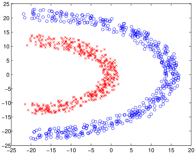
c. Half kernel

d. Cluster in cluster

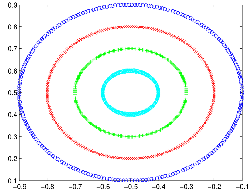
e. Dartboard

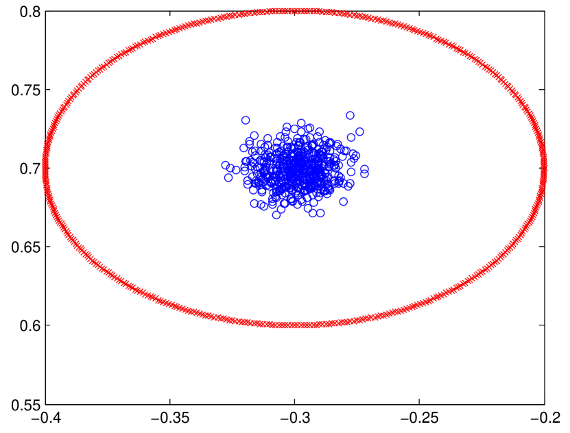
f. Donut

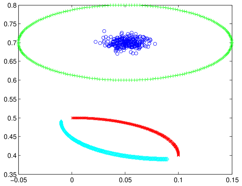
g. Donutcurves

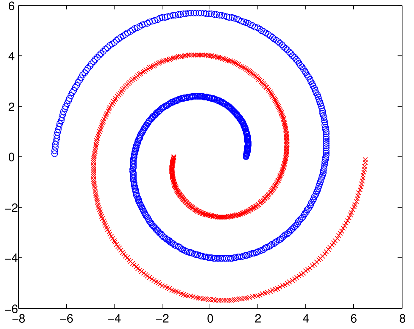
h. Spiral1

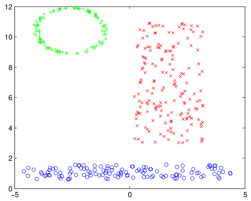
i. 3MC

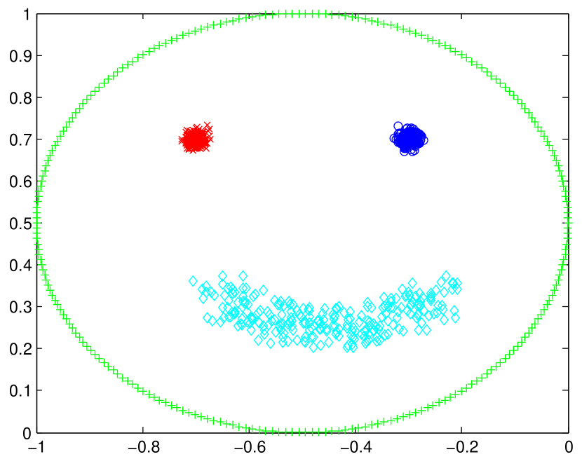
j. Smile

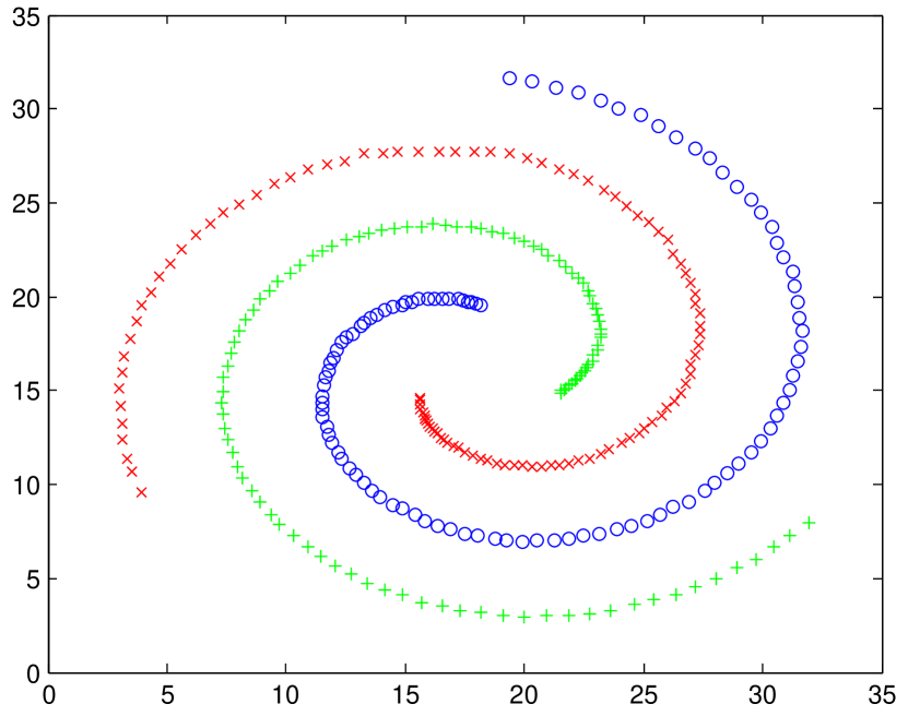
k. Spiral2

l. Zelnik

Figure B.1: CRL on some standard clustering benchmarks. The obtained clusters are labeled in difference colors.

We then created more clusters and increased dimensions to make the problems more challenging. Specifically, a new dataset Zelnik^∗ with $q^{*}=12,m=50$ was created by shifting the data points of Zelnik four times followed by (right)multiplying the data matrix by a random Gaussian matrix. Similarly, we constructed a new dataset Donutcurves^∗ with $q^{*}=12$ and $m=100$. In comparing spectral clustering and kernel CRL, we considered two standard types of the similarity matrix $\boldsymbol{W}$, one based on Gaussian similarities, the other based on mutual $k$-nearest neighbor graph with $k=20$; see von Luxburg, (2007) for details. The normalized graph Laplacian is then $\boldsymbol{L}=\boldsymbol{I}-\boldsymbol{D}^{-1/2}\boldsymbol{W}\boldsymbol{D}^{-1/2}$. Table B.2 and Table B.3 summarize the results with each experiment repeated $50$ times. In these tough situations, no algorithm gives perfect clustering, but CRL clearly outperforms spectral clustering and again, performing a further dimension reduction is still possible and helpful.

Table B.2: Clustering accuracy on two enlarged benchmarks using Gaussian similarity matrices.

Dataset	Zelnik∗	Donutcurves∗
$(n,m,q^{*})$	$(1064,50,12)$	$(3000,100,12)$
spectral clustering	0.70	0.71
CRL ($r=q$)	0.74	0.92
CRL ($r=0.75q$)	0.76	0.94

Table B.3: Clustering accuracy on two enlarged benchmarks using mutual $20$-nearest neighbor based similarity matrices.

Dataset	Zelnik∗	Donutcurves∗
$(n,m,q^{*})$	$(1064,50,12)$	$(3000,100,12)$
Spectral clustering	0.68	0.68
CRL ($r=q$)	0.72	0.89
CRL ($r=0.75q$)	0.73	0.91

B.3 Community detection

We performed systematic experiments on some community detection benchmarks. Although CRL is not specially designed to solve this kind of problem, it has impressive performance even compared with some state-of-the-art methods.

This parts uses two popular network community detection benchmarks, the GN benchmark (Girvan and Newman,, 2002; Newman and Girvan,, 2004) and the LFR benchmark (Lancichinetti et al.,, 2008) to show the performance of CRL in comparison with some widely used community detection methods. In the GN benchmark, $n$ nodes are divided into $q$ homogeneous clusters of size $s$. The parameters $z_{in}$ and $z_{out}$ control the internal degree and the external degree of each node, respectively. We set $n=1000$, $q=20$, $s=50$, $z_{in}=15$ and $z_{out}=30$, where $z_{out}$ doubles the size of $z_{in}$ to increase the difficulty in clustering. In the LFR benchmark, both the degree distribution and community size distribution follow power laws to generate a network with more heterogeneities. The parameters are: $n$, the number of nodes, $d$, the average degree, $d_{\max}$, the maximum node degree, $\mu$, the mixing ratio, $\beta$, the power index of community size, $\gamma$, the power index of node degree and $c_{\min}$ ($c_{\max}$), the minimum (maximum) community size. In our experiment, we used $n=1000$, $d=15$, $d_{\max}=50$, $c_{\min}=20$, $c_{\max}=50$, $\gamma=2$, $\beta=1$, and varied the crucial parameter $\mu$ from $0.1$ to $0.9$. The metrics include, in addition to CA and RI, the normalized mutual information (NMI) (Danon et al.,, 2005). Both RI and NMI have range $[0,1]$, and the larger the value is, the more accurate the tested algorithm. The comparison community detection methods include the Newman-Girvan method (Newman and Girvan,, 2004), Hespanha’s algorithm (Hespanha,, 2004), the method by Dannon et al (Danon et al.,, 2006) and AMOS (Chen et al.,, 2016). In all algorithms, we set $q$ to be $q^{*}$ to remove the influence of ad-hoc tuning schemes. The results on the GN benchmark are reported in Table B.4. For the LFR benchmark, we plot the performance of each algorithm as a function of the mixing parameter $\mu$ in Figure B.2. In summary, although CRL is not particularly designed for network community detection, it does a decent job on the standard benchmarks.

Table B.4: GN benchmark: clustering performance in terms of CA, RI, NMI

	CA	RI	NMI
Newman-Girvan	0.34	0.77	0.39
Hespanha	0.30	0.91	0.29
Danon et al.	0.36	0.89	0.37
AMOS	0.67	0.92	0.65
CRL	0.96	0.98	0.94

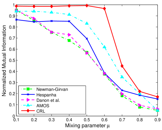
Figure B.2: LFR benchmark: clustering performance of different algorithms evaluated by NMI, as the mixing parameter $\mu$ varies from 0.1 to 0.9.

B.4 Model misspecification

This part performs simulations to test the performance of CRL and some other methods when model misspecification occurs. The $n$ observations of the responses and predictors are independently generated according to $\boldsymbol{y}_{i}=\boldsymbol{B}^{*T}\tilde{\boldsymbol{x}}_{i}+\boldsymbol{e}_{i}$, where $\boldsymbol{y}_{i}\in\mathbb{R}^{m}$, $\tilde{\boldsymbol{x}}_{i}\in\mathbb{R}^{p}$, and $\boldsymbol{e}_{i}$ has standard normal entries ($\mu=0,\sigma=1$). In the experiment, $n=100,p=50,m=25$, and all rows of the design follow a multivariate normal distribution with a covariance matrix $\boldsymbol{\Sigma}=[\tau^{|i-j|}]$ where $\tau=0.2$.

To study the effect of model misspecification, we generate the true coefficient matrix $\boldsymbol{B}^{*}$ through $\boldsymbol{B}^{\circ}$ and $\sigma_{B}$ as follows. First, $\boldsymbol{B}^{\circ}=\boldsymbol{B}_{1}\boldsymbol{B}_{2}^{T}$, where $\boldsymbol{B}_{1}\in\mathbb{R}^{p\times r},\boldsymbol{B}_{2}\in\mathbb{R}^{m\times r}$. The entries of $\boldsymbol{B}_{2}$ are standard Gaussian, and each row $\boldsymbol{b}_{j}$ ($1\leq j\leq p$) of $\boldsymbol{B}_{1}$ is drawn from an equally weighted mixture distribution: $\boldsymbol{b}_{j}$ is zero or has an elementwise distribution $N(k,1)$, $1\leq k\leq q-1$. We set $q=10,r=5$, and so $\boldsymbol{B}^{\circ}$ has about 10% rows being zero, and satisfies $\|\boldsymbol{B}^{\circ}\|_{2,\mathcal{C}}=10$, $\mbox{rank}(\boldsymbol{B}^{\circ})=5$. Next, we obtain $\boldsymbol{B}^{*}\in\mathbb{R}^{p\times m}$, consisting of 1,250 entries, by adding additional noise $N(0,\sigma_{B}^{2})$ to $\boldsymbol{B}^{\circ}$ in an elementwise fashion. Clearly, when $\sigma_{B}=0$, the true coefficient matrix has sparsity, row-wise equisparsity, and low rank, but the structural parsimony is easily destroyed by a nonzero $\sigma_{B}$.

The methods for comparison include LASSO, group LASSO (G-LASSO), reduced rank regression (RRR), fused LASSO (F-LASSO), and CRL. All the algorithmic parameters are set to their default values. Our goal in this experiment is to make a fair comparison of all methods and understand the true potential of each; to remove the influence of various schemes for regularization parameter tuning, we pick the estimate along the solution path that gives the smallest validation error, evaluated on a large independent validation dataset with 10,000 observations. We varied the misspecification level $\sigma_{B}$ from $0$ to $0.12$ and repeated the experiment in each setup for 20 times. Table B.5 reports the median estimation error $\|\hat{\boldsymbol{B}}-\boldsymbol{B}^{*}\|_{F}^{2}$ (denoted by $\mbox{Err}^{(e)}$), as well as the predictor error $\|\boldsymbol{Y}_{tst}-\boldsymbol{X}_{tst}\hat{\boldsymbol{B}}\|_{F}^{2}/n_{tst}-m$ over the test dataset $(\boldsymbol{Y}_{tst},\boldsymbol{X}_{tst})$ with $n_{tst}=10\mbox{,}000$ observations (denoted by $\mbox{Err}^{(p)}$).

Table B.5: Performance comparison between LASSO, group LASSO (G-LASSO), reduced rank regression (RRR), fused LASSO (F-LASSO), and CRL, based on estimation error $\mbox{(Err}^{(e)}$) and prediction error ($\mbox{Err}^{(p)}$), when varying the model misspecification level $\sigma_{B}$

		$\sigma_{\scriptscriptstyle B}\!=\!0$			$\sigma_{\scriptscriptstyle B}\!=\!0.04$			$\sigma_{\scriptscriptstyle B}\!=\!0.08$			$\sigma_{\scriptscriptstyle B}\!=\!0.12$			$\sigma_{\scriptscriptstyle B}\!=\!0.16$
		$\mbox{Err}^{(e)}$	$\mbox{Err}^{(p)}$		$\mbox{Err}^{(e)}$	$\mbox{Err}^{(p)}$		$\mbox{Err}^{(e)}$	$\mbox{Err}^{(p)}$		$\mbox{Err}^{(e)}$	$\mbox{Err}^{(p)}$		$\mbox{Err}^{(e)}$	$\mbox{Err}^{(p)}$
LASSO		22.6	20.9		22.8	21.0		23.0	21.4		23.6	21.9		23.9	22.1
G-LASSO		22.7	21.4		23.0	21.7		23.8	22.4		25.1	23.1		26.0	24.3
[1pt/2pt] RRR		6.58	6.21		8.17	7.79		13.1	12.6		21.0	20.1		25.3	23.8
[1pt/2pt] F-LASSO		22.7	21.6		23.0	21.7		23.1	21.9		23.6	22.3		24.1	22.5
[1pt/2pt] CRL		2.12	2.14		4.15	4.14		10.2	10.1		20.1	19.5		25.1	23.7

First, as $\sigma_{B}=0$, although a total of 10% of authentic coefficients are zero, the sparsity (or group-wise sparsity) is still inadequate for LASSO or group LASSO to show a clear advantage over the other methods. Fused LASSO, which imposes sparsity on successive coefficient differences $|b_{j+1,k}-b_{j,k}|$ ($1\leq j<p,1\leq k\leq m$) in addition to performing variable selection, failed to capture all the equi-sparsity, largely because it assumes that the features are already grouped and ordered to have the associated coefficients equal in consecutive blocks (which is however impractical in most real life applications).

According to the table, when $\sigma_{B}$ is large enough (say, $\sigma_{B}\geq 0.16$) to break the parsimony assumptions, all methods (unsurprisingly) yield very complex models with large errors, the saturated model being the extreme. But the low-rank based RRR, and notably CRL, outperformed the other methods by a large margin when the large coefficient matrix only has approximate low rank and equisparsity. This was evidenced as long as $\sigma_{B}\leq 0.1$ by more systematic experiments (not all shown in the table). The excellent performance of CRL in these cases verifies the oracle-inequality type analysis mentioned at the end of Section 3.2.

References

- Agresti, (2012) Agresti, A. (2012). Categorical Data Analysis. Wiley Series in Probability and Statistics. Wiley.
- Arthur and Vassilvitskii, (2007) Arthur, D. and Vassilvitskii, S. (2007). K-means++: The advantages of careful seeding. In Proceedings of the Eighteenth Annual ACM-SIAM Symposium on Discrete Algorithms, pages 1027–1035. Society for Industrial and Applied Mathematics.
- Bachem et al., (2016) Bachem, O., Lucic, M., Hassani, S. H., and Krause, A. (2016). Fast and provably good seedings for K-means. In Proceedings of the 30th International Conference on Neural Information Processing Systems, NIPS’16, pages 55–63. Curran Associates Inc.
- Bickel et al., (2009) Bickel, P. J., Ritov, Y., and Tsybakov, A. B. (2009). Simultaneous analysis of Lasso and Dantzig selector. The Annals of Statistics, 37:1705–1732.
- Bregman, (1967) Bregman, L. (1967). The relaxation method of finding the common point of convex sets and its application to the solution of problems in convex programming. USSR Computational Mathematics and Mathematical Physics, 7(3):200 – 217.
- Breiman et al., (1984) Breiman, L., Friedman, J., Stone, C., and Olshen, R. (1984). Classification and Regression Trees. Taylor & Francis, Monterey, CA.
- Bunea et al., (2011) Bunea, F., She, Y., and Wegkamp, M. (2011). Optimal selection of reduced rank estimators of high-dimensional matrices. The Annals of Statistics, 39:1282–1309.
- Cai et al., (2005) Cai, D., He, X., and Han, J. (2005). Document clustering using locality preserving indexing. IEEE Transactions on Knowledge and Data Engineering, 17(12):1624–1637.
- Candès and Tao, (2007) Candès, E. and Tao, T. (2007). The Dantzig selector: Satistical estimation when p is much larger than n. The Annals of Statistics, pages 2313–2351.
- Candès and Plan, (2011) Candès, E. J. and Plan, Y. (2011). Tight oracle bounds for low-rank matrix recovery from a minimal number of random measurements. IEEE Transactions on Information Theory, 57(4):2342–2359.
- Chang and Yeung, (2008) Chang, H. and Yeung, D.-Y. (2008). Robust path-based spectral clustering. Pattern Recognition, 41(1):191–203.
- Chen et al., (2016) Chen, P.-Y., Gensollen, T., and Hero III, A. O. (2016). Amos: An automated model order selection algorithm for spectral graph clustering. arXiv preprint arXiv:1609.06457.
- Chi and Lange, (2015) Chi, E. C. and Lange, K. (2015). Splitting methods for convex clustering. Journal of Computational and Graphical Statistics, 24:4:994–1013.
- Chun and Keleş, (2010) Chun, H. and Keleş, S. (2010). Sparse partial least squares regression for simultaneous dimension reduction and variable selection. Journal of the Royal Statistical Society: Series B (Statistical Methodology), 72(1):3–25.
- Danon et al., (2006) Danon, L., Díaz-Guilera, A., and Arenas, A. (2006). The effect of size heterogeneity on community identification in complex networks. Journal of Statistical Mechanics: Theory and Experiment, 2006(11):P11010.
- Danon et al., (2005) Danon, L., Diaz-Guilera, A., Duch, J., and Arenas, A. (2005). Comparing community structure identification. Journal of Statistical Mechanics: Theory and Experiment, 2005(09):P09008.
- Donoho and Johnstone, (1994) Donoho, D. L. and Johnstone, J. M. (1994). Ideal spatial adaptation by wavelet shrinkage. Biometrika, 81(3):425–455.
- Girvan and Newman, (2002) Girvan, M. and Newman, M. E. (2002). Community structure in social and biological networks. Proceedings of the National Academy of Sciences, 99(12):7821–7826.
- Götze et al., (2021) Götze, F., Sambale, H., and Sinulis, A. (2021). Concentration inequalities for polynomials in -sub-exponential random variables. Electronic Journal of Probability, 26:1–22.
- Hastie et al., (2009) Hastie, T., Tibshirani, R., and Friedman, J. (2009). The Elements of Statistical Learning. Springer-Verlag, New York, 2nd edition.
- Hespanha, (2004) Hespanha, J. P. (2004). An efficient matlab algorithm for graph partitioning. Santa Barbara, CA, USA: University of California.
- Izenman, (1975) Izenman, A. J. (1975). Reduced-rank regression for the multivariate linear model. Journal of Multivariate Analysis, 5(2):248–264.
- Jain and Law, (2005) Jain, A. and Law, M. (2005). Data clustering: A user’s dilemma. Pattern Recognition and Machine Intelligence, pages 1–10.
- Johnstone and Lu, (2009) Johnstone, I. M. and Lu, A. Y. (2009). On consistency and sparsity for principal components analysis in high dimensions. Journal of the American Statistical Association, 104(486):682–693.
- Jørgensen, (1987) Jørgensen, B. (1987). Exponential Dispersion Models. Journal of the Royal Statistical Society. Series B, 49(2):127–145.
- Koltchinskii et al., (2011) Koltchinskii, V., Lounici, K., and Tsybakov, A. B. (2011). Nuclear-norm penalization and optimal rates for noisy low-rank matrix completion. The Annals of Statistics, 39(5):2302 – 2329.
- Lambert et al., (2010) Lambert, J.-P., Fillingham, J., Siahbazi, M., Greenblatt, J., Baetz, K., and Figeys, D. (2010). Defining the budding yeast chromatin-associated interactome. Molecular Systems Biology, 6(1):448.
- Lancichinetti et al., (2008) Lancichinetti, A., Fortunato, S., and Radicchi, F. (2008). Benchmark graphs for testing community detection algorithms. Physical Review E, 78(4):046110.
- Lounici et al., (2011) Lounici, K., Pontil, M., Tsybakov, A. B., and van de Geer, S. (2011). Oracle inequalities and optimal inference under group sparsity. The Annals of Statistics, 39:2164–2204.
- Lovász and Plummer, (2009) Lovász, L. and Plummer, M. D. (2009). Matching Theory, volume 367. AMS Chelsea Publishing: An Imprint of the American Mathematical Society.
- Newman and Girvan, (2004) Newman, M. E. and Girvan, M. (2004). Finding and evaluating community structure in networks. Physical review E, 69(2):026113.
- Pan and Heitman, (2000) Pan, X. and Heitman, J. (2000). Sok2 regulates yeast pseudohyphal differentiation via a transcription factor cascade that regulates cell-cell adhesion. Molecular and Cellular Biology, 20(22):8364–8372.
- Pellikaan et al., (2017) Pellikaan, R., Wu, X.-W., Bulygin, S., and Jurrius, R. (2017). Codes, Cryptology and Curves with Computer Algebra. Cambridge University Press, Cambridge, 1st edition.
- Rand, (1971) Rand, W. M. (1971). Objective criteria for the evaluation of clustering methods. Journal of the American Statistical association, 66(336):846–850.
- Rennie and Dobson, (1969) Rennie, B. and Dobson, A. (1969). On Stirling numbers of the second kind. Journal of Combinatorial Theory, 7(2):116 – 121.
- Rockafellar, (1970) Rockafellar, R. T. (1970). Convex Analysis. Princeton University Press, Princeton, NJ.
- Rousseeuw and Driessen, (1999) Rousseeuw, P. J. and Driessen, K. V. (1999). A fast algorithm for the minimum covariance determinant estimator. Technometrics, 41(3):212–223.
- Sambale, (2020) Sambale, H. (2020). Some notes on concentration for -subexponential random variables. arXiv preprint arXiv:2002.10761.
- She, (2010) She, Y. (2010). Sparse regression with exact clustering. Electronic Journal of Statistics, 4:1055–1096.
- She, (2017) She, Y. (2017). Selective factor extraction in high dimensions. Biometrika, 104(1):97–110.
- She et al., (2020) She, Y., Tang, S., and Zhang, Q. (2020). Indirect Gaussian Graph Learning beyond Gaussianity. IEEE Transactions on Network Science and Engineering, 7:918–929.
- She and Tran, (2019) She, Y. and Tran, H. (2019). On cross-validation for sparse reduced rank regression. Journal of the Royal Statistical Society: Series B, 81:145–161.
- She et al., (2021) She, Y., Wang, Z., and Jin, J. (2021). Analysis of generalized Bregman surrogate algorithms for nonsmooth nonconvex statistical learning. The Annals of Statistics, 49(6):3434–3459.
- Szarek, (1982) Szarek, S. J. (1982). Nets of Grassmann manifold and orthogonal groups. In Proceedings of Banach Spaces Workshop, volume 169, pages 169–185.
- Tibshirani et al., (2005) Tibshirani, R., Saunders, M., Rosset, S., Zhu, J., and Knight, K. (2005). Sparsity and smoothness via the fused LASSO. Journal of the Royal Statistical Society: Series B (Statistical Methodology), 67(1):91–108.
- Tsybakov, (2008) Tsybakov, A. B. (2008). Introduction to Nonparametric Estimation. Springer Publishing Company, Incorporated, New York, 1st edition.
- van der Vaart and Wellner, (1996) van der Vaart, A. and Wellner, J. (1996). Weak Convergence and Empirical Processes: With Applications to Statistics. Springer.
- van Lint, (1982) van Lint, J. H. (1982). Introduction to Coding Theory. Springer-Verlag, Berlin, Heidelberg.
- von Luxburg, (2007) von Luxburg, U. (2007). A tutorial on spectral clustering. Statistics and Computing, 17(4):395–416.
- Wainwright and Jordan, (2008) Wainwright, M. J. and Jordan, M. I. (2008). Graphical models, exponential families, and variational inference. Foundations and Trends in Machine Learning, 1:1–305.
- Yuan and Lin, (2006) Yuan, M. and Lin, Y. (2006). Model selection and estimation in regression with grouped variables. Journal of the Royal Statistical Society: Series B (Statistical Methodology), 68(1):49–67.
- Zhang and Xia, (2009) Zhang, C. and Xia, S. (2009). K-means clustering algorithm with improved initial center. In Proceedings of the 2009 Second International Workshop on Knowledge Discovery and Data Mining, pages 790–792. IEEE.