Interpretable Data-Based Explanations for Fairness Debugging

Abstract.

A wide variety of fairness metrics and eXplainable Artificial Intelligence (XAI) approaches have been proposed in the literature to identify bias in machine learning models that are used in critical real-life contexts. However, merely reporting on a model’s bias, or generating explanations using existing XAI techniques is insufficient to locate and eventually mitigate sources of bias. We introduce Gopher, a system that produces compact, interpretable and causal explanations for bias or unexpected model behavior by identifying coherent subsets of the training data that are root-causes for this behavior. Specifically, we introduce the concept of causal responsibility that quantifies the extent to which intervening on training data by removing or updating subsets of it can resolve the bias. Building on this concept, we develop an efficient approach for generating the top-$k$ patterns that explain model bias that utilizes techniques from the machine learning (ML) community to approximate causal responsibility and uses pruning rules to manage the large search space for patterns. Our experimental evaluation demonstrates the effectiveness of Gopher in generating interpretable explanations for identifying and debugging sources of bias.

1. Introduction

Machine learning (ML) is being increasingly applied to decision-making in sensitive domains such as finance, healthcare, crime prevention and justice management. Although it has the potential to overcome undesirable aspects of human decision-making, concern continues to mount that its opacity perpetuates systemic biases and discrimination reflected in training data (fb-housing, ; self-driving-cars, ; 10.1145/2702123.2702520, ). This concern has caused increasing regulations and demands for generating human understandable explanations for the behavior of ML algorithms— an issue addressed by the rapidly growing field of eXplainable Artificial Intelligence (XAI); see (molnar2020interpretable, ) for a recent survey.

The development of XAI methods is motivated by technical, social and ethical objectives (kasirzadeh2021reasons, ; datta2016algorithmic, ; binns2018s, ; lepri2018fair, ; kemper2019transparent, ) including: (1) providing users with actionable insights to change the results of algorithms in the future, (2) facilitating the identification of sources of harms such as bias and discrimination, and (3) providing the ability to debug ML algorithms and models by identifying errors or biases in training data that result in adverse and unexpected behavior.

Most XAI research to date has focused on generating feature-based explanations, which quantify the extent to which input feature values contribute to an ML model’s predictions. In this direction, methods based on feature importance quantification (lipovetsky2001analysis, ; vstrumbelj2014explaining, ; lundberg2017unified, ; lundberg2018consistent, ; datta2016algorithmic, ; merrick2019explanation, ; frye2019asymmetric, ; aas2019explaining, ), surrogate models, causal and counterfactual methods (lundberg2017unified, ; ribeiro2016should, ; ribeiro2018anchors, ), and logic-based approaches  (shih2018symbolic, ; ignatiev2020towards, ; darwiche2020reasons, ) are designed to reveal the dependency patterns between the input features and output of ML algorithms. These methods differ in terms of whether they address correlational, causal, counterfactual or contrastive patterns. While such explanations satisfy the aforementioned objectives (1) and (2) if we only consider the test data as a source of bias, they fall short in generating diagnostic explanations that let users trace unexpected or discriminatory algorithmic behavior back to its training data. Hence, they fail to satisfy objective (3) if the training data is the source of the bias. Indeed, information solely about output-input feature dependency is insufficient to explain discriminatory and unexpected algorithmic decisions in terms of data errors and biases introduced during data collection and preparation. While a feature-based explanation can identify which features of a test data point are correlated with a misprediction or bias, it does not explain why the model exhibits this bias. To explain such behavior, we must trace the bias back to the data used to train the model. For example, feature-based approaches cannot generate explanations of the form: “The primary source of gender bias for this classifier, which decides about loan applications, is its training data which exhibits bias against the credit scores of unmarried females who are house owners.”

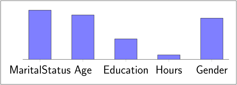
(a) Feature-based explanations

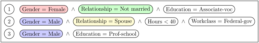
(b) Top-k explanations generated by Gopher

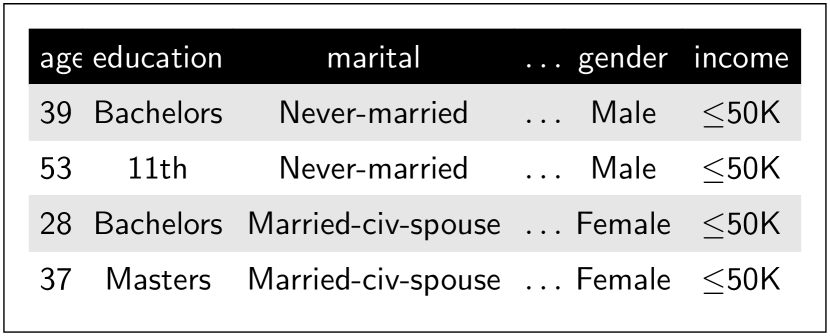
(c) Instance-based explanations

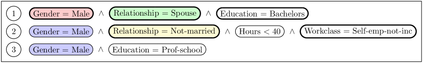
(d) Update-based explanations for the corresponding top-k explanations

Figure 1. An overview of explanations generated by XAI approaches for an ML algorithm built using the UCI Adult dataset (see Section 6 for details), which predicts if an individual earns $\geq 50$K/year. (a) Feature-based explanations rank attributes in descending order of importance toward model behavior. (c) Instance-based explanations output a list of data points most responsible for model behavior. Gopher generates two kinds of explanations: (b) top-$k$ explanations identify the patterns most causally responsible for model bias, and (d) updates to the top-k explanations that reduce the model’s bias by the most.

In this paper, we take the first step toward developing a framework for generating diverse, compact and interpretable training data-based explanations that identity which parts of the training data are responsible for an unexpected and discriminatory behavior of an ML model. Specifically, we introduce Gopher, a system that finds patterns which compactly describe cohesive sets of training data points that, when eliminated, reduce the bias of the model. In other words, if the ML algorithm had been trained on the modified training data, it would not have exhibited the unexpected or undesirable behavior or would have exhibited this behavior to a lesser degree. Explanations generated by our framework, which complement existing approaches in XAI, are crucial for helping system developers and ML practitioners to debug ML algorithms by identifying data errors and bias in training data, such as measurement errors and misclassifications (gianfrancesco2018potential, ; jacobs2021measurement, ; wang2021fair, ), data imbalance (farrand2020neither, ), missing data and selection bias (fernando2021missing, ; martinez2019fairness, ; mehrabi2019survey, ), covariate shift (rezaei2020robust, ; singh2021fairness, ), technical biases introduced during data preparation (Stoyanovich2020ResponsibleDM, ), and poisonous data points injected through adversarial attacks (solans2020poisoning, ; jagielski2020subpopulation, ; mehrabi2020exacerbating, ; goel2021importance, ). It is known in the algorithmic fairness literature that information about the source of bias is critically needed to build fair ML algorithms because none of the current bias mitigation solutions fits all situations (singh2021fairness, ; wang2021fair, ; farrand2020neither, ; goel2021importance, ; Fu2020AIAA, ).

We use the example shown below to illustrate the difference between feature- and data-based techniques, that explain bias based on the contribution of a subset of the training data.

Example 1.1.

Consider a classifier that predicts whether individuals described by their attributes (such as gender, education level, marital status, working hours, etc.) earn more than $50$K a year. A system developer uses the classifier to predict the income of individuals and, while analyzing the results, finds an unexpected negative result (earning less than $50$K) for a female user:

age	education	marital	workclass	race	gender	hours
34	Bachelors	Never-married	Private	Black	Female	40

Based on her education ($\texttt{{education}}=\text{Bachelors}$), marital status ($\texttt{{marital}}=\text{Never-married}$), (age=$34$), and other features, this user should be classified as earning more than $50$K. Upon closer examination, the developer realizes that the classifier violates the commonly used fairness metric of statistical parity with respect to the protected group $\texttt{{gender}}=Female$. Statistical parity requires that the probability of being classified as the positive class (earning more than $50$K in our example) is the same for individuals from the protected group as it is for individuals from the privileged group (we present fairness definitions in Section 2).

The developer uses an existing XAI package, such as LIME (ribeiro2016should, ) or SHAP (lundberg2017unified, ), to explain the algorithm’s output for the user and learns that the user’s gender and unmarried status were most responsible for the faulty prediction. We show examples of such explanations in Figure 1(a) and (c). These explanations, however, do not help the developer identify the source of the model’s bias. In contrast, Gopher identifies cohesive subsets of the training data that are most responsible for the bias and compactly describes the subsets using patterns that are conjunctions of predicates. Figure 1(c) shows the top-3 explanations Gopher produces. Pattern $\phi_{2}$ states that a sub-population that strongly impacts model bias is male spouses who work in the federal government for less than 40 hours per week. Indeed, in the Adult Income dataset (see Section 6), this subpopulation is the major source of gender bias, because it reports household income; hence, due to the bias in data collection, married males becomes highly correlated with high-income. In addition to producing such explanations, Gopher also identifies homogeneous updates for sub-populations that can maximally improve model bias. Figure 1(d) shows one such update (with bold outline). For instance, model bias would significantly decline if we changed relationship status from “Spouse” to “Not married” and Workclass from federal employee to self-employed in the subset of the training data corresponding to $\phi_{2}$. Such updates mean that our approach not only identifies which subsets of training data are responsible for the bias, but also which features of the data points in these subsets are responsible.

Root causes and responsibility. Our first contribution is to formalize root causes of bias and the causal responsibility of a subset of the training data for the bias of an ML model. Responsibility is measured as the difference between the bias of the original model and that of a new model trained on the modified training data, obtained by either removing or updating the subset. We define data-based explanations for bias as the top-k subsets of the training data that have the highest causal responsibility toward model bias.

Pattern-based explanations. Such “raw explanations” based on subsets of data points may overwhelm rather than inform end-users. More compact and coherent descriptions are needed. Furthermore, sources of bias and discrimination in training data are typically not randomly distributed across different sub-populations; rather they manifest systematic errors in data collection, selection, feature engineering, and curation (gianfrancesco2018potential, ; jacobs2021measurement, ; wang2021fair, ; fernando2021missing, ; martinez2019fairness, ; mehrabi2019survey, ; parikh2019addressing, ). In other words, more often than not, certain cohesive training data subsets are responsible for bias. Our system generates explanations in terms of compact patterns expressed as first-order predicates that describe homogenous training data subsets. By identifying commonalities within training data subsets, which are the main contributors to model bias, such explanations unearth the root causes of bias. To ensure that the generated explanations are diverse, our system filters explanations that refer to similar subsets of training data.

Computational challenges. Computing such explanations is challenging for two main reasons. First, computing the causal responsibility of a given subset of data requires retraining the ML model, which is expensive. Second, it is computationally prohibitive to explore all possible subsets of training data to identify the top-$k$ explanations. To address the first challenge, we trace the model’s predictions through its learning algorithm back to the training data. To do so, we approximate the change in model parameters by using either influence functions (cook-influence, ) or by assuming that the updated model parameters can be computed by applying a single gradient decent step to the original model. First-order (FO) approximations of influence functions have recently been proven useful in ML model debugging (pmlr-v70-koh17a, ) by identifying the top-k training data points responsible for model mis-predictions. However, they do not effectively capture the ground truth influence of training data subsets because of correlations between data points. To better approximate the change in model parameters, we utilize second-order (SO) influence functions, which were shown to better correlate with ground truth subset influence (icml2020_4261, ). While even SO influence functions can provide relatively poor estimates of the influence of large portions of the training data, the approximation error of SO influence functions is typically much better for coherent sets of data points as described by our patterns. To address the second challenge, we develop a lattice-based search algorithm based on ideas from frequent itemset mining (10.5555/645920.672836, ) to discover frequent patterns. Our algorithm identifies coarse-grained subsets of training data that are influential and successively refines them to discover smaller influential subsets. We introduce a novel quality metric for explanations, and optimizations that further prune the search space and efficiently generate the top-k explanations.

Update-based explanations. Gopher is unique in that, in addition to generating explanations in terms of data removal, it also considers explanations based on updating data points. This aspect of Gopher is motivated by the observation that not all features of a data point are erroneous and responsible for the bias. To identify an update that mitigates bias, we search for a homogeneous perturbation of some of the feature of the training data points described by a pattern (explanation) that leads to a maximal reduction in model bias. By homogeneous we mean that all data points in the subset are updated using the same perturbation vector, e.g., we change the marital status from never-married to divorced. We formulate the problem of computing update-based explanations as a constrained optimization problem that searches for a homogeneous update to a subset of training data in order to maximize bias reduction, and we solve it using projected gradient descent (Bubeck2015ConvexOA, ).

We make the following contributions:

• We formalize interventions on training data that remove or update training data points and estimate their effect on ML model bias. Utilizing intervention, we define predicate-based causal explanations to identify training data subsets that contribute significantly to ML model bias (Section 3).

• We approximate the effect of training data deletion on model bias (Section 4.1) to avoid expensive retraining.

• We propose a principled approach for generating top-k explanations based on frequent pattern mining and use pruning techniques to reduce the size of the search space (Section 4.2).

• We introduce update-based, actionable explanations. These explanations identify not only which parts of the training data are responsible for the bias but also how to reduce or ”repair” the bias. We formalize the problem of finding the most effective explanation as a constrained optimization problem that maximizes bias reduction. We propose a new algorithm based on projected gradient descent to determine the best homogeneous update for a responsible training data subset (Section 5).

• We conducted extensive experiments using real-world datasets to evaluate: (1) the end-to-end performance of Gopher, (2) the accuracy of influence estimation techniques, and (3) the quality and interpretability of explanations (Section 6). We show that Gopher generates explanations that are consistent with insights from existing literature.

2. Background and Assumptions

We now present pertinent background information on classification and algorithmic fairness.

Classification. We consider the problem of binary classification, which is the focus of most literature on algorithmic fairness. Consider a training dataset of $n$ examples ${\mathbf{D}}=\{{\mathbf{z}}_{i}=({\mathbf{x}}_{i},y_{i})\}_{i=1}^{n}$, with domain $\textsc{Dom}({\mathbf{X}})\times\textsc{Dom}(Y)$, drawn from an unknown data distribution $\mathcal{D}$, where ${\mathbf{X}}$ denotes a set of discrete and continuous features and $Y=\{0,1\}$ is a binary label to be predicted. Here, the goal is to find a classifier $f\mathrel{\mathop{\ordinarycolon}}\textsc{Dom}({\mathbf{X}})\to\hat{Y}$ that associates each data point ${\mathbf{x}}$ with a predicted label $\hat{y}\in\hat{Y}=\{0,1\}$ that maximizes accuracy $E_{{\mathbf{x}},y\sim\mathcal{D}}[\mathbb{1}(f({\mathbf{x}})=y)]$, i.e., the expectation of the fraction of data points from the unknown data distribution $\mathcal{D}$ that are correctly predicted by $f$. Note that since we have access to only a sample ${\mathbf{D}}$ of $\mathcal{D}$, model performance is determined over the training data as a substitute for calculating $E_{{\mathbf{x}},y\sim\mathcal{D}}[\mathbb{1}(f({\mathbf{x}})=y)]$. Typically, $f(.)$ is a member of a family of functions $f_{\theta}$ that are parameterized by $\theta$ with domain $\Theta$. A learning algorithm $\mathcal{A}$ uses ${\mathbf{D}}$ and learns parameters $\theta^{*}\in\Theta$ that maximize the empirical accuracy $\sum_{i=1}^{n}\mathbb{1}(f_{\theta}({\mathbf{x}})=y)$. Learning algorithms typically use some loss function $L({\mathbf{z}},\theta)$ and minimize the empirical loss $\mathcal{L}({\mathbf{D}},\theta)=\frac{1}{n}\sum_{i=1}^{n}L({\mathbf{z}},\theta)$. We denote the optimal parameters $\theta^{*}$ of a classifier as $\theta$ when it is clear from the context. Throughout this paper, we consider learning algorithms that use a loss function $\mathcal{L}(\theta)$ that is twice-differentiable, which covers classification algorithms such as logistic regression (sklearn, ), support vector machines (SVM) (sklearn, ), and feedforward neural networks (fastai, ).

Algorithmic fairness. Consider a binary classifier $f_{\theta}$ with output $\hat{Y}$ and a protected attribute $S\in{\mathbf{X}}$, such as gender or race. Without loss of generality, we interpret $\hat{Y}=1$ as a favorable (positive) prediction and $\hat{Y}=0$ as an unfavorable (negative) prediction. To simplify the exposition, we assume $\textsc{Dom}(S)=\{0,1\}$, where $S=1$ indicates a privileged and $S=0$ indicates a protected group (e.g., males and non-males, respectively). Algorithmic fairness aims to ensure that the classifier $f$ makes fair predictions devoid of discrimination with respect to the protected attribute(s). Many fairness definitions have been proposed to quantify the bias of a binary classifier (see (10.1145/3194770.3194776, ) for a recent survey). The best-known ones are based on associative relationships between the protected attribute and the classifier’s outcome. These definitions are unlike causal notions of fairness, which incorporate background knowledge about the underlying data-generative process and define fairness in terms of the causal influence of the protected attribute on the classifier’s outcome (kusner2017counterfactual, ; kilbertus2017avoiding, ; nabi2018fair, ; salimi2019interventional, ). We focus on three of the most widely used associational notions of fairness:

Statistical parity requires an algorithm to classify both the protected and privileged group with the same probability:

$${\tt\mathrm{Pr}}(\hat{Y}=1|S=1)={\tt\mathrm{Pr}}(\hat{Y}=1|S=0).$$

Equal opportunity requires both the protected and privileged group to have the same true positive rate:

$${\tt\mathrm{Pr}}(\hat{Y}=1|Y=1,S=1)={\tt\mathrm{Pr}}(\hat{Y}=1|Y=1,S=0).$$

Predictive parity requires that both protected and privileged groups have the same predicted positive value (PPV), i.e., correct positive predictions have to be independent of the protected attribute:

$${\tt\mathrm{Pr}}(Y=1|\hat{Y}=1,S=1)={\tt\mathrm{Pr}}(Y=1|\hat{Y}=1,S=0).$$

In practice, these fairness notions are often evaluated by estimating the probabilities on a test dataset ${\mathbf{D}}_{test}$. Note that our techniques also work for other associational and causal notions of fairness.

3. Problem Statement

In this section, we introduce root causes for bias and define data-based explanations for the bias of a classifier. For now, we focus on generating explanations based on removal of data points from training data. In Section 5, we extend our framework to support explanations which update data points.

Consider a training dataset ${\mathbf{D}}$, a learning algorithm $\mathcal{A}$, a classifier $f_{\theta}$ trained by running $\mathcal{A}$ on ${\mathbf{D}}$, and a fairness metric (Section 2) $\mathcal{F}\mathrel{\mathop{\ordinarycolon}}\theta\times{\mathbf{D}}_{test}\rightarrow\mathbb{R}$ which we refer to as bias. Bias quantifies the fairness violation of the classifier on a testing data ${\mathbf{D}}_{test}$ that is unseen during the training process, such that if $\mathcal{F}(\theta,{\mathbf{D}}_{test})>0$, the classifier is biased, and is unbiased otherwise. For instance, for statistical parity we may define $\mathcal{F}$ as ${\tt\mathrm{Pr}}(\hat{Y}=1|S=1)-{\tt\mathrm{Pr}}(\hat{Y}=1|S=0)$, where ${\tt\mathrm{Pr}}(\hat{Y}=1|S=s)$, for $s\in\{0,1\}$, is estimated on ${\mathbf{D}}_{test}$ using empirical probabilities.

Intervening on training data. We evaluate the effect of a subset of the training data ${\mathbf{S}}\subseteq{\mathbf{D}}$ on the bias of a classifier $f_{\theta}$ using an intervention that removes ${\mathbf{S}}$ from ${\mathbf{D}}$. We then assess whether the removal reduces the bias of a new classifier trained on the adjusted (”intervened”) training data. More specifically, let ${\mathbf{D}}^{\bar{{\mathbf{S}}}}={\mathbf{D}}\setminus{\mathbf{S}}$ be the intervened training data and $\theta_{\bar{{\mathbf{S}}}}$ be the new model trained on ${\mathbf{D}}^{\bar{{\mathbf{S}}}}$ (using the same learning algorithm $\mathcal{A}$). The effect of ${\mathbf{S}}$ on the bias of $f_{\theta_{\bar{{\mathbf{S}}}}}$ can be measured by comparing the bias of the original and updated classifiers, i.e., by comparing $\mathcal{F}(\theta,{\mathbf{D}}_{test})$ and $\mathcal{F}(\theta_{\bar{{\mathbf{S}}}},{\mathbf{D}}_{test})$.

Definition 3.1 (Root cause of bias).

A subset ${\mathbf{S}}\subseteq{\mathbf{D}}$ of the training data ${\mathbf{D}}$ is a root cause of the bias of a classifier $f_{\theta}$ if:

$$0\leq\mathcal{F}({\theta_{\bar{{\mathbf{S}}}},{\mathbf{D}}_{test}})<\mathcal{F}({\theta,{\mathbf{D}}_{test}}),$$

where $\theta_{\bar{{\mathbf{S}}}}$ is a classifier trained on ${\mathbf{D}}^{\bar{{\mathbf{S}}}}={\mathbf{D}}\setminus{\mathbf{S}}$.

Next, we introduce a metric to quantify the causal responsibility of a training data subset toward classifier bias.

Definition 3.2 (Causal responsibility).

We measure the causal responsibility of a training data subset ${\mathbf{S}}\subseteq{\mathbf{D}}$ toward the bias $\mathcal{F}$ of a classifier $f_{\theta}$ w.r.t. a fairness metric as

$$\mathcal{R}_{\mathcal{F}}({\mathbf{S}})=\dfrac{\mathcal{F}\big{(}\theta,{\mathbf{D}}_{test}\big{)}-\mathcal{F}\big{(}\theta_{\bar{{\mathbf{S}}}},{\mathbf{D}}_{test}\big{)}}{\mathcal{F}\big{(}\theta,{\mathbf{D}}_{test}\big{)}.}$$

Intuitively, causal responsibility captures the relative difference between the bias of the original model and that of the new model obtained by intervening on training data. It quantifies the degree of contribution ${\mathbf{S}}$ has on model bias. Note that $-\rotatebox{90.0}{8}<\mathcal{R}_{\mathcal{F}}({\mathbf{S}})<1$. If ${\mathbf{S}}$ is a root cause of bias, then $\mathcal{F}\big{(}\theta,{\mathbf{D}}_{test}\big{)}-\mathcal{F}\big{(}\theta_{\bar{{\mathbf{S}}}},{\mathbf{D}}_{test}\big{)}>0$; hence, $0<\mathcal{R}_{\mathcal{F}}({\mathbf{S}})<1$. The larger the value of $\mathcal{R}_{\mathcal{F}}$, the greater the responsibility of ${\mathbf{S}}$ toward bias. If $\mathcal{R}_{\mathcal{F}}({\mathbf{S}})\leq 0$, then removing ${\mathbf{S}}$ from training data either does not change bias or further exacerbates it.

We define data-based explanations based on causal responsibility. To formalize the notion of pattern-based explanations, we first introduce patterns and define an interestingness score for patterns.

Definition 3.3 (Pattern).

A pattern $\phi$ is a conjunction of predicates $\phi=\bigwedge_{i}\phi_{i}$ where each $\phi_{i}$ is of the form $[X\text{ {op} }c]$, where $X\in{\mathbf{X}}$ is a feature, $c$ is a constant and op $\in\{=,<,\leq,>,\geq\}$.

Patterns represent training data subsets. For example, the pattern

$$\phi=(\texttt{{gender}}=\textsf{`Female'})\land(\texttt{{age}}<45)$$

describes data points where gender is ‘Female’ and age is less than $45$. We use $\Phi_{{\mathbf{D}}}$ to denote the set of all patterns defined over the training data ${\mathbf{D}}$ and denote the set of data points satisfying pattern $\phi$ by ${\mathbf{D}}({\phi})$.

Definition 3.4 (Support of a pattern).

The support of pattern $\phi$ is denoted by $Sup(\phi)$ and is defined as the fraction of data points that satisfy $\phi$, i.e.,

$$Sup(\phi)=\dfrac{|{\mathbf{D}}({\phi})|}{|{\mathbf{D}}|.}$$

Definition 3.5 (Interestingness of a pattern).

Given a biased classifier $f_{\theta}$ and a pattern $\phi$, we define the interestingness of $\phi$ to explain the bias of the classifier $f_{\theta}$ as:

$$U(\phi)=\dfrac{\mathcal{R}_{\mathcal{F}}\big{(}{\mathbf{D}}({\phi})\big{)}}{Sup(\phi).}$$

The intuition behind our definition of interestingness is that if two patterns result in the same reduction in model bias, we are more interested in the pattern that requires fewer changes to the data (less support). Thus, interestingness measures the average bias reduction per data point covered by a pattern.

In addition to finding patterns with high interestingness scores, we also aim to return a diverse set of patterns that have little overlap in terms of the data points that they contain. Diversity helps us avoid returning patterns that are too similar to each other, i.e., that differ only in minor details. This is a desirable property because patterns with large overlap convey similar information and, thus, lead to redundancy. We capture the notion of diversity through a containment score as defined next.

Definition 3.6 (Containment score).

Given patterns $\phi$ and $\phi^{\prime}$, the containment score $C$ measures the fraction of $\phi$ contained in $\phi^{\prime}$:

$$C(\phi,\phi^{\prime})=\dfrac{|{\mathbf{D}}({\phi})\cap{\mathbf{D}}({\phi^{\prime}})|}{|{\mathbf{D}}({\phi})|.}$$

Furthermore, for a pattern $\phi$ and a set of patterns $\Phi$, we define

$$C(\phi,\Phi)=\max_{\phi^{\prime}\in\Phi}C(\phi,\phi^{\prime}).$$

The containment score quantifies the overlap between the data represented by a pair of patterns. Similar patterns have a higher fraction of overlapping data points (a containment score close to 1) and largely convey the same information differently. Dissimilar or diverse patterns, have a containment score closer to 0.

We are now ready to formalize the problem of generating the top-$k$ diverse and interesting data-based explanations:

Definition 3.7 (Top-$k$ explanations).

Generating the top-$k$ data-based explanations for the bias $\mathcal{F}$ of a classifier requires finding the top-$k$ most responsible and diverse explanations. Formally, given a containment threshold $c$, the goal is to compute a set $\textsc{top-}{k}\subseteq\Phi_{{\mathbf{D}}}$ of explanation candidates as defined below.

$$\textsc{top-}{1} =\operatorname*{argmax}_{\phi\in\Phi_{{\mathbf{D}}}}U(\phi)$$

$$\textsc{top-}{i+1} =\operatorname*{argmax}_{\phi\in\Phi_{{\mathbf{D}}}\land C(\phi,\textsc{top-}{i})<c}U(\phi),\ \text{for}\ \ 1<i\leq k.$$

Intuitively, $\textsc{top-}{k}$ is computed by iteratively including into the current result set the next candidate with the highest score, skipping any candidate patterns whose overlap with one of the explanations in the result we have computed so far exceeds the threshold $c$. Note that $\textsc{top-}{k}$ is not well-defined if multiple patterns have the same score. We impose an arbitrary order over $\Phi_{{\mathbf{D}}}$ to break ties.

Two major challenges complicate efforts to efficiently compute top-$k$ explanations. First, computing the causal responsibility of a pattern is computationally intensive: we have to train a new classifier on the intervened training data obtained by removing the subset of data points covered by the pattern. Second, it is computationally prohibitive to exhaustively explore the space of all candidate explanations, which is exponential in the number of features.

4. Computing Top-k Explanations

This section describes our methods for addressing the challenges of computing top-$k$ explanations for the bias of an ML model. First, we describe how to efficiently approximate the causal responsibility of a training data subset, without having to retrain classifiers (Section 4.1). Then, we develop a lattice-based search algorithm which utilizes the approximation methods for estimating causal responsibility to efficiently generate top-$k$ explanations (Section 4.2).

4.1. Approximating Causal Responsibility

We now describe two methods for approximating the causal responsibility of a subset of the training data ${\mathbf{D}}$ on classifier bias without retraining the classifier. The first method uses influence functions (Section 4.1.1). The second is a simple, yet effective, approximation based on gradient descent (Section 4.1.2).

4.1.1. Influence function approximation

Recall from Section 2 that the optimal model $\theta^{*}$ is the element of the set of possible models $\Theta$ minimizing the empirical risk, i.e.,

(1) $$\theta^{*}=\underset{\theta\in\Theta}{\operatorname*{argmin}}\hskip 5.69054pt\mathcal{L}(\theta)=\underset{\theta\in\Theta}{\operatorname*{argmin}}\hskip 5.69054pt\frac{1}{n}\sum_{i=1}^{n}L({\mathbf{z}}_{i},\theta).$$

Let $\nabla_{\theta}\mathcal{L}(\theta)$ and $\mathcal{H}_{\theta}=\nabla_{\theta}^{2}\mathcal{L}(\theta)=\frac{1}{n}\sum_{i=1}^{n}\nabla_{\theta}^{2}L({\mathbf{z}}_{i},\theta)$ be the gradient and the Hessian of the loss function, respectively. Under the assumption that the empirical risk $\mathcal{L}(\theta)$ is twice-differentiable and strictly convex, it is guaranteed that $\mathcal{H}_{\theta}$ exists and is positive-definite, which further implies $\mathcal{H}_{\theta}^{-1}$ exists.

The influence of a data instance ${\mathbf{z}}\in{\mathbf{D}}$ is measured in terms of the effect of its removal from ${\mathbf{D}}$ on model parameters $\theta^{*}$. We first measure the effect of up-weighting ${\mathbf{z}}$ by some small $\epsilon$; as we will see later, removing ${\mathbf{z}}$ is equivalent to up-weighting it by $\epsilon=-\frac{1}{n}$, where $n$ is the number of data instances in ${\mathbf{D}}$. Up-weighting ${\mathbf{z}}$ by $\epsilon$ leads to a new set of optimal model parameters:

(2) $$\theta_{\epsilon}^{*}=\underset{\theta\in\Theta}{\operatorname*{argmin}}\hskip 5.69054ptL(\theta)+\epsilon L({\mathbf{z}},\theta).$$

We are interested in estimating how model parameters change due to an $\epsilon$ change in ${\mathbf{z}}$. Let $\Delta_{\epsilon}=\theta_{\epsilon}^{*}-\theta^{*}$ denote the change in model parameters. Note that because $\theta^{*}$ is independent of $\epsilon$, we can capture the change in model parameters in terms of $\theta_{\epsilon}$:

(3) $$\frac{d\theta_{\epsilon}^{*}}{d\epsilon}=\frac{d\Delta_{\epsilon}}{d\epsilon}.$$

Influence of a single data point. Since $\theta_{\epsilon}^{*}$ minimizes the updated training loss (Equation (2)), the gradient of the loss function at $\theta_{\epsilon}^{*}$ should be zero, i.e.,

(4) $$\nabla_{\theta}\mathcal{L}(\theta_{\epsilon}^{*})+\epsilon\nabla_{\theta}L({\mathbf{z}},\theta_{\epsilon}^{*})=0.$$

Let us denote the gradient of the loss function as $g(\epsilon,\theta)$; hence, the LHS of Equation (4) reads $g(\epsilon,\theta_{\epsilon}^{*})$. The key idea behind influence functions is that up-weighting a data point ${\mathbf{z}}$ by a very small $\epsilon$ does not significantly change the optimal parameters, i.e., if $\epsilon\rightarrow 0$, then $\theta_{\epsilon}^{*}\rightarrow\theta^{*}$. Therefore, using the first principles, $g(\epsilon,\theta_{\epsilon}^{*})$ can be effectively approximated by Taylor’s expansion of $g(\epsilon,\theta)$ at $\theta^{*}$, the optimal parameters of the original model.   By plugging this approximation into the LHS of Equation (4), we obtain:

(5) $$[\nabla_{\theta}\mathcal{L}(\theta^{*})+\epsilon\nabla_{\theta}L({\mathbf{z}},\theta^{*})]+[\nabla_{\theta}^{2}\mathcal{L}(\theta^{*})+\epsilon\nabla_{\theta}^{2}L({\mathbf{z}},\theta^{*})]\Delta_{\epsilon}\approx 0.\\$$

Solving for $\Delta_{\epsilon}$, we get

(6) $$\Delta_{\epsilon}=-[\nabla_{\theta}\mathcal{L}(\theta^{*})+\epsilon\nabla_{\theta}L({\mathbf{z}},\theta^{*})][\nabla_{\theta}^{2}\mathcal{L}(\theta^{*})+\epsilon\nabla_{\theta}^{2}L({\mathbf{z}},\theta^{*})]^{-1}.$$

From Equation (1), since $\theta^{*}$ minimizes $\mathcal{L}(\theta)$, we obtain $\nabla_{\theta}\mathcal{L}(\theta^{*})=0$. Ignoring higher orders of $\epsilon$,

(7) $$\Delta_{\epsilon}=-\nabla_{\theta}L({\mathbf{z}},\theta^{*})\nabla_{\theta}^{2}\mathcal{L}(\theta^{*})^{-1}\epsilon.$$

From Equations (3) and (7), as $\epsilon\rightarrow 0$, the influence of up-weighting a data instance ${\mathbf{z}}\in{\mathbf{D}}$ by $\epsilon$ on the model parameters is computed as: (8) $\displaystyle\mathcal{I}_{\theta}({\mathbf{z}})$ $\displaystyle=\frac{d\theta_{\epsilon}^{*}}{d\epsilon}\biggr{\rvert}_{\epsilon=0}=-\nabla_{\theta}^{2}\mathcal{L}(\theta^{*})^{-1}\nabla_{\theta}L({\mathbf{z}},\theta^{*})=-\mathcal{H}_{\theta}^{-1}\nabla_{\theta}L({\mathbf{z}},\theta^{*})$

To remove data instance ${\mathbf{z}}$, we consider up-weighting it by $\epsilon=-\frac{1}{n}$. The change in model parameters due to removing ${\mathbf{z}}$ can, therefore, be linearly approximated by computing $d\theta_{\epsilon}^{*}\approx-\frac{1}{n}\mathcal{I}_{\theta}({\mathbf{z}})$.

Influence of subsets. Using first-order (FO) influence function approximation (Equation (8)), the effect of removing a subset of data instances ${\mathbf{S}}\subseteq{\mathbf{D}}$ on model parameters can be obtained by:

(9) $$\mathcal{I}^{(1)}_{\theta}({\mathbf{S}})=\sum\limits_{{\mathbf{z}}\in{\mathbf{S}}}\mathcal{I}_{\theta}({\mathbf{z}}).$$

The approximation shown in Equation 9 is quite accurate when the parameters of the updated model are close to those of the original model: because we estimate the effect of removing a set of data points by summing their individual effects, which means that we assume that the effect of removing one data point on the model is independent of the effect of removing any other data point. Put differently, when approximating the influence of a data point, we assume that the removal of other data points will not affect the model. While in general this assumption does not hold, it leads to an acceptable approximation if a small fraction of training data points is removed, but accuracy will decline when a larger fraction of training data is removed. For such large model perturbations, using higher-order terms can reduce approximation errors significantly. This issue can be alleviated by computing the effect of uniformly up-weighting data points in a subset of training data by some small $\epsilon$, using the same idea as influence functions but considering higher-order optimality criteria (icml2020_4261, ). Specifically, in the derivation of influences, we do not ignore second-order terms of $\epsilon$ for an even more accurate estimation of the group influence of up-weighting a subset of training data points on model parameters, and we obtain the influence as:

(10) $$\small\mathcal{I}^{(2)}_{\theta}({\mathbf{S}})=\left(\dfrac{1}{|{\mathbf{{\mathbf{D}}}}|-|{\mathbf{S}}|}\right)\mathcal{I}^{(1)}_{\theta}({\mathbf{S}})+\left(\dfrac{|{\mathbf{S}}|}{|{\mathbf{{\mathbf{D}}}}|-|{\mathbf{S}}|}\right)\mathcal{I}^{\prime}_{\theta}({\mathbf{S}}),$$

where

$$\mathcal{I}^{\prime}_{\theta}({\mathbf{S}})=\left({\mathbf{I}}-\mathcal{H}_{\theta}^{-1}\dfrac{1}{|{\mathbf{S}}|}\sum\limits_{{\mathbf{z}}\in{\mathbf{S}}}\nabla_{\theta}^{2}L({\mathbf{z}},\theta)\right)\mathcal{I}^{(1)}({\mathbf{S}})$$

We refer the readers to (icml2020_4261, ) for detailed derivations of the above expression for the group influence of a subset, but note that the second term ($\mathcal{I}^{\prime}$) in the second-order (SO) approximation captures correlations among data points in ${\mathbf{S}}$ through a function of gradients and Hessians of the loss function at the optimal model parameters. When training data points are correlated, the SO group influence function is more informative and captures the ground truth influence more accurately. We empirically compare the accuracy of first- and second-order influence function approximations in Section 6.

Causal responsibility. Influence functions can be adopted to approximate causal responsibility using the chain rule of differentiation, as follows. We can estimate the effect of up-weighting data points in ${\mathbf{S}}$ on a function $f(\theta)$ as:

(11) $$\mathcal{I}_{f}({\mathbf{S}}) =\frac{df(\theta_{\epsilon}^{*})}{d\epsilon}\biggr{\rvert}_{\epsilon=0}=\frac{df(\theta_{\epsilon}^{*})}{d\theta}\frac{d(\theta_{\epsilon}^{*})}{d\epsilon}\biggr{\rvert}_{\epsilon=0}=\nabla_{\theta}f(\theta^{*})^{\top}\mathcal{I}_{\theta}({\mathbf{S}}),$$

where $\mathcal{I}_{\theta}({\mathbf{S}})=\mathcal{I}_{\theta}^{(1)}({\mathbf{S}})$ or $\mathcal{I}_{\theta}^{(2)}({\mathbf{S}})$ depending on whether the influence is computed using first- or second-order group influence function approximations, respectively.

Given a fairness metric $\mathcal{F}$, $\mathcal{I}_{\mathcal{F}}({\mathbf{S}})$ captures the effect of intervening on ${\mathbf{S}}$ on the bias of the classifier and is used as the numerator in Definition 3.2 to compute the responsibility of ${\mathbf{S}}$.

4.1.2. Gradient-based approximation

As shown in (pmlr-v70-koh17a, ), FO influence function approximations can be used to update individual training data points to maximize test loss. However, they deviate from ground truth influence for a group of data points because they do not capture the data correlations in a group (basu2020second, ). SO influence functions, on the other hand, capture correlations but have only been explored for the case of subset removal (basu2020second, ).

To generate update-based explanations, we introduce an alternative approach for approximating causal responsibility. We assume that the updated model parameters are obtained through one step of gradient descent (which we use in Section 5) and empirically find explanations that are more accurate than even SO influence approximations (details in Section 6.3).

Note that as in Equation 1, the updated model parameters when a subset of data points is removed is given by:

(12) $$\theta_{\bar{{\mathbf{S}}}}=\underset{\theta\in\Theta}{\operatorname*{argmin}}\hskip 5.69054pt\left(\mathcal{L}({\mathbf{D}},\theta)-\frac{1}{|{\mathbf{S}}|}\sum_{{\mathbf{z}}\in{\mathbf{S}}}L({\mathbf{z}},\theta)\right).$$

The preceding equation can be solved using gradient descent by taking repeated steps in the direction of the steepest descent of the loss function (for data points in ${\mathbf{D}}\setminus{\mathbf{S}}$). However, inspired by the existing literature in adversarial ML attacks (DBLP:journals/corr/abs-2006-14026, ), which assumes that model parameters do not change significantly when a small subset of data points is poisoned, we assume minimal change in model parameters. Thus, the change in model parameters is approximated in terms of a single step of gradient descent, as follows:

(13) $$\theta_{\bar{{\mathbf{S}}}}=\theta-\eta\left(\nabla_{\theta}\mathcal{L}({\mathbf{D}},\theta^{*})-\dfrac{1}{n}\sum_{i=1}^{|{\mathbf{S}}|}\nabla_{\theta}L\left({\mathbf{z}}_{i},\theta\right)\right),$$

where $\eta$ is the learning rate for the gradient step.

The effect of removing ${\mathbf{S}}$ on bias is then computed as the difference in test bias before and after ${\mathbf{S}}$ is removed: $\mathcal{I}({\mathbf{S}})=\mathcal{F}(\theta_{\bar{{\mathbf{S}}}},{\mathbf{D}}_{test})-\mathcal{F}(\theta,{\mathbf{D}}_{test})$. While our single-step gradient descent approach can be used to estimate subset influence, this may not be a good idea for learning algorithms that use more efficient techniques than gradient descent. We, therefore, use this approach mainly for generating update-based explanations in Section 5.

4.2. Lattice-Based Search

Having discussed several techniques for efficiently approximating influence, we now introduce our algorithm for finding the top-k explanations according to Definition 3.7. As discussed in Section 1, the naïve approach for computing the top-k explanations by evaluating all possible patterns is exponential in the number of attributes, and, thus, is infeasible even when we estimate the influence of patterns.

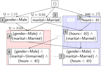
Figure 2. An overview of the lattice structure and search with support threshold $\tau=5\%$.

Toward this objective, we propose ComputeCandidates, an algorithm that takes the training data as input and generates a list of candidate patterns. Figure 2 shows an example of part of the lattice search space for patterns. ComputeCandidates generates explanations starting with patterns each having a single predicate. The algorithm then iteratively generates patterns with $i$ predicates by merging two patterns with $i-1$ predicates that differ in only one predicate. For instance, it merges patterns and in Figure 2 into pattern . The idea is similar to frequent itemset mining (10.5555/645920.672836, ; 10.1145/335191.335372, ) in data mining where itemsets with $n$ items are generated by successively merging candidate itemsets of smaller size.

By itself, building patterns bottom-up does not reduce the size of the search space. We propose two heuristics to address this issue. The first heuristic is that we assume as input a support threshold $\tau$ and only consider patterns whose support is above $\tau$. The rationale for this heuristic is that patterns with low support describe only a small portion of the training data and, thus, are unlikely to identify systematic issues. In our experiments in (techreport), with $\tau$ as small as $1\%$, we did not observe patterns with low support reducing bias by much, and found much larger patterns (with $\sim 27\%$ support) dominating the top-k. For a candidate pattern $\phi$ generated by merging patterns $\phi_{i}$ and $\phi_{j}$ we have $\sup(\phi)\leq\sup(\phi_{i})$ and $\sup(\phi)\leq\sup(\phi_{j})$. Thus, pruning $\phi_{i}$ prunes the entire sub-lattice whose root is $\phi_{i}$. In Figure 2, pattern is pruned since its support ($1\%$) is less than the threshold ($5\%$). As a result, patterns formed by merging pattern with another pattern, including patterns and and the entire sub-tree shaded blue , are also pruned.

Our second heuristic is to prune patterns during merging. Consider a pattern $\phi$ generated by merging patterns $\phi_{i}$ and $\phi_{j}$. We only consider $\phi$ if its responsibility exceeds the responsibility of the two patterns it is generated from: $\mathcal{R}(\phi)>\mathcal{R}(\phi_{i})$ and $\mathcal{R}(\phi)>\mathcal{R}(\phi_{j})$. Note that if this is the case, then $U(\phi)>\max(U(\phi_{i}),U(\phi_{j}))$, because $U(\phi)=\frac{\mathcal{R}_{\mathcal{F}}({\mathbf{D}}({\phi}))}{Sup(\phi)}$ and as mentioned above $Sup(\phi)\leq\min(Sup(\phi_{i}),Sup(\phi_{j}))$. In Figure 2, we do not generate (and subsequently its successors, shaded red ) because $U($pattern $)$ is less than both $U($pattern $)$ and $U($pattern $)$. The rationale for this heuristic is that patterns with more predicates are harder to interpret. Thus, an increase in the number of predicates should be justified by an increased impact on the bias of the model.

We now discuss our algorithm in more detail (pseudocode is shown in Algorithm 1). We start by generating all possible single predicate patterns (Algorithm 1) by iterating through all features $X\in{\mathbf{X}}$ and each possible value $val$ for the feature and generate three types of comparisons: $X<val$, $X=val$, and $X>val$. Note that for features with a large number of possible values, we can apply binning techniques to reduce the number of candidate patterns. Additionally, binning has the advantage of preventing the generation of almost identical explanations (e.g., $\texttt{{hours}}<40$ and $\texttt{{hours}}<42$).

We then iteratively create patterns (Algorithm 1) of size $i$ by merging two patterns of size $i-1$ that differ in only one predicate to generate a candidate pattern of size $i$. The algorithm terminates if no new candidates have been produced in the current iteration. For each generated candidate pattern $\phi$ we test if its support is larger than the threshold $\tau$ and its responsibility is larger than that of the patterns it was derived from. If both the conditions are fulfilled then we include $\phi$ in $\Phi_{i}$, the set of candidate patterns of size $i$. Finally, we return all candidate explanations, which is the union of all sets $\Phi_{i}$ generated so far.

Note that while merging patterns, we do not have to consider patterns that are conflicting. Patterns $\phi_{i}$ and $\phi_{j}$ are conflicting if they both contain a predicate on an attribute $X$ and the conjunction of these predicates is unsatisfiable. In Figure 2, patterns and are conflicting. The merged pattern $\phi=$ $\cup$ has zero support, and we do not need to consider it further.

Input: Training data ${\mathbf{D}}$, support threshold $\tau$

Output: Candidate explanations

1

2$\Phi_{1}\leftarrow\emptyset$ $\triangleright$ Initialize set of one-predicate explanations

3for $X\in{\mathbf{X}}$ do

4       for $val\in\pi_{X}({\mathbf{D}})$ do

5             for $\phi\in\{\{X=val\},\{X<val\},\{X>val\}\}$ do

6                   if $Sup(\phi)>\tau$ then

7                         $\Phi_{1}\leftarrow\Phi_{1}\cup\{\phi\}$

8                  

9            

10      

11

12$i\leftarrow 2$

13while $\Phi_{i-1}\neq\emptyset$ do

14       $\Phi_{i}\leftarrow\emptyset$

15      for $\phi_{i},\phi_{j}\in\Phi_{i-1}$ do

16             if $|\phi_{i}\cap\phi_{j}|=i-2\land Sup(\phi_{i}\cup\phi_{j})\geq\tau$ then

17                   $\phi=\phi_{i}\cup\phi_{j}$

18                  if $\mathcal{I}(\phi)>\mathcal{I}(\phi_{i})\land\mathcal{I}(\phi)>\mathcal{I}(\phi_{j})$ then

19                        

20                        $\Phi_{i}\leftarrow\Phi_{i}\cup\{\phi\}$

21                  

22            

23      $i\leftarrow i+1$

24

25return $\bigcup_{j=0}^{i}\Phi_{i}$

Algorithm 1 ComputeCandidates

Diversity of explanations. We use Algorithm 2 to compute a diverse set of top-k explanations as defined in Definition 3.7. We first use ComputeCandidates to generate a set of candidate explanations, which is then sorted based on the interestingness score $U$. We iterate over the set in sort order, include patterns into the result, and skip patterns whose overlap with any of the previously added patterns exceeds the threshold $c$.

We are interested in patterns that, when removed or modified, reduce bias maximally without significantly affecting model accuracy. Instead of directly optimizing for minimal accuracy loss, we penalize patterns with high support (or, low interestingness score). As an extreme example, we can remove the entire data (that has the maximum support) and obtain a perfectly unbiased classifier that makes random guesses. However, such a pattern has no explanatory value. This intuition aligns with the notion of minimality in database repair that seeks to find minimal subsets of data responsible for an inconsistency. Optimizing for bias reduction and accuracy loss simultaneously is an interesting direction for future work.

Note that Gopher’s explanations describe training data subsets that may have potential data quality errors or point to historical biases reflected in training data or bias that was introduced during data collection. These errors are not detectable using standard data cleaning algorithms such as outlier detection. Gopher can be complemented with existing error detection mechanisms or external sources of information on data provenance to expose the errors in the identified subsets.

Input: Training dataset ${\mathbf{D}}$, support threshold $\tau$, containment threshold $c$, desired number of top explanations $k$

Output: Top-k explanations

1

2$\Phi_{cand}\leftarrow\textsc{ComputeCandidates}({\mathbf{D}},\tau)$

3$\Phi_{top-k}\leftarrow\emptyset$ $\triangleright$ Set of top-k explanations

4for $\phi\in$ sort-by-score($\Phi_{cand}$) do

5       if $\neg\,\exists\phi_{j}\in\Phi_{top-k}\mathrel{\mathop{\ordinarycolon}}C(\phi,\phi_{j})>c$ then

6             $\Phi_{top-k}\leftarrow\Phi_{top-k}\cup\phi_{j}$

7      if $|\Phi_{top-k}|=k$ then

8             return $\Phi_{top-k}$

9      

10

Algorithm 2 Generate Top-k Explanations

5. Update-Based Explanations

In this section, we formalize the problem of generating explanations based on updating training data. Given an influential subset of training data obtained through the techniques proposed in Section 4, our goal is to find a homogenous update that can lead to maximum bias reduction. Toward that goal, we first discuss an approach for approximating the influence of updating or perturbing a subset of training data on model bias.

Consider a classifier with optimal parameters $\theta^{*}$ trained on a training dataset ${\mathbf{D}}$. Let ${\mathbf{S}}=\{{\mathbf{z}}_{i}=({\mathbf{X}}_{i},Y_{i})\}_{i=1}^{m}$ be a subset of ${\mathbf{D}}$ consisting of $m$ data points. Also, let ${\mathbf{S}}^{p}=\{{\mathbf{z}}_{i}^{p}=({\mathbf{X}}_{i}^{p},Y_{i}^{p})\}_{i=1}^{m}$ be the result of uniformly updating each instance in ${\mathbf{S}}$ using a perturbation vector $\boldsymbol{\delta}=\{\delta_{1},\ldots,\delta_{|{\mathbf{X}}|}\}$. The attribute values of each data point ${\mathbf{z}}\in{\mathbf{S}}$ are updated by applying the perturbation vector: ${\mathbf{z}}^{p}={\mathbf{z}}+\boldsymbol{\delta}$, i.e., the $j$-th attribute of ${\mathbf{z}}$ is updated by $\delta_{j}$. For example, if the value of the working hours attribute for an individual is $32$, then an update of $8$ will change it to $40$. In this example, uniform perturbation means that the working hours for all individuals from the subset ${\mathbf{S}}$ are increased by $8$. Our goal is to compute the optimal parameters $\theta_{p}$ for a new model trained on ${\mathbf{D}}^{p}=({\mathbf{D}}\setminus{\mathbf{S}})\ \cup\ {\mathbf{S}}^{p}$. We approximate $\theta_{p}$ using a single step of gradient descent (Section 4.1.2), as follows:

(14) $$\theta_{p}=\theta^{*}-\dfrac{\eta}{n}\left(\sum_{i=1}^{n-m}\nabla_{\theta}L({\mathbf{z}}_{i},\theta^{*})+\sum_{i=1}^{m}\nabla_{\theta}L({\mathbf{z}}_{i}^{p},\theta^{*})\right)$$

where $\eta$ is the learning rate for the gradient step.

Therefore, the influence of an update to ${\mathbf{S}}$ on the bias of the model can be measured using the chain rule, as follows:

(15) $$\Delta\mathcal{F}(\theta^{*},\theta_{p},{\mathbf{D}}_{test})=\nabla_{\theta}\mathcal{F}(\theta^{*},{\mathbf{D}}_{test})^{\top}\left(\theta_{p}-\theta^{*}\right)$$

Now, given a subset of training data, ${\mathbf{S}}\subseteq{\mathbf{D}}$, our goal is to obtain an update on ${\mathbf{S}}$ that leads to the maximum bias reduction. That is, we want to solve the following optimization problem:

(16) $$\boldsymbol{\delta}^{*}=\arg\!\max_{\boldsymbol{\delta}}\Delta\mathcal{F}(\theta^{*},\theta_{p},{\mathbf{D}}_{test})$$

Using Equations (14) and (15), Equation (16) becomes:

(17) $$\boldsymbol{\delta}^{*}=\arg\!\min_{\boldsymbol{\delta}}\nabla_{\theta}\mathcal{F}(\theta^{*},{\mathbf{D}}_{test})^{\top}\nabla_{\theta}\mathcal{L}({\mathbf{S}}^{p},\theta^{*})$$

We solve Equation (17) using the gradient descent algorithm to obtain the perturbation vector:

(18) $$\boldsymbol{\delta}_{k+1}=\boldsymbol{\delta}_{k}-\eta\nabla_{\theta}\mathcal{F}({\mathbf{D}}_{test},\theta^{*})^{\top}\nabla_{\delta}\left(\nabla_{\theta}\mathcal{L}({\mathbf{S}}^{p}+\boldsymbol{\delta}_{k},\theta^{*})\right)$$

where $\eta$ is the learning rate of the gradient ascent step.

An updated data point is obtained as ${\mathbf{z}}^{p}={\mathbf{z}}+\boldsymbol{\delta}_{k+1}$. Note that the preceding formulation can result in perturbations that lie outside the input domain. We add domain constraints to prevent this from happening. In particular, the updates should change an attribute of a data point from one value to another in the input domain, i.e., ${\mathbf{z}},{\mathbf{z}}^{p}\in\textsc{Dom}({\mathbf{X}})\times\textsc{Dom}(Y)$. We solve this constrained optimization problem in Equation 18 using projected gradient descent (intro-optimization, ), which works as follows: if the updated data point violates the domain constraint, i.e., ${\mathbf{z}}^{p}\notin\textsc{Dom}({\mathbf{X}})\times\textsc{Dom}(Y)$, then project it back to the input domain $\textsc{Dom}({\mathbf{X}})\times\textsc{Dom}(Y)$ as:

(19) $${\mathbf{z}}_{up}=\operatorname*{argmin}\limits_{{\mathbf{z}}^{\prime}\in\textsc{Dom}({\mathbf{X}})\times\textsc{Dom}(Y)}\left\lVert{\mathbf{z}}^{\prime}-{\mathbf{z}}^{p}\right\rVert$$

The projection ensures that ${\mathbf{z}}_{up}$ is the data point in the input domain $\textsc{Dom}({\mathbf{X}})\times\textsc{Dom}(Y)$ that is closest to the actual perturbation ${\mathbf{z}}^{p}$.

6. Experiments

In our experimental evaluation of Gopher, we aim to address the following questions: Q1: How effective are the proposed techniques for approximating causal responsibility of training data subsets? Q2: What is the end-to-end performance of Gopher in generating interpretable and diverse data-based explanations? Q3: What is the quality of the update-based explanations? Q4: How effective is our approach at detecting data errors responsible for ML model bias?

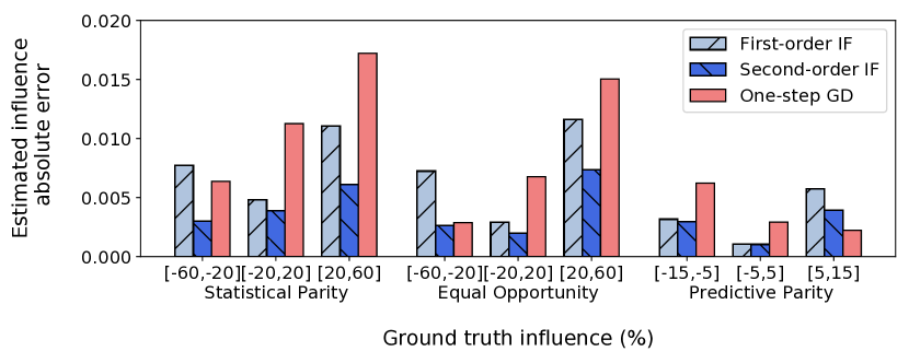
(a) Logistic regression

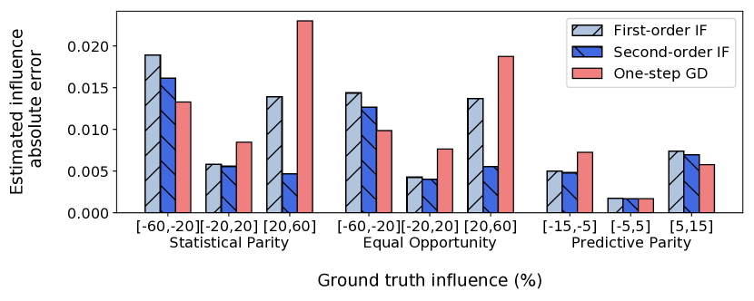
(b) Neural networks (NNs).

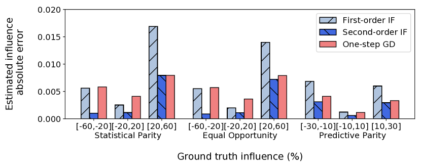
(c) Support vector machine (SVM).

Figure 3. Comparing influence function approximations (first-order IF and second-order IF) against the one-step gradient descent approach (one-step GD) for estimating subset influence on the German dataset.

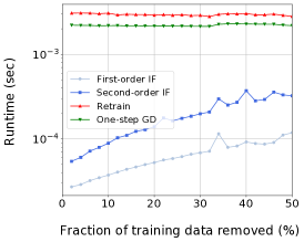
(a) Logistic regression.

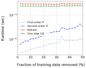
(b) Support vector machine.

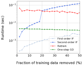
(c) Neural network.

Figure 4. Runtime (averaged over 30 runs) for computing influence for subsets of German. Influence function approximations are significantly faster than retraining and one-step gradient descent influence for smaller subsets.

6.1. Datasets

We use standard datasets from the fairness literature. The data and code for the experiments can be found at the project page.

German Credit Data (German) (Dua2019, ). Personal, financial and demographic information ($20$ attributes) of $1,000$ bank account holders. The prediction task classifies individuals as good/bad credit risks. Adult Income Data (Adult) (Dua2019, ). Demographic information, level of education, occupation, working hours, etc., of $48,000$ individuals ($14$ attributes). The task predicts whether the annual income of an individual exceeds $\$50$K. Stop, Question, and Frisk Data (SQF) (sqf-data, ). Demographic and stop-related information for $72,548$ individuals stopped and questioned (and possibly frisked) by the NYC Police Department (NYPD). The classification task is to predict if a stopped individual will be frisked.

6.2. Setup

We considered three ML algorithms: logistic regression, support vector machines, and a feed-forward neural network with 1 layer and 10 nodes (we provide details about the hyper-parameters for in the Gopher repository). We used the PyTorch (pytorch, ) or sklearn (sklearn, ) implementation of these algorithms. In accordance with existing literature on evaluation of fairness of ML algorithms on these datasets (chiappa2019path, ), the sensitive attributes are: gender (Adult), age (German), race (SQF). We implemented our algorithms in Python and used PyTorch’s autograd package to compute the gradients and Hessian. At start up, we pre-computed the Hessian and gradients for faster computation of the influence function approximations. We split each dataset into training and test data, trained an ML model over the training data, and generated explanations using our pattern generation algorithm. We report the top-k explanations for each dataset under different scenarios. For each explanation, we report the pattern $\phi$, its support $Sup(\phi)$, and the ground truth change in bias (reported in terms of statistical parity unless stated otherwise) achieved by removing the data corresponding to the pattern from the training data. We solve Equation 19 using SciPy’s optimize package for constrained optimization. For update-based explanations, we report the update to the data corresponding to the explanation’s pattern and the change in bias resulting from the update. For both kinds of explanations, predicates that occur in more than one pattern are color-coded. We use the logistic regression model as the default ML model.

Baseline. As a competitor for our approach, we trained a decision tree regressor (referred to as FO-tree) over FO influence approximations of data points. FO-tree splits the training data into non-overlapping subsets based on the values of an attribute at a node of the tree. The path from the root to a node of the tree corresponds to a conjunction of predicates that characterize the data points represented by that node. To generate the top-$k$ explanations consisting of up to $l$ predicates, we identify the $k$ nodes from the root (level 0) to level $l$ that have the maximum combined influence of data points, and report the paths from the root node to these nodes. For example, to generate top-5 explanations with up to 3 predicates, we identify the 5 nodes up to a depth of 3 having the maximum FO influence and report the conjunction of predicates that form the path from the root to each of these node.

6.3. Causal Responsibility Approximations

In this set of experiments, we evaluated the quality of the proposed approaches for approximating influence, and thereby causal responsibility. The ground truth influence of subsets is computed by retraining the model after removing the subset from the training data. To estimate subset influence using FO approximations, we summed the individual influences, whereas the SO subset influence is computed using Equation 10. We also compared the approximations for the one-step gradient descent approach described in Section 4.1.2, because we use this approach for update explanations.

Pattern	Support	$\Delta_{bias}$
	$5.00\%$	$55.2\%$
	$6.25\%$	$35.8\%$
	$5.13\%$	$14.8\%$

Table 1. Top-$3$ explanations for German ($\tau=5\%$, logistic regression, runtime=$18$s).

Pattern	Support	$\Delta_{bias}$
	$7.89\%$	$12.00\%$
	$6.27\%$	$11.01\%$
	$7.39\%$	$6.02\%$

Table 2. Top-$3$ explanations on Adult ($\tau=5\%$, neural networks, runtime=$56$s).

Pattern	Support	$\Delta_{bias}$
	$16.89\%$	$25.6\%$
	$12.95\%$	$13.7\%$
	$7.04\%$	$8.16\%$

Table 3. Top-$3$ explanations for SQF ($\tau=5\%$, logistic regression, runtime=$91$s).

Effectiveness. In Figures 3(a), 3(b) and 3(c), we report the absolute deviation of the influence estimated by the different methods from the ground truth (y-axis) for the fairness definitions (x-axis) described in Section 2. We trained different classifiers on the German dataset. We observed that, as expected, FO influence approximations and one-step gradient descent deviated more from ground truth influence than SO influence. FO influence approximation exhibits larger errors because it does not account for possible correlations among data points in the subset (basu2020second, ); one-step gradient descent influence approximation is not accurate because it uses a single step of gradient descent instead of iterating until the model parameters converge. This behavior is especially evident when the size of the group is large, which usually corresponds to large influence (the bars on the outside of a metric). The key takeaway from this experiment is that SO influence functions closely approximate ground truth influence especially when model parameters do not change substantially (the middle bars).

Efficiency. In Figure 4, we report the average time taken by each method when subsets of varying sizes are removed from the training data. The brute force approach – retraining the model after removing the subset – is typically more than two orders of magnitude slower than even the most expensive method, especially when the fraction of removed training data points is small (e.g., influence functions are up to $4$ orders of magnitude faster when 0%-10% of the training dataset is deleted). We also observe that the one-step gradient descent approach, with the exception for SO influence functions on neural networks, while effective in estimating ground truth influence (as shown in Figure 3(a), Figure 3(c)), is significantly slower than influence functions for estimating subset influence. Note that the time cost for retraining is close to that of one-step gradient descent because we used the initial model parameters to speed up convergence during retraining. In practice, we have to adjust the learning rate for one-step gradient descent over multiple iterations, which makes it even more expensive. We conclude that retraining the model and using the one-step gradient descent approach are not feasible for generating the top-$k$ explanations. The one-step gradient descent, however, is useful for generating update-based explanations as described in Section 4.1.2: influence functions are not applicable to the optimization problem we have to solve for updates, and retraining is also not an option.

6.4. End-to-end Performance

Next, we evaluate the performance of Gopher for generating the top-$k$ explanations for ML algorithms trained on different datasets.

German. This dataset is biased toward older individuals and considers them less likely to be characterized as high credit risks. In Table 1, we report the top-$3$ explanations up to 4 predicates generated by Gopher (with their support and ground truth influence) sorted by their interestingness score. We observe that one subset of $5\%$ of data points explains more than half of the model bias, whereas another subset of around $6\%$ of data points reduces bias by almost $36\%$. These explanations highlight fractions of training data that may have potential errors and hence, need attention. On inspection, we found that they correspond to training data points where older individuals are primarily labeled as low credit risks. By removing these individuals, the probability of an individual being classified as a high/low credit risk is uniformly distributed across the sensitive attribute age. As a result, the model’s dependency on age is reduced, thus reducing overall model bias. Note that the top-2 explanations consist of predicates with the sensitive attribute for this dataset, signifying its importance in bias reduction. In comparison, we made the following observations about the explanations generated by FO-tree: entirely different regressor trees, and hence different explanations, were generated depending upon whether sklearn or PyTorch was used to fit the model. While the sensitive attribute (age) formed the root node for the FO-tree generated on the PyTorch model, a non-intuitive attribute (installment rate) was the root in the FO-tree for the sklearn model. The top-2 explanations from FO-tree over the PyTorch model were consistent with our explanations whereas those generated from FO-tree over the sklearn model were less compact (consisting of 4 predicates each). Their (support, bias reduction) were ($6.13\%,32.3\%$), ($5.63\%,33.1\%$) and ($12.9\%,8\%$), respectively.

Pattern	Support	$\Delta_{bias}$
	$5\%$	$55.2\%$
		$42.0\%\downarrow$
	$6.25\%$	$35.8\%$
		$21.6\%\downarrow$
	$5.13\%$	$14.8\%$
		$5.4\%\downarrow$

Table 4. Update-based explanations for the top-3 explanations for German ( $\tau=5\%$). Updates to the original explanation (top) are shown with a bold outline (bottom). Change in bias reduction due to the update $\Delta_{bias}$ is represented by $\downarrow$ (decrease) or $\uparrow$ (increase). Average time taken to update each point = $0.22$s.

Pattern	Support	$\Delta_{bias}$
	$9.1\%$	$13.3\%$
		$13.8\%\uparrow$
	$14.3\%$	$19.1\%$
		$0.6\%\downarrow$
	$7.6\%$	$9.1\%$
		$9.5\%\uparrow$

Table 5. Update-based explanations for the top-3 explanations for Adult ( $\tau=5\%$). Updates to the original explanation (top) are shown in bold outline (bottom). Change in bias reduction $\Delta_{bias}$ is represented by $\downarrow$ (decrease) or $\uparrow$ (increase). Average time taken to update each point = $0.24$s.

Pattern	Support	$\Delta_{bias}$
	$16.9\%$	$25.6\%$
		$14.3\%\downarrow$
	$13.0\%$	$13.7\%$
		$8.6\%\downarrow$
	$7.0\%$	$8.2\%$
		$13.7\%\uparrow$

Table 6. Update-based explanations for the top-3 explanations for SQF ( $\tau=5\%$). Updates to the original explanation (top) are shown in bold outline (bottom). Change in bias reduction $\Delta_{bias}$ is represented by $\downarrow$ (decrease) or $\uparrow$ (increase). Average time taken to update each point = $0.5$s

Adult. This dataset has been at the center of several studies that analyze the impact of gender (TAGH+17, ; DBLP:conf/sigmod/SalimiGS18, ) and has been shown to be inconsistent: income attributes for married individuals report household income. The dataset has more married males, indicating a favorable bias toward males. As seen in Table 2, the sensitive attribute gender plays an important role in all of the explanations. In this set of experiments on neural networks, we observed that second-order influence functions did not estimate the model parameters accurately and greatly underestimated the ground truth influence. This observation was consistent with the analysis provided in (basu2020second, ) for neural networks where the influence of a group of data points has low correlation with ground truth influence, and second-order influences underestimate ground truth influence. Our approach hinges on the applicability of influence functions to correctly estimate the model parameters around the optimal parameters– an assumption that might not hold for neural networks. Gopher still identified patterns that reduce model bias to some extent. In comparison, the top-3 patterns returned by FO-tree had higher support and lower ground truth influence: ($10.9\%,9.8\%$), ($13.2\%,10.8\%$) and ($5.9\%,11\%$), respectively. Note that even though the dataset has single predicates ([marital = Married], $\sim 47\%$ data) that remove bias almost completely, these predicates do not rank in the top-$k$ explanations because of their low interestingness scores.

SQF. This dataset highlighted that the practices of NYPD in stopping, questioning and frisking blacks (and latinos) more often compared to whites were unconstitutional and violated Fourth Amendment rights (sqf-nyclu, ). In Table 3, our top-3 explanations identify patterns consisting of the protected group that were frisked and the privileged group that were not frisked. Because of these data points, the model learns that data points belonging to the privileged (protected) group are less (more) likely to be frisked, and therefore, cause bias in the model. By removing these data points, the privileged group becomes less correlated with the ‘no frisk’ outcome, thus reducing model bias. The topmost explanation generated by the FO-tree [(location=Outside) $\wedge$ (race=White) $\wedge$ (build¡¿Thin) $\wedge$ (does not fit a relevant description)] had similar support ($13.2\%$) and bias reduction ($27\%$) as our topmost explanation. The other two patterns had lower bias reduction (one of them had $0.15\%$ reduction in bias) and greater support, and hence were less interesting.

6.5. Update-based Explanations

In these experiments, we generated updates for the top-$k$ explanations. For each explanation, we provide the perturbation that would result in the maximum bias reduction.

German. As seen in Table 4, updates typically involve perturbing the protected attribute (age). For example, the first explanation suggests that by updating data points satisfying the pattern such that after the update they are in the protected instead of the privileged group, and by changing the gender to increase the chance of a positive outcome, bias is reduced by $42\%$. In this case, we found an update that would reduce model bias but not by as much as deleting those points would. Similarly, in explanation 2, older individuals that have a good credit history are considered low credit risks. By changing their age group to the protected group and credit history to a worse level, we now associate younger individuals with good credit risk and reduce model bias (albeit by an amount smaller than if the group was removed). The key takeaway here is that we can reduce model bias by updating the training data points referring to these patterns instead of removing them altogether.

Adult. We report the update-based explanations for this dataset in Table 5. As mentioned before, this subset is biased toward married individuals and males. In explanation 1, individuals that were not married had lower income. By changing their marital status to married, we were able to reduce model bias by at least as much as would have been achieved were those patterns deleted. Note, however, that in explanation 2, even by changing the gender and marital status to the preferred attribute values, we could not find an appropriate update that would reduce the bias. After marital status, we found that education accounts for most of the bias (DBLP:conf/sigmod/SalimiGS18, )– individuals with a higher level of education are associated with higher incomes. In explanation 2, by changing the education level we were able to reduce bias by almost the same amount as would have been achieved if the subset were altogether removed.

SQF. In Table 6, we observe that changing particular attribute values can help us avoid discriminatory behavior for this dataset. For example, before the update in explanation 3, whites that appeared to be casing a victim (or studying them for probable targets) were not frisked — a clear case of discrimination. In this case, we were able to find an update such that they did not case a victim even when close to the crime scene, and achieved even more reduction in model bias than if this subpopulation is removed altogether. Similarly, frisking blacks even when they do not fit a relevant description was biased against them. In this case, updating this subset of data points such that whites that fit a relevant description are frisked reduced the model bias but less than if the subset is removed.

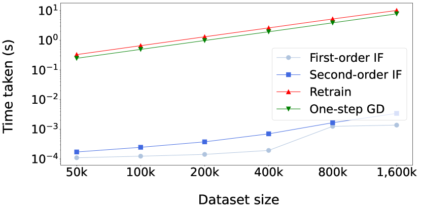
Figure 5. Runtime vs. dataset size.

6.6. Scalability Analysis

To evaluate the scalability of influence computations, we report in Figure 5 the effect of dataset size on the time taken to compute influence of a subset by the approaches described in Section 4.1. We replicated German to increase its size by a factor of $50$ to $1,600$ yielding up to 1.6M training data points. To evaluate how dataset sizes affect influence computation runtimes, we fixed the size of the subset for which we compute the subset influence to $5\%$ (this threshold reflects our problem setting where we are interested in small fractions of training data that need attention). We observed that both FO and SO influence computations scale well in the dataset size, and achieve speed-ups of several orders of magnitude over retraining the model or using one-step gradient descent. Note that Gopher has an upfront cost of pre-computing the gradients of the loss function and the Hessian. Once these computations are done, the time taken to compute subset influence is negligible (as seen in Figure 5). In contrast, model retraining to compute subset influence can be quite expensive. For example, using the feed-forward network on Adult, we observed that the pre-computations took $\sim 1,800s$ and the top-$3$ explanations were generated in $56s$ for a total time cost of $\sim 1,856s$. In comparison, retraining the model after removing one subset took $>10s$. We see benefit in using Gopher when a relatively large number of candidates are being considered to generate top-k explanations (which is the case with our datasets).

In Table 7, we report the time taken to generate the top-$5$ explanations on German when we allow more predicates in an explanation (indicated by the level in the lattice structure), and hence consider greater number of candidates. We observe that Gopher’s explanation generation using the lattice structure has good scalability (runtimes of $<25$ min) for explanations with fewer predicates. In comparison, our filtering mechanism that accounts for diversity of explanations takes negligible amount of time (although considering more candidates increases the runtime of the filtering step).

Level	1	2	3	4	5	6
execution (s)	0.03	0.24	1.59	17.5	269	1,472
filtering (ms)	36	45	70	75	76	90
#candidates	29	371	2,770	13,625	36,704	62,955

Table 7. Scalability in the number of candidate patterns.

6.7. Detecting data errors

To test the viability of Gopher in detecting data errors, we applied our implementation as a detection mechanism for errors injected by data poisoning attacks  (mehrabi-bias, ; koh-data-poisoning, ). The objective was to develop techniques to detect attacks that have superior performance (measured in terms of accuracy and fairness) on training data and are targeted at exacerbating model performance on test data. The state of the art in safeguarding against data poisoning attacks is to detect anomalies that do not conform to the rest of the data. However, anomaly detection fails in the presence of sophisticated attacks that are targeted at deteriorating model accuracy and/or fairness (solans2020poisoning, ; jagielski2020subpopulation, ; mehrabi2020exacerbating, ; goel2021importance, ). We performed experiments where we injected poisoned data points into the training data using non-random anchoring attacks (mehrabi-bias, ). We found that the outlier detection mechanism supported by scikit-learn (sklearn, ), LocalOutlierFactor, was not able to detect any of the poisoned data points, because they follow a similar distribution as the original training data points. In comparison, when the data was clustered (using k-means or Gaussian mixture models clustering) and clusters were ranked in decreasing order of estimated SO influence, we observed that the top-2 clusters contained almost $70\%$ of poisoned points. While these results are promising, a detailed study demonstrating the effectiveness of second-order influence functions in detecting adversarial attacks is out of the scope of this work and is an interesting direction for future work.

7. Related Work

Our work relates to the following lines of research.

Feature-based explanations. Much of XAI research focuses on explaining ML models in terms of dependencies between input features and their outcomes. Feature attribution methods quantify the responsibility of input features for model predictions (vstrumbelj2014explaining, ; lundberg2017unified, ; datta2016algorithmic, ; merrick2019explanation, ; frye2019asymmetric, ; aas2019explaining, ). Methods based on surrogate explainability approximate ML models using a simple, interpretable model  (lundberg2017unified, ; ribeiro2016should, ). Contrastive and causal methods explain ML model predictions in terms of minimal interventions or perturbations on input features that change the prediction (verma2020counterfactual, ; wachter2017counterfactual, ; karimi2019model, ; ustun2019actionable, ; mahajan2019preserving, ; mothilal2020explaining, ; DBLP:conf/sigmod/BertossiLSSV20, ; galhotra2021explaining, ). Logic-based methods operate on logical representations of ML algorithms (shih2018symbolic, ; ignatiev2020towards, ; darwiche2020reasons, ) to compute minimal sets of features that are sufficient and necessary for ML model predictions. These approaches fall short in generating diagnostic explanations that help users trace an ML model’s unexpected or discriminatory behavior back to its training data.

Explanations based on training data. In contrast, data-based explanations attribute ML model predictions to specific parts of training data (AREA-202009-Brophy, ). A popular approach ranks individual training data points based on their influence on model predictions (koh2017understanding, ; basu2020second, ) using influence functions (cook-influence, )— a classic technique from robust statistics that measure how optimal model parameters depend on training data points. Based on first-order influence functions, Rain (Wu2020ComplaintdrivenTD, ) identifies data points responsible for user constraints specified by an SQL query. Several recent works argue for the use of data Shapley values to quantify the contribution of individual data points (pmlr-v130-kwon21a, ; pmlr-v119-ghorbani20a, ; DBLP:conf/icml/GhorbaniZ19, ), which is computationally expensive because the model needs to be retrained for each data point. Representer points explain the predictions of neural networks by decomposing the pre-activation prediction into a linear combination of activations of training points (yeh2018representer, ). PrIU (Wu2020PrIUAP, ) is a provenance-based approach that incrementally computes the effect of removing a subset of training data points. Unlike prior methods, we generate: (1) explanations for the bias of an ML model, (2) interpretable explanations based on first-order predicates that pinpoint a training data subset responsible for model bias, and (3) update-based explanations that reveal data errors in certain attributes of a training data subset. It is worth mentioning that model bias can be reduced not only by removing subsets of training data but also by adding appropriate training samples. Searching for in-distribution data points that explain away bias upon insertion into training data is a challenging problem that we plan to explore in the future. Note that our update-based explanations act as a combination of removing existing data points and adding new ones.

Debugging ML models. Several recent works address debugging of ML models for bias, including fair-DAGs (Yang2020FairnessAwareIO, ) and mlinspect (10.1145/3448016.3452759, ) that attribute discrimination to class imbalance and address bias by tracking the distribution of sensitive attributes along ML pipelines. A closely related idea identifies regions of the input domain that are not adequately covered by training data (asudeh2021identifying, ; asudeh2019assessing, ). MLDebugger (10.1145/3329486.3329489, ) identifies minimal causes of unsatisfactory performance in ML pipelines using provenance of the previous runs. These approaches cannot highlight parts of training data responsible for biased outputs. DUTI (zhang2018training, ) identifies the smallest set of changes to training data labels so the model trained on the updated data can correctly predict labels of a trusted set of items from test data; this approach focuses on updating training labels, and is not applicable to our setting. Another line of work finds data slices in which the model performs poorly  (8713886, ; 47966, ; 10.1145/3448016.3457323, ); slices are discovered based on their association with model error and do not capture the causal effect of interventions. These techniques are not directly applicable to fairness where, unlike model error, bias due to a subset is not additive. Moreover, none of these interventions update data instances.

Adversarial ML. We share similarities with adversarial ML that aims to degrade ML model fairness or predictions through adversarial attacks. The most relevant classes of attacks are based on data poisoning (steinhardt2017certified, ; chen2017targeted, ), which injects a minimum set of synthetic data points into the training data to compromise the performance or fairness of a model trained on the contaminated data (solans2020poisoning, ; jagielski2020subpopulation, ; mehrabi2020exacerbating, ). In contrast, our goal is to detect those points.

Machine unlearning. Our research also relates to the nascent field of machine unlearning (bourtoule2019machine, ; gupta2021adaptive, ; schelter2021hedgecut, ; izzo2021approximate, ), which addresses the “right to be forgotten” provisioned in recent legislations, such as the General Data Protection Regulation (GDPR) in the European Union (voigt2017eu, ) and the California Consumer Privacy Act in the United States (de2018guide, ). Current methods are typically designed for particular classes of ML models e.g., HedgeCut (schelter2021hedgecut, ) supports efficient unlearning requests for decision trees. The techniques in this sub-field could be integrated into our framework for efficient computation of causal responsibility. We defer this investigation to future study.

Bias detection and mitigation. Prior work to detect and mitigate bias in ML models can be categorized into pre-, post- and in-processing methods (Caton2020FairnessIM, ). We aim to pre-process data to reduce bias by removing bias and discrimination signals from training data (NIPS2017_6988, ; feldman2015certifying, ; salimi2019interventional, ), which is different from post-processing that deals with model output to handle bias, and in-processing that is aimed at building fair ML models. Pre-processing methods are independent of the downstream ML model, are usually not interpretable, and hence are insufficient in generating explanations that reveal the potential source of bias. While not a direct focus of our research, our approach could help develop bias mitigation algorithms that are interpretable and account for the downstream ML model; hence, they would incur minimal information loss and generalize better. We defer this research to future work.

8. Conclusions

We present a novel approach for debugging bias in machine learning models by identifying coherent subsets of training data that are responsible for the bias. We introduce Gopher, a principled framework for reasoning about the responsibility of such subsets and develop an efficient algorithm that produces explanations, which compactly describe responsible sets of training data points through patterns. We demonstrate experimentally that Gopher is efficient and produces explanations that are interpretable and correctly identify sources of bias for datasets where ground truth biases are well understood. In the future, we plan to expand our approach beyond supervised ML algorithms with differentiable loss functions to support a wider range of ML algorithms such as tree-based ML models and clustering algorithms. Moreover, we plan to leverage database techniques for incremental maintenance to efficiently compute causal responsibility as opposed to approximating it. Another interesting future direction is to integrate Gopher with database provenance to formalize the notion of provenance of ML model decisions that trace ML model outcomes all the way back to decisions made in the ML pipeline that might explain the bias and unexpected behavior of the model.

References

- [1] NYPD stop, question and frisk data. https://www1.nyc.gov/site/nypd/stats/reports-analysis/stopfrisk.page. [Online; accessed 19-October-2021].
- [2] Stop-and-frisk in the de blasio era. https://www.nyclu.org/en/publications/stop-and-frisk-de-blasio-era-2019. [Online; accessed 19-October-2021].
- [3] Housing department slaps facebook with discrimination charge. https://www.npr.org/2019/03/28/707614254/hud-slaps-facebook-with-housing-discrimination-charge, 2019.
- [4] Self-driving cars more likely to hit blacks. https://www.technologyreview.com/2019/03/01/136808/self-driving-cars-are-coming-but-accidents-may-not-be-evenly-distributed/, 2019.
- [5] Kjersti Aas, Martin Jullum, and Anders Løland. Explaining individual predictions when features are dependent: More accurate approximations to shapley values. arXiv preprint arXiv:1903.10464, 2019.
- [6] Rakesh Agrawal and Ramakrishnan Srikant. Fast algorithms for mining association rules in large databases. In Proceedings of the 20th International Conference on Very Large Data Bases, VLDB ’94, page 487–499, San Francisco, CA, USA, 1994. Morgan Kaufmann Publishers Inc.
- [7] Abolfazl Asudeh, Zhongjun Jin, and HV Jagadish. Assessing and remedying coverage for a given dataset. In 2019 IEEE 35th International Conference on Data Engineering (ICDE), pages 554–565. IEEE, 2019.
- [8] Abolfazl Asudeh, Nima Shahbazi, Zhongjun Jin, and HV Jagadish. Identifying insufficient data coverage for ordinal continuous-valued attributes. In Proceedings of the 2021 International Conference on Management of Data, pages 129–141, 2021.
- [9] Samyadeep Basu, Xuchen You, and Soheil Feizi. On second-order group influence functions for black-box predictions. In Proceedings of Machine Learning and Systems 2020, pages 7503–7512. 2020.
- [10] Samyadeep Basu, Xuchen You, and Soheil Feizi. On second-order group influence functions for black-box predictions. In International Conference on Machine Learning, pages 715–724. PMLR, 2020.
- [11] Leopoldo E. Bertossi, Jordan Li, Maximilian Schleich, Dan Suciu, and Zografoula Vagena. Causality-based explanation of classification outcomes. In Proceedings of the Fourth Workshop on Data Management for End-To-End Machine Learning, In conjunction with the 2020 ACM SIGMOD/PODS Conference, DEEM@SIGMOD 2020, Portland, OR, USA, June 14, 2020, pages 6:1–6:10, 2020.
- [12] Reuben Binns, Max Van Kleek, Michael Veale, Ulrik Lyngs, Jun Zhao, and Nigel Shadbolt. ’it’s reducing a human being to a percentage’ perceptions of justice in algorithmic decisions. In Proceedings of the 2018 Chi conference on human factors in computing systems, pages 1–14, 2018.
- [13] Lucas Bourtoule, Varun Chandrasekaran, Christopher A Choquette-Choo, Hengrui Jia, Adelin Travers, Baiwu Zhang, David Lie, and Nicolas Papernot. Machine unlearning. arXiv preprint arXiv:1912.03817, 2019.
- [14] Jonathan Brophy. Exit through the training data: A look into instance-attribution explanations and efficient data deletion in machine learning. Area exam, University of Oregon, Computer and Information Sciences Department, 9 2020. Available at https://www.cs.uoregon.edu/Reports/AREA-202009-Brophy.pdf.
- [15] Sébastien Bubeck. Convex optimization: Algorithms and complexity. Found. Trends Mach. Learn., 8:231–357, 2015.
- [16] Flavio Calmon, Dennis Wei, Bhanukiran Vinzamuri, Karthikeyan Natesan Ramamurthy, and Kush R Varshney. Optimized pre-processing for discrimination prevention. In I. Guyon, U. V. Luxburg, S. Bengio, H. Wallach, R. Fergus, S. Vishwanathan, and R. Garnett, editors, Advances in Neural Information Processing Systems 30, pages 3992–4001. Curran Associates, Inc., 2017.
- [17] Simon Caton and C. Haas. Fairness in machine learning: A survey. ArXiv, abs/2010.04053, 2020.
- [18] Xinyun Chen, Chang Liu, Bo Li, Kimberly Lu, and Dawn Song. Targeted backdoor attacks on deep learning systems using data poisoning. arXiv preprint arXiv:1712.05526, 2017.
- [19] Silvia Chiappa. Path-specific counterfactual fairness. In Proceedings of the AAAI Conference on Artificial Intelligence, volume 33, pages 7801–7808, 2019.
- [20] Edwin Kah Pin Chong and Stanislaw H. Zak. An introduction to optimization. John Wiley & Sons, 2013.
- [21] Y. Chung, T. Kraska, N. Polyzotis, K. Tae, and S. Whang. Automated data slicing for model validation: A big data - ai integration approach. IEEE Transactions on Knowledge & Data Engineering, 32(12):2284–2296, dec 2020.
- [22] Dennis R. Cook and Sanford Weisberg. Characterizations of an empirical influence function for detecting influential cases in regression. Technometrics, 22, 1980.
- [23] Adnan Darwiche and Auguste Hirth. On the reasons behind decisions. arXiv preprint arXiv:2002.09284, 2020.
- [24] Anupam Datta, Shayak Sen, and Yair Zick. Algorithmic transparency via quantitative input influence: Theory and experiments with learning systems. In 2016 IEEE symposium on security and privacy (SP), pages 598–617. IEEE, 2016.
- [25] Lydia de la Torre. A guide to the california consumer privacy act of 2018. Available at SSRN 3275571, 2018.
- [26] Dheeru Dua and Casey Graff. UCI machine learning repository, 2017.
- [27] Tom Farrand, Fatemehsadat Mireshghallah, Sahib Singh, and Andrew Trask. Neither private nor fair: Impact of data imbalance on utility and fairness in differential privacy. In Proceedings of the 2020 Workshop on Privacy-Preserving Machine Learning in Practice, pages 15–19, 2020.
- [28] Michael Feldman, Sorelle A. Friedler, John Moeller, Carlos Scheidegger, and Suresh Venkatasubramanian. Certifying and removing disparate impact. In KDD, pages 259–268. ACM, 2015.
- [29] Martínez-Plumed Fernando, Ferri Cèsar, Nieves David, and Hernández-Orallo José. Missing the missing values: The ugly duckling of fairness in machine learning. International Journal of Intelligent Systems, 2021.
- [30] Christopher Frye, Ilya Feige, and Colin Rowat. Asymmetric shapley values: incorporating causal knowledge into model-agnostic explainability. arXiv preprint arXiv:1910.06358, 2019.
- [31] Runshan Fu, Yan Huang, and P. Singh. Ai and algorithmic bias: Source, detection, mitigation and implications. Social Science Research Network, 2020.
- [32] Sainyam Galhotra, Romila Pradhan, and Babak Salimi. Explaining black-box algorithms using probabilistic contrastive counterfactuals. In Proceedings of the 2021 International Conference on Management of Data, pages 577–590, 2021.
- [33] Amirata Ghorbani, Michael Kim, and James Zou. A distributional framework for data valuation. In Hal Daumé III and Aarti Singh, editors, Proceedings of the 37th International Conference on Machine Learning, volume 119 of Proceedings of Machine Learning Research, pages 3535–3544. PMLR, 13–18 Jul 2020.
- [34] Amirata Ghorbani and James Y. Zou. Data shapley: Equitable valuation of data for machine learning. In Kamalika Chaudhuri and Ruslan Salakhutdinov, editors, Proceedings of the 36th International Conference on Machine Learning, ICML 2019, 9-15 June 2019, Long Beach, California, USA, volume 97 of Proceedings of Machine Learning Research, pages 2242–2251. PMLR, 2019.
- [35] Milena A Gianfrancesco, Suzanne Tamang, Jinoos Yazdany, and Gabriela Schmajuk. Potential biases in machine learning algorithms using electronic health record data. JAMA internal medicine, 178(11):1544–1547, 2018.
- [36] Naman Goel, Alfonso Amayuelas, Amit Deshpande, and Amit Sharma. The importance of modeling data missingness in algorithmic fairness: A causal perspective. In Proceedings of the AAAI Conference on Artificial Intelligence, volume 35, pages 7564–7573, 2021.
- [37] Stefan Grafberger, Shubha Guha, Julia Stoyanovich, and Sebastian Schelter. Mlinspect: A data distribution debugger for machine learning pipelines. In Proceedings of the 2021 International Conference on Management of Data, SIGMOD/PODS ’21, page 2736–2739, New York, NY, USA, 2021. Association for Computing Machinery.
- [38] Varun Gupta, Christopher Jung, Seth Neel, Aaron Roth, Saeed Sharifi-Malvajerdi, and Chris Waites. Adaptive machine unlearning. arXiv preprint arXiv:2106.04378, 2021.
- [39] Jiawei Han, Jian Pei, and Yiwen Yin. Mining frequent patterns without candidate generation. SIGMOD Rec., 29(2):1–12, May 2000.
- [40] Alexey Ignatiev. Towards trustable explainable ai. In 29th International Joint Conference on Artificial Intelligence, pages 5154–5158, 2020.
- [41] Zachary Izzo, Mary Anne Smart, Kamalika Chaudhuri, and James Zou. Approximate data deletion from machine learning models. In International Conference on Artificial Intelligence and Statistics, pages 2008–2016. PMLR, 2021.
- [42] Abigail Z Jacobs and Hanna Wallach. Measurement and fairness. In Proceedings of the 2021 ACM Conference on Fairness, Accountability, and Transparency, pages 375–385, 2021.
- [43] Matthew Jagielski, Giorgio Severi, Niklas Pousette Harger, and Alina Oprea. Subpopulation data poisoning attacks. arXiv preprint arXiv:2006.14026, 2020.
- [44] Matthew Jagielski, Giorgio Severi, Niklas Pousette Harger, and Alina Oprea. Subpopulation data poisoning attacks. CoRR, abs/2006.14026, 2020.
- [45] Amir-Hossein Karimi, Gilles Barthe, Borja Belle, and Isabel Valera. Model-agnostic counterfactual explanations for consequential decisions. arXiv preprint arXiv:1905.11190, 2019.
- [46] Atoosa Kasirzadeh. Reasons, values, stakeholders: A philosophical framework for explainable artificial intelligence. In Proceedings of the 2021 ACM Conference on Fairness, Accountability, and Transparency, pages 14–14, 2021.
- [47] Matthew Kay, Cynthia Matuszek, and Sean A. Munson. Unequal representation and gender stereotypes in image search results for occupations. In Proceedings of the 33rd Annual ACM Conference on Human Factors in Computing Systems, CHI ’15, page 3819–3828, New York, NY, USA, 2015. Association for Computing Machinery.
- [48] Jakko Kemper and Daan Kolkman. Transparent to whom? no algorithmic accountability without a critical audience. Information, Communication & Society, 22(14):2081–2096, 2019.
- [49] Niki Kilbertus, Mateo Rojas Carulla, Giambattista Parascandolo, Moritz Hardt, Dominik Janzing, and Bernhard Schölkopf. Avoiding discrimination through causal reasoning. In Advances in Neural Information Processing Systems, pages 656–666, 2017.
- [50] Pang Wei Koh and Percy Liang. Understanding black-box predictions via influence functions. volume 70 of Proceedings of Machine Learning Research, pages 1885–1894, International Convention Centre, Sydney, Australia, 06–11 Aug 2017. PMLR.
- [51] Pang Wei Koh and Percy Liang. Understanding black-box predictions via influence functions. In International Conference on Machine Learning, pages 1885–1894. PMLR, 2017.
- [52] Pang Wei Koh, Jacob Steinhardt, and Percy Liang. Stronger data poisoning attacks break data sanitization defenses. arXiv 2018.
- [53] Matt J Kusner, Joshua Loftus, Chris Russell, and Ricardo Silva. Counterfactual fairness. In Advances in Neural Information Processing Systems, pages 4069–4079, 2017.
- [54] Yongchan Kwon, Manuel A. Rivas, and James Zou. Efficient computation and analysis of distributional shapley values. In Arindam Banerjee and Kenji Fukumizu, editors, Proceedings of The 24th International Conference on Artificial Intelligence and Statistics, volume 130 of Proceedings of Machine Learning Research, pages 793–801. PMLR, 13–15 Apr 2021.
- [55] Thibault Laugel, Marie-Jeanne Lesot, Christophe Marsala, Xavier Renard, and Marcin Detyniecki. Inverse classification for comparison-based interpretability in machine learning. arXiv preprint arXiv:1712.08443, 2017.
- [56] Bruno Lepri, Nuria Oliver, Emmanuel Letouzé, Alex Pentland, and Patrick Vinck. Fair, transparent, and accountable algorithmic decision-making processes. Philosophy & Technology, 31(4):611–627, 2018.
- [57] Stan Lipovetsky and Michael Conklin. Analysis of regression in game theory approach. Applied Stochastic Models in Business and Industry, 17(4):319–330, 2001.
- [58] Raoni Lourenço, Juliana Freire, and Dennis Shasha. Debugging machine learning pipelines. In Proceedings of the 3rd International Workshop on Data Management for End-to-End Machine Learning, DEEM’19, New York, NY, USA, 2019. Association for Computing Machinery.
- [59] Scott M Lundberg, Gabriel G Erion, and Su-In Lee. Consistent individualized feature attribution for tree ensembles. arXiv preprint arXiv:1802.03888, 2018.
- [60] Scott M Lundberg and Su-In Lee. A unified approach to interpreting model predictions. In Advances in neural information processing systems, pages 4765–4774, 2017.
- [61] Divyat Mahajan, Chenhao Tan, and Amit Sharma. Preserving causal constraints in counterfactual explanations for machine learning classifiers. arXiv preprint arXiv:1912.03277, 2019.
- [62] Fernando Martínez-Plumed, Cèsar Ferri, David Nieves, and José Hernández-Orallo. Fairness and missing values. arXiv preprint arXiv:1905.12728, 2019.
- [63] Ninareh Mehrabi, Fred Morstatter, Nripsuta Saxena, Kristina Lerman, and Aram Galstyan. A survey on bias and fairness in machine learning. arXiv preprint arXiv:1908.09635, 2019.
- [64] Ninareh Mehrabi, Muhammad Naveed, Fred Morstatter, and Aram Galstyan. Exacerbating algorithmic bias through fairness attacks. To appear in Proceedings of AAAI 2021.
- [65] Ninareh Mehrabi, Muhammad Naveed, Fred Morstatter, and Aram Galstyan. Exacerbating algorithmic bias through fairness attacks. arXiv preprint arXiv:2012.08723, 2020.
- [66] Luke Merrick and Ankur Taly. The explanation game: Explaining machine learning models with cooperative game theory. arXiv preprint arXiv:1909.08128, 2019.
- [67] Christoph Molnar. Interpretable Machine Learning. Lulu. com, 2020.
- [68] Ramaravind K Mothilal, Amit Sharma, and Chenhao Tan. Explaining machine learning classifiers through diverse counterfactual explanations. In Proceedings of the 2020 Conference on Fairness, Accountability, and Transparency, pages 607–617, 2020.
- [69] Razieh Nabi and Ilya Shpitser. Fair inference on outcomes. In Proceedings of the… AAAI Conference on Artificial Intelligence. AAAI Conference on Artificial Intelligence, volume 2018, page 1931. NIH Public Access, 2018.
- [70] Ravi B Parikh, Stephanie Teeple, and Amol S Navathe. Addressing bias in artificial intelligence in health care. Jama, 322(24):2377–2378, 2019.
- [71] Adam Paszke, Sam Gross, Francisco Massa, Adam Lerer, James Bradbury, Gregory Chanan, Trevor Killeen, Zeming Lin, Natalia Gimelshein, Luca Antiga, Alban Desmaison, Andreas Kopf, Edward Yang, Zachary DeVito, Martin Raison, Alykhan Tejani, Sasank Chilamkurthy, Benoit Steiner, Lu Fang, Junjie Bai, and Soumith Chintala. Pytorch: An imperative style, high-performance deep learning library. In H. Wallach, H. Larochelle, A. Beygelzimer, F. d'Alché-Buc, E. Fox, and R. Garnett, editors, Advances in Neural Information Processing Systems 32, pages 8024–8035. Curran Associates, Inc., 2019.
- [72] F. Pedregosa, G. Varoquaux, A. Gramfort, V. Michel, B. Thirion, O. Grisel, M. Blondel, P. Prettenhofer, R. Weiss, V. Dubourg, J. Vanderplas, A. Passos, D. Cournapeau, M. Brucher, M. Perrot, and E. Duchesnay. Scikit-learn: Machine learning in Python. Journal of Machine Learning Research, 12:2825–2830, 2011.
- [73] Neoklis Polyzotis, Steven Whang, Tim Klas Kraska, and Yeounoh Chung. Slice finder: Automated data slicing for model validation. In Proceedings of the IEEE Int’ Conf. on Data Engineering (ICDE), 2019, 2019.
- [74] Ashkan Rezaei, Anqi Liu, Omid Memarrast, and Brian Ziebart. Robust fairness under covariate shift. arXiv preprint arXiv:2010.05166, 2020.
- [75] Marco Tulio Ribeiro, Sameer Singh, and Carlos Guestrin. ” why should i trust you?” explaining the predictions of any classifier. In Proceedings of the 22nd ACM SIGKDD international conference on knowledge discovery and data mining, pages 1135–1144, 2016.
- [76] Marco Tulio Ribeiro, Sameer Singh, and Carlos Guestrin. Anchors: High-precision model-agnostic explanations. In AAAI, volume 18, pages 1527–1535, 2018.
- [77] Svetlana Sagadeeva and Matthias Boehm. Sliceline: Fast, linear-algebra-based slice finding for ml model debugging. In Proceedings of the 2021 International Conference on Management of Data, SIGMOD/PODS ’21, page 2290–2299, New York, NY, USA, 2021. Association for Computing Machinery.
- [78] Babak Salimi, Johannes Gehrke, and Dan Suciu. Bias in OLAP queries: Detection, explanation, and removal. In Proceedings of the 2018 International Conference on Management of Data, SIGMOD Conference 2018, Houston, TX, USA, June 10-15, 2018, pages 1021–1035, 2018.
- [79] Babak Salimi, Luke Rodriguez, Bill Howe, and Dan Suciu. Interventional fairness: Causal database repair for algorithmic fairness. In Proceedings of the 2019 International Conference on Management of Data, pages 793–810. ACM, 2019.
- [80] Sebastian Schelter, Stefan Grafberger, and Ted Dunning. Hedgecut: Maintaining randomised trees for low-latency machine unlearning. In Proceedings of the 2021 International Conference on Management of Data, pages 1545–1557, 2021.
- [81] Andy Shih, Arthur Choi, and Adnan Darwiche. A symbolic approach to explaining bayesian network classifiers. arXiv preprint arXiv:1805.03364, 2018.
- [82] Harvineet Singh, Rina Singh, Vishwali Mhasawade, and Rumi Chunara. Fairness violations and mitigation under covariate shift. In Proceedings of the 2021 ACM Conference on Fairness, Accountability, and Transparency, pages 3–13, 2021.
- [83] David Solans, Battista Biggio, and Carlos Castillo. Poisoning attacks on algorithmic fairness. arXiv preprint arXiv:2004.07401, 2020.
- [84] Jacob Steinhardt, Pang Wei Koh, and Percy Liang. Certified defenses for data poisoning attacks. In Proceedings of the 31st International Conference on Neural Information Processing Systems, pages 3520–3532, 2017.
- [85] Julia Stoyanovich, Bill Howe, and H. V. Jagadish. Responsible data management. Proceedings of the VLDB Endowment, 13:3474 – 3488, 2020.
- [86] Erik Štrumbelj and Igor Kononenko. Explaining prediction models and individual predictions with feature contributions. Knowledge and information systems, 41(3):647–665, 2014.
- [87] Florian Tramèr, Vaggelis Atlidakis, Roxana Geambasu, Daniel Hsu, Jean-Pierre Hubaux, Mathias Humbert, Ari Juels, and Huang Lin. Fairtest: Discovering unwarranted associations in data-driven applications. In IEEE European Symposium on Security and Privacy (EuroS&P). IEEE, 2017.
- [88] https://docs.fast.ai/tabular.learner.htm. Fastai neural network.
- [89] Berk Ustun, Alexander Spangher, and Yang Liu. Actionable recourse in linear classification. In Proceedings of the Conference on Fairness, Accountability, and Transparency, pages 10–19, 2019.
- [90] Sahil Verma, John Dickerson, and Keegan Hines. Counterfactual explanations for machine learning: A review. arXiv preprint arXiv:2010.10596, 2020.
- [91] Sahil Verma and Julia Rubin. Fairness definitions explained. In Proceedings of the International Workshop on Software Fairness, FairWare ’18, page 1–7, New York, NY, USA, 2018. Association for Computing Machinery.
- [92] Paul Voigt and Axel Von dem Bussche. The eu general data protection regulation (gdpr). A Practical Guide, 1st Ed., Cham: Springer International Publishing, 10:3152676, 2017.
- [93] Sandra Wachter, Brent Mittelstadt, and Chris Russell. Counterfactual explanations without opening the black box: Automated decisions and the gdpr. Harv. JL & Tech., 31:841, 2017.
- [94] Jialu Wang, Yang Liu, and Caleb Levy. Fair classification with group-dependent label noise. In Proceedings of the 2021 ACM Conference on Fairness, Accountability, and Transparency, pages 526–536, 2021.
- [95] Weiyuan Wu, Lampros Flokas, Eugene Wu, and Jiannan Wang. Complaint-driven training data debugging for query 2.0. Proceedings of the 2020 ACM SIGMOD International Conference on Management of Data, 2020.
- [96] Yinjun Wu, V. Tannen, and S. Davidson. Priu: A provenance-based approach for incrementally updating regression models. Proceedings of the 2020 ACM SIGMOD International Conference on Management of Data, 2020.
- [97] K. Yang, Biao Huang, Julia Stoyanovich, and Sebastian Schelter. Fairness-aware instrumentation of preprocessing pipelines for machine learning. 2020.
- [98] Chih-Kuan Yeh, Joon Sik Kim, Ian EH Yen, and Pradeep Ravikumar. Representer point selection for explaining deep neural networks. arXiv preprint arXiv:1811.09720, 2018.
- [99] Xuezhou Zhang, Xiaojin Zhu, and Stephen Wright. Training set debugging using trusted items. In Thirty-second AAAI conference on artificial intelligence, 2018.