Optimized integrating factor technique for Schrödinger-like equations

Abstract.

The integrating factor technique is widely used to solve numerically (in particular) the Schrödinger equation in the context of spectral methods. Here, we present an improvement of this method exploiting the freedom provided by the gauge condition of the potential. Optimal gauge conditions are derived considering the equation and the temporal numerical resolution with an adaptive embedded scheme of arbitrary order. We illustrate this approach with the nonlinear Schrödinger (NLS) and with the Schrödinger–Newton (SN) equations. We show that this optimization increases significantly the overall computational speed, sometimes by a factor five or more. This gain is crucial for long time simulations.

Key words: Gauge optimization; Schrödinger equation; time-stepping; integrating factor.

1. Introduction

The Schrödinger equation is used in many field of Physics. In dimensionless units, it takes the form

$$\mathrm{i}\,\partial_{t}\,\psi\ +\ {\textstyle{\frac{1}{2}}}\,\nabla^{2}\psi\ -\ V\,\psi\ =\ 0,$$ (1)

where $\psi$ is a function of the spatial coordinates $\boldsymbol{r}$ and of the time $t$, $\nabla^{2}$ is the Laplace operator, and the potential $V$ is generally a function of space and time and, possibly, a functional of $\psi$. In this paper, we focus more specifically on the nonlinear Schrödinger equation ($V$ proportional to $|\psi|^{2}$) and on the Schrödinger–Newton (or Schrödinger–Poisson) equation in which the Laplacian of the potential is proportional to $|\psi|^{2}$. These special cases were chosen for clarity and because they are of practical interest, but the method presented here can be extended to more general potentials (and equations).

With the nonlinear Schrödinger equation (NLS) considered here, the (local nonlinear) potential is

$$V\ =\ g\,|\psi|^{2},$$ (2)

where $g$ is a coupling constant. For $g>0$ the interaction is repulsive, while, for $g<0$ it is attractive. The NLS describes various physical phenomena, such as Bose–Einstein condensates [1], laser beams in some nonlinear media [2], water wave packets [3], etc.

With the Schrödinger–Poisson equation, the potential is given by the Poisson equation

$$\nabla^{2}\,V\ =\ g\,|\psi|^{2},$$ (3)

where $g$ is another coupling constant, the interaction being attractive if $g>0$ and repulsive if $g<0$. It is therefore nonlinear and non-local, giving rise to collective phenomena [4], appearing for instance in optics [5, 6, 7], Bose–Einstein condensates [8], cosmology [9, 10, 11] and theories describing the quantum collapse of the wave function [12, 13]. It is also used as a model to perform cosmological simulations in the semi-classical limit [14].

The above equations cannot be solved analytically (except for very special cases) and numerical methods must be employed. In this paper, we focus on spectral methods for the spatial resolution, i.e., methods that are based on fast Fourier transform (FFT) techniques, that are specially efficient and accurate [15]. For the temporal resolution, two families of methods are commonly employed to solve Schrödinger-like equations: integrating factors [16] and split-step integrators [17]. The latter methods have been used to integrate both the SN and NLS equations, but the former is used essentially to solve the NLS, with very performing results [18, 19]. In this note, we focus on the former technique, which consists in integrating analytically the linear part of the equation and integrating numerically the remaining nonlinear part with a classical method [16]. The principle of the method is described as follow.

Writing the Schrödinger equation in the generic form

$$\mathrm{i}\,\partial_{t}\,\psi\ =\ F\!\left(\boldsymbol{r},t,\psi\right),\qquad\psi\ =\ \psi\!\left(\boldsymbol{r},t\right),$$ (4)

the right-hand side is split into linear and nonlinear parts

$$\mathrm{i}\,\partial_{t}\,\psi\ +\ \mathcal{L}\,\psi\ =\ \mathcal{N}\!\left(\boldsymbol{r},t,\psi\right),$$ (5)

where $\mathcal{L}$ is an easily computable autonomous linear operator and $\mathcal{N}\stackrel{{\scriptstyle\text{\tiny{def}}}}{{=}}F+\mathcal{L}\psi$ is the remaining (usually) nonlinear part. At the $n$-th time-step, with $t\in[t_{n},t_{n+1}]$, considering the change of dependent variable

$$\phi\ \stackrel{{\scriptstyle\text{\tiny{def}}}}{{=}}\ \exp\!\left[\,(t-t_{n})\,\mathcal{L}\,\right]\psi\qquad\implies\qquad\mathrm{i}\,\partial_{t}\,\psi\ =\ \exp\!\left[\,(t_{n}-t)\,\mathcal{L}\,\right]\left(\,\mathrm{i}\,\partial_{t}\,\phi\,-\,\mathcal{L}\,\phi\,\right),$$ (6)

so $\phi=\psi$ at $t=t_{n}$, the equation (5) is rewritten

$$\mathrm{i}\,\partial_{t}\,\phi\ =\,\exp\!\left[\,(t-t_{n})\,\mathcal{L}\,\right]\mathcal{N}.$$ (7)

The operator $\mathcal{L}$ being well chosen, the stiffness of (5) is considerably reduced and the equation (7) is (hopefully) well approximated by algebraic polynomials for $t\in[t_{n};t_{n+1}]$. Thus, standard time-stepping methods, such as an adaptive Runge–Kutta method [20, 21], can be used to efficiently solve (7). To do so, the solution is evaluated at two different orders and a local error is estimated as the difference between those quantities. Popular integrators can be found in [20, 22].

It is straightforward to apply this strategy to the Schrödinger equation (1) since ${\textstyle{\frac{1}{2}}}\nabla^{2}\psi$ and the potential $V$ are, respectively, linear and nonlinear operators of $\psi$. By switching to Fourier space in position, the equation becomes

$$\mathrm{i}\,\partial_{t}\,\widehat{\psi}\ -\ {\textstyle{\frac{1}{2}}}\,k^{2}\,\widehat{\psi}\ -\ \widehat{\/V\,\psi\/}\ =\ 0,$$ (8)

where hats denote the Fourier transform of the underneath quantity and $k\stackrel{{\scriptstyle\text{\tiny{def}}}}{{=}}|\boldsymbol{k}|$ ($\boldsymbol{k}$ the wave vector). The equation is now in a form where the application of the integrating factor (IF) method is straightforward, i.e., (8) becomes

$$\mathrm{i}\,\partial_{t}\,\phi\ =\ -\/\mathrm{i}\,\exp[{\textstyle{\frac{\mathrm{i}}{2}}}\/k^{2}\/(t-t_{n})\/]\,\widehat{\/V\,\psi\/},$$ (9)

where $\phi(\boldsymbol{k},t)\stackrel{{\scriptstyle\text{\tiny{def}}}}{{=}}\widehat{\psi}(\boldsymbol{k},t)\exp[{\textstyle{\frac{\mathrm{i}}{2}}}\/k^{2}\/(t-t_{n})\/]$. If the nonlinear part of the equation is zero, then $\mathrm{i}\,\partial_{t}\,\phi=0$ and any (reasonable) temporal scheme will produce the exact solution $\phi(t)=\phi(t_{n})$. In other words, the integrating factor technique is exact for linear equations. This indicates that the numerical errors depend on the magnitude of the nonlinear part. Therefore, in order to minimise these errors, a strategy consists in minimizing the magnitude of $\mathcal{N}$ at each time-step. To do so, we exploit the gauge invariance of the Schrödinger equation: if $\psi$ is a solution of (1) at a given time $t$, then $\Psi\ \stackrel{{\scriptstyle\text{\tiny{def}}}}{{=}}\psi\,\mathrm{e}^{-\/\mathrm{i}\,\mathcal{C}\,t}$ is a solution of

$$\mathrm{i}\,\partial_{t}\,\Psi\ +\ {\textstyle{\frac{1}{2}}}\,\nabla^{2}\Psi\ -\ \left(V+\mathcal{C}\right)\,\Psi\ =\ 0,$$ (10)

as one can easily verify. Thus, at each time-step, adding a constant $\mathcal{C}_{n}$ to $V$ in (1), modifies the solution as

$$\psi(t_{n})\ \to\ \psi(t_{n})\,\mathrm{e}^{-\/\mathrm{i}\/\varphi},\qquad\varphi\ \stackrel{{\scriptstyle\text{\tiny{def}}}}{{=}}\ \sum_{j=1}^{n}\mathcal{C}_{j}\,h_{j},$$ (11)

where $h_{j}\stackrel{{\scriptstyle\text{\tiny{def}}}}{{=}}t_{j+1}-t_{j}$ is the $j$-th time-step. Of course, at the end of the computations, the operation (11) can be easily reverted if the original phase is relevant. Using this procedure, we observed up to a five-fold speed increase (the overall computational time is divided by about five) compared to taking $\mathcal{C}_{n}=0$. Of course, the speed-up varies depending on the initial condition, of the (spatial and temporal) numerical schemes and on the choice of gauge corresponding to $\mathcal{C}_{n}=0$.

In this paper, we derive some analytic formulas giving an optimal $\mathcal{C}_{n}$ in order to maximise the time-step, i.e., to minimize the overall computational time of the numerical resolution. We emphasize that the thus obtained optimal values of $\mathcal{C}_{n}$ do not affect the accuracy of the numerical solution, leaving it unchanged with respect to the $\mathcal{C}_{n}=0$ case. Two strategies are presented. In section 2, a first ‘natural’ approach to derive a suitable $\mathcal{C}_{n}$ is based on the analytical structure of the equation and it is independent of the numerical algorithm employed for its resolution. More precisely, $\mathcal{C}_{n}$ is obtained minimizing a norm of the right-hand side of the equation (5). This provides an easy manner to obtain a formula that is moreover computationally ‘cheap’. This expression is however only near optimal, so a ‘better’ expression is subsequently derived. Considering both the equations and the numerical algorithms, a second optimal expression for $\mathcal{C}_{n}$ is derived in section 3. This approach consists in minimizing exactly the numerical error and thus explicitly dependents on the numerical scheme. This provides a more accurate, but computationally expensive, solution. The advances of these special choices are illustrated numerically in section 4. Finally, a summary and perspectives are drawn in section 5.

2. Near optimal $\mathcal{C}_{n}$

As mentioned above, if properly chosen, the integrating factor is able to reduce the stiffness of the equation, making the numerical integration more efficient. In addition, the magnitude of the nonlinear part of (7) also contributes to the efficiency of the numerical integration. Specifically, if $\mathcal{N}$ is zero, $\partial_{t}\,\phi=0$ and the integrating factor technique is exact. Thus, the efficiency of the algorithm is expected to increase as the magnitude of $\mathcal{N}$ gets smaller, and subsequently the overall computational time should be reduced. Here, we show how to choose the arbitrary constant $\mathcal{C}_{n}$ in order to reduce the magnitude of the nonlinear part $\mathcal{N}$. In the case of the Schrödinger equation, we have

$$\mathcal{N}\!\left(\boldsymbol{k},t;\phi;\mathcal{C}_{n}\right)\ =\ -\/\mathrm{i}\,\exp[{\textstyle{\frac{\mathrm{i}}{2}}}\/k^{2}\/(t-t_{n})\/]\,\mathcal{F}\{\left(V+\mathcal{C}_{n}\right)\,\psi\},$$ (12)

where $\mathcal{F}$ denotes the Fourier transform and $\psi(\boldsymbol{x},t)=\mathcal{F}^{-1}\{\exp[-{\textstyle{\frac{\mathrm{i}}{2}}}\/k^{2}\/(t-t_{n})\/]\,{\phi}(\boldsymbol{k},t)\}$.

A natural strategy is to minimize the $L_{2}$-norm, namely

$$\mathcal{G}_{n}(\mathcal{C}_{n})\stackrel{{\scriptstyle\text{\tiny{def}}}}{{=}}\frac{1}{M}\,\sum_{m=-\left[M/2\right]}^{\left[M/2\right]-1}|\,\mathcal{N}\!\left(\boldsymbol{k}_{m},t_{n};\phi;\mathcal{C}_{n}\right)|^{2},$$ (13)

where $M$ is the number of spatial modes, square brackets denote the integer part and $\boldsymbol{k}_{m}$ is the $m$-th Fourier mode. The explicit expression of $\mathcal{G}_{n}$ can be found exploiting the definition of the discrete Fourier transform. For simplicity, we do the calculations in one dimension (1D) without loss of generality, since the final result is independent of the spatial dimension $d$. From Parseval theorem, one obtains

$$\mathcal{G}_{n}(\mathcal{C}_{n})\ =\sum_{\ell=-\left[M/2\right]}^{\left[M/2\right]-1}(V_{\ell}+\mathcal{C}_{n})^{2}\,|\psi_{\ell}|^{2},$$ (14)

where $\psi_{\ell}\stackrel{{\scriptstyle\text{\tiny{def}}}}{{=}}\psi({\boldsymbol{x}}_{\ell})$ and $V_{\ell}\stackrel{{\scriptstyle\text{\tiny{def}}}}{{=}}V({\boldsymbol{x}}_{\ell})$ at time $t_{n}$. Since the function $\mathcal{G}_{n}(\mathcal{C}_{n})$ is a second-order polynomial in $\mathcal{C}_{n}$, it admits an unique minimum, which is obtained from the equation $\mathrm{d}G_{n}(\mathcal{C}_{n})/\mathrm{d}\mathcal{C}_{n}=0$, yielding

$$\mathcal{C}_{n}\,=\,-\left(\,\sum_{\ell=-\left[M/2\right]}^{\left[M/2\right]-1}V_{\ell}\,\left|\psi_{\ell}\right|^{2}\,\right)\,\left/\,\left(\,\sum_{\ell=-\left[M/2\right]}^{\left[M/2\right]-1}\left|\psi_{\ell}\right|^{2}\,\right)\right.\stackrel{{\scriptstyle\text{\tiny{def}}}}{{=}}\,\tilde{\mathcal{C}}_{n}.$$ (15)

Therefore, at each time step $n$, $\tilde{\mathcal{C}}_{n}$, which is the value of $\mathcal{C}_{n}$ minimizing the $L_{2}$-norm of $\mathcal{N}$, is obtained from (15). We show below that even though this approach is not unique (i.e., different norms could be considered), the provided solution is quite advantageous compared to others, being computationally cheap and independent on the order of the numerical scheme.

3. Optimal $\mathcal{C}_{n}$

We show here another way to choose the arbitrary constant $\mathcal{C}_{n}$ in order to improve the algorithm efficiency and reduce the overall computational time. This approach is based on the principles of the adaptive time-step procedure, where at each time step $n$, an error $\Delta_{n}$ between two approximated solutions of different orders is estimated. Since the smaller this quantity the larger the time-step, minimizing $\Delta_{n}$ allows to choose a larger time-step, speeding-up the numerical integration and keeping roughly the same numerical error. More specifically, the error $\Delta_{n}$ depends on the arbitrary constant $\mathcal{C}_{n}$, hence the minimization can be performed (see below) choosing an appropriate $\mathcal{C}_{n}$. In this section, we first recall the method for determining the size of the time step used in the Runge–Kutta procedures; interested readers should refer to [20] for further details. Although the determination of $\mathcal{C}_{n}$ can be formally presented for any embedded Runge–Kutta schemes, this results in very cumbersome calculations with little insights. Thus, for brevity and clarity, we illustrate the method with the Heun method (that is a second-order Runge–Kutta method with an embedded first-order explicit Euler scheme for the time stepping [23]). We then sketch-out how this procedure can be implemented for generic embedded Runge–Kutta methods.

3.1. Principle of the adaptive time-step procedure

For the time stepping, embedded Runge–Kutta methods estimate the quadrature error comparing the results of two orders of the time integrator [20]. For a solver of order $N$ with an embedded $(N-1)$-order scheme (hereafter schemes of orders $\{N,N-1\}$), at the $n$-th time step, the error $\Delta_{n}$ is [24]

$$\Delta_{n}\ \stackrel{{\scriptstyle\text{\tiny{def}}}}{{=}}\ \sqrt{\frac{1}{M}\sum_{m=-\left[M/2\right]}^{\left[M/2\right]-1}\left(\frac{\left|\,\phi(\boldsymbol{k}_{m},t_{n})\,-\,\widetilde{\phi}(\boldsymbol{k}_{m},t_{n})\,\right|}{\mbox{\sc Tol}\,+\,\max\!\left(\left|\phi(\boldsymbol{k}_{m},t_{n})\right|,\left|\tilde{\phi}(\boldsymbol{k}_{m},t_{n})\right|\right)\times\mbox{\sc Tol}}\right)^{2}},$$ (16)

where $M$ is the number of spatial modes, square brackets denote the integer part, $\phi(\boldsymbol{k}_{m},t_{n})$ is the $N$-th order solution at the $m$-th Fourier mode, the tilde notation indicating the solution at order $N-1$, and Tol is the tolerance (parameter defining the desired precision of the time-integration). The time step $h_{n}$ is accepted if the error $\Delta_{n}$ is smaller than the tolerance Tol, otherwise $h_{n}$ is reduced and this step is recomputed. $h_{n}$ being accepted, the next time step $h_{n+1}$ is obtained assuming the largest error equal to the tolerance. In order to avoid an excess of rejected time steps, we use the Proportional Integral (PI) Step Control [24], which chooses the optimal time step $h_{n+1}$ as

$$h_{n+1}\ =\ h_{n}\,\Delta_{n}^{\,-b}\,\Delta_{n-1}^{\,c},$$ (17)

where $b=0.7/p$, $c=0.4/p$, $p$ being the order of the chosen integrator [25]. Interested readers should refer to [20] for details on this classical procedure.

3.2. Optimum time step

Since the constant $\mathcal{C}_{n}$ can be chosen freely, we seek for the value of $\mathcal{C}_{n}$ providing the largest $h_{n+1}$, namely, to maximize the right-hand side of (17). Since $h_{n}$ and $\Delta_{n-1}$ are determined at the previous time-step, only $\Delta_{n}$ in (17) depends on $\mathcal{C}_{n}$. Thus, in order to maximize $h_{n+1}$, $\Delta_{n}$ must be minimized, i.e., one must solve $\mathrm{d}\Delta_{n}/\mathrm{d}\mathcal{C}_{n}=0$. This derivation being characterized by cumbersome algebra for general embedded Runge–Kutta schemes, we illustrate the case of the Heun algorithm (that is a second-order Runge–Kutta method with an embedded first-order explicit Euler scheme for the time stepping [23]), the principle being the same for higher order integrators. Also for simplicity, we give the calculations in one dimension (1D) without loss of generality, since the final result is independent of the spatial dimension.

3.2.1. Optimum $\mathcal{C}_{n}$ for Heun’s method

Heun’s method consists, here, in solving the initial value problem (for $t\geqslant t_{n}$)

$$\mathrm{i}\,\partial_{t}\,\phi\ =\ f({\boldsymbol{k}},t;\phi;\mathcal{C}_{n})\,\stackrel{{\scriptstyle\text{\tiny{def}}}}{{=}}\,-\/\mathrm{i}\,\exp\!\left[\,{\textstyle{\frac{\mathrm{i}}{2}}}\,k^{2}\,(t-t_{n})\,\right]\mathcal{F}\{\,(V+\mathcal{C}_{n})\,\psi\,\},$$ (18)

and

$$\phi({\boldsymbol{k}},t)\, \stackrel{{\scriptstyle\text{\tiny{def}}}}{{=}}\,\exp\!\left[\,{\textstyle{\frac{\mathrm{i}}{2}}}\,k^{2}\,(t-t_{n})\,\right]\mathcal{F}\{\psi({\boldsymbol{x}},t)\}.$$ (19)

Hereafter, for brevity, we denote

$$\phi_{n}\,=\,\phi_{n}({\boldsymbol{k}})\ \stackrel{{\scriptstyle\text{\tiny{def}}}}{{=}}\ \phi({\boldsymbol{k}},t_{n}),\qquad\psi_{n}\,=\,\psi_{n}({\boldsymbol{x}})\stackrel{{\scriptstyle\text{\tiny{def}}}}{{=}}\ \psi({\boldsymbol{x}},t_{n}),\qquad V_{n}\,=\,V_{n}({\boldsymbol{x}})\stackrel{{\scriptstyle\text{\tiny{def}}}}{{=}}V({\boldsymbol{x}},t_{n}).$$ (20)

At time $t=t_{n+1}$, the first- and second-order (in $h_{n}$) approximations of $\phi$, respectively $\widetilde{\phi}_{n+1}$ and $\phi_{n+1}$, are

$$\widetilde{\phi}_{n+1}\ =\ \phi_{n}\ +\ h_{n}\,f({\boldsymbol{k}},t_{n};\phi_{n};\mathcal{C}_{n}),$$ (21)

$$\phi_{n+1}\ =\ \phi_{n}\ +\ {\textstyle{\frac{1}{2}}}\,h_{n}\left[\,f({\boldsymbol{k}},t_{n};\phi_{n};\mathcal{C}_{n})\,+\,f\!\left({\boldsymbol{k}},t_{n}+h_{n};\phi_{n}+h_{n}\/f({\boldsymbol{k}},t_{n};\phi_{n};\mathcal{C}_{n});\mathcal{C}_{n}\right)\,\right].$$ (22)

The next time-step $h_{n+1}$ is chosen using equation (17). For our equation, the difference between the first- and second-order approximations $\Delta\phi_{n+1}\stackrel{{\scriptstyle\text{\tiny{def}}}}{{=}}\left|\phi_{n+1}-\widetilde{\phi}_{n+1}\right|$ is such that

$$\left(\Delta\phi_{n+1}\right)^{2}\ =\ {\textstyle{1\over 4}}\,h_{n}^{\,2}\left|\,f({\boldsymbol{k}},t_{n};\phi_{n};\mathcal{C}_{n})\,-\,f\!\left({\boldsymbol{k}},t_{n}+h_{n};\phi_{n}+h_{n}\/f({\boldsymbol{k}},t_{n};\phi_{n};\mathcal{C}_{n});\mathcal{C}_{n}\right)\,\right|^{2}$$

$$=\ {\textstyle{1\over 4}}\,h_{n}^{\,2}\left|f({\boldsymbol{k}},t_{n};\phi_{n};\mathcal{C}_{n})\,+\,\mathrm{i}\,\mathrm{e}^{\mathrm{i}\/k^{2}\/h_{n}/2}\times\right.$$

$$\qquad\qquad\left.\mathcal{F}\left\{(V_{n+1}+\mathcal{C}_{n})\/\mathcal{F}^{-1}\left\{\mathrm{e}^{-\mathrm{i}\/k^{2}\/h_{n}/2}\left(\phi_{n}+h_{n}f({\boldsymbol{k}},t_{n};\phi_{n};\mathcal{C}_{n})\right)\right\}\right\}\/\right|^{2},$$ (23)

where $V_{n+1}=V({\boldsymbol{x}},t_{n}+h_{n})$. We note that the absolute value in (3.2.1) is of first-order in $h_{n}$, as one can easily check with a Taylor expansion around $h_{n}=0$, so $\left(\Delta\phi_{n+1}\right)^{2}=O\!\left(h_{n}^{\,4}\right)$. More precisely, after some elementary algebra, one finds

$$\left(\Delta\phi_{n+1}\right)^{2}\ =\ {\textstyle{1\over 4}}\,h_{n}^{\,4}\,\,\left|\mathcal{F}\left\{(V_{n}+\mathcal{C}_{n})^{2}\,\psi_{n}\right\}\ +\ \mathrm{i}\,\mathcal{F}\left\{\partial_{t}V_{n}\,\psi_{n}\right\}\ +\ \mathcal{F}\left\{\partial_{x}V_{n}\,\partial_{x}\psi_{n}\right\}\right.$$ (24)

$$\left.+\ {\textstyle{\frac{1}{2}}}\,\mathcal{F}\left\{\partial_{xx}V_{n}\,\psi_{n}\right\}\ \right|^{2}\ +\ O\!\left(h_{n}^{\,5}\right),$$

which, defining

$$\alpha({\boldsymbol{x}},t;\mathcal{C}_{n})\, \stackrel{{\scriptstyle\text{\tiny{def}}}}{{=}}\,(V_{n}+\mathcal{C}_{n})^{2}\,\psi_{n},\qquad\beta({\boldsymbol{x}},t)\,\stackrel{{\scriptstyle\text{\tiny{def}}}}{{=}}\,\mathrm{i}\,\partial_{t}V_{n}\,\psi_{n}\ +\ \partial_{x}V_{n}\,\partial_{x}\psi_{n}+\ {\textstyle{\frac{1}{2}}}\,\partial_{xx}V_{n}\,\psi_{n},$$ (25)

can be rewritten as

$$\left(\Delta\phi_{n+1}\right)^{2}\ =\ {\textstyle{1\over 4}}\,h_{n}^{\,4}\,\,\left|\mathcal{F}\left\{\alpha(\mathcal{C}_{n})+\beta\right\}\right|^{2}\ +\ O\!\left(h_{n}^{\,5}\right).$$ (26)

Introducing the mean quadratic error

$$E_{n}(\mathcal{C}_{n})\,\stackrel{{\scriptstyle\text{\tiny{def}}}}{{=}}\ \frac{1}{M}\,\sum_{m=-\left[M/2\right]}^{\left[M/2\right]-1}\Delta\phi_{n+1}^{2}(\boldsymbol{k}_{m},t_{n};\mathcal{C}_{n}),$$ (27)

substituting (26) into (27) and exploiting the definition of the discrete Fourier transform, one obtains (using Parseval theorem)

$$E_{n}(\mathcal{C}_{n})\ =\frac{1}{M}\,\sum_{m=-\left[M/2\right]}^{\left[M/2\right]-1}\left|\sum_{\ell=-\left[M/2\right]}^{\left[M/2\right]-1}\mathrm{e}^{-\/2\/\mathrm{i}\/\pi\/m\/\ell/M}(\alpha_{\ell}(\mathcal{C}_{n})+\beta_{\ell})\,\right|^{2}\,{\textstyle{1\over 4}}\,h_{n}^{\,4}\ +\ O\!\left(h_{n}^{\,5}\right)$$

$$=\sum_{\ell=-\left[M/2\right]}^{\left[M/2\right]-1}\left|\alpha_{\ell}(\mathcal{C}_{n})+\beta_{\ell}\right|^{2}\,{\textstyle{1\over 4}}\,h_{n}^{\,4}\,+\ O\!\left(h_{n}^{\,5}\right).$$ (28)

The minimum of $E_{n}(\mathcal{C}_{n})$, obtained from the equation $\mathrm{d}E_{n}(\mathcal{C}_{n})/\mathrm{d}\mathcal{C}_{n}=0$, is such that

$$\sum_{\ell=-\left[M/2\right]}^{\left[M/2\right]-1}\frac{\mathrm{d}\left|\alpha_{\ell}(\mathcal{C}_{n})\right|^{2}}{\mathrm{d}\mathcal{C}_{n}}\ +\ 2\,\operatorname{Re}\left(\frac{\mathrm{d}\alpha_{\ell}(\mathcal{C}_{n})}{\mathrm{d}\mathcal{C}_{n}}\beta^{*}_{\ell}\right)\,=\,0,$$ (29)

Therefore, the optimum $\hat{\mathcal{C}}_{n}$ providing the largest $h_{n+1}$, in the case of Heun’s method, is a solution of (29).

3.2.2. Optimum $\mathcal{C}_{n}$ for generic embedded Runge–Kutta schemes

The optimum $\mathcal{C}_{n}$ for general embedded Runge–Kutta schemes can be obtained following the same principles illustrated above with the Heun algorithm. However, the algebraic calculations get rapidly very cumbersome, leading to expensive computations that, in most cases, exceeds the time gained with a larger step. Here, we sketch-out the procedure for generic embedded Runge–Kutta methods, considering solvers of order $N$ with an embedded $(N-1)$-order scheme (for other embedded or extrapolation methods, the procedure is completely analogue). For a $s$-stage method, the error $\Delta\phi_{n+1}$ can be written as [24]

$$\left(\Delta\phi_{n+1}\right)^{2}\,=\,\left|\sum_{\ell=1}^{s}d_{\ell}\,w_{\ell}\right|^{2},\quad d_{\ell}\stackrel{{\scriptstyle\text{\tiny{def}}}}{{=}}a_{s,\ell}-b_{\ell},\quad w_{\ell}\stackrel{{\scriptstyle\text{\tiny{def}}}}{{=}}\,h_{n}\,f\left({\boldsymbol{k}},t_{n}+c_{\ell}\,h_{n};\phi_{n}+\sum_{r=1}^{\ell-1}a_{\ell,r}\,w_{r};\mathcal{C}_{n}\right),$$ (30)

where $a_{\ell,r}$, $b_{\ell}$ and $c_{\ell}$ are the coefficients of the Butcher tableau which characterizes the integrator [24]. Using Taylor expansions and un-nesting the scheme, it is possible to prove that a result with a similar structure compared with (26) is obtained. In this case, the number of stages $s$ appears as exponent in the function $\alpha$, which takes the form $\alpha({\boldsymbol{x}},t;\mathcal{C}_{n})=(V_{n}+\mathcal{C}_{n})^{2s}\,\psi_{n}$. The function $\beta$, on the other hand, becomes explicitly dependent on $\mathcal{C}_{n}$, involving a number of terms growing exponentially with $s$. For this reason, even though the exact result can always be achieved, the computational time needed to minimize the error (16) is often larger than the time gained with a larger step, especially for higher order schemes ($s>3$). In the next section, we show how, for practical applications, an exact solution is not necessary to improve the algorithm, and (15) represents a fast and accurate method.

4. Numerical examples

Here, we consider numerical examples where we apply this method, focusing on both the SN and NLS equations solved with the Dormand and Prince 5(4) integrator [22] in one and two spatial dimensions. In all cases, we set open boundary conditions for the potential, while the initial conditions and the value of the physical parameters are chosen to be very close to regimes of physical interest, as described in [1, 2, 3]. Details on the numerical simulations can be found in A. The gain factor provided by the method depends on the optimal value of $\mathcal{C}_{n}$ compared to the $\mathcal{C}_{n}=0$ case, which changes from case to case as a function of the boundary conditions for the potential and of the profile of the solution. Specifically, since the gain factor is evaluated with respect to the $\mathcal{C}_{n}=0$ case, the more the optimal value of $\mathcal{C}_{n}$ is far from zero, the larger the gain factor gets.

For the one-dimensional NLS, some analytical stationary solutions are known. We then use one of these solutions (see A) as initial condition. For all other cases (SN and NLS 2D), no such stationary solutions are known, so we use gaussian initial conditions.

In Figure 1, we show the average time-step $h_{av}=\sum_{n=1}^{N_{h}}h_{n}\,/N_{h}$, for an entire simulation with $N_{h}$ time steps, as a function of $\mathcal{C}_{n}$ for the one-dimensional SN and NLS equations. These plots are generated taking $\mathcal{C}_{n}$ constant for the entire simulations, in order to better appreciate the strong dependence of the time-step on the choice of the gauge for the potential. In Figure 2, we report the result of simulations performed choosing the near optimal $\mathcal{C}_{n}=\tilde{\mathcal{C}}_{n}$ at each time-step. Note that, for the one-dimensional NLS, the solution being stationary, $h_{n}$ and the optimum $\mathcal{C}_{n}$ do not change in time, that is not the case in 2D. We show the time-step $h_{n}$ as a function of time for the one-dimensional SN and NLS equations, comparing the $\mathcal{C}_{n}=0$ case with $\mathcal{C}_{n}=\tilde{\mathcal{C}}_{n}$. In both cases, the time-step chosen by the algorithm with the optimization of the gauge constant proves to be larger, compared to the $\mathcal{C}_{n}=0$ case. In Table 1, we show the number of time-loops $N_{\Delta t}$ required to run each simulation and the time $T$ needed to run the simulation (in seconds) for the cases $\mathcal{C}_{n}=0$ and $\mathcal{C}=\tilde{\mathcal{C}}_{n}$. For NLS, in the one dimensional case we achieve roughly a $30\%$ improvement in terms of speed gain between the $\mathcal{C}=0$ and $\mathcal{C}=\tilde{\mathcal{C}}_{n}$ cases, while in two dimensions the speed gain is only approximately $10\%$ since, here, the value of $\tilde{\mathcal{C}}_{n}$ is very close to zero. As long as the $SN$ equation is concerned, (15) proved to reduce remarkably both the number of time loops and the effective time for the total simulation, providing up to a factor $5$ of improvement with respect to the $\mathcal{C}_{n}=0$ case in 1D and up to a factor $3$ in 2D.

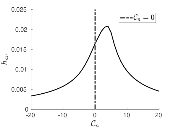
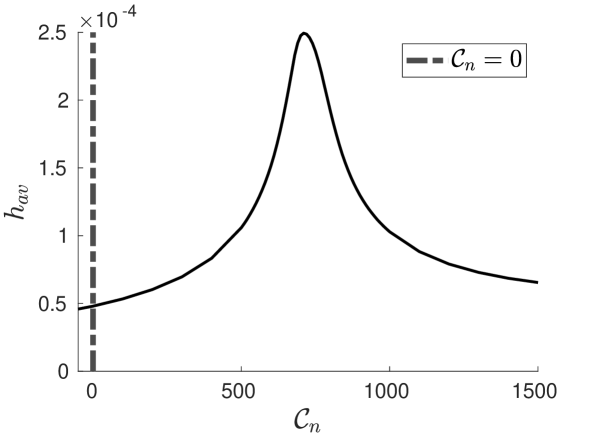
Figure 1. Average time-step $h_{av}=\textstyle{\frac{1}{N_{h}}}\sum_{n=1}^{N_{h}}h_{n}$ with a constant $\mathcal{C}_{n}$ for the IF method applied to the one dimensional NLS (left) and SN (right) equations.

Figure 2. Comparison between $\mathcal{C}_{n}=\tilde{\mathcal{C}}_{n}$ and $\mathcal{C}_{n}=0$ for time-step $h_{n}$ as a function of time, for the IF method applied to the $\mathrm{NLS_{1D}}$ (top left), $\mathrm{NLS_{2D}}$ (top right), $\mathrm{SN_{1D}}$ (bottom left) and $\mathrm{SN_{2D}}$ (bottom down).

Eq.	$\mathrm{SN_{1D}}$	$\mathrm{SN_{1D}}$	$\mathrm{SN_{2D}}$	$\mathrm{SN_{2D}}$	$\mathrm{NLS_{1D}}$	$\mathrm{NLS_{1D}}$	$\mathrm{NLS_{2D}}$	$\mathrm{NLS_{2D}}$
$\mathcal{C}$	$0$	$\tilde{\mathcal{C}}_{n}$	$0$	$\tilde{\mathcal{C}}_{n}$	$0$	$\tilde{\mathcal{C}}_{n}$	$0$	$\tilde{\mathcal{C}}_{n}$
$N_{\Delta t}$	$20819$	$3871$	$8382$	$2682$	$6047$	$4781$	$754$	$690$
$T(s)$	$66.7$	$12.1$	$12856$	$4736$	$18.9$	$14.5$	$23769$	$22843$

Table 1. Comparisons for the SN and the NLS equations, in one and two spatial dimensions, between different values of $\mathcal{C}_{n}$.

5. Conclusion

Exploiting a gauge condition on the potential, we optimized the integrating factor technique applied to the nonlinear Schrödinger and Schrödinger–Newton equations. Although the exact values of the piece-wise constant $\mathcal{C}_{n}$ minimizing the error (16) (therefore maximizing the time-step) is in principle always possible to compute (e.g., with a computer algebra system), its expression depends on the particular numerical scheme chosen and it becomes complicated as the order of the method increases, resulting in a high computational cost. However, the near-optimal value obtained from the first approach we described, based on the minimization of the $L_{2}$-norm of the nonlinear part of the equation, proved to be an accurate and efficient solution in the tested cases. Thus, being computationally extremely cheap and independent of the particular numerical scheme employed, this is the approach one should choose for most simulations, at least when the computation of $\mathcal{N}$ is not very expensive. For Schrödinger-like equations with hard to compute potentials, most of the computational time is spent in the calculation of $\mathcal{N}$. For these very demanding equations, the extra cost needed to compute the optimum $\hat{\mathcal{C}}_{n}$ (instead of the near optimum $\tilde{\mathcal{C}}_{n}$) is negligible in comparison, so $\hat{\mathcal{C}}_{n}$ could be preferable.

For the cases tested here, we found a speed-up in the computation time up to a factor $5$, the speed-up depending on the equation and on the physical regime. These examples show that this approach provides significant speed improvements, that with minor modifications of the original algorithm. Though we focused on the nonlinear Schrödinger and Schrödinger–Newton equations, the method principle is independent on the particular potential considered, so this approach can be extended to other Schrödinger-like equations. More generally, the idea behind the method presented in this note can be, at least in principle, generalized and extended to other equations with similar gauge conditions.

Appendix A Numerical simulations

For the one-dimensional NLS, we considered the case $g=-1$ (see 3) and we used $\psi(x,t=0)=\sqrt{2}\,{\mathrm{sech}}\left(\sqrt{2}\,x\right)$ as initial condition. We discretised space with $N=2048$ points, in a computational box of length $L=80$. The two-dimensional NLS, which is often employed in optics to model self-focusing beams in a medium with a cubic non-linearity [26, 27], presents a finite time (blow-up) singularity [28]. More specifically, whenever the initial condition $\psi_{0}$ satisfies $E_{g}=\int\mathrm{d}\boldsymbol{r}\,\psi_{0},\left(-\frac{1}{2}\nabla^{2}+\frac{g}{2}\left|\psi_{0}\right|^{2}\right)\psi^{*}_{0}<0$, the norm of the solution, or of one of its derivatives, becomes unbounded in finite time. For this reason, we stop the simulation at $t_{\mathrm{fin}}=5$, i.e., before the singularity occurs. We set $\psi(\boldsymbol{r},t=0)=\mathrm{e}^{-r^{2}/2}/\sqrt{\pi}$ as initial condition and we consider the $g=-6$ case, for which the corresponding initial energy is $E(g=-6)\approx 0.02$, hence quite close to the singular regime; for the spatial discretization we used $L=120$ and $N=4096^{2}$ (squared box with side $L=120$ discretised with $4096\times 4096$ nodes). For both the one and two dimensional SN equations, we set $g=500$ and considered a Gaussian initial condition, $\psi(\boldsymbol{x},t=0)=\mathcal{N}\mathrm{e}^{-\left|\boldsymbol{x}\right|^{2}/2}$ where $\mathcal{N}$ is the normalization factor, fixed such that $\int\mathrm{d}\boldsymbol{x}\left|\psi(\boldsymbol{x},t=0)\right|^{2}=1$. The parameters of the spatial discretization are $L=20$ and $N=2048$ in 1D, while for the 2D case we set $L=20$ and $N=1024^{2}$. To solve the SN and the NLS equation we used the Dormand and Prince 5(4) integrator [22].

References

- [1] Franco Dalfovo, Stefano Giorgini, Lev P Pitaevskii, and Sandro Stringari. Theory of Bose–Einstein condensation in trapped gases. Reviews of Modern Physics, 71(3):463, 1999.
- [2] Akira Hasegawa. Optical solitons in fibers. In Optical Solitons in Fibers, pages 1–74. Springer, 1989.
- [3] Christian Kharif, Efim Pelinovsky, and Alexey Slunyaev. Rogue waves in the ocean. Springer Science & Business Media, 2008.
- [4] James Binney and Scott Tremaine. Galactic Dynamics: Second Edition. 2008.
- [5] FW Dabby and JR Whinnery. Thermal self-focusing of laser beams in lead glasses. Applied Physics Letters, 13(8):284–286, 1968.
- [6] Carmel Rotschild, Oren Cohen, Ofer Manela, Mordechai Segev, and Tal Carmon. Solitons in nonlinear media with an infinite range of nonlocality: first observation of coherent elliptic solitons and of vortex-ring solitons. Physical review letters, 95(21):213904, 2005.
- [7] Carmel Rotschild, Barak Alfassi, Oren Cohen, and Mordechai Segev. Long-range interactions between optical solitons. Nature Physics, 2(11):769–774, 2006.
- [8] F Siddhartha Guzman and L Arturo Urena-Lopez. Gravitational cooling of self-gravitating Bose condensates. The Astrophysical Journal, 645(2):814, 2006.
- [9] Wayne Hu, Rennan Barkana, and Andrei Gruzinov. Fuzzy cold dark matter: the wave properties of ultralight particles. Physical Review Letters, 85(6):1158, 2000.
- [10] Angel Paredes and Humberto Michinel. Interference of dark matter solitons and galactic offsets. Physics of the Dark Universe, 12:50–55, 2016.
- [11] David JE Marsh and Jens C Niemeyer. Strong constraints on fuzzy dark matter from ultrafaint dwarf galaxy Eridanus ii. Physical review letters, 123(5):051103, 2019.
- [12] Lajos Diosi. Gravitation and quantumm-echanical localization of macroobjects. arXiv preprint arXiv:1412.0201, 2014.
- [13] Roger Penrose. On gravity’s role in quantum state reduction. General relativity and gravitation, 28(5):581–600, 1996.
- [14] Lawrence M Widrow and Nick Kaiser. Using the Schrödinger equation to simulate collisionless matter. The Astrophysical Journal, 416:L71, 1993.
- [15] C. Canuto, M. Y. Hussaini, A. Quarteroni, and Th. A. Zang. Spectral Methods. Fundamentals in Single Domains. Scientific Computation. Springer, 2nd edition, 2008.
- [16] J Douglas Lawson. Generalized Runge–Kutta processes for stable systems with large Lipschitz constants. SIAM J. Numer. Anal., 4(3):372–380, 1967.
- [17] Sergio Blanes, Fernando Casas, and Ander Murua. Splitting and composition methods in the numerical integration of differential equations. arXiv preprint arXiv:0812.0377, 2008.
- [18] Philipp Bader, Sergio Blanes, Fernando Casas, and Mechthild Thalhammer. Efficient time integration methods for Gross–Pitaevskii equations with rotation term. arXiv preprint arXiv:1910.12097, 2019.
- [19] Christophe Besse, Geneviève Dujardin, and Ingrid Lacroix-Violet. High order exponential integrators for nonlinear Schrödinger equations with application to rotating Bose–Einstein condensates. SIAM J. Numer. Anal., 55(3):1387–1411, 2017.
- [20] Roger Alexander. Solving ordinary differential equations i: Nonstiff problems (e. hairer, sp norsett, and g. wanner). Siam Review, 32(3):485, 1990.
- [21] John Charles Butcher. Numerical methods for ordinary differential equations. John Wiley & Sons, 2016.
- [22] John R Dormand and Peter J Prince. A family of embedded Runge–Kutta formulae. J. Comp. Appl. Math., 6(1):19–26, 1980.
- [23] Endre Süli and David F Mayers. An introduction to numerical analysis. Cambridge university press, 2003.
- [24] Gerhard Wanner and Ernst Hairer. Solving ordinary differential equations II. Springer Berlin Heidelberg, 1996.
- [25] Kjell Gustafsson. Control theoretic techniques for stepsize selection in explicit Runge–Kutta methods. ACM Transactions on Mathematical Software (TOMS), 17(4):533–554, 1991.
- [26] VE Zakharov and VS Synakh. The nature of the self-focusing singularity. Zh. Eksp. Teor. Fiz, 68:940–947, 1975.
- [27] Kimiaki Konno and Hiromitsu Suzuki. Self-focussing of laser beam in nonlinear media. Physica Scripta, 20(3-4):382, 1979.
- [28] Catherine Sulem and Pierre-Louis Sulem. The nonlinear Schrödinger equation: self-focusing and wave collapse, volume 139. Springer Science & Business Media, 2007.