22 \papernumber2126
Morphisms and Minimisation of Weighted Automata
Morphisms and Minimisation of Weighted Automata
Abstract
This paper studies the algorithms for the minimisation of weighted automata. It starts with the definition of morphisms — which generalises and unifies the notion of bisimulation to the whole class of weighted automata — and the unicity of a minimal quotient for every automaton, obtained by partition refinement.
From a general scheme for the refinement of partitions, two strategies are considered for the computation of the minimal quotient: the Domain Split and the Predecesor Class Split algorithms. They correspond respectivly to the classical Moore and Hopcroft algorithms for the computation of the minimal quotient of deterministic Boolean automata.
We show that these two strategies yield algorithms with the same quadratic complexity and we study the cases when the second one can be improved in order to achieve a complexity similar to the one of Hopcroft algorithm.
1 Introduction
The main goal of this paper is to report on the design and analysis of algorithms for the computation of the minimal quotient of a weighted automaton.
The existence of a minimal deterministic finite automaton, canonically associated with every regular language is one of the basic and fundamental results in the theory of classical finite automata [1]. The problem of the computation of this minimal (deterministic) automaton has given rise to an extensive literature, due to the importance of the problem, both from a theoretical and practical point of view. The chapter Minimisation of automata of the recently published Handbook of Automata Theory [2] is devoted to this question by Jean Berstel and his colleagues [3]. It provides a rich and detailed account on the subject, together with an extensive list of references.
In contrast, the problem of minimisation of nondeterministic Boolean, or of weighted, automata is much less documented. The chapter Algorithms for weighted automata in the Handbook of Weighted Automata [4] deals only with the case of so-called deterministic weighted automata on which the algorithms for deterministic Boolean automata can be generalised. The main reason is probably that the problem of finding a (Boolean) automaton equivalent to a given automaton and with a minimal number of states is untractable and known to be NP-hard and even PSPACE-complete [5]. Of course, the case of weighted automata, with arbitrary weight semiring, is at least as difficult.
There is another way to look at the minimisation of deterministic Boolean automata. The result, the minimal automaton, is obtained by merging states and in this way can be seen as the image of the original automaton by a map that preserves the structure of the computations, a map it is natural to call morphism. The other purpose of this paper, which indeed comes first, is then to set up the definition of morphisms for arbitrary (finite) weighted automata, and in particular for nondeterministic Boolean automata. The image of a morphism is a quotient and, as in the original case, an automaton has a unique minimal quotient (Theorem 3.12). The difference with the original case is that the minimal quotient is not canonically attached to the series or the language realised by the automaton but to the automaton itself.
To tell the truth, this point of view is not completely new. For transition systems for instance, which are automata without initial and final states, it is common knowledge that the notion of bisimulation allows to merge states in order to get a system in which the computations are preserved and the coarsest bisimulation yields a minimal system. The notion of bisimulation has also been extended to some classes of weighted automata, for instance probabilistic automata [6], or automata with weights in a field or division ring [7]. It is also known that in all these cases the coarsest bisimulation is computed by iterative refinements of set partitions.
We show here that the classical algorithms of partition refinement that are used for deterministic Boolean automata (widely known as Moore and Hopcroft algorithms) may be analysed and abstracted in such a way they readily extend to weighted automata in full generality, without any assumption on the weight semiring and on the automaton structure. This can be sketched as follows. In a partition refinement algorithm, and at a given step of the procedure, a partition of the state set of an automaton, and a class of are considered. There are then two possible strategies for determining a refinement of . In the first one, the class itself is split, by considering the labels of the outgoing transitions from the different states in . This is an extension of the Moore algorithm and we call it the Domain Split Algorithm. In the second strategy, the class determines the splitting of classes that contain the origins of the transitions incoming to the states in . We call it the Predecessor Class Split Algorithm and it can be seen as inspired by the Hopcroft algorithm.
Although the two strategies yield distinct orderings of the splitting of classes, the two algorithms have many similarities that we describe in this paper. Not only do they have the same time complexity, in , where is the number of states of the automaton and the number of its transitions, but the criterium for distinguishing states — the splitting process — is based on the same state function that we call signature. And in both cases, achieving the above mentioned complexity implies that signatures are managed through the same efficient data structure that implements a weak sort.
Finally, our analysis allows to describe a condition — which we call simplifiable signatures — under which the Predecessor Class Split Algorithm can be tuned in such a way it achieves a better time in , the Graal set up by Hopcroft algorithm for deterministic Boolean automata (in which , where is the size of the alphabet).
In conclusion, our study of the minimisation algorithms, with the identification of the concept of signature, allows to reverse the perspective. We have not transformed the known algorithms on deterministic Boolean automata by equipping them with supplementary features that allow to treat weighted automata, we have just expressed them in a way they can deal with all weighted automata and they apply then to deterministic Boolean automata just as they do with any other, not even in a simpler way.
The paper is organised as follows. In Section 2, we begin with the definitions and notation used for weighted automata. We add the definition of a special class of automata, a kind of normalised ones, which we call augmented automata and which will be useful for the writing of algorithms. At Section 3, we give two equivalent definitions for morphisms of weighted automata and show the existence of a unique minimal quotient.
In Section 4, we describe a general procedure for the partition refinement, the notion of signature, and both the Domain Split and Predecessor Class Split Algorithms. In the next Section 5, we describe the way to implement the weak sort, how it is used in the two algorithms, and we analyse their complexity, whereas we explain in Section 6 under which conditions and how it is possible to improve the complexity of the latter.
The algorithms and their efficient implementation described in this paper are accessible in the Awali plateform recently made available to the public [8]. Some experiments presented at Section 7 show that the algorithms behave with their theoretical complexity. These experiments were presented at the CIAA conference in 2018 [9].
2 Weighted automata
In this paper, we deal with (finite) automata over a free monoid with weight in a semiring , also called -automata. ‘Classical’ automata are the -automata where is the Boolean semiring.
Indeed, all what follows apply as well to automata over a monoid which is not necessarily free, for instance to transducers that are automata over the non free monoid . This generalisation holds as such automata are considered — as far as the constructions and results developped here are concerned — as automata over a free monoid , where is the set of labels on the transitions of the automaton. Let us note that there exists no theory of quotient that takes into account non trivial relations between labels. The only construction on automata that does (without destroying their structure) is the circulation of labels involved for instance in the synchronisation of transducers (cf. [10, 11]) or as a preliminary for the minimisation of sequential transducers (cf. [10, 12]).
2.1 Definition and notation
We essentially follow the definitions and notation of [10]. The model of weighted automaton used in this paper is more restricted though, for both theoretical and computational efficiency.
A -automaton over is a directed graph whose vertices are called states and whose edges, called transitions, are labelled by a pair made of a letter in and a weight in , together with an initial function and a final function, both from the set of states to . The states in the support of the initial function are usually called initial states, those in the support of the final function, final states. Figure 1 shows a -automaton over with the usual graphical conventions.
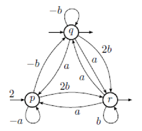
Let be a -automaton with set of states ; we say that is the dimension of and we denote by a triple where and are vectors of dimension with entries in that denote the initial function and the final functions and is the adjacency matrix of , that is, a -matrix whose entry is the sum of the weighted labels of the transitions from to . We also denote by the map and is the weight of the (unique) transition that goes from to and that is labelled by , if it exists (otherwise its value is ).
Example 2.1
Let of dimension :
The behaviour of a -automaton is the series realised by and is denoted by :
where (the infinite sum does not bring any problem as our definition insures that the entries of are homogenous polynomials of degree ). Two automata are said to be equivalent if their behaviours are equal. If , is the language accepted by .
The future of a state of , denoted by , is the series realised by when is taken as the unique initial state, with initial value equal to . It holds
| (1) |
where denotes the characteristic (row-) vector of , that is, the entry of index is the only non-zero entry and is equal to .
2.2 The augmented automaton
The algorithms we describe and study in the following sections classify states of an automaton according to (the labels of) the in- and out-going transitions and (the values of) the initial and final functions. In order to express in the same way the conditions stated on the transitions on one hand and on the initial and final functions on the other, and to compute uniformly with the former and the latter, it is convenient to transform the automaton and to put them in a special form which we call augmented.
A -automaton of dimension over is transformed into its augmented version, denoted by , in two steps. First, the alphabet is supplemented with a new letter , which will be used as a left and right marker. We write for , the augmented alphabet. Second, is somehow normalised by the adjunction of two new states and to and of transitions that go from to every initial state with label and with weight and transitions that go from every final state to with label and with weight . As it will be useful to make its state set explicit, we denote by where contains the complete description of , as seen in (2).
| (2) |
Finally, the only initial state of is , with weight , and its only final state is , also with weight . If is in , there is a 1-1 correspondence between the successful computations with label in and the computations with label in , hence they are given the same weight by the two automata. Hence, .
Example 2.2 (continued)
The adjacency matrix of the -automaton is shown on Figure 2. There is no column nor row in the table for there is no transitions incoming to nor transitions outgoing from .
3 Morphisms of weighted automata and minimal quotients
The notion of morphism for deterministic Boolean automata does not raise difficulties and makes consensus. In contrast, the one of morphism for arbitrary Boolean automata and even more for (arbitrary) weighted automata is far more problematic. In most cases, the concept is given other names, most often simulation or bisimulation, when not more complicated such as weak bisimulation or pure epimorphism, and definitions that may depend on the case considered and hide their generality.
3.1 Amalgamation matrices and morphisms
We start with the definition of morphisms — of Out-morphisms indeed as we shall see — by means of the notion of conjugacy of automata, as we already did in [10] or [13] and which is the most concise one. We then translate it into a more explicit definition via equivalence that is more suited for computations.
Definition 3.1
Let and be two -automata, of dimension and respectively. We say that is conjugate to by if there exists a -matrix with entries in such that
| (3) |
The matrix is the transfer matrix of the conjugacy and we write .
If is conjugate to , then, for every , the sequence of equalities holds:
from which directly follows. And this is stated as the following.
Proposition 3.2
If is conjugate to , then and are equivalent. \squareforqed
The conjugacy relation is not an equivalence relation as it is reflexive and transitive but not symmetric.
A surjective map is completely described by the -matrix whose -th entry is if , and otherwise. Since is a map, every row of contains exactly one and since is surjective, every column of contains at least one . Such a matrix is called an amalgamation matrix in the setting of symbolic dynamics ([14]). By convention, if we deal with -automata, an amalgamation matrix is silently assumed to be a -matrix, that is, the null entries are equal to and the non-zero entries to .
Definition 3.3
Let and be two -automata of dimension and respectively. A surjective map is a morphism (from onto ) if is conjugate to by : , that is,
| (4) |
and we write .
We also say that is a quotient of , if there exists a morphism .
It is straightforward that the composition of two morphisms is a morphism. And by Proposition 3.2, any quotient of is equivalent to .
Definition 3.3 may be given a form which will probably be more eloquent to many than a mere matrix equation, and which makes clear that the automaton , and its state set , are immaterial and that the conditions are upon and the map equivalence of only. Above all, it will be the one used in the design of the algorithms to come. We describe it in the next subsection.
3.2 Morphisms and congruences
We start with some definitions and notation to deal with equivalences. An equivalence on a set is a partition of , that is, a set of non-empty disjoint subsets of , called classes, whose union is equal to . If is an equivalence on , we denote by both the set of classes in the partition as well as the relation on determined by the partition, that is, for every pair of elements of , if and only and belong to a same class of .
Equivalences and surjective maps are indeed the same objects, seen from a slightly different perspective. An equivalence on determines the surjective map that sends every in onto its class modulo and conversely every surjective map determines the map equivalence. In both cases, they are represented by amalgation matrices.
Let us introduce a last definition. Let be an equivalence on and its amalgamation matrix. From we construct a selection matrix by transposing and by zeroing some of its non-zero entries in such a way that is row-monomial, with exactly one per row. A matrix is not uniquely determined by but also depends on the choice of the entry which is kept equal to , that is, of a ‘representative’ in each class of .
Definition 3.4
Let be an automaton of dimension . We call congruence on the map equivalence of a morphism from onto an automaton .
Proposition 3.5
Let be a -automaton over of dimension . An equivalence on is a congruence if and only if the following holds:
| (5) | ||||
| (6) |
Proof 3.6
The condition is necessary. Let be a quotient of , a morphism, and its map equivalence. The multiplication of on the right by amounts to add together the columns of whose indices are sent to a same element by , that is, indices which are in a same class of . The entries of the -matrix are:
| (7) |
Every is a linear combination of letters of : and (7) may be rewritten as
| (8) |
On the other hand, the multiplication of , on the left, by yields a matrix whose rows with indices in the same class modulo are equal. Hence the equality implies (5). For the same reason, implies (6).
The condition is sufficient. Let be an equivalence on such that (5) and (6) hold, its amalgamation matrix, and a selection matrix.
The entries of are indexed by , and is a (column-) vector of dimension obtained by picking one entry of in each class modulo . The vector , of dimension , is obtained by replicating, for every in , the entry of indexed by for each of in . Since (6) expresses that all entries of indexed by states in a same class are equal, holds.
In the same way, the rows (of dimension ) of are indexed by , and is a -matrix obtained by picking one row of in each class modulo . The matrix , of dimension , is obtained by replicating, for every in , the row of indexed by for each of in . Since (5) expresses that all rows of indexed by states in a same class are equal, holds.
Remark 3.7
As mentioned in the introduction, morphisms have a close relationship with bisimulations. One can even say it is the same notion expressed differently, for those weighted automata for which bisimulations have been defined: bisimulations for transition systems which are Boolean automata without initial and final states [15, 16], for probabilistic systems [17, 6], linear bisimulations when the weight semiring is a field [7], etc. and when it is freed from so-called internal actions.
Indeed an equivalence relation on the state set of an automaton is a bisimulation relation if and only if it is a congruence. And a state of is in bisimulation with its image in any quotient of .
Example 3.8 (continued)
Let of dimension :
It is easily seen that if we add the columns and of we get a matrix whose rows and are equal; moreover . Hence is a congruence of .
Since it is characteristic, we could have taken just as well the statement of Proposition 3.5 as the definition of a congruence or a morphism. And all the more in this paper where it is the property which is uniformly called. But in view of further references to this paper, we prefer to put Definition 3.3 in front, for its mathematical efficiency (e.g. [18]).
3.3 Further properties of morphisms and congruences
Proposition 3.9
Let be a -automaton over of dimension and a congruence on . If two states and are equivalent modulo , then .
Proof 3.10
With the notation of Section 2, and with the same computation as above, . Accordingly, . And if and are equivalent modulo , then .
Remark 3.11
Definition 3.3 gives a notion of morphism that is directed as the one of conjugacy is: is multiplied on the right by in (3). This is even more obvious with the statements of Proposition 3.5 or of Proposition 3.9.
Thus morphisms could, or should, be called Out-morphisms as it refers to out-going transitions. The same map would be an In-morphism if is conjugate to by (the transpose of ).
In this work, we deal with Out-morphisms only, which we simply call morphisms. All statements can be dualised and transformed accordingly for In-morphisms.
Remark 3.12
The case of Boolean automata. Let and be two Boolean automata over of dimension and respectively and a morphism from to . In this special case, no weight is really involved: a transition exists or not, a state is initial or not, final or not. Moreover, and can also be seen as subsets of , and as subsets of , can also be seen as a subset of , as a subset of . Definition 3.3 can then be rewritten in the following way: and translate into
whereas yields
| (iii) | |||||
| (iv) |
Compared with previous terminology, morphisms of Boolean automata as we have just defined them are what we have called locally surjective Out-morphisms in [10] and subsequent works. In the case of deterministic Boolean automata, our definition coincide with the classical notion of morphisms of automata, when it is used.
Remark 3.13
The case of augmented automata. If is a morphism, then is also a morphism, where , , and , , and for all in . This amounts to say that has the form
| (9) |
a matrix which we rather denote by .
Conversely, if is the augmented automaton of , the amalgamation matrix of any morphism of is of the form (9) and corresponds to a morphism of . In particular, if is an augmented -automaton, an equivalence on is a congruence on if and only if
| (10) | |||
| (11) |
3.4 Minimal quotients
With Definition 3.3, we have defined the quotients of a -automaton . The following proposition states that every -automaton has a minimal quotient.
Theorem 3.14
Among all quotients of a -automaton , there exists one, unique up to isomorphism, which has a minimal number of states and which is a quotient of every quotient of .
Once again, it is convenient to express this property in terms of congruences, which focuses on the automaton itself rather than on its images. It starts with the definition of an order on equivalences, or partitions, on a set .
An equivalence is coarser than an equivalence if, for every in , there exists in such that is a subset of . It follows that every class of is the union of classes of . The equivalences on a set , ordered by this inclusion relation, form a lattice, with the identity — where every class is a singleton — at the top and the universal relation — with only one class that contains all elements of — at the bottom. The following is then a statement equivalent to Theorem 3.14.
Theorem 3.15
Every -automaton has a unique coarsest congruence.
Indeed, the equivalence map of the morphism onto the minimal quotient is the coarsest congruence and the coarsest congruence is the equivalence map of the morphism onto the minimal quotient.
Remark 3.16
It is important to stress once again that the minimal quotient of is associated with , and not with the series realised by . It is not necessarily the smallest (in terms of number of states) -automaton that realises the series, it is not a canonical automaton associated with it.
For instance, the minimal quotient of a Boolean automaton is not necessary the smallest automaton for the accepted language. On the other hand, the minimal quotient of a deterministic Boolean automaton is the minimal (deterministic) automaton of the accepted language (which may well be larger than another Boolean automaton accepting the same language) that is, the notion we have defined for all (possibly weighted) automata coincides with the classical one in the case of deterministic Boolean automata.
Proof 3.17 (Proof of Theorem 3.14)
Let be a -automaton of dimension . The proof of the existence of a coarsest congruence on goes downward, so to speak, that is, we start from the identity on which is a congruence. Let and be two morphisms. In order to prove the existence of a minimal quotient (or of a coarsest congruence) it suffices to verify that the lower bound of the map equivalences of and is a congruence. Let and such that . Hence
| (12) |
By definition, two states and of are equivalent modulo , which we write , if and only if there exists a sequence of states of such that and for . Rows of indices and of , and then of , are equal, rows of indices and of , and then of , are equal, hence rows of indices and of are equal. For the same reason, and is a congruence.
Remark 3.18
In the case of Boolean automata also, the characterisation of bisimulation follows from Remark 3.7.
Proposition 3.19
Two -automata are bisimilar if and only if their minimal quotients are isomorphic. \squareforqed
The minimal quotient not only exists but is also effectively, and efficiently computable, as we see in the next sections.
4 The computation of the minimal quotient
To describe the algorithms computing the minimal quotient of a weighted automaton, it is convenient to consider the augmented automaton. From now on, every automaton is therefore augmented, the alphabet is , and the states which are different from the initial or final states are called true states.
4.1 Refinement algorithms and signatures
The principle of algorithms which are studied in this paper is partition refinement. The algorithms start with the coarsest equivalence (where all true states are gathered in one class), and split classes which are inconsistent with the constraints of a congruence. In order to split classes, we use a criterion on states of , which we call signature, and which, given a partition, tells if two states in a same class should be separated in a congruence of . This notion of signatures has been used in [19] for the minimisation of incomplete deterministic Boolean automata, the ‘first’ example for which the classical minimisation algorithms for complete deterministic Boolean automata have to be adapted.
The signature is first defined with respect to a class.
Definition 4.1
The signature of a state of a -automaton with respect to a subset of is the map from to , defined by:
For every state and every subset , the domain of is the set of labels of transitions from to some state of . In particular, if a letter does not belong to the domain of , then . When we want to explicitly describe , we write it as a set of elements of the form , where is in the domain of and .
Two states and cannot be equivalent with respect to some congruence of if their signatures differ for some class of . In order to compare states, it can be useful to consider the global signature which is the aggregation of signatures with respect to all classes of the partition. That is, for a given partition and for every state ,
4.2 The Protoalgorithm
The computation of the coarsest congruence of an automaton goes upward. It starts with , the coarsest possible equivalence. Every step of the algorithm splits some classes of the current partition, yielding an equivalence which is thiner, higher in the lattice of equivalences of .
It follows from Proposition 3.5 that a partition is a congruence if and only if
Thus is a congruence if and only if, for every pair of classes of , all states in have the same signature with respect to . A pair for which this property is not satisfied is called a splitting pair. The equivalence on induced by the signature with respect to , called the split of by and denoted by , can be computed:
The split of class by class of leads to a new equivalence on : , and the protoalgorithm runs as follows:
| while there exists a splitting pair in | |
When there are no more splitting pairs, the current equivalence is a congruence.
Proposition 4.2
At every iteration of the protoalgorithm, the equivalence is coarser than or equal to the coarsest congruence.
Proof 4.3
In the initial partition , all true states are in the same class, thus is coarser than or equal to any congruence.
Let be a partition computed at one iteration; we assume that is coarser than or equal to the coarsest congruence , and we consider computed at the next iteration. There exists a splitting pair , such that . If is not coarser than or equal to , then there exists and in , in and in which belongs to the same class in . Since is coarser than or equal to , is the union of some classes in ; and are -equivalent, hence, for every ,
| (13) |
Therefore, , which is in contradiction with the fact that and are in different classes after the split of with respect to . Thus is coarser than or equal to and, by induction, the proposition holds.
Corollary 4.4
At the end of the protoalgorithm, the equivalence is equal to the coarsest congruence. \squareforqed
The procedure described by the protoalgorithm is not a true algorithm, in the sense that, in particular, it does not tell how to find a splitting pair, nor how to implement the function to make it efficient. The main difference between the two algorithms described in the sequel is the selection of the splitting pairs.
-
•
the first algorithm iterates over classes and considers in the same iteration all the pairs where is any class which contains some successors of states of . This leads to split in classes which are consistent with every class . We call it the Domain Split Algorithm (DSA for short).
-
•
the second algorithm iterates over classes and considers in the same iteration all the pairs where is any class which contains some predecessors of states of . This leads to split several classes in such a way that all classes become consistent with the class . We call it the Predecessor Class Split Algorithm (PCSA for short).
4.3 The Domain Split Algorithm
The Domain Split Algorithm is an extension of the classical Moore algorithm [20] for the minimisation of deterministic Boolean automata. At each iteration of this algorithm, a class is processed. The global signature of every state of with respect to the current partition is computed, and is split accordingly. Compared to the protoalgorithm, the Domain Split Algorithm amounts therefore to consider at the same time all the pairs , where is the current class, and is any class of the current partition (actually, only classes which contain some successors of states of are considered). Notice that it is mandatory to recompute signatures at each iteration, since they depend on the partition which is changing.
At the beginning of each iteration, the current class is extracted from a queue. At the beginning of the algorithm, the partition is , and is inserted in the queue. At the end of each iteration, the classes obtained from the split of — or itself if it has not been split — are inserted into the queue, except the singletons that cannot be split.
To insure termination, iterations are gathered to form rounds. A round ends when all classes that were inside the queue at the beginning of the round have been extracted. Hence the number of iterations in a round is equal to the number of classes which are in the queue at the beginning of the round. Notice that, for every state , there is at most one class containing that is processed during a round. If there is no split during a round, the algorithm has checked that the partition is a congruence and halts.
Otherwise, the partition is strictly refined and the number of classes strictly increases. At the beginning of the algorithm, there are three classes, and the maximal number of classes is , where is the number of true states of the automaton. Hence, including the last round, there are at most rounds, and, for every state, at most global signatures are computed.
Example 4.5 (continued)
On the automaton , the partition is initialised with , , . Class is put into the queue (the other classes are singletons and cannot be split). For every state of and for every class , one can compute the signature of this state with respect to . For instance, the signature of with respect to is
From the signature with respect to each class, the global signature of the state can be computed.
The global signature (with respect to ) of states in is:
States and share the same global signature which is different from the global signature of . The class is then split into two classes and and the new partition is . The new round starts and the class is put in the queue. The global signature of states (with respect to ) in is:
Both states have the same global signature, thus the class is not split. The round ends without any splitting, hence the current partition is a congruence.
4.4 Predecessor Class Split Algorithm
The Predecessor Class Split Algorithm is inspired by the Hopcroft algorithm for the minimisation of deterministic Boolean automata. At each iteration of this algorithm, a class is processed. For every state which is a predecessor of some states of , the signature of with respect to is computed, and is split accordingly. Compared to the protoalgorithm, PCSA amounts therefore to consider at the same time all the pairs , where is the current class, and is any class of the current partition (actually, only classes which contain some predecessors of states of are considered).
Like the DSA, the PCSA uses a queue to schedule the process of classes. At the beginning of the algorithm, every class of is put into the queue, except since there is no predecessor of . If a class is split, every new class is put in the queue; if was in the queue, it is replaced by its subclasses. The algorithm halts when the queue is empty. Actually, when the partition is a congruence, every class extracted from the queue does not induce any splitting, hence there is no more insertion of classes.
Apart from the initialisation of the queue, every class which is inserted in the queue comes from a split. Hence, for every state , the number of times that a class containing is extracted from the queue is at most equal to , where is the number of true states of the automaton. Notice that there is no notion of rounds in the PCSA.
Example 4.6 (continued)
On the automaton , the equivalence is initialised with , , . Classes and are put in the queue ( has no predecessor, thus can not split any class). Assume that is considered first. The signatures of predecessors of states in are:
All states in the class have the same signature ( is a singleton!). In the class , every state is met, but has a signature which is different from the signature common to and . Hence is split into two classes and which are inserted in the queue.
The next class which is extracted from the queue is , and the signatures of predecessors of states in are:
Both states have the same signature and there is no other state in , thus there is no split.
The class processed in the next iteration is , and the signatures of predecessors of states in are:
States and are already in classes which are singletons; states and have the same signature and there is no other state in , thus there is no split.
The next processed class is , and the signatures of predecessors of states in are:
States and are already in classes which are singletons; states and have the same signature and there is no other state in , thus there is no split.
The queue is empty; the algorithm halts and the current partition is a congruence.
5 Complexity of the refinement algorithms
The high-level description of the DSA and PCSA have shown that every state is processed at most times, where is the number of true states. Processing a state consists in running over its outgoing transitions (for DSA) or its incoming transitions (for PCSA) to compute signatures. Globally, every transition of the automaton is thus considered at most times.
To be efficient, the time to compute the signatures must be linear in the number of transitions involved in the computation. The key point in the algorithms is the ability to compute signatures in such a way that the signatures of two states can be compared in linear time. Usually, to compare two lists efficiently, a preliminary step consists in sorting them. To reach the linear complexity, a true sort is not affordable. Hence, we present here a weak sort [21] which allows to compare signatures in linear time.
5.1 The weak sort
Let be an evaluation function from a set to a set . In our framework, the evaluation function is the signature. If is totally ordered, sorting a list of elements of with respect to consists in computing a permutation of the list such that the elements of the list are ordered with respect to the evaluation . If such a list is sorted, the elements with the same evaluation are contiguous and it is then easy to gather them. Following the ideas given in [21], it is not necessary to fully sort the list, and we say that a list of elements of is weakly sorted (with respect to ) if the elements with the same evaluation by are contiguous. It is then easy to compute the map equivalence of .
Both DSA and PCSA are based on a weak sort with respect to signatures. Since signatures are themselves lists, nested weak sorts are necessary to gather states with the same signatures such that equal signatures are represented by the same lists.
In a first step, and for every state , transitions outgoing from with the same label and with destinations in the same class must be gathered.
Moreover, for two states with the same signature, the list of pairs (label weight) that form the signature must appear in the same ordering, in such a way the equality test is insured to be efficient.
In a second step, the weak sort is used to gather states with the same signature and to form the new classes.
A bucket sort algorithm [22] realises a weak sort with linear complexity in the size of . Assume first that arrays indexed by can be managed. Let be such an array where elements are lists of values in . The algorithm iterates over and stores every in in the list . Finally, by iterating over , all the lists are concatenated in order to compute a weakly sorted list.
This naive description hides two issues. First, may be large, and the initialisation of every element of to the empty list is linear in , which can be much larger than . The second issue is related to the first one, there may be a few in which are images of some by , and it is too expensive to iterate over all elements of to concatenate the lists.
The hash maps are a solution to the first issue (see [23, 22] for instance). They allow to avoid the blowing up of memory in the case where is huge. As the amortised access time is constant, it allows to implement the weak sort in linear time. To solve the second issue, the keys of the hash map can be linked in order to efficiently iterate over the elements of (the data structure is then equivalent to the linked hash maps implemented for instance in Java [24]).
5.2 Application to the Domain Split Algorithm
The computation of the global signature of the states of the current class requires two steps.
First, an array indexed by stores lists of pairs in . For every state in , and for every transition , the pair is inserted in a list , where is the class of . This insertion is special in the case where is not empty and its last element is a pair with : is then updated to ; if is zero, the pair is removed from the list. The second step builds the global signature itself. For every useful index , for every in , inserts into .
We see that the elements in follow an ordering which is consistent with the ordering of iteration on . Two states with the same global signatures have therefore the same list.
5.3 Application to the Predecessor Class Split Algorithm
For PCSA, the computation of the signature is slightly easier. The first array is only indexed by . For each in , for every transition , is inserted in a list . Then, for every key of , for every in , is inserted in with the same special insertion used in DSA. Notice that this special insertion occurs here in the second step whereas it is used in the first step in DSA.
5.4 Splitting of classes
In DSA the current class is split, the signature of every state of the class is considered, and it is not difficult to split the class in linear time with respect to its size.
In PCSA the current class is the splitter; it may induce the splitting of several classes, and all the operations must be performed in a time which is linear with respect to the number of transitions incoming to states of . In particular, the splitting of a class must be performed in a time which is linear with the number of the states which are predecessors of a state of — that may be much smaller than the size of the class.
To this end, it is required that the deletion of any element of a class can be performed in constant time. Thus classes are implemented by double linked lists, and an array indexed by states gives, for each state, a pointer to the location of the state in its class.
5.5 Analysis of both algorithms
In DSA, as seen in Section 4.3, every state may be considered times, where is the number of states. The computation of the global signature of a state requires a number of operations which is linear with the number of transitions outgoing from this state. Every iteration requires a time which is linear with the number of transitions outgoing from the current class. Finally, the time complexity of DSA is in , where is the number of states and is the number of transitions of the automaton, provided that each operation and the computation of a hash for the weights is in constant time.
In PCSA, every state may be considered times. The computation of the signatures during an iteration is linear with the number of transitions incoming to the current class. Finally, the time complexity of PCSA is in , under the same conditions as above.
Theorem 5.1
The Domain Split Algorithm and the Predecessor Class Split Algorithm compute the minimal quotient of a -automaton with states and transitions in time .
In the case of a deterministic Boolean automaton, where , with , we get back to the classical complexity of the Moore minimisation algorithm (cf. [1, 3] for instance). It may seem strange that PCSA which has been said to be inspired by Hopcroft’s algorithm has the same complexity. This is explained in the next section.
6 Conditions for an algorithm
Hopcroft’s algorithm can be seen as an improvement of PCSA for complete Boolean deterministic automata. Its time complexity is (cf. for instance [25, 26]), where is the size of the alphabet; this algorithm has been extended to incomplete DFA [19, 27] with complexity .
The strategy: “All but the largest”, introduced in [28], can be applied to improve PCSA in some cases that we now study.
At every step of PCSA, some classes are evaluated (through signatures) with respect to the current splitter . If the class is split into several classes, , all these classes are processed as splitters in further iterations.
The idea of the “All but the largest” strategy is that it is useless to process the last of the subclasses of because after the splits induced by itself and the splits induced by all the other subclasses, this subclass does not induce any new split. If this is true, one can choose which subclass is not processed; in order to get a better complexity, the strategy commands to choose the larger one.
6.1 Simplifiable signatures
A sufficient condition to apply this strategy is that the signatures with respect to the last subclass can be deduced from the signatures with respect to and the signatures with respect to the other subclasses.
The signatures are equipped with the pointwise addition: for every in ,
and if is a subset of and a partition of , then it holds:
Definition 6.1
An automaton has simplifiable signatures if, for every subset of and every subset of , and for every pair of states , it holds
A commutative monoid is cancellative if for every , , and in , implies . In particular, every group is cancellative, and if is a ring, the additive monoid is cancellative.
Lemma 6.2
Let be a semiring such that the additive monoid is cancellative. Then every -automaton has simplifiable signatures.
For other weight semirings, the simplifiability of signatures depends on the automaton. If is a deterministic111called sequential in [10]. -automaton, that is, if for every state and every letter , there is at most one transition outgoing from with label , then the signatures are simplifiable, independently of , since it holds:
Typically, incomplete deterministic Boolean automata, as considered in [19], have simplifiable signatures whereas general Boolean automata have not.
Example 6.3
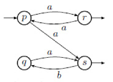
Let be the nondeterministic Boolean automaton of Figure 3. It holds:
The signature with respect to cannot be deduced from the signature with respect to and . Hence, has not simplifiable signatures.
6.2 The “All but the largest” strategy
If is an automaton with simplifiable signatures, PCSA can be improved. We call this improved algorithm Fast Predecessor Class Split algorithm (FPCSA).
For every class which is split with respect to a class , if is not already in the queue, all the classes in except one of the largest are put in the queue. Notice that finding the largest class can be done in linear time with respect to the size of : the size of every subclass containing some predecessor of a state of is computed at the same time as the signatures, the size of the class containing the other states is the difference of the size of with the sum of the sizes of the other subclasses.
Actually, since is not in the queue, the splitting of classes with respect to has already been considered: for every in the current partition, is the same for all in . Let be some subclass of ; if is a splitting pair for some class , then, since signatures are simplifiable, there exists some other class in such that is also a splitting pair.
Let be the maximal number of times that a state which belongs to a class of size that is removed from the queue will appear again in classes removed from the queue. A class containing will be inserted only if results from a split of and there exists another class that results from the same split and whose size is at least as large as the size of . Hence, the size of is at most . Finally , and, since a singleton class will not be split, ; therefore is in . Thus, the complexity of the algorithm is in . This complexity meets the complexity of the Hopcroft algorithm [28] for the minimisation of complete deterministic automata which is in , where is the size of the alphabet; in this case, .
Theorem 6.4
If is a -automaton with simplifiable signatures, FPCSA computes the minimal quotient of in time .
In the case of nondeterministic Boolean automata, as we have seen, the signatures are not simplifiable and the improvement from PCSA to FPCSA is therefore not warranted. Nevertheless, the Relation Coarsest Refinement algorithm described in [29] can be extended in order to compute the minimal quotient in time , as explained in [30]. For weighted nondeterministic automata over other semirings with no cancellative addition, like the -semiring, it is an open to know whether there exists an algorithm in time for the computation of the minimal quotient.
7 Examples and benchmarks
DSA, PCSA and FPCSA are implemented in the Awali library [8]. We present here a few benchmarks to compare their respective performances and to check that their execution time is consistent with their asserted complexity. Benchmarks have been run on an iMac Intel Core i5 3,4GHz, compiled with Clang 9.0.0.
First, we study a family of automata which is an adaptation of a family used in [31] to show that the Hopcroft algorithm requires operations.
Let be the morphism defined on by and ; for instance . The -th Fibonacci word is ; its length is equal to the -th Fibonacci number , hence it is in . Notice that for every , . Let be the automaton with one initial state and a simple circuit around this initial state with label (all states are final).
| 14 | 17 | 20 | 23 | 26 | 30 | ||
|---|---|---|---|---|---|---|---|
| DSA | (s) | 0.42 | 7.37 | 139 | _ | ||
| / | 4.3 | 4.2 | 4.4 | ||||
| PCSA | (s) | 0.010 | 0.045 | 0.257 | 1.36 | 73 | 257 |
| / | 7.2 | 6.3 | 7.3 | 7.6 | 6.7 | 7.5 | |
| FPCSA | (s) | 0.006 | 0.025 | 0.140 | 0.70 | 41 | 139 |
| / | 4.2 | 3.5 | 3.9 | 3.8 | 3.5 | 3.7 | |
We observe on the benchmarks of Table 1 that the running time of the DSA is quadratic, while the running time of both PCSA and FPCSA algorithms are in (i.e. , where is the number of states).
The second family is an example where PCSA and FPCSA have not the same complexity. Notice that these automata are acyclic and there may exist faster algorithms (cf. [3] for specific algorithms for acyclic Boolean deterministic automata), but this is out of the scope of this paper.
The -th “Railroad” automaton has states numbered from to , and for every in , there are transitions from states and to states and , as described by Figure 4. The state is initial and both and are final.
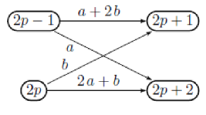
The benchmarks of the minimisation of “Railroad” automata are shown on Table 2. On these automata, if a temporary class contains all states between and , it is split into one class and one class : the size of the classes lowers slowly. On these examples, DSA and PCSA are therefore quadratic.
| DSA | (s) | 3.29 | 53.2 | 214 | _ | ||
|---|---|---|---|---|---|---|---|
| / | 3.1 | 3.2 | 3.2 | ||||
| PCSA | (s) | 0.31 | 4.92 | 20.5 | 86.1 | 346 | _ |
| / | 3.0 | 2.9 | 3.1 | 3.2 | 3.2 | ||
| FPCSA | (s) | 0.12 | 0.24 | 30.8 | |||
| / | 7.8 | 7.3 | 7.4 | 7.3 | 7.3 | 7.3 | |
In FPCSA, when this splitting occur, the largest class () is not put in the queue for further splittings; therefore, except at the first round, all splitters are pairs of states and the algorithm is linear.
References
- [1] Hopcroft JE, Motwani R, Ullman JD. Introduction to Automata Theory, Languages and Computation. Addison-Wesley, 2006. 3rd edition. ISBN-10:0321455363, 13:978-0321455369.
- [2] Pin JÉ (ed.). Handbook of Automata Theory. EMS Press, 2021. ISBN-978-3-98547-006-8.
- [3] Berstel J, Boasson L, Carton O, Fagnot I. Minimisation of Automata. In: Pin JÉ (ed.), Handbook of Automata Theory, Vol. I, pp. 337–373. EMS Press, 2021. doi:10.48550/arXiv.2008.06790.
- [4] Droste M, Kuich W, Vogler H (eds.). Handbook of Weighted Automata. Springer, 2009. doi:10.1007/978-3-642-01492-5.
- [5] Garey MR, Johnson DS. Computers and Intractability: A Guide to the Theory of NP-Completeness (Series of Books in the Mathematical Sciences). W. H. Freeman, 1979. ISBN-10:0716710455, 13:978-0716710455.
- [6] Baier C, Hermanns H. Weak Bisimulation for Fully Probabilistic Processes. In: Grumberg O (ed.), CAV 1997, volume 1254 of Lect. Notes in Comput. Sci. Springer, 1997 pp. 119–130. doi:10.1007/3-540-63166-6_14.
- [7] Boreale M. Weighted Bisimulation in Linear Algebraic Form. In: Bravetti M, Zavattaro G (eds.), CONCUR 2009, volume 5710 of Lect. Notes in Comput. Sci. Springer, 2009 pp. 163–177. doi:10.1007/978-3-642-04081-8_12.
- [8] Awali: Another Weighted Automata LIbrary. vaucanson-project.org/Awali.
- [9] Lombardy S, Sakarovitch J. Two Routes to Automata Minimization and the Ways to Reach It Efficiently. In: Câmpeanu C (ed.), CIAA 2018, volume 10977 of Lect. Notes in Comput. Sci. Springer, 2018 pp. 248–260. doi:10.1007/978-3-319-94812-6_21.
-
[10]
Sakarovitch J.
Elements of Automata Theory.
Cambridge University Press, 2009.
doi:10.1017/
CBO9781139195218. - [11] Frougny C, Sakarovitch J. Synchronized relations of finite and infinite words. Theoretical Computer Science, 1993. 108:45–82.
- [12] Reutenauer C. Subsequential functions: characterizations, minimization, examples. In: IMYCS’90, number 464 in Lect. Notes in Comput. Sci. 1990 pp. 62–79.
- [13] Béal MP, Lombardy S, Sakarovitch J. Conjugacy and Equivalence of Weighted Automata and Functional Transducers. In: Grigoriev D (ed.), CSR 2006, number 3967 in Lect. Notes in Comput. Sci. 2006 pp. 58–69. doi:10.1007/11753728_9.
- [14] Lind D, Marcus B. An Introduction to Symbolic Dynamics and Coding. Cambridge University Press, 1995. doi:10.1017/CBO9780511626302.
- [15] Milner R. A Complete Axiomatisation for Observational Congruence of Finite-State Behaviors. Inf. Comput., 1989. 81(2):227–247.
- [16] Benson DB, Ben-Shachar O. Bisimulation of Automata. Inf. Comput., 1988. 79(1):60–83.
- [17] Larsen KG, Skou A. Bisimulation through Probabilistic Testing. Inf. Comput., 1991. 94(1):1–28. doi: 10.1016/0890-5401(91)90030-6.
- [18] Lombardy S, Sakarovitch J. Derived terms without derivation. J. Comput. Sci. and Cybernetics, 2021. 37(3):201–221. In arXiv: arxiv.org/abs/2110.09181.
- [19] Béal MP, Crochemore M. Minimizing incomplete automata. In: Finite-State Methods and Natural Language Processing FSMNLP’08. 2008 pp. 9–16. ISBN-9781586039752.
- [20] Moore EF. Gedanken-Experiments on Sequential Machines. In: Shannon C, McCarthy J (eds.), Automata Studies, pp. 129–153. Princeton University Press, 1956. doi:10.1515/9781400882618-006.
- [21] Paige R. Efficient Translation of External Input in a Dynamically Typed Language. In: Technology and Foundations - Information Processing IFIP’94, volume A-51 of IFIP Transactions. North-Holland, 1994 pp. 603–608. ID:9443428.
- [22] Cormen TH, Leiserson CE, Rivest RL, Stein C. Introduction to Algorithms, 3rd Edition. MIT Press, 2009. ISBN-978-0-262-03384-8. URL http://mitpress.mit.edu/books/introduction-algorithms.
- [23] Knuth DE. The Art of Computer Programming, Volume III, Sorting and Searching, 2nd Edition. Addison-Wesley, 1998. ISBN-0201896850. URL https://www.worldcat.org/oclc/312994415.
-
[24]
JavaTM Platform.
Standard Edition 17 API Specification. Class
LinkedHashMap<K,V>, 2021. Available at: https://docs.oracle.com/en/java/javase/17/docs/api/java.base/java/util/LinkedHashMap.html. -
[25]
Gries D.
Describing an algorithm by Hopcroft.
Acta Informatica, 1973.
2:97–109. doi:10.1007/
BF00264025. - [26] Berstel J, Carton O. On the Complexity of Hopcroft’s State Minimization Algorithm. In: Implementation and Application of Automata CIAA’04, volume 3317 of Lect. Notes in Comput. Sci. Springer, 2004 pp. 35–44. doi:10.1007/978-3-540-30500-2_4.
- [27] Valmari A, Lehtinen P. Efficient Minimization of DFAs with Partial Transition. In: STACS’08, volume 1 of LIPIcs. Schloss Dagstuhl, 2008 pp. 645–656. doi:10.4230/LIPIcs.STACS.2008.1328.
- [28] Hopcroft JE. An Algorithm for Minimizing States in a Finite Automaton. In: Kohavi Z, Paz A (eds.), Theory of Machines and Computations, pp. 189–196. Academic Press, New York, 1971. doi:10.1016/B978-0-12-417750-5.50022-1.
- [29] Paige R, Tarjan RE. Three Partition Refinement Algorithms. SIAM J. Comput., 1987. 16(6):973–989. doi:10.1137/0216062.
- [30] Fernandez JC. An Implementation of an Efficient Algorithm for Bisimulation Equivalence. Sci. Comput. Program., 1989. 13(1):219–236. 10.1016/0167-6423(90)90071-K.
- [31] Castiglione G, Restivo A, Sciortino M. On extremal cases of Hopcroft’s algorithm. Theor. Comput. Sci., 2010. 411(38-39):3414–3422. doi:10.1016/j.tcs.2010.05.025.