Cluster cosmology with anisotropic boosts: Validation of a novel forward modeling analysis and application on SDSS redMaPPer clusters

Abstract

We present a novel analysis for cluster cosmology that fully forward models the abundances, weak lensing, and the clustering of galaxy clusters. Our analysis notably includes an empirical model for the anisotropic boosts impacting the lensing and clustering signals of optical clusters. These boosts arise from a preferential selection of clusters surrounded by anisotropic large scale structure, a consequence of the limited discrimination between line-of-sight interlopers and true cluster members offered by photometric surveys. We validate our analysis via a blind cosmology challenge on mocks, and find that we can obtain tight and unbiased cosmological constraints without informative priors or external calibrations on any of our model parameters. We then apply our analysis on the SDSS redMaPPer clusters, and find results favoring low $\Omega_{\mathrm{m}}$ and high $\sigma_{8}$, combining to yield the lensing strength constraint $S_{8}=0.715_{-0.021}^{+0.024}$. We investigate potential drivers behind these results through a series of post-unblinding tests, noting that our results are consistent with existing cluster cosmology constraints but clearly inconsistent with other CMB/LSS based cosmology results. From these tests, we find hints that a suppression in the cluster lensing signal may be driving our results.

1 Introduction

Galaxy clusters have long been promised to become exquisite probes for the cosmic growth of structure and the accelerated expansion of the Universe (Vikhlinin et al., 2009; Rozo et al., 2010; Allen et al., 2011; Weinberg et al., 2013; Huterer et al., 2015; Dodelson et al., 2016). As tracers of the highest peaks in the primordial matter density fluctuations, and the most massive halos in the Universe born therefrom (Bardeen et al., 1986; Kravtsov & Borgani, 2012), clusters probe the high-mass end of the halo mass function, exponentially sensitive to cosmological parameters (Haiman et al., 2001; Lima & Hu, 2005). The caveat underlying this sensitivity, however, has always been the calibration of cluster masses. Mass calibrations connect the theoretical predictions for cluster-sized halos to the catalogs of observed clusters in real data, and the precision and accuracy of these calibrations limit the quality of cosmological constraints achievable via cluster studies.

This has made optically identified clusters from photometric surveys a sample of particular interest. Photometric surveys allow for uniform and complete observations of clusters (Rykoff et al., 2014; Rozo & Rykoff, 2014; Rozo et al., 2015a, b; Oguri, 2014), and at the same time detect weak lensing signals around clusters by observing the shapes of galaxies residing in the background of clusters. By combining the observed cluster abundances with the halo mass information afforded by the cluster lensing signal (Johnston et al., 2007; von der Linden et al., 2014; Mantz et al., 2015; Simet et al., 2017; Murata et al., 2018; McClintock et al., 2019; Murata et al., 2019), a self-contained analysis that constrains cosmology and calibrates cluster masses becomes possible (Lima & Hu, 2005; Takada & Bridle, 2007; Rozo et al., 2010; Oguri & Takada, 2011). The most recent incarnations of this joint cluster cosmology analysis are Costanzi et al. (2019) and DES Collaboration et al. (2020). These studies calibrated cluster masses using cluster lensing signals, then used the calibrations to simultaneously constrain the cosmology and the mass-observable relation (MOR) using cluster abundances. Interestingly, both results (in particular the latter) found that the resulting cosmological constraints favored lower $\Omega_{\mathrm{m}}$ and higher $\sigma_{8}$ compared against other constraints derived from cosmic microwave background (CMB) or large scale structure (LSS) data. These findings hinted at yet unknown systematic effects, or new physics, surrounding optical clusters.

Simultaneously with these results, we showed in Sunayama et al. (2020) (SP20 henceforth) that the interaction between optical cluster finding algorithms and the weaker line-of-sight resolution of photometric surveys resulted in observed cluster samples with a characteristic anisotropy in the LSS around them. Briefly, SP20 populated galaxies into halos from N-body simulations following an HOD prescription, ran a mock cluster finder algorithm on these galaxies to generate catalogs of mock observed clusters, and studied the lensing and clustering signals exhibited by these mock clusters. From these studies, SP20 found that optically identified clusters were likely to be embedded in LSS elongated along the line-of-sight, e.g., filaments aligned with the line-of-sight, and importantly that this anisotropy led to large-scale boosts of the cluster lensing and cluster clustering signals (also see Osato et al., 2018, for a similar discussion). These anisotropic boosts, which have now been observationally confirmed by To et al. (2021), have significant implications for the joint cluster cosmology framework, as they break the isotropic halo model generally assumed in making lensing mass calibrations for clusters. If not properly modeled, these anisotropic boosts inevitably leads to errors in the cluster mass calibrations.

Thus, the natural continuation of these findings from SP20 is to build a novel analysis framework that accounts for the anisotropic boosts in the cluster lensing and cluster clustering signals, and the main goal of this paper is to achieve exactly that. Namely, in this work we build an analysis framework combining cluster abundances, lensing, and clustering, and introduce an explicit model for the anisotropic boosts. We focus on two major research questions:

1. Can we obtain unbiased and competitive cosmological constraints from clusters with freely varied systematics models, in particular for the anisotropic boost?

2. If we can validate this approach, what results do we find when we perform the analysis on real data and how do they compare against existing results?

Let us elaborate further on these two questions. In (i), we are interested in studying the cosmological information content in cluster observables as agnostically as possible, i.e., without informative priors or simulation-based calibrations. We achieve this by using flat uninformative priors for all of our model parameters, making the functional forms of our modeling ingredients the only externally informed elements of our analysis. This approach is complementary to those from Costanzi et al. (2019) and DES Collaboration et al. (2020), which involve multiple informative priors and calibrations. As for (ii), we are mainly interested in whether the explicit modeling of anisotropic boosts leads to different cosmological conclusions from existing cluster cosmology results. DES Collaboration et al. (2020) argued that their results are most likely impacted by a suppression in the lensing signals of low-richness clusters, which is the opposite of effects that anisotropic boosts would produce. At the same time, it is unclear whether this suppression is limited to the particular choice of data set and modeling, or it globally affects cluster cosmology analyses. We seek to answer this question with a completely independent combination of data and modeling approach.

This paper is structured as follows. In Section 2, we describe the theoretical model we employ, including emulator-based halo model predictions and models for common cluster systematics as well as for anisotropic boosts. In Section 3, we discuss tests of this model on unblinded mocks and the subsequent validation of our fiducial analysis via a blind cosmology challenge on an independent set of mocks. We then discuss the blind application of our analysis pipeline on real data in Section 4, and present a series of post-unblinding tests in Section 5. We finally summarize our work and discuss its implications in Section 6.

2 Modeling

2.1 Emulator predictions

Throughout this paper, we use the Dark Emulator (Nishimichi et al., 2019, darkemu  henceforth) software to generate base predictions for halo model quantities. Specifically, for a given set of cosmological parameters $\bm{\uptheta}$ and redshift $z$ there are three fundamental quantities that we obtain from darkemu:

• The halo mass function $\mathrm{d}n/\mathrm{d}\ln M$

• The 3D halo-matter correlation function $\xi_{\mathrm{hm}}(r|M)$

• The 3D halo-halo correlation function $\xi_{\mathrm{hh}}(r|M,M^{\prime})$

with halo masses $M$ and $M^{\prime}$. Note that we suppress the $\bm{\uptheta}$ and $z$ dependence of quantities in our notation throughout. The emulator was trained based on the measurement of the above quantities in a suite of 101 numerical simulations that were run to optimally span a 6-parameter space of cosmological models. The accuracy of the emulation was tested with a set of test simulations that also spanned the parameter space and were reserved during the training process. The emulator is accurate to 2% in the predictions of halo-matter correlation functions relevant for galaxy-galaxy lensing, and to 4% in the predictions of halo autocorrelation functions relevant for the estimates of clustering, in the range of its validity ($0<z<1.48$ and $M\gtrsim 10^{12}h^{-1}M_{\odot}$). The darkemu code then analytically converts the 3D statistics to the projected 2D statistics, which are the main focus of the current investigation. The emulation accuracy was also tested for the projected lensing and clustering statistics, using mock galaxy catalogs roughly corresponding to the BOSS CMASS galaxy sample (Dawson et al., 2013). It was confirmed that the projected statistics from the emulator agreed with measurements from the mock galaxy catalogs at the same level as the original 3D statistics. In using the emulator to calculate our model predictions, we assume a flat $\Lambda$CDM model of cosmology with the neutrino density fixed to $\Omega_{\nu}h^{2}=0.00064$, and ignore the redshift evolution of the halo statistics by calculating these quantities at a single representative redshift. We also adopt the “$200m$” halo definition throughout, following the darkemu conventions.

We then map these quantities to cluster observables as follows. First, for cluster abundances in a given richness bin, we have

$$N_{\mathrm{c},i} = \Omega\int\!\mathrm{d}z~{}\frac{\mathrm{d}^{2}V}{\mathrm{d}z\mathrm{d}\Omega}\int_{\ln\lambda_{\mathrm{i,min}}}^{\ln\lambda_{\mathrm{i,max}}}\!\mathrm{d}\ln\lambda\int\!\mathrm{d}\ln M\frac{\mathrm{d}n}{\mathrm{d}\ln M}P(\ln\lambda|M)$$ (1)

$$= \Omega\int\!\mathrm{d}z\frac{\chi^{2}(z)}{H(z)}\int\!\mathrm{d}\ln M\frac{\mathrm{d}n}{\mathrm{d}\ln M}S_{i}(M),$$

with richness $\lambda$, the effective survey area $\Omega$, comoving distance $\chi$, and the Hubble constant $H$. We follow Murata et al. (2018) to define our mass-richness relation $P(\ln\lambda|M)$ as a log-normal distribution, i.e. $\ln\lambda\sim\mathcal{N}(\mu_{\mathrm{M}},\sigma_{\mathrm{M}}^{2})$, with mean $\mu_{\mathrm{M}}$ and standard deviation $\sigma_{\mathrm{M}}$ given by

$$\mu_{\mathrm{M}} = A+B\ln\left(\frac{M}{M_{\mathrm{piv}}}\right),$$ (2)

$$\sigma_{\mathrm{M}} = \sigma_{0}+q\ln\left(\frac{M}{M_{\mathrm{piv}}}\right).$$ (3)

We set our pivot mass $M_{\mathrm{piv}}=3\times 10^{14}M_{\odot}/h$. This then gives the following mass selection function $S_{i}(M)$,

$$S_{i}(M) = \int_{\ln\lambda_{\mathrm{i,min}}}^{\ln\lambda_{\mathrm{i,max}}}d\ln\lambda~{}P(\ln\lambda|M)$$ (4)

$$= \Phi(\ln\lambda_{\mathrm{i,max}}|\mu_{\mathrm{M}},\sigma_{\mathrm{M}})-\Phi(\ln\lambda_{\mathrm{i,min}}|\mu_{\mathrm{M}},\sigma_{\mathrm{M}}),$$

where $\Phi(x|\mu,\sigma)$ is the cumulative distribution function of a Gaussian distribution with mean $\mu$ and standard deviation $\sigma$:

$$\Phi(x|\mu,\sigma)=\frac{1}{2}\left[1+\mathrm{erf}\left(\frac{x-\mu}{\sqrt{2}\sigma}\right)\right],$$ (5)

with $\mathrm{erf}(x)$ being the error function.

Next, we model the cluster lensing signal as follows. We first obtain the cluster-matter correlation function for the $i$-th bin as

$$\xi_{\mathrm{cm},i}(r)=\frac{1}{n_{\mathrm{c},i}}\int\!\mathrm{d}\ln M~{}\frac{\mathrm{d}n}{\mathrm{d}\ln M}S_{i}(M)\xi_{\mathrm{hm}}(r|M),$$ (6)

with the cluster number density for the $i$-th bin $n_{\mathrm{c},i}$ given by

$$n_{\mathrm{c},i}=\int\!\mathrm{d}\ln M~{}\frac{\mathrm{d}n}{\mathrm{d}\ln M}S_{i}(M).$$ (7)

We then obtain the surface density of matter around clusters $\Sigma(R)$ as

$$\Sigma_{i}(R)=\bar{\rho}_{\mathrm{m},0}\int_{-\infty}^{\infty}\!\mathrm{d}\pi~{}\xi_{\mathrm{cm},i}\left(\sqrt{R^{2}+\pi^{2}}\right),$$ (8)

where we only consider the matter density in the Universe that contributes to lensing. Here, $R$ is the separation perpendicular to the line-of-sight, and $\pi$ is the separation parallel. We finally obtain the cluster lensing observable, i.e., the excess surface density $\Delta\Sigma(R)$, with the usual formalism

$$\Delta\Sigma_{i}(R) \equiv \left<\Sigma_{i}\right>(<R)-\Sigma_{i}(R)$$ (9)

$$= \frac{2}{R^{2}}\int_{0}^{R}\mathrm{d}R^{\prime}R^{\prime}\Sigma_{i}(R^{\prime})-\Sigma_{i}(R).$$

Equivalently, $\Delta\Sigma(R)$ is given by

$$\Delta\Sigma(R) = \bar{\rho}_{\mathrm{m},0}\int\!\frac{KdK}{2\pi}J_{2}(KR)C_{\mathrm{cm}}(K)$$ (10)

$$\simeq \bar{\rho}_{\mathrm{m},0}\int\!\frac{kdk}{2\pi}J_{2}(kR)P_{\mathrm{cm}}(k),$$ (11)

where $C_{\mathrm{cm}}(K)$ and $P_{\mathrm{cm}}(k)$ are the 2D and 3D cluster-matter power spectra with the 2D wavenumber $K$ and the 3D wavenumber $k$, and $J_{2}$ is the second-order Bessel function. The last line uses the the Limber approximation (Limber, 1954; Kaiser, 1992), which becomes exact under our assumption of a single redshift value (also see Hikage et al., 2013; Miyatake et al., 2021).

Lastly, we model the cluster clustering signal. Similar to the lensing case, we first derive the cluster autocorrelation function for the $i$-th bin as

$$\begin{split}\xi_{\mathrm{cc},i}(r)=\frac{1}{(n_{\mathrm{c},i})^{2}}\int\!\mathrm{d}M\int\!\mathrm{d}M^{\prime}~{}&\frac{\mathrm{d}n}{\mathrm{d}\ln M}\frac{\mathrm{d}n}{\mathrm{d}\ln M^{\prime}}~{}\times\\ &S_{i}(M)S_{i}(M^{\prime})\xi_{\mathrm{hh}}(r|M,M^{\prime}).\end{split}$$ (12)

We then model the cluster clustering observable, i.e., the projected cluster autocorrelation function $w_{\mathrm{p}}(R)$, as

$$w_{\mathrm{p}}(R)=\int_{-\pi_{\mathrm{max}}}^{\pi_{\mathrm{max}}}\!\mathrm{d}\pi~{}\xi_{\mathrm{cc},i}\left(\sqrt{R^{2}+\pi^{2}}\right),$$ (13)

where $\pi_{\mathrm{max}}$ is the maximum line-of-sight projection width. We decide to use $\pi_{\rm max}=100\,h^{-1}{\rm Mpc}$ as our fiducial choice after tests in Section 3.1.

2.2 Anisotropic boosts

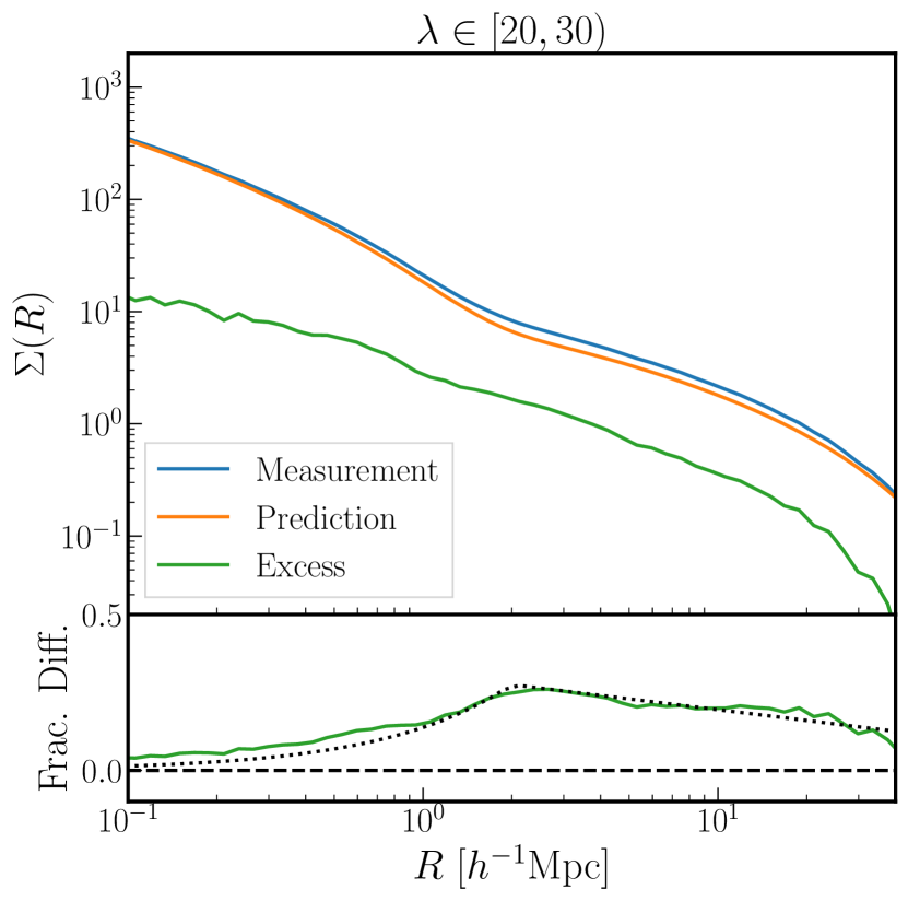
Figure 1: The surface density profiles related to the mock observed clusters from SP20 simulations. Top: the measured surface density (blue) shows an excess (green) when compared against emulator predictions corresponding to the underlying masses (orange). Bottom: the excess is shown as a fraction of the emulator prediction. A rough fit using the model in Equation 16 (dotted line) is also shown to guide the eye.

Our analysis explicitly accounts for the anisotropic boosts on the cluster lensing and cluster clustering signals, reflecting the following insights we first discussed in SP20:

• The LSS around optically identified clusters is not isotropic. Rather, some optical clusters are likely to be embedded within anisotropic LSS, e.g., filaments that are aligned with the line-of-sight.

• The most salient impact of the anisotropic LSS is a boost on the large-scale regimes of the cluster lensing and cluster clustering signals.

• The respective multiplicative boosts for the lensing and clustering signals show a consistent factor-of-two relation, with the latter being twice as big as the former. This suggests that modifications to the cluster bias may consistently explain both boosts.

Drawing on these insights, we model the boost induced by the anisotropic LSS as a scale-dependent multiplicative factor $\Pi(R)$ applied on the cluster bias. This then transforms the isotropic predictions from Section 2.1 as

$$\Sigma(R) = \Pi(R)\Sigma^{\mathrm{iso}}(R),$$ (14)

$$w_{\mathrm{p}}(R) = \Pi^{2}(R)w_{\mathrm{p}}^{\mathrm{iso}}(R).$$ (15)

Note that while $\Pi(R)$ directly modifies the observable $w_{\mathrm{p}}(R)$ on the clustering side, it acts on the underlying physical quantity $\Sigma(R)$ rather than the direct observable $\Delta\Sigma(R)$ on the lensing side. This is because $\Sigma(R)$ is the quantity that represents the raw cluster-matter correlation function; by modifying $\Sigma(R)$, we maintain our interpretation of $\Pi(R)$ as an effective modification of the scale-dependent cluster bias.

We then empirically design a functional form for the projection factor $\Pi(R)$. To do so, we go back to the results from SP20 and examine the measured surface density profiles for mock clusters. In Figure 1, we show an example from those results. From the fractional differences between the isotropic prediction and the mock results in the bottom panel, we see that the anisotropic boost shows two distinct regimes. On small scales, the boost is roughly linear in $R$ (exponential in $\ln R$) up to a turnover separation of a few Mpc$/h$. After the turnover, the boost slowly falls off logarithmically. Thus, we model $\Pi(R)$ as a piecewise function:

$$\Pi(R)=\begin{cases}\Pi_{0}(R/R_{0})&\text{for }R\leq R_{0},\\ \Pi_{0}+c\ln(R/R_{0})&\text{for }R>R_{0}.\end{cases}$$ (16)

The boost model is given by three model parameters, $\Pi_{0},R_{0}$ and $c$. The parameters $\Pi_{0}$ and $R_{0}$ are defined for each richness bin, while $c$ is shared across all richness bins. We show a rough fit using this functional form in the bottom panel of Figure 1 to guide the eye.

2.3 Miscentering

Operationally, cluster centers are defined by the location of the brightest cluster galaxy (BCG) within each cluster. This, however, does not always match with the true center of the dark matter halo hosting the cluster (Oguri & Takada, 2011; Hikage et al., 2013; Miyatake et al., 2016). When this mismatch happens, the cluster lensing signal measured around the BCG will receive a characteristic dilution on small scales. To model this dilution, we assume that a fraction ($f_{\mathrm{mis}}$) of clusters are miscentered by a random variable $R^{\prime}$ that follows the Rayleigh distribution

$$P_{\mathrm{mis}}(R^{\prime}|R_{\mathrm{mis}})=\frac{R^{\prime}}{R_{\mathrm{mis}}^{2}}\exp\left(-\frac{R^{\prime 2}}{2R_{\mathrm{mis}}^{2}}\right).$$ (17)

As shown by Oguri & Takada (2011), this assumption nicely simplifies the calculation of the averaged lensing profile for the miscentered population in Fourier space:

$$C_{\mathrm{cm}}^{\mathrm{mis}}(K) = C_{\mathrm{cm}}(K)\int\!\mathrm{d}R^{\prime}J_{0}(KR^{\prime})P_{\mathrm{mis}}(R^{\prime}|R_{\mathrm{mis}})$$ (18)

$$= C_{\mathrm{cm}}(K)\exp\left(-\frac{1}{2}K^{2}R_{\mathrm{mis}}^{2}\right).$$

The global average is then given by

$$C_{\mathrm{cm}}^{\mathrm{tot}}(K)=(1-f_{\mathrm{mis}})C_{\mathrm{cm}}(K)+f_{\mathrm{mis}}C_{\mathrm{cm}}^{\mathrm{mis}}(K),$$ (19)

which can be Fourier transformed back to real space to yield the cluster lensing signal with miscentering accounted for.

2.4 Cluster photo-$z$ scatter

The photometric redshifts of clusters are generally better characterized than galaxies, but the scatter in the estimated redshifts still produce non-negligible dilutions in cluster clustering measurements. To model this effect, we assume a Gaussian scatter in the inferred line-of-sight positions of clusters, characterized by the standard deviation $\sigma_{\mathrm{ph}}$. This scatter is then taken into account in the calculation of the cluster autocorrelation function $w_{\mathrm{p}}(R)$ as a modification to Equation 13,

$$w_{\mathrm{p}}(R)=2\int_{0}^{\infty}\!\mathrm{d}\pi~{}S_{\mathrm{ph}}(\pi|\pi_{\mathrm{max}},\sigma_{\mathrm{ph}})~{}\xi_{\mathrm{cc},i}\left(\sqrt{R^{2}+\pi^{2}}\right),$$ (20)

where the line-of-sight separation selection function $S_{\mathrm{ph}}(\pi,\sigma_{\mathrm{ph}})$ is given by

$$S_{\mathrm{ph}}(\pi|\pi_{\mathrm{max}},\sigma_{\mathrm{ph}})=\Phi(\pi|-\pi_{\mathrm{max}},\sqrt{2}\sigma_{\mathrm{ph}})-\Phi(\pi|\pi_{\mathrm{max}},\sqrt{2}\sigma_{\mathrm{ph}})$$ (21)

with $\Phi(x|\mu,\sigma)$ being the cumulative distribution function for a Gaussian distribution with mean $\mu$ and standard deviation $\sigma$.

Note that we do not consider the impact of photo-$z$ scatter for abundances and lensing. For abundances, as our model does not have a redshift dependent richness-mass relation, the effect of photo-$z$ scatter is essentially a smoothing of the redshift boundaries as we integrate over the entire redshift range. We estimate this effect to be very small – less than 0.2% assuming a Planck cosmology and typical cluster photo-$z$ errors. For lensing, photo-$z$ scatter will confound the estimated critical surface density values used to translate tangential shear measurements to $\Delta\Sigma$. We estimate this effect to be less than 0.4%, also very small.

2.5 Parameter inference

Throughout this work, we assume a Gaussian likelihood

$$\ln P(\mathbf{d}|\bm{\uptheta})=-\frac{1}{2}\left[\mathbf{d}-\bm{\upmu}(\bm{\uptheta})\right]^{\intercal}\mathbf{C}^{-1}\left[\mathbf{d}-\bm{\upmu}(\bm{\uptheta})\right]$$ (22)

with measurements $\mathbf{d}$, parameters $\bm{\uptheta}$, model predictions $\bm{\upmu}(\bm{\uptheta})$, and covariances $\mathbf{C}$. Based on this likelihood, we perform Bayesian parameter inferences for the posterior $P(\bm{\uptheta}|\mathbf{d})$ as

$$P(\bm{\uptheta}|\mathbf{d})\propto P(\mathbf{d}|\bm{\uptheta})P(\bm{\uptheta}),$$ (23)

with our likelihood $P(\mathbf{d}|\bm{\uptheta})$ and prior $P(\bm{\uptheta})$. We perform our likelihood analysis with the cosmosis (Zuntz et al., 2015) software, using the polychord (Handley et al., 2015a, b) and the multinest (Feroz & Hobson, 2008; Feroz et al., 2009; Feroz et al., 2019) samplers integrated therein to sample our posteriors. We also use the chainconsumer (Hinton, 2016) software to plot confidence regions for our posterior samples. Under the fiducial analysis setup we describe further in Section 3.1, we end up with a total of 27 independently varied model parameters: 5 for cosmology, 4 for MOR, 9 for anisotropic boosts, 8 for miscentering, and 1 for the cluster photo-$z$ scatter.

3 Tests and Validation

3.1 Model tests on SP20 mocks

We first test our model in Section 2 using the unblinded mock cluster catalogs and measurements from SP20. Briefly, these mock catalogs start with N-body simulations and resulting halo catalogs from Nishimichi et al. (2019). Identified halos with masses greater than $10^{12}M_{\odot}/h$ are then populated with galaxies, following an HOD prescription for the number of galaxies populated and a Navarro-Frenk-White (NFW; Navarro et al., 1997) profile for the spatial distribution of populated galaxies. Finally, a cluster finder algorithm based on Sunayama & More (2019) is run on the galaxy catalog, yielding the catalog of mock-observed clusters. We use a total of 19 realizations of this mock catalog, each with $1~{}(\mathrm{Gpc}/h)^{3}$ volume and all at redshift $z=0.251$ to emulate the SDSS redMaPPer catalog, and additionally 14 realizations of $2~{}(\mathrm{Gpc}/h)^{3}$ volume snapshots for better statistics on the cluster clustering measurements. For more details on the test simulations, as well as the measurement procedures we use on the mock catalogs, we refer the reader to Sections 2.2 – 2.5 of SP20.

Table 1: The model parameters varied in our fiducial analysis and the respective priors assumed.

Parameter	Prior
Cosmological parameters
$\Omega_{\mathrm{b}}h^{2}$	$\mathcal{U}(0.0211375,0.0233625)$
$\Omega_{\mathrm{c}}h^{2}$	$\mathcal{U}(0.10782,0.13178)$
$\ln 10^{10}A_{\mathrm{s}}$	$\mathcal{U}(2.5,3.7)$
$n_{\mathrm{s}}$	$\mathcal{U}(0.92,1.01)$
$\Omega_{\Lambda}$	$\mathcal{U}(0.54752,0.82128)$
Mass-richness relation
$A$	$\mathcal{U}(0.5,5.0)$
$B$	$\mathcal{U}(0.0,2.0)$
$\sigma_{0}$	$\mathcal{U}(0.0,1.5)$
$q$	$\mathcal{U}(-1.5,1.5)$
Anisotropic boost parameters
$\Pi_{\mathrm{0,1-4}}$	$\mathcal{U}(0.0,1.0)$
$R_{\mathrm{0,1-4}}$	$\mathcal{U}(0.1,5.0)$
$c$	$\mathcal{U}(-2.0,2.0)$
Miscentering
$f_{\mathrm{mis,1-4}}$	$\mathcal{U}(0.0,1.0)$
$R_{\mathrm{mis,1-4}}$	$\mathcal{U}(0.0,1.0)$
Cluster photo-$z$ scatter
$\sigma_{\mathrm{ph}}$	$\mathcal{U}(1.0,100.0)$

Our goal in this step is to use these unblinded mock catalogs to identify the optimal form of the analysis. We begin by fixing the basic format of our data vector. The mock catalog is divided into four richness bins, respectively defined as $\lambda\in[20,30),[30,40),[40,55),$ and $[55,200)$. Our data vector is then given by

$$\mathbf{d}=\left\{\mathbf{N}_{\mathrm{c}},\bm{\upDelta\upSigma}_{1},\bm{\upDelta\upSigma}_{2},\bm{\upDelta\upSigma}_{3},\bm{\upDelta\upSigma}_{4},\mathbf{w}_{\mathrm{p,1}},\mathbf{w}_{\mathrm{p,2}},\mathbf{w}_{\mathrm{p,3}},\mathbf{w}_{\mathrm{p,4}}\right\},$$ (24)

where $\bm{\upDelta\upSigma}_{i}$ and $\mathbf{w}_{\mathrm{p,i}}$ respectively represent the cluster lensing and cluster clustering signals for the $i$-th richness bin, and $\mathbf{N}_{\mathrm{c}}=\{N_{\mathrm{c,i}}\}$ is the vector of cluster counts for the four richness bins. Since the original measurements in SP20 assume perfect knowledge of cluster positions, in this work we add more reality to these measurements by introducing miscentering and photo-$z$ errors. For miscentering, we randomly displace the cluster centers in the 2D plane perpendicular to the line-of-sight, following the same model in Section 2.3. For photo-$z$ errors, we again randomly displace the cluster centers but now in the line-of-sight direction, following a Gaussian distribution.

Starting from this setup, we test a number of analysis choices including:

• Range and binning of radial scales to be used for analysis,

• The line-of-sight projection width ($\pi_{\mathrm{max}}$) for $w_{\mathrm{p}}$,

• Functional form of the effective bias $\Pi(R)$ modeling the anisotropic boosts on lensing and clustering observables,

• Dependence on priors and parameter space volumes.

Each test takes the form of a likelihood analysis, and our key concern is the robust recovery of the cosmological parameters $\Omega_{\mathrm{m}}$ and $\sigma_{8}$, and their combination $S_{8}=\sigma_{8}(\Omega_{\mathrm{m}}/0.3)^{0.5}$. These parameters are derived from the five input cosmological parameters for darkemu ($\Omega_{\mathrm{b}}h^{2}$, $\Omega_{\mathrm{c}}h^{2}$, $\ln 10^{10}A_{\mathrm{s}}$, $n_{\mathrm{s}}$, and $\Omega_{\Lambda}$) that we directly vary. As mentioned above, there are three versions of measurements that we consider: nomis-test, the original SP20 measurements without miscentering or photo-$z$ scatter; mis-test, the version with miscentering included; and photo-test, the version with miscentering and photo-$z$ scatter included. Each version of measurement is then analyzed with a corresponding model, i.e., a model that takes into account the set of systematic effects included. We use covariances estimated directly from the SDSS redMaPPer catalog, version 6.3, via jackknife resampling. The resampling uses 83 independent jackknife regions, and we assume a block-diagonal covariance matrix where each of the 9 components of our data vector are considered uncorrelated. This approximation was shown to be reasonable in previous studies (e.g., Simet et al., 2017), and we also find that the off-block-diagonal components of the full covariance matrix are negligible, in part due to the domination of shape noise in the cluster lensing covariances.

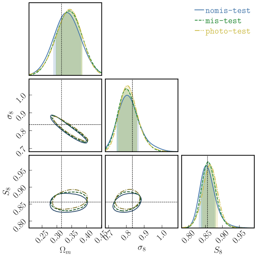
Figure 2: The 68% confidence regions for cosmological parameters of interest, obtained by running our fiducial pipeline on the test mocks. Blue contours assume no systematics, green assumes the existence of miscentering, and yellow assumes the existence of both miscentering and cluster photo-$z$ scatter. Dashed lines represent the input cosmology for the mocks.

Based on these tests, we define our lensing data vector with 12 logarithmically spaced bins spanning $R\in[0.2,50]$ Mpc/$h$, and our clustering data vector with 6 logarithmically spaced bins spanning $R\in[2,50]$ Mpc/$h$. For the clustering side, we set $\pi_{\mathrm{max}}=100$ Mpc/$h$ as our fiducial line-of-sight projection width for $w_{\mathrm{p}}$. Under these analysis choices, we confirm that our anisotropic boost model for $\Pi(R)$ presented in Section 2.2 yields robust results, with the recovered amplitudes of the anisotropic boosts agreeing well with the values we found in SP20. We also find that for the mis-test and the photo-test cases our respective constraints on the miscentering and photo-$z$ scatter parameters are in good agreement with the input values. Finally, we find that we recover tight cosmological constraints without significant parameter space volume effects despite the broad, uninformative priors we assume for all model parameters, as detailed in Table 1. In Figure 2, we show the test results under this fiducial setup. For these results, as well as for the validation results presented in Section 3.2, we use the multinest sampler. For all three versions of the measurements, we recover the input cosmology well within the 1-$\sigma$ confidence region in the $\Omega_{\mathrm{m}}$-$S_{8}$ plane. Our fiducial model and analysis choices are frozen at this point.

3.2 Validation

With the model and analysis setup successfully developed in Section 3.1, we move to a blind validation of our model. In this step, an entirely new set of mock cluster catalogs is generated. The new mocks are different from the original SP20 mocks starting from the N-body level; instead of 1 $(\mathrm{Gpc}/h)^{3}$ snapshots with $2048^{3}$ particles, we use 5 independent realizations with 2.5 $(\mathrm{Gpc}/h)^{3}$ volumes and $3000^{3}$ particles, generated with a newly developed TreePM code (T. Nishimichi, S. Tanaka and K. Yoshikawa, in prep). Due to the larger volumes of these new realizations, the mass resolution slightly decreases, which leads to less interloper contamination for detected clusters and thus slightly weaker anisotropic boosts overall. The underlying cosmological parameters are also meaningfully different from SP20. In addition, two different miscentering models are used on the mock clusters, one same as in Section 2.3 and another with a two-population model that assumes a weak but non-negligible degree of miscentering for the previously “properly centered” subset of clusters (Oguri, 2014). We respectively refer to the two resulting versions of measurements as mis1-val and mis2-val. Together with the version without miscentering (nomis-val), this results in three different versions of measurements. All of this information was unknown to the main analyst (YP), except for the changed volumes of the new snapshots necessary for scaling down the cluster counts to 1 $(\mathrm{Gpc}/h)^{3}$ equivalent values and the version labels for each measurement.

We then apply the model and analysis choices from Section 3.1 to analyze the new measurements and test the recovery of input parameters to validate our model. Note that while we use the same $\sim$ 1 $(\mathrm{Gpc}/h)^{3}$ equivalent covariances from Section 3.1, our measurements are averaged over $\sim$ 78 $(\mathrm{Gpc}/h)^{3}$. This implies that our validation measurements are nearly noiseless, and consequently that the resulting constraints represent a clean comparison between model-induced biases and the statistical precision we expect from the real data. The validation criterion was determined prior to unblinding as the $1$-$\sigma$ recovery of the input cosmology in the $\Omega_{\mathrm{m}}$-$S_{8}$ plane, i.e., to have the input cosmology within the 68% confidence contour for the $\Omega_{\mathrm{m}}$-$S_{8}$ plane. In Figure 3, we show the results from our validation. For all three versions of the validation measurements, our model robustly recovers the input cosmology within the 1-$\sigma$ confidence region in the $\Omega_{\mathrm{m}}$-$S_{8}$ plane. The recovered anisotropic boost parameters were also in agreement with the characteristics of the new validation mocks, showing slightly weaker anisotropic boost amplitudes compared to results from the test mocks. Note that we cannot precisely quantify this agreement, as the anisotropic boosts in mocks do not have directly corresponding input parameters. In addition, for the mis1-val case where the input miscentering model and the miscentering model in the analysis match, we again find that our recovered miscentering constraints are in good agreement with the input values. It is also notable that for the mis2-val case, where the input and analysis miscentering models are clearly different, the recovered cosmological constraints are still unbiased and competitive, in fact almost identical to the mis1-val case. This suggests that our assumed miscentering model is flexible enough to accommodate a wider-than-expected range of miscentering in data. The full constraints from our validation analyses are shown in Appendix A.

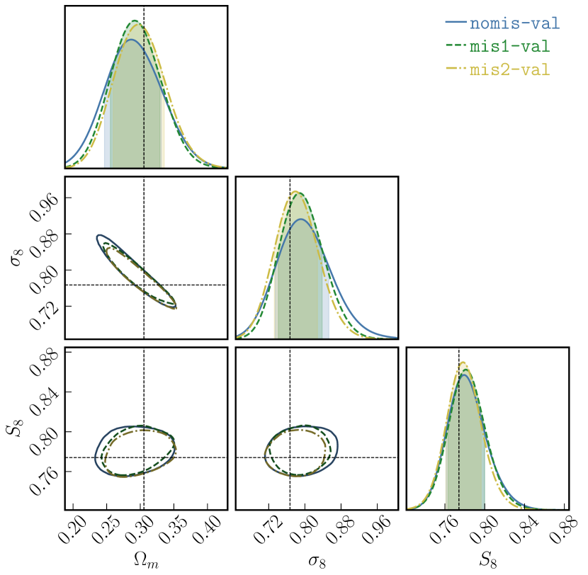
Figure 3: The 68% confidence regions for cosmological parameters of interest, obtained by running our fiducial pipeline on the validation mocks. The different colored regions represent results from different variations of the validation mock: no miscentering (blue); miscentered according to Equation 17 but with unknown parameters (green); and miscentered with a model different from Equation 17, again with unknown parameters (yellow). Dashed lines represent the input cosmology for the mocks.

The successful validation of our model and analysis choices offers an encouraging answer to the first research question we posed in Section 1. That is, our analysis enables the combination of cluster abundances, lensing, and clustering to simultaneously achieve tight cosmological constraints and self-calibrations of key systematics without informative priors or calibrations. Compared to previous cluster cosmology studies, our approach adds an additional model dimension of freedom with the anisotropic boosts, but at the same time incorporates a new constraint by including cluster clustering. This could partially explain why our model can successfully obtain tight cosmological constraints despite the added freedom from anisotropic boosts. However, it is still surprising to see that all of our systematics are correctly self-calibrated without priors or external calibrations, in particular for miscentering. Considering that we do not see significant degeneracies between miscentering parameters and cosmology in our posteriors, we postulate that the model behavior induced by miscentering is quite orthogonal to cosmological signatures. This would then imply that even a rough accounting for miscentering, as we do in this work with a simple, freely varied Rayleigh distribution, would successfully mitigate the impact of miscentering on cosmological constraints.

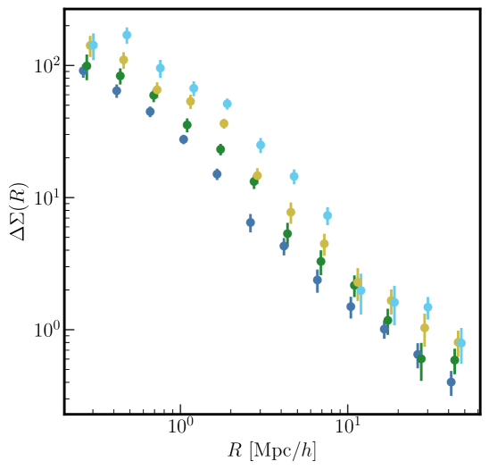
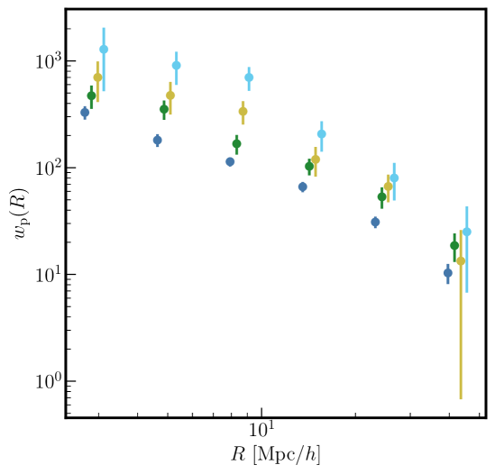
Figure 4: Left: Cluster abundance measurements from the SDSS RM catalog. Horizontal bars represent our number counts, and the shaded regions represent the 1-$\sigma$ uncertainties. The colors correspond to our richness bins. Center: Cluster lensing measurements and 1-$\sigma$ uncertainties for the four richness bins. Points are offset horizontally for visibility. Right: Same as the center panel but for cluster clustering measurements.

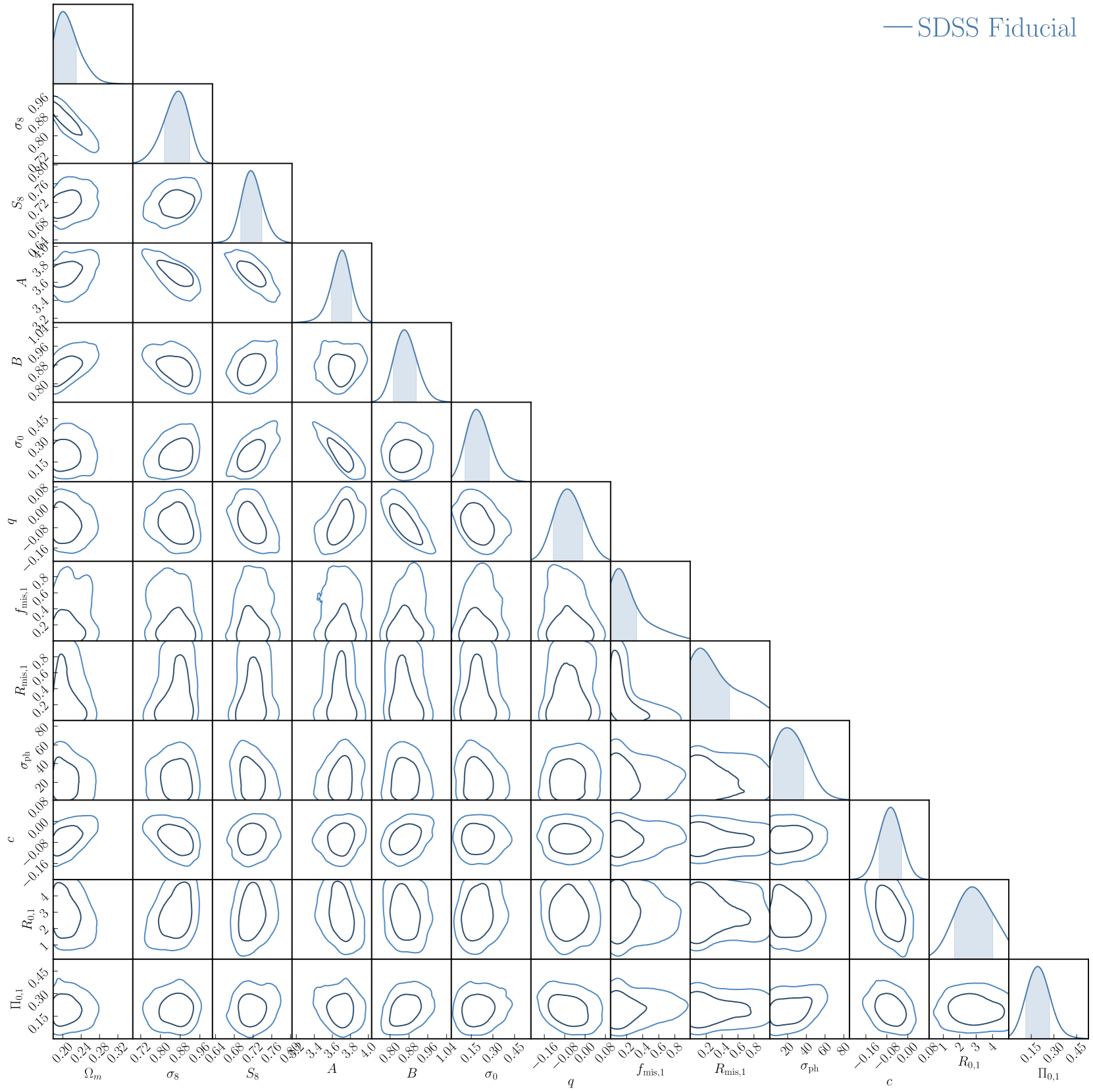
Figure 5: The 68% and 95% confidence regions from our fiducial analysis combining SDSS RM cluster abundances, lensing, and clustering. We show here three derived cosmological parameters of interest, four MOR parameters, three systematics parameters for miscentering and cluster photo-$z$ scatter, and three anisotropic boost parameters. For richness bin specific parameters, we only show here results for the first richness bin, and present the rest of the results in Appendix B.

4 Application to SDSS redMaPPer clusters

4.1 Data

With our model and analysis choices successfully validated, we now move to apply the framework on real data. We use version 6.3 of the SDSS redMaPPer (RM) cluster catalog (Rykoff et al., 2014; Rozo & Rykoff, 2014; Rozo et al., 2015a, b), based on the SDSS Data Release 8 (Aihara et al., 2011) photometry. This catalog covers 10,401 $\mathrm{deg}^{2}$, and we use a total of 8,379 clusters within the richness range $\lambda\in[20,200)$ and the redshift range $0.1\leq z\leq 0.33$. The redshift range chosen ensures that the RM catalog is very nearly volume-limited. As mentioned in Section 2.1, we choose a single representative redshift for this range, $z=0.25$, in calculating model predictions. For cluster lensing measurements, we follow the methodology of Mandelbaum et al. (2013) and Miyatake et al. (2016), using the shape catalog from Reyes et al. (2012). This shape catalog consists of shapes for 39 million galaxies measured via the re-Gaussianization technique (Hirata & Seljak, 2003), over a $\sim$9,000 $\mathrm{deg}^{2}$ overlap with the RM catalog. The shape measurement systematics in this catalog were extensively studied following the procedures defined in Mandelbaum et al. (2005), and the image simulations used to calibrate the shape measurements are described in Mandelbaum et al. (2012). We use the ZEBRA (Feldmann et al., 2006; Nakajima et al., 2012) photometric redshifts for these sources.

4.2 Measurements

Our analysis consists of three sectors of observables: cluster abundances, cluster lensing, and cluster clustering. In some cases we will respectively refer to these sectors as NC, DS, and WP from here on. To measure cluster abundances, we start with the number counts of clusters in the RM catalog corresponding to each of our richness bins, i.e, for $\lambda\in[20,30),~{}[30,40),~{}[40,55),~{}[55,200)$. The cluster counts, however, are impacted by the detection efficiency of the RM catalog; survey geometries such as masks and boundaries will prevent some clusters from being properly detected. We thus use the richness-dependent detection efficiencies from Murata et al. (2018), calculated on the exact same catalog as ours, to correct for the missed detections. Also, a background cosmology must be assumed for the following measurement calculations. Under a flat $\Lambda$CDM model the only relevant parameter is $\Omega_{\mathrm{m}}$, and we set it to 0.27 in making the measurements. In the subsequent likelihood analyses, we take this assumption into account by introducing a correction to our theoretical predictions, following More (2013).

For lensing, our estimator for $\Delta\Sigma(R)$ is given by

$$\widehat{\Delta\Sigma}(R)=\frac{\sum_{\mathrm{ls}}w_{\mathrm{ls}}e_{\mathrm{t,ls}}\Sigma_{\mathrm{crit,ls}}}{[1+\hat{m}(R)]\sum_{\mathrm{ls}}w_{\mathrm{ls}}},$$ (25)

where the subscripts $\mathrm{l}$ and $\mathrm{s}$ runs over all lenses and sources considered, $e_{\mathrm{t,ls}}$ is the tangential ellipticity for a given lens-source pair, $\Sigma_{\mathrm{crit,ls}}$ is the point estimate for the critical surface density corresponding to the lens-source pair given by

$$\Sigma_{\mathrm{crit,ls}}=\frac{c^{2}}{4\pi G(1+z_{\mathrm{l}})}\frac{\chi_{\mathrm{s}}}{\chi_{\mathrm{l}}\chi_{\mathrm{ls}}},$$ (26)

with the lens redshift $z_{\mathrm{l}}$, comoving distances to the lens and source $\chi_{\mathrm{l}}$ and $\chi_{\mathrm{s}}$, and the comoving distance between the lens and the source $\chi_{\mathrm{ls}}$. The lens-source pair weight $w_{\mathrm{ls}}$ is given by

$$w_{\mathrm{ls}}=w_{\mathrm{l}}w_{\mathrm{s}}\Sigma_{\mathrm{crit,ls}}^{-2}$$ (27)

with the lens and source weights $w_{\mathrm{l}}$ and $w_{\mathrm{s}}$. Note that in our case the lens weights are always unity; the source weights are given by the source catalog. The factor $[1+\hat{m}(R)]^{-1}$ corrects for an overall multiplicative shear bias as a function of $R$ (Miller et al., 2013).

We then apply three different corrections to the raw estimated $\Delta\Sigma(R)$. First, we calibrate the measurements for source photo-$z$ biases following Equation 21 of Nakajima et al. (2012). This calculation yields a lens redshift dependent bias factor for $\Delta\Sigma$, and we multiply this factor to our measurements. Next, we apply boost factor corrections to account for potential dilutions in the lensing signal from cluster members being mistaken as background sources. The boost factor $\mathcal{B}(R)$ is given by

$$\mathcal{B}(R)=\frac{N_{\mathrm{r}}}{N_{\mathrm{l}}}\frac{\sum_{\mathrm{ls}}w_{\mathrm{l}}w_{\mathrm{s}}}{\sum_{\mathrm{rs}}w_{\mathrm{r}}w_{\mathrm{s}}},$$ (28)

where the new subscript $\mathrm{r}$ refers to the random catalog for RM clusters, with the total number of randoms $N_{\mathrm{r}}$ and weights $w_{\mathrm{r}}$. The measured signal is then multiplied with $\mathcal{B}(R)$. Finally, we estimate the $\Delta\Sigma(R)$ signal around the randoms and subtract this random signal from our measurements. The random signal detects coherent tangential shear around random points, which should vanish under perfect conditions, and removing it helps account for residual errors in the shape measurements and calibrations.

For the final sector of cluster clustering, we use the Landy-Szalay estimator (Landy & Szalay, 1993) to first estimate $\xi_{\mathrm{cc}}$ as

$$\widehat{\xi}_{\rm cc}=\frac{\left<DD\right>-2\left<DR\right>+\left<RR\right>}{\left<RR\right>},$$ (29)

Where $DD$, $DR$, and $RR$ are the normalized number of cluster-cluster, cluster-random, and random-random pairs, respectively. For the randoms, we use the publicly available RM random catalog. The measured $\xi_{\mathrm{cc}}$ is then converted to $w_{\mathrm{p}}(R)$ using Equation 13, with $\pi_{\mathrm{max}}=100~{}\mathrm{Mpc}/h$.

For our likelihood analyses, we use a jackknife resampling of our data vector with 83 independent regions to estimate our covariances. As in Section 3, we assume a block-diagonal covariance matrix by treating the 9 sections of our data vector (abundances, 4 lensing profiles, and 4 autocorrelation functions) as independent from one another. We also apply the Hartlap correction (Hartlap et al., 2007) to perform a basic debiasing of our inverse covariance matrix used in the likelihood calculations. We show our measurements and their 1-$\sigma$ uncertainties in Figure 4. As the SDSS RM catalog and the associated observables we use have already been thoroughly studied and published, we do not consider a measurement level blinding for our analysis. Our blinding thus is limited to the analysis choice side, where we completely freeze the exact specifications of our fiducial analysis in Section 3.1 and apply it to both the validation in Section 3.2 and the real data analysis below.

4.3 Results

We show the results from our fiducial analysis on SDSS RM clusters in Figure 5. We consider this analysis blinded in the same way our validation was blinded, as we use the same frozen model from Section 3.1, which was developed without any use of the SDSS data, for our results. Given the recent issues pointed out in Lemos et al. (2022) that the multinest sampler may have trouble in obtaining the correct credible intervals for the sampled parameters, we tested both multinest and polychord samplers in sampling our posteriors. We find that while the two samplers yield very similar posterior centers, polychord yields wider credible intervals than multinest at the level of tens of per cents. We thus choose to use polychord for all of our real data results, which we consider as a conservative choice in line with the recommendations of Lemos et al. (2022).

Due to limits in the parameter space coverage of darkemu, in particular the lower limit of $\Omega_{\mathrm{m}}\gtrsim 0.18$, our posterior is truncated at around the 68% contour on the low-$\Omega_{\mathrm{m}}$ end. This prevents us from robustly quantifying our cosmological posteriors, but the $S_{8}$ constraints are the least affected by the truncation and we report $S_{8}=0.715_{-0.021}^{+0.024}$. We also find that our posterior favors significantly lower $\Omega_{\mathrm{m}}$ and consequently $S_{8}$ values than other CMB/LSS results. Figure 6 further clarifies this tendency; compared against Planck 2018 (Planck Collaboration et al., 2020) results, we find significantly lower constraints for both $\Omega_{\mathrm{m}}$ and $S_{8}$. The rest of the parameter space shown consists of 4 MOR parameters ($A$, $B$, $\sigma_{0}$, and $q$), 2 miscentering parameters ($f_{\mathrm{mis,1}}$ and $R_{\mathrm{mis,1}}$), the photo-$z$ scatter ($\sigma_{\mathrm{ph}}$), and 3 anisotropic boost parameters ($c$, $R_{0,1}$, $\Pi_{0,1}$). For richness bin specific parameters (miscentering and anisotropic boost) we only show results for the first bin, but note that the results are consistent across all richness bins. The full constraints for these bin-specific parameters are shown in Figures 13 and 14. We find a best fit $\chi^{2}/\mathrm{dof}$ of $42.3/49$.

Let us take a closer look at the non-cosmology posteriors. First, we find that our systematics parameters are successfully self-calibrated. We find anisotropic boost amplitudes ranging between 15–20%, which matches our findings from simulations as well as the observational constraints from To et al. (2021). We also find miscentering fractions $\sim$ 15% and miscentering scales around 0.2–0.3 Mpc$/h$, consistent with X-ray studies on the same cluster sample (e.g. Miyatake et al., 2016; Zhang et al., 2019). The degree of cluster photo-$z$ scatter is determined to be $\sim$ 20 Mpc$/h$, which again is consistent with the performance of the RM photo-$z$ estimation. Turning our attention to the degeneracies between the cosmological parameters and the rest of the parameter space, we find that beyond the MOR parameters, which are inherently correlated with cosmology, the only model parameter that shows a meaningful degeneracy with $\Omega_{\mathrm{m}}$ and $S_{8}$ is $c$. If we imagine extrapolating the degeneracy between $c$ and cosmology, $c\sim 0$ would result in cosmological constraints much closer to existing results. As presented in Equation 16, $c$ represents the (generally negative) slope of the logarithmic decay in the effective bias $\Pi(R)$. A stronger (more negative) $c$ has the effect of suppressing the cluster clustering signal, while slightly enhancing the large scale regime of the cluster lensing signal. We investigate this degeneracy further in Section 5.

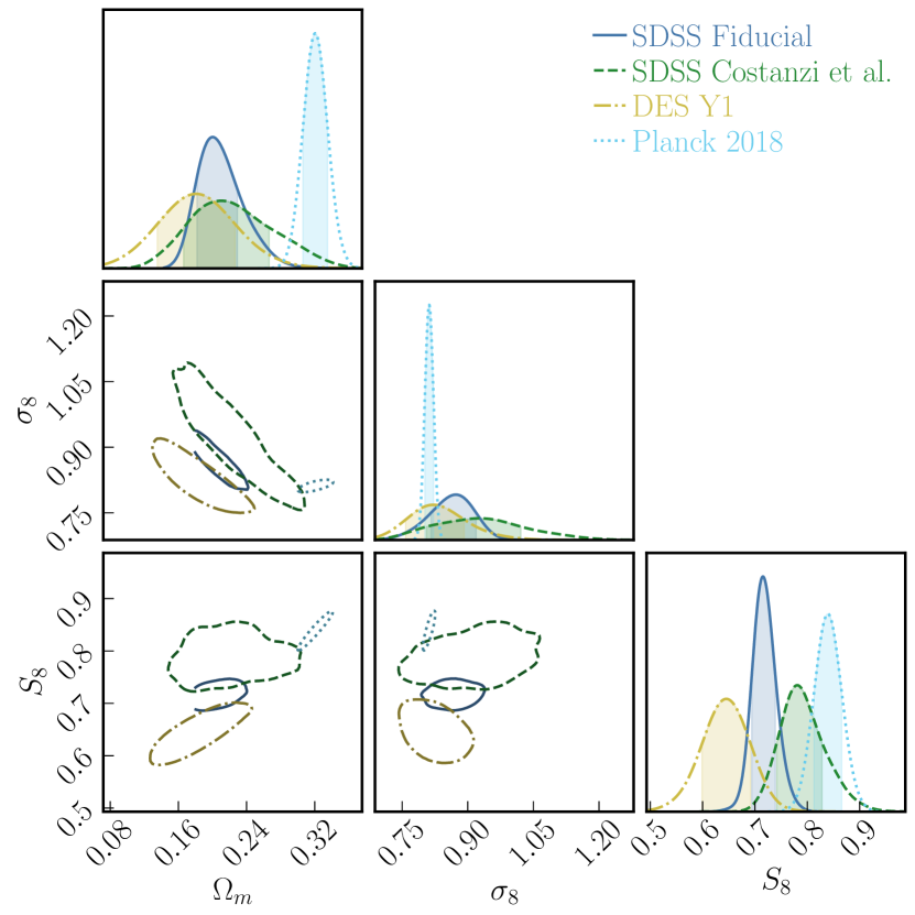
Figure 6: Comparison of 68% confidence regions for cosmological parameters of interest from our fiducial results (blue) with relevant previous results: Costanzi et al. (2019) in green, DES Collaboration et al. (2020) in yellow, and Planck Collaboration et al. (2020) in light blue.

In addition, Figure 6 shows an interesting consistency between previous cluster cosmology results and ours. Both the Costanzi et al. (2019) and the post-unblinding DES Collaboration et al. (2020) results center around lower $\Omega_{\mathrm{m}}$, and to some degree $S_{8}$, values, that are consistent with our findings. The differing approaches taken by these three cluster cosmology results make this consistency particularly intriguing. The analysis of Costanzi et al. (2019) uses virtually the same abundance and lensing data as ours, coupled with a more complex mass-observable relation and systematics models calibrated from simulations. They do not, however, explicitly model the impact of anisotropic boosts on the lensing signal. DES Collaboration et al. (2020), on the other hand, uses a completely independent data set, inherits the modeling of Costanzi et al. (2019), and calibrates the impact of anisotropic boosts on the weak lensing mass calibrations in their post-unblinding results using simulations. The two existing cosmology studies also vary the sum of neutrino masses in their analyses, while we fix it in our analysis. Considering these different combinations of models and data sets used, the consistently low $\Omega_{\mathrm{m}}$ found by all three results could suggest an unknown systematic effect or physics in clusters that cannot be localized to a particular data set or analysis method.

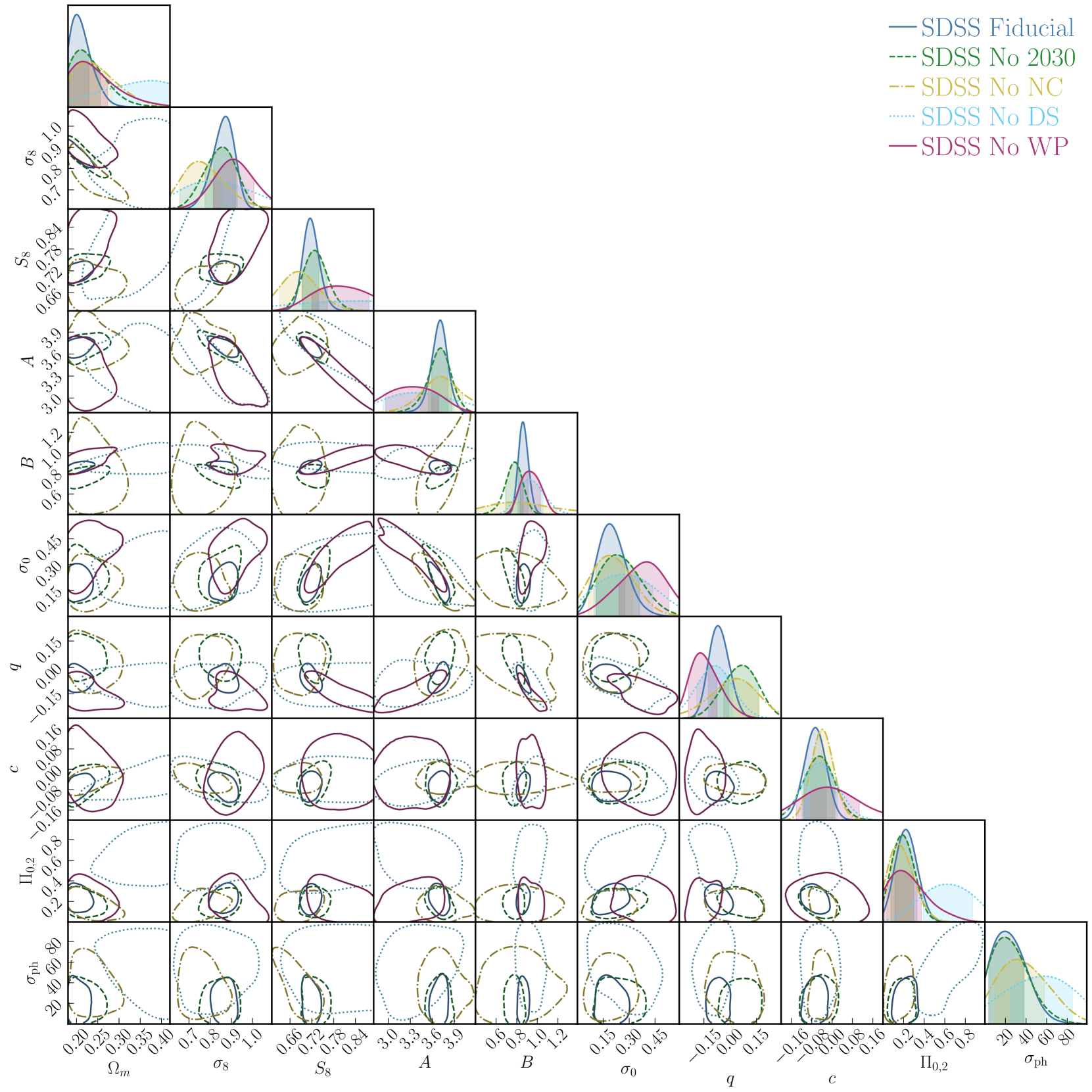
Figure 7: Comparison of 68% confidence regions for model parameters when varying our analysis choices. Here we show the results from excluding the lowest richness bin (“No 2030”), the abundance information (“No NC”), the lensing information (“No DS”), and the clustering information (“No WP”). We omit several parameters we show in Figure 5, as they do not show meaningful impacts on the cosmology results. Note that we have “zoomed in” toward the fiducial posterior center for readability.

5 Post-unblinding analyses

5.1 Varying analysis choices

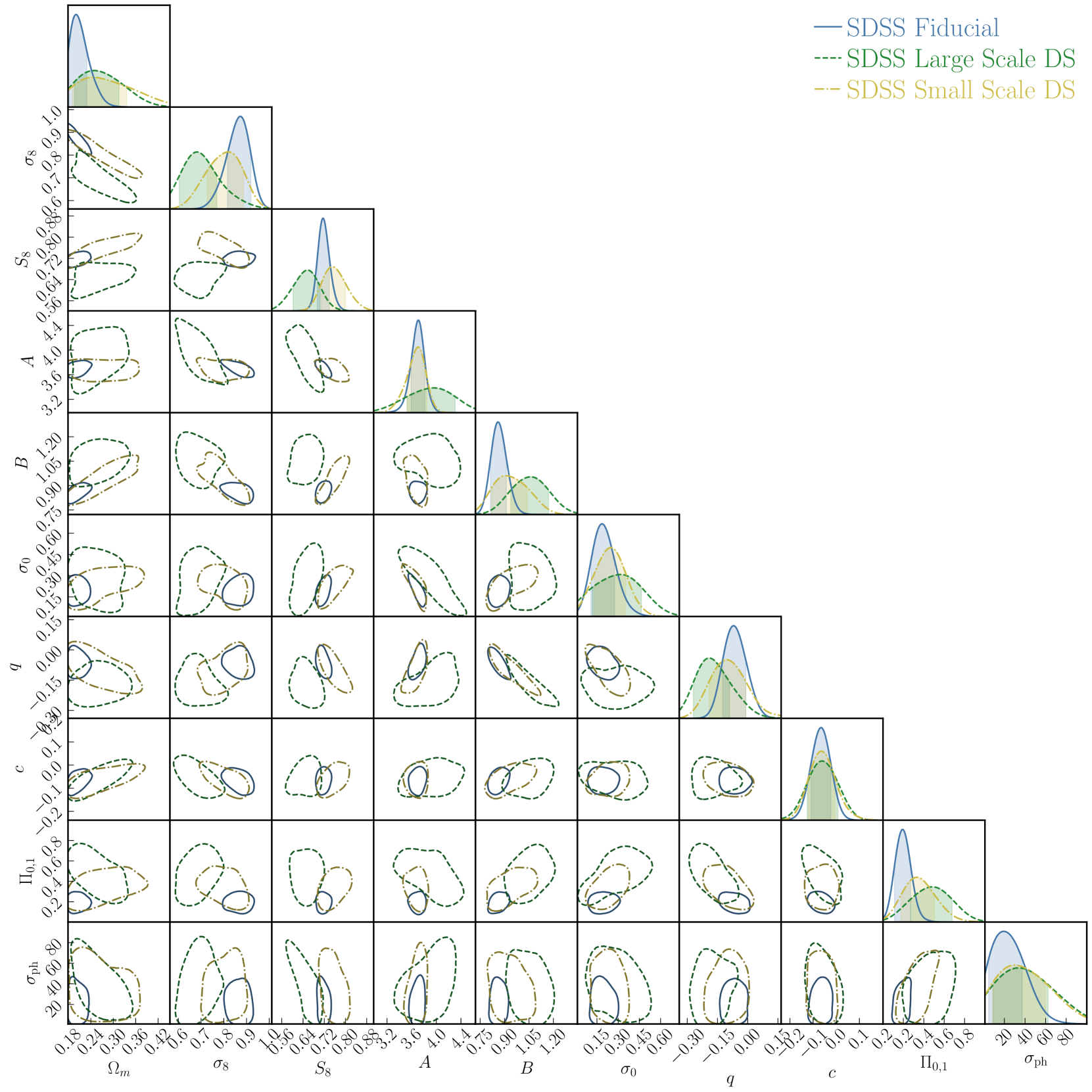
Figure 8: Similar to Figure 7, but now varying the range of scales used for the cluster lensing signal. Here we show the 68% confidence regions from our fiducial results (blue), as well as from restricting the range of scales for $\Delta\Sigma(R)$ to $R\geq 8~{}\mathrm{Mpc}/h$ (green) and $R<8~{}\mathrm{Mpc}/h$ (yellow).

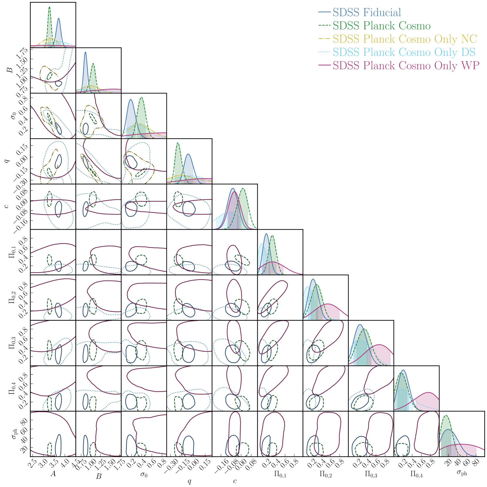
Figure 9: Comparison of 68% confidence regions for MOR and anisotropic boost parameters when fixing the cosmology to the Planck 2018 best fit and using individual sections of the data vector. We show fixed cosmology results using abundance information only (“Only NC”), lensing information only (“Only DS”), and clustering information only (“Only WP”). We also show the results from our fiducial analysis (blue; note that this does not assume a Planck cosmology), as well as fixed cosmology results using the full data vector (green), for reference. Note that we have “zoomed in” toward the fiducial posterior center for readability, as we did in Figure 7.

To better understand the driver behind our low-$\Omega_{\mathrm{m}}$ results, we perform a number of post-unblinding analyses. We begin with the argument in DES Collaboration et al. (2020) that their measured lensing signal, in particular for the lowest richness bin, is lower than expected. Following this insight, we test in Figure 7 whether dropping the lowest richness bin ($20\leq\lambda<30$), or any one sector of our data vector (abundances, lensing, and clustering), impacts our conclusions. The results we find, however, are inconclusive with respect to the DES Y1 argument. While dropping the lowest richness bin leads to wider confidence regions, the posterior peaks for the cosmological parameters stay the same. Note that any potential broadening of uncertainties toward even lower $\Omega_{\mathrm{m}}$ would be truncated by our lower limit of $\Omega_{\mathrm{m}}\geq 0.18$. Dropping the entire lensing data does pull our results to higher $\Omega_{\mathrm{m}}$, but we also suffer a heavy loss in constraining power as the lensing information is our main cluster mass calibrator. Another notable aspect is that when we exclude WP, we find that our $S_{8}$ constraints shift higher. As a result, our “No WP” results become consistent with Costanzi et al. (2019) in the $\Omega_{\mathrm{m}}-\sigma_{8}$ plane, and our marginalized $S_{8}$ constraints become consistent with other CMB/LSS based results. However, the low-$\Omega_{\mathrm{m}}$ issue is still persistent, and the posteriors are truncated, so we remain cautious in further interpreting this shift. We finally note that in plotting the posteriors we have “zoomed in” toward the posterior center of our fiducial result at the cost of cutting off some of the wider contours, in order to make the tighter confidence regions readable.

This exercise offers a number of insights on our fiducial results as well. First, we find that excluding any sector of the data vector leads to a significant loss of constraining power. While this is somewhat expected for NC or DS, it is interesting to see that excluding WP brings noticeable changes. This implies that cluster autocorrelation functions may be playing an important role in breaking the degeneracy among $\sigma_{8}$, cluster bias, and anisotropic boosts, all of which similarly affect the large-scale lensing and clustering amplitudes. Also, considering that results from simulations and observations, as well as results comparing galaxy autocorrelations against cluster-galaxy cross-correlations (Sunayama, 2022) suggesting anisotropic boost strengths around 20%, the “No DS” amplitudes of 60–70% are not likely to be genuine. In addition, examining the $\Omega_{\mathrm{m}}-c$ and $\sigma_{8}-c$ planes clarify the driver behind the degeneracies among these parameters we found in our fiducial result. While every other result in Figure 7 shows similar degeneracies between $\Omega_{\mathrm{m}}/\sigma_{8}$ and $c$, the “No WP” result clearly departs from this tendency. This suggests that the clustering sector of our data, and more specifically the significant impact of $c$ on the predicted clustering amplitude, is correlating $c$ with the cosmological parameters of interest. As the “No WP” result also favors low values of $\Omega_{\mathrm{m}}$, it is difficult to argue that $c$, or its degeneracy with cosmological parameters, is responsible for our low $\Omega_{\mathrm{m}}$ results.

Noting that excluding lensing was the only variation we found to result in shifted cosmological constraints, we further test the lensing sector of our data vector in Figure 8, where we limit the range of scales used in our cluster lensing signal to small scales only ($R<8~{}\mathrm{Mpc}/h$) and large scales only ($R\geq 8~{}\mathrm{Mpc}/h$). Both variations result in posteriors favoring higher $\Omega_{\mathrm{m}}$, but similar to the “No DS” case these results accompany changes in the MOR and anisotropic boost parameter constraints. When only the small scale lensing data is used, parameter constraints show a broadening of the constraints along the degeneracy directions, and the $S_{8}$ constraints shift higher. As for the large scale lensing only case, the changes have different characteristics, and involve larger departures from the fiducial result in MOR and anisotropic boost parameters as well as even lower values of $S_{8}$. Limiting ourselves to the cosmological parameters, we find that both the “Small Scale DS” and “Large Scale DS” results are consistent with the “No DS” results, with the former slightly more so than the latter. Note that the small scale lensing signal probes cluster masses with a higher signal-to-noise, as well as a weaker contribution from anisotropic boosts, compared to its large scale counterpart. This explains the wider confidence regions seen from the “Large Scale DS” results: without the small scale lensing information our model finds it more difficult to constrain parameters related to mass calibration.

We end this section by cautioning the reader that all of the results presented in Figures 7 and 8 are correlated with one another, as any given pair of the results shown shares in common at least one sector of the data vector. This, in addition to the fact that our cosmology posteriors are necessarily truncated at the parameter limits of the Dark Emulator, prohibits straightforward quantifications of differences, or tensions, between these results. We thus leave the task of formally estimating the statistical significance of these tensions as future work.

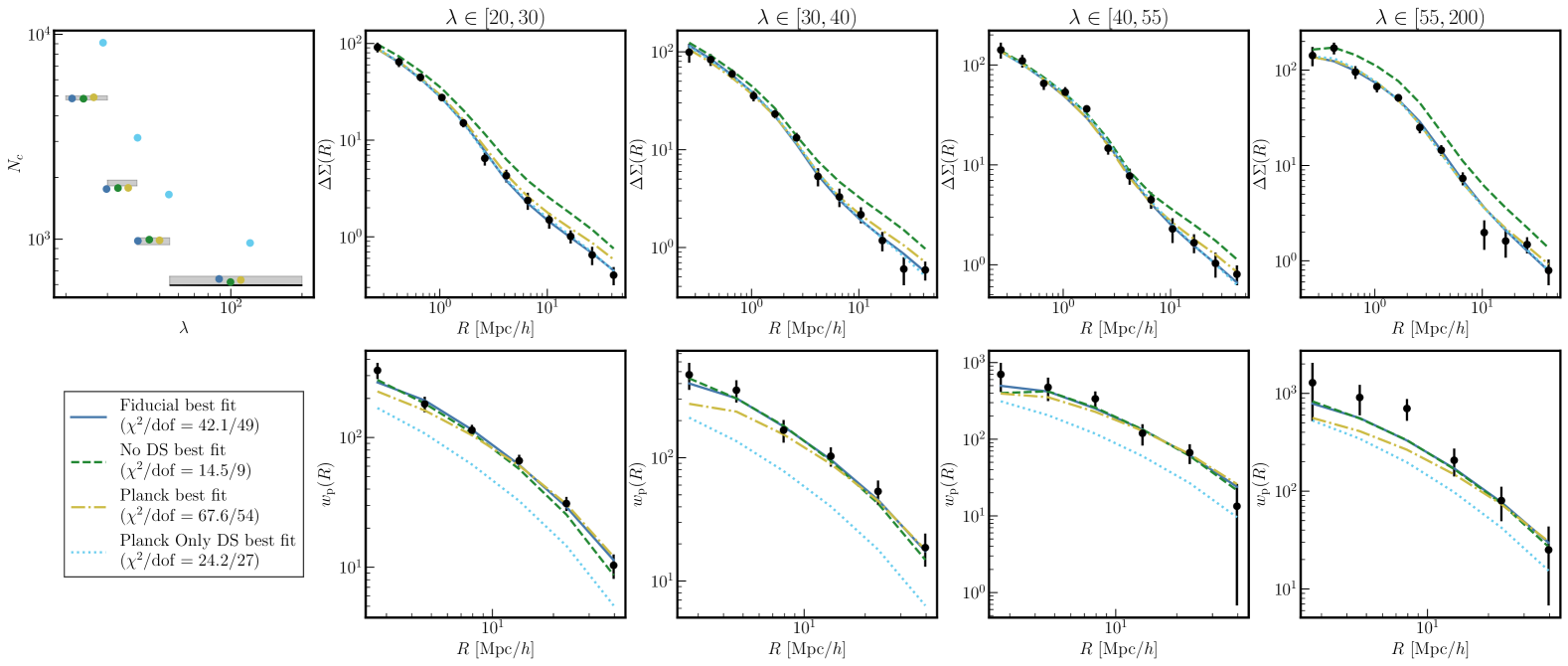
Figure 10: Comparison of our measurements with the best-fit predictions from the fiducial analysis and selected post-unblinding tests. We show cluster abundance comparisons in the top left panel, and the cluster lensing (top row) and cluster clustering (bottom row) comparisons in the next four columns, with each column corresponding to a richness bin we analyze. The bests fits shown are from the fiducial analysis (blue), the “No DS” analysis (green), full data analysis under Planck cosmology (yellow), and the “Only DS” analysis under Planck cosmology (light blue).

5.2 Fixing cosmological parameters

The results in Section 5.1 do not offer a straightforward interpretation. Removing lensing from the analyzed data shifts cosmological constraints closer to existing results, but the surprisingly high strength of anisotropic boosts predicted makes it difficult to take at face value. Using subsets of the lensing data does not produce a clear picture either; using only large scale lensing yields even lower values of $S_{8}$, and it is difficult to tell whether the small scale lensing only results are exhibiting genuine shifts in cosmological constraints or a mere broadening of the contours. At the same time, no other exclusion of data vector sectors or richness bins seem to have a significant effect on the low values of our marginalized $\Omega_{\mathrm{m}}$ constraints. To decouple the different elements at play, we now fix our cosmology to the Planck 2018 best fit and consider only the non-cosmological parameter space.

As fixing the cosmology significantly shrinks the parameter space and the degeneracies therein, we can take a step further from Section 5.1 and derive constraints using individual sectors of our data vector, in addition to using the full data set combination. Figure 9 shows the results from this exercise, and this further illuminates how each sector drives the MOR and anisotropic boost constraints. Note that we are again “zooming in” for readability, as we did above in Figure 7. Starting with the full data analysis under fixed cosmology, we first note that the results favor an MOR that is clearly different from the fiducial results. More specifically, we see the new preferred MOR has a lower normalization ($A$), a steeper slope ($B$), a larger intrinsic scatter ($\sigma_{0}$), and a stronger mass-dependent scatter ($q$). We also find shifts in the anisotropic boost constraints, with the fixed cosmology results preferring (i) $c\sim 0$ and (ii) slightly larger, and richness dependent, boost amplitudes. The richness dependence of the $\Pi_{0,i}$ parameters was not apparent in any of our earlier results.

Turning our attention now to single sector constraints, we immediate notice that the “Only NC” result shows a clear bimodality in its MOR constraints. Interestingly, the two modes of this posterior closely follow the respective preferred MORs of the fiducial and the fixed cosmology full data analyses. It is surprising to see that the fiducial MOR is still one of two preferred modes, as this was derived under a very different cosmology from the one assume here. The “Only DS” results also show MOR constraints compatible with both of these modes, and the “Only WP” MOR constraints are too wide to interpret with significance. As for the anisotropic boost parameters, we note that the “Only WP” results favor boost strengths that are significantly higher and even more richness dependent than the full analysis. The higher strengths are in line with the “No DS” results from Figure 7, and may be related to fact that the photo-$z$ scatter, largely unconstrained and thus generally higher than the full analysis best fit, ends up suppressing the predicted WP signals more. The richness dependence, on the other hand, may suggest that the bias-mass relation dictated by the Planck cosmology, combined with our model, is not compatible with the measured amplitudes of the cluster autocorrelation functions. The “Only DS” results, on the other hand, prefer weaker boost strengths, also weakly richness dependent, but are generally consistent with the full analysis results.

Let us consolidate our findings in the data space with Figure 10. Here we compare our measurements with the best fit predictions from our fiducial analysis and a number of relevant post-unblinding tests. We focus in particular on the DS sector, as the “No DS” result was the only result we saw with any shift in the $\Omega_{\mathrm{m}}$ posterior center. Beginning with the fiducial best fit, we find good agreement across all sectors between measurements and predictions. When lensing is removed from this analysis, the preferred cosmology becomes consistent with Planck and the MOR also shifts. The resulting predictions, shown in green, fit the measurements included in the analysis (NC and WP) well but overpredicts lensing, in particular on large scales. Note that since the “No DS” fits do not include miscentering parameters, we use their best fit values from the fiducial analysis to generate lensing predictions. Next, with the cosmology fixed to the Planck 2018 values, the resulting best fit again slightly overpredicts lensing on large scales, and this time the clustering signal is underpredicted. This “compromise” between the lensing and clustering sectors, compared to the fiducial “No DS” prediction, is likely driven by the fact that lensing dominates in the signal-to-noise over clustering. In addition, the degradation in the goodness-of-fit, from $\chi^{2}/\mathrm{dof}$ of $42.1/49$ to $67.6/54$, illustrates potential internal tensions between the different data sectors when assuming a Planck cosmology.

Finally, when we assume the Planck cosmology and fit only the lensing data, we note significant overpredictions in the cluster abundances and underpredictions in the clustering. This presents the clearest message among all of the post-unblinding tests that we have performed: under a Planck cosmology, our lensing data vector underpredicts cluster masses, leading to overpredicted abundances and underpredicted clustering amplitudes. Given the demonstrated completeness and purity of SDSS RM clusters, as well as the consistency of the mispredictions between the abundance and clustering sectors, the alternative interpretation — abundance measurements suppressed by a factor of two and clustering measurements inflated by a factor of two — is unlikely. The possibility of suppressed cluster lensing signals in our data is particular notable, as this is in line with findings from the DES Y1 cluster cosmology analysis. Considered together, we arrive at a stronger case for a significant missing element in our current understanding of cluster lensing.

6 Summary and Discussion

In this paper, we discussed the development and validation of a novel cluster cosmology analysis designed to be robust against the anisotropic boosts impacting the cluster lensing and cluster clustering observables, and the application of this analysis on the SDSS RM catalog to obtain cosmological constraints. Our work and findings can be summarized as follows.

• We accounted for the anisotropic boosts in the lensing and clustering signals around clusters with an empirical model taking the form of a scale-dependent effective bias. Upon validation with a blind cosmology challenge on mocks, this model was able to recover the expected degrees of anisotropic boosts on the lensing and clustering signals.

• We in addition find from our validation that by jointly analyzing cluster abundances, cluster lensing, and cluster clustering, especially across a wide range of scales using fully non-linear predictions from darkemu, we are able to obtain tight and unbiased constraints on the cosmological parameters of interest — $\Omega_{\mathrm{m}}$ and $\sigma_{8}$ — even with flat uninformative priors on all model parameters.

• After applying the pipeline to the SDSS RM catalog, we find cosmological constraints that strongly favor low $\Omega_{\mathrm{m}}$ and to a lesser degree $S_{8}$ values. We note that these results are interestingly consistent with recent attempts at cosmological constraints using clusters, but in strong tension with other CMB/LSS results.

• From a series of post-unblinding analyses, we find hints for internal tensions among the different sectors of our data set. Our most notable finding from these tests is that the cluster lensing signal we measure significantly underpredicts cluster masses when assuming a Planck cosmology. We are actively investigating the nature and origin of these findings.

The fact that our fiducial pipeline performed well on a blind challenge on mocks, but obtained somewhat suspicious (albeit with confirmation bias) cosmology results on real data, allows for informed guesses on the driver behind our cosmological constraints. Specifically, we may postulate that this driver is a subset of the differences between the mocks and the real data. Regarding the cluster lensing signal, the most likely driver behind our cosmology results, we note the difference in the way lensing is measured. In the mocks, we have the true underlying matter distribution, which we can readily project along the line-of-sight to calculate the lensing observable $\Delta\Sigma(R)$. In real data, however, we infer this quantity through the ellipticities of background galaxies, and effects that perturb the connection between ellipticities and matter densities, e.g., unmodeled intrinsic alignments, can complicate our findings. Such effects would cross boundaries of data sets and modeling approaches, and it would be very significant for cluster cosmology if we could point to a single cause that can explain the consistent disagreement between multiple cluster cosmology results and existing CMB/LSS cosmology constraints. The use of shape measurements from the Hyper Suprime-Cam SSP (HSC) survey (Li et al., 2021) may become particularly useful in investigating these effects. The HSC data overlaps with the SDSS RM footprint, but has significantly deeper photometry and better image quality than the SDSS source catalog, enabling source galaxy selections more robust to effects such as intrinsic alignments or source-cluster member confusion.

A deeper look into the characteristics of our model and data is also warranted. For instance, in modeling the impact of the anisotropic boosts we assume that the boost in clustering is the square of the boost in lensing, and carry it on all scales down to 2 Mpc$/h$. While this assumption has been successfully validated on mocks, we also know that tracer biases can deviate from this linear ansatz on small scales. It may be interesting to consider more flexibility on small scales for the anisotropic boost models, or to craft an entirely new approach based on an explicit model for the anisotropic LSS surrounding optical clusters. In addition, the flat uninformative priors we employ throughout our analysis may give rise to undetected parameter volume effects. Again, while we have not seen this in our validation, further checks on the real data results may bring surprises. We plan to explore all of the above possibilities in greater depth with follow-up studies in the near future, and we remain optimistic that these efforts will culminate in a robust analysis of clusters for precision cosmology.

Data Availability

The SDSS DR8 redMaPPer cluster and cluster member catalogs are publicly available at http://risa.stanford.edu/redmapper. The SDSS shape catalog used in this work is not publicly available; please contact Rachel Mandelbaum for inquiries on obtaining access.

Appendix A Full constraints from the Blind Validation

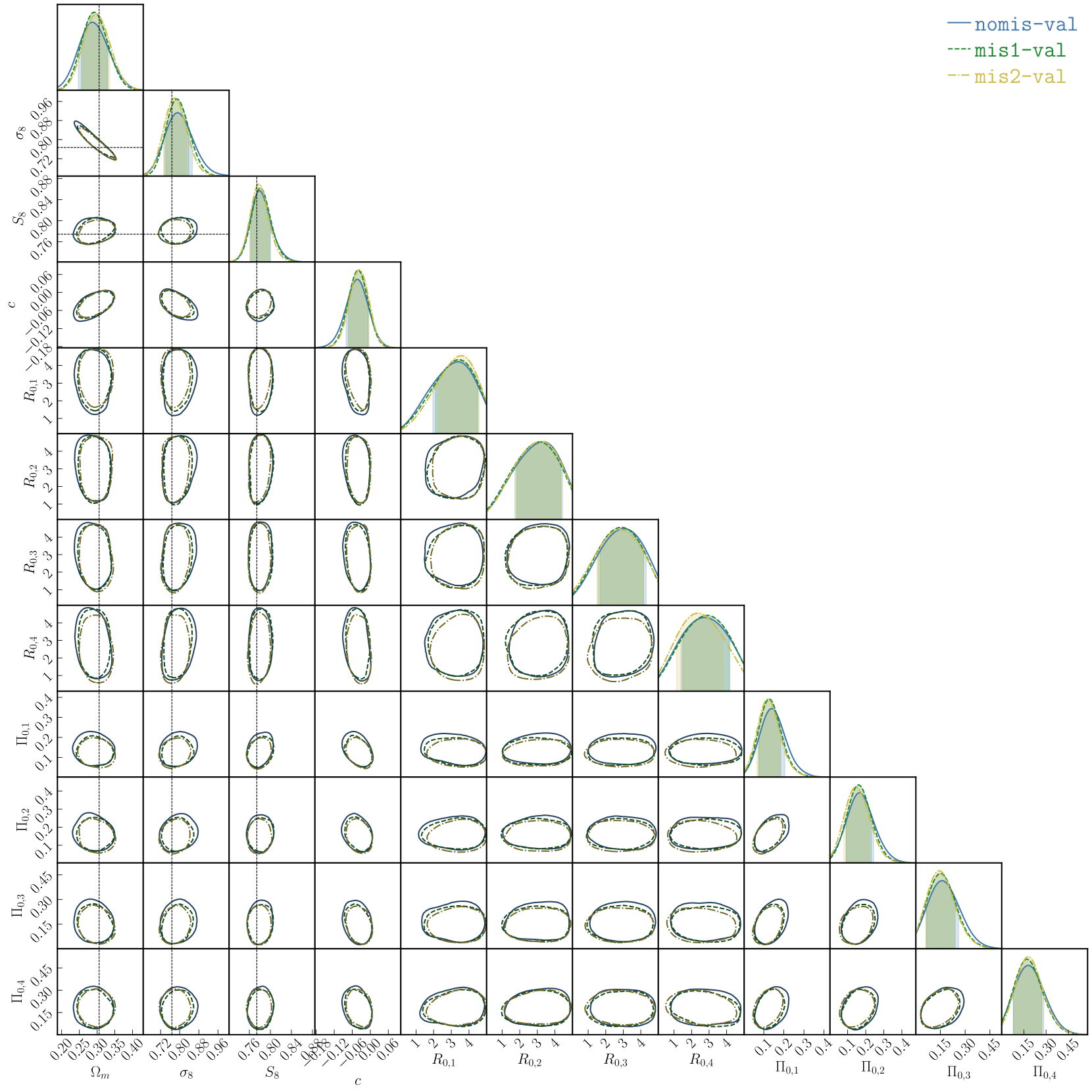
Figure 11: The 68% confidence regions for the full set of anisotropic boost parameters, along with the cosmological parameters of interest, from our validation analyses. We show results from all three variants of our validation test: nomis-val, mis1-val, and mis2-val.

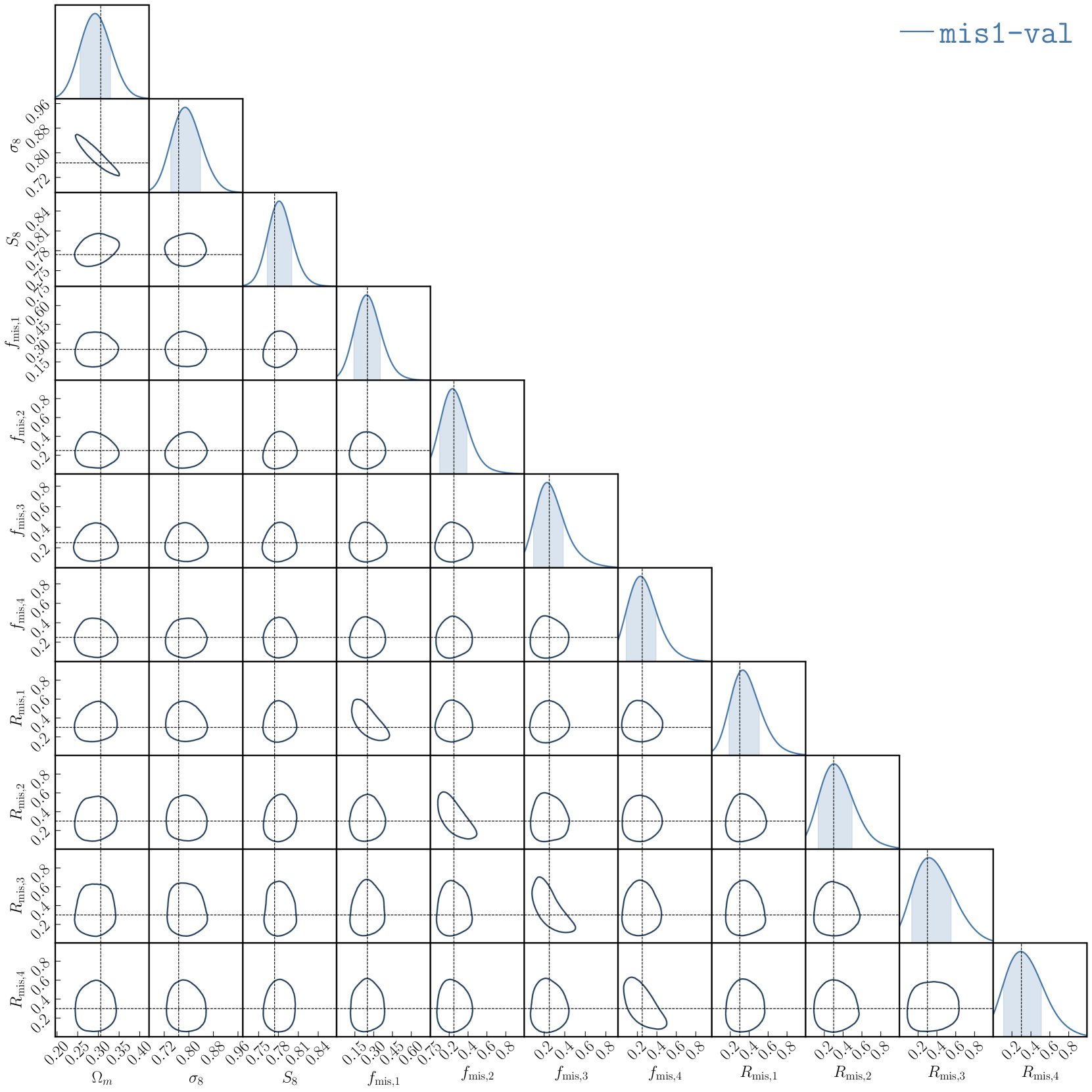
Figure 12: The 68% confidence regions for the full set of miscentering parameters, along with the cosmological parameters of interest, from our validation analysis. We only show the mis1-val results here, where the input and analysis miscentering models match.

We show here the full constraints from our validation analysis. Figures 11 and 12 respectively show the anisotropic boost and miscentering constraints we obtain, along with the cosmological parameters of interest. Note that for the latter we have the true input parameter values available, and we limit the constraints shown to the mis1-val case, where the input and analysis miscentering models match.

Appendix B Full constraints from the Fiducial SDSS RM Analysis

We show here the full constraints from our fiducial analysis for the bin-specific parameters. Figures 13 and 14 respectively show these results for the anisotropic boost and miscentering parameters, along with the cosmological parameters of interest. We note that the anisotropic boost and miscentering constraints show consistent behavior across all richness bins, despite being freely varied for each of these bins.

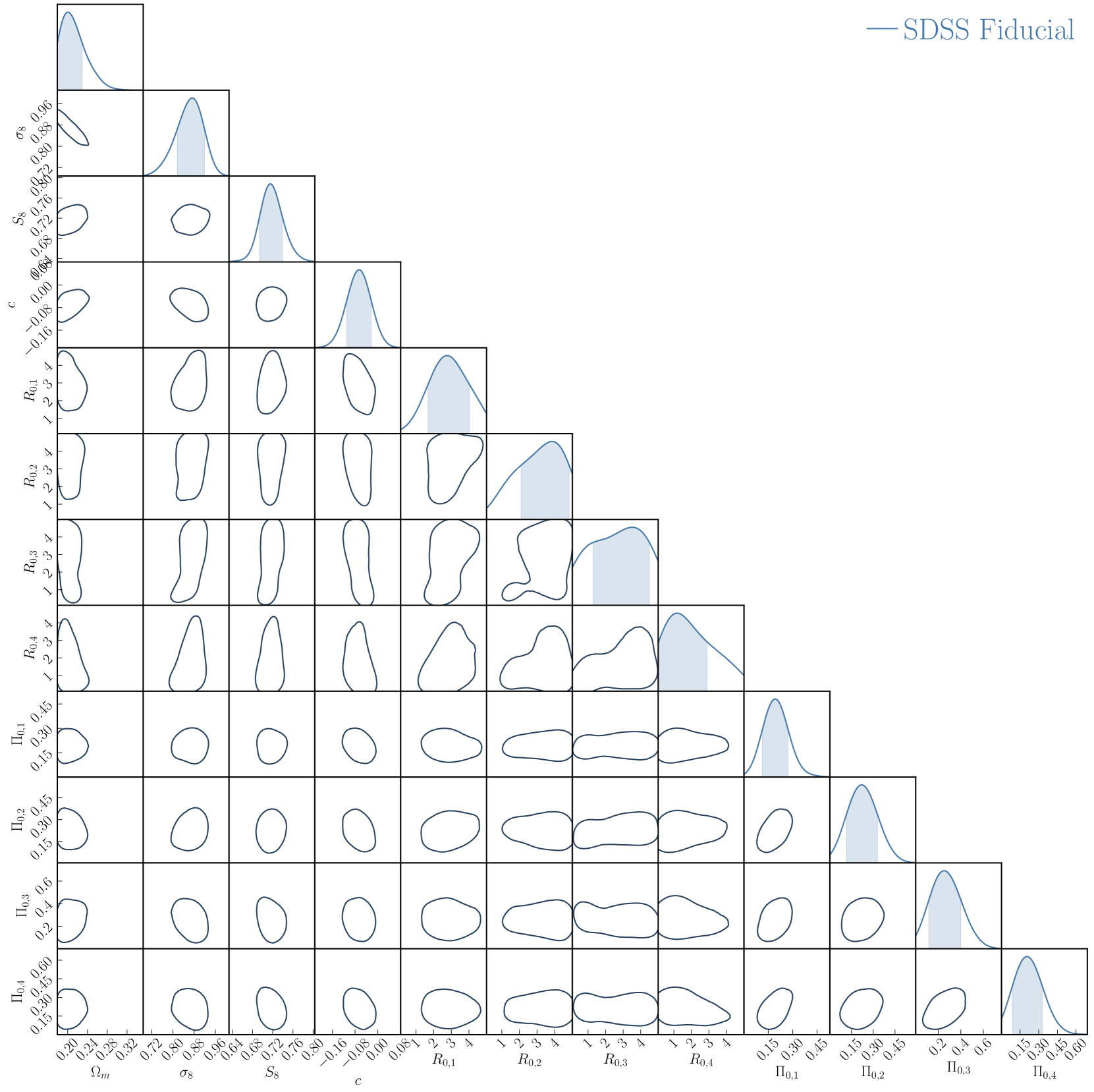
Figure 13: The 68% confidence regions for the full set of anisotropic boost parameters, along with the cosmological parameters of interest, from our fiducial analysis.

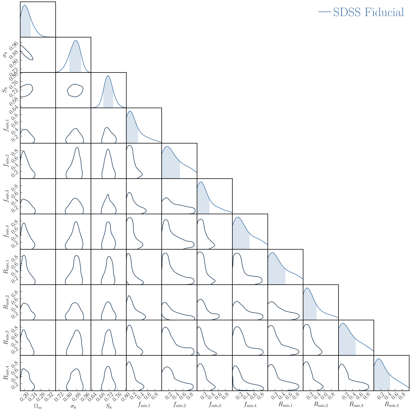
Figure 14: The 68% confidence regions for the full set of miscentering parameters, along with the cosmological parameters of interest, from our fiducial analysis.

References

- Aihara et al. (2011) Aihara H., et al., 2011, ApJS, 193, 29
- Allen et al. (2011) Allen S. W., Evrard A. E., Mantz A. B., 2011, ARA&A, 49, 409
- Bardeen et al. (1986) Bardeen J. M., Bond J. R., Kaiser N., Szalay A. S., 1986, ApJ, 304, 15
- Costanzi et al. (2019) Costanzi M., et al., 2019, MNRAS, 488, 4779
- DES Collaboration et al. (2020) DES Collaboration et al., 2020, Phys. Rev. D, 102, 023509
- Dawson et al. (2013) Dawson K. S., et al., 2013, AJ, 145, 10
- Dodelson et al. (2016) Dodelson S., Heitmann K., Hirata C., Honscheid K., Roodman A., Seljak U., Slosar A., Trodden M., 2016, arXiv e-prints, p. arXiv:1604.07626
- Feldmann et al. (2006) Feldmann R., et al., 2006, MNRAS, 372, 565
- Feroz & Hobson (2008) Feroz F., Hobson M. P., 2008, MNRAS, 384, 449
- Feroz et al. (2009) Feroz F., Hobson M. P., Bridges M., 2009, MNRAS, 398, 1601
- Feroz et al. (2019) Feroz F., Hobson M. P., Cameron E., Pettitt A. N., 2019, The Open Journal of Astrophysics, 2, 10
- Haiman et al. (2001) Haiman Z., Mohr J. J., Holder G. P., 2001, ApJ, 553, 545
- Handley et al. (2015a) Handley W. J., Hobson M. P., Lasenby A. N., 2015a, MNRAS, 450, L61
- Handley et al. (2015b) Handley W. J., Hobson M. P., Lasenby A. N., 2015b, MNRAS, 453, 4384
- Hartlap et al. (2007) Hartlap J., Simon P., Schneider P., 2007, A&A, 464, 399
- Hikage et al. (2013) Hikage C., Mandelbaum R., Takada M., Spergel D. N., 2013, MNRAS, 435, 2345
- Hinton (2016) Hinton S. R., 2016, The Journal of Open Source Software, 1, 00045
- Hirata & Seljak (2003) Hirata C., Seljak U., 2003, MNRAS, 343, 459
- Huterer et al. (2015) Huterer D., et al., 2015, Astroparticle Physics, 63, 23
- Johnston et al. (2007) Johnston D. E., et al., 2007, arXiv e-prints, p. arXiv:0709.1159
- Kaiser (1992) Kaiser N., 1992, ApJ, 388, 272
- Kravtsov & Borgani (2012) Kravtsov A. V., Borgani S., 2012, ARA&A, 50, 353
- Landy & Szalay (1993) Landy S. D., Szalay A. S., 1993, ApJ, 412, 64
- Lemos et al. (2022) Lemos P., et al., 2022, arXiv e-prints, p. arXiv:2202.08233
- Li et al. (2021) Li X., et al., 2021, arXiv e-prints, p. arXiv:2107.00136
- Lima & Hu (2005) Lima M., Hu W., 2005, Phys. Rev. D, 72, 043006
- Limber (1954) Limber D. N., 1954, ApJ, 119, 655
- Mandelbaum et al. (2005) Mandelbaum R., et al., 2005, MNRAS, 361, 1287
- Mandelbaum et al. (2012) Mandelbaum R., Hirata C. M., Leauthaud A., Massey R. J., Rhodes J., 2012, MNRAS, 420, 1518
- Mandelbaum et al. (2013) Mandelbaum R., Slosar A., Baldauf T., Seljak U., Hirata C. M., Nakajima R., Reyes R., Smith R. E., 2013, MNRAS, 432, 1544
- Mantz et al. (2015) Mantz A. B., et al., 2015, MNRAS, 446, 2205
- McClintock et al. (2019) McClintock T., et al., 2019, MNRAS, 482, 1352
- Miller et al. (2013) Miller L., et al., 2013, MNRAS, 429, 2858
- Miyatake et al. (2016) Miyatake H., More S., Takada M., Spergel D. N., Mandelbaum R., Rykoff E. S., Rozo E., 2016, Phys. Rev. Lett., 116, 041301
- Miyatake et al. (2021) Miyatake H., et al., 2021, arXiv e-prints, p. arXiv:2111.02419
- More (2013) More S., 2013, ApJ, 777, L26
- Murata et al. (2018) Murata R., Nishimichi T., Takada M., Miyatake H., Shirasaki M., More S., Takahashi R., Osato K., 2018, ApJ, 854, 120
- Murata et al. (2019) Murata R., et al., 2019, PASJ, 71, 107
- Nakajima et al. (2012) Nakajima R., Mandelbaum R., Seljak U., Cohn J. D., Reyes R., Cool R., 2012, MNRAS, 420, 3240
- Navarro et al. (1997) Navarro J. F., Frenk C. S., White S. D. M., 1997, ApJ, 490, 493
- Nishimichi et al. (2019) Nishimichi T., et al., 2019, ApJ, 884, 29
- Oguri (2014) Oguri M., 2014, MNRAS, 444, 147
- Oguri & Takada (2011) Oguri M., Takada M., 2011, Phys. Rev. D, 83, 023008
- Osato et al. (2018) Osato K., Nishimichi T., Oguri M., Takada M., Okumura T., 2018, MNRAS, 477, 2141
- Planck Collaboration et al. (2020) Planck Collaboration et al., 2020, A&A, 641, A6
- Reyes et al. (2012) Reyes R., Mandelbaum R., Gunn J. E., Nakajima R., Seljak U., Hirata C. M., 2012, MNRAS, 425, 2610
- Rozo & Rykoff (2014) Rozo E., Rykoff E. S., 2014, ApJ, 783, 80
- Rozo et al. (2010) Rozo E., et al., 2010, ApJ, 708, 645
- Rozo et al. (2015a) Rozo E., Rykoff E. S., Bartlett J. G., Melin J.-B., 2015a, MNRAS, 450, 592
- Rozo et al. (2015b) Rozo E., Rykoff E. S., Becker M., Reddick R. M., Wechsler R. H., 2015b, MNRAS, 453, 38
- Rykoff et al. (2014) Rykoff E. S., et al., 2014, ApJ, 785, 104
- Salcedo et al. (2020) Salcedo A. N., Wibking B. D., Weinberg D. H., Wu H.-Y., Ferrer D., Eisenstein D., Pinto P., 2020, MNRAS, 491, 3061
- Simet et al. (2017) Simet M., McClintock T., Mandelbaum R., Rozo E., Rykoff E., Sheldon E., Wechsler R. H., 2017, MNRAS, 466, 3103
- Sunayama (2022) Sunayama T., 2022, arXiv e-prints, p. arXiv:2205.03233
- Sunayama & More (2019) Sunayama T., More S., 2019, MNRAS, 490, 4945
- Sunayama et al. (2020) Sunayama T., et al., 2020, MNRAS, 496, 4468
- Takada & Bridle (2007) Takada M., Bridle S., 2007, New Journal of Physics, 9, 446
- To et al. (2021) To C., et al., 2021, Phys. Rev. Lett., 126, 141301
- Vikhlinin et al. (2009) Vikhlinin A., et al., 2009, ApJ, 692, 1060
- Weinberg et al. (2013) Weinberg D. H., Mortonson M. J., Eisenstein D. J., Hirata C., Riess A. G., Rozo E., 2013, Phys. Rep., 530, 87
- Zhang et al. (2019) Zhang Y., et al., 2019, MNRAS, 487, 2578
- Zuntz et al. (2015) Zuntz J., et al., 2015, Astronomy and Computing, 12, 45
- von der Linden et al. (2014) von der Linden A., et al., 2014, MNRAS, 439, 2