Variational Quantum Algorithms for Semidefinite Programming

Abstract

A semidefinite program (SDP) is a particular kind of convex optimization problem with applications in operations research, combinatorial optimization, quantum information science, and beyond. In this work, we propose variational quantum algorithms for approximately solving SDPs. For one class of SDPs, we provide a rigorous analysis of their convergence to approximate locally optimal solutions, under the assumption that they are weakly constrained (i.e., $N\gg M$, where $N$ is the dimension of the input matrices and $M$ is the number of constraints). We also provide algorithms for a more general class of SDPs that requires fewer assumptions. Finally, we numerically simulate our quantum algorithms for applications such as MaxCut, and the results of these simulations provide evidence that convergence still occurs in noisy settings.

1 Introduction

Shor’s factoring algorithm was an important breakthrough that led to the belief that a quantum computer can outperform a classical computer [Sho94]. Hitherto, many quantum algorithms have been presented and demonstrated to be applicable to a variety of fields, including cryptography [Sho94, PZ03], linear systems of equations [HHL09], search and optimization [Gro97, DH96, HV03], and quantum chemistry [HWBT15].

Although quantum algorithms have been theoretically proven to outperform known classical algorithms for many applications, a fault-tolerant quantum computer is required to reap their benefits. Currently, fault-tolerant quantum computers are not available, and we are instead in the Noisy Intermediate-Scale Quantum (NISQ) era [Pre18]. Google recently constructed a noisy quantum computer with just 54 qubits [AAB⁺19], but it remains an open challenge to design a fault-tolerant quantum computer that requires millions of qubits for successful operation. Some of the quantum information science research community is focused on determining the power of noisy quantum computers and is designing quantum algorithms that acknowledge the limitations of such devices, such as a finite number of gates and qubits, noisy gate execution, and rapid decoherence of qubits.

Variational quantum algorithms (VQAs) constitute an important class of NISQ-friendly algorithms [CAB⁺21, BCLK⁺21]. VQAs are hybrid quantum-classical algorithms that have a classical computer available for optimization, only calling a quantum subroutine for tasks that are not efficiently solvable by it. VQAs have been proposed for a myriad of computational tasks, for which there are also quantum and classical algorithms [CAB⁺21, BCLK⁺21]. Some well studied VQAs include the Variational Quantum Eigensolver (VQE) [PMS⁺14] and the Quantum Approximate Optimization Algorithm (QAOA) [FGG14].

In the classical optimization literature, the class of semidefinite programs (SDPs) generalize linear programs (LPs), in which the vector inequalities of LPs are replaced by matrix inequalities. SDPs apply to a broad range of problems, including approximation algorithms for combinatorial optimization [LS06], control theory [dKRT95], and sum-of-squares [Par03]. Additionally, a variety of quantum information problems can be formulated as SDPs, including state discrimination [YKL75, Eld03], upper bounds on quantum channel capacity [WXD18, Wan18], and self-testing [SB20]. Generally, optimization problems posed as SDPs can be solved efficiently in time polynomial in the dimension of the input matrices, using classical algorithms such as the interior-point method [PW00].

Although SDPs can be solved efficiently in the sense described above, as the size of the matrices involved increases, many first-order and second-order methods require gradient evaluations at each iteration and thus incur significant computational overhead. Recently, the authors of [BS17] proposed a quantum algorithm with a proven quadratic speedup over the classical Arora-Kale algorithm [AK16]. After this initial result, other quantum algorithms for solving SDPs were developed [BKL⁺19, vAGGdW20]. The main drawback of such quantum algorithms is that they need a fault-tolerant quantum computer to realize their actual speedup. The design of quantum algorithms for solving SDPs that can run on NISQ devices is therefore imperative.

This brings us to the main motivation of our work, where we reformulate three different kinds of SDPs and develop variational quantum algorithms for solving them. In particular, the contributions of our paper are as follows:

1. We present unconstrained reformulations of the constrained general and standard forms of an SDP, by employing a series of reductions (Sections 3.1, 3.2, and 3.3). For the standard form, we consider the case in which the SDP is weakly constrained (i.e., when $N\gg m$, where $N$ is the dimension of the input matrices and $m$ is the number of constraints). On the contrary, we do not require such assumptions when considering the general form, making it applicable to a wide range of problems.

2. We propose variational quantum algorithms for obtaining approximate stationary points of such unconstrained problems, which in turn are approximate stationary points of their respective constrained problems due to the equivalence between them (Sections 3.1.1, 3.2.1, and 3.3.1).

3. We analyze the convergence rates of the algorithms corresponding to the standard formulation of an SDP (Section 3.2.2).

4. We provide numerical evidence that showcases how our algorithms work in practice for applications such as MaxCut (Section 4). Specifically, we analyze the convergence of the proposed algorithms by assessing how close the final value is to the actual optimal value evaluated using exact classical solvers. We perform such experiments by varying the number of measurement shots on a noisy quantum simulator from Qiskit [AAA⁺21] (i.e., QASM simulator).

Additionally, in Section 2, we introduce some notations and definitions, the basics of SDPs, and a brief overview of VQAs, as well as the associated concept of computing partial derivatives on a quantum circuit, i.e., the parameter-shift rule.

Note on related work: Recently, an approach to semi-definite programming on NISQ devices was proposed in [BHVK21], which employs a reduction from a large-dimensional space to a much smaller one and solves the semi-definite program on the smaller space using a classical optimizer, along with using a quantum computer for evaluating expectation values of observables. Our approach here is complementary to this approach because our algorithm is a variational quantum algorithm.

2 Preliminaries

In this section, we introduce some notations and definitions.

Notations: We denote the set of real and complex numbers by $\mathbb{R}$ and $\mathbb{C}$, respectively. For a positive integer $m$, the notation $[m]$ denotes the set $\{1,\ldots,m\}$. We use upper-case letters to denote matrices and bold lower-case letters to denote vectors (e.g., $A$ is a matrix, and $\bm{x}$ is a vector). Let $\mathcal{H}$ denote a finite-dimensional Hilbert space of dimension $N$. The notation $L(\mathcal{H})$ denotes the space of matrices acting on $\mathcal{H}$. The set of $N\times N$ Hermitian or self-adjoint matrices is denoted by $\mathcal{S}^{N}\subset L(\mathcal{H})$. The notation $\mathcal{S}^{N}_{+}\subset\mathcal{S}^{N}$ denotes the set of $N\times N$ positive semidefinite (PSD) matrices, and $\mathcal{D}^{N}\subset\mathcal{S}^{N}_{+}$ denotes the set of $N\times N$ density matrices. Additionally, we use $\left\|\cdot\right\|$ to represent the $\ell_{2}$ norm of a vector, as well as the spectral or operator norm of a matrix (its largest singular value), and it should be clear from the context which is being used. Let $\operatorname{Tr}[X]$ denote the trace of a matrix $X$, i.e., the sum of its diagonal terms. Let $X^{\top}$ and $X^{\dagger}$ denote the transpose and Hermitian conjugate (or adjoint) of the matrix $X$, respectively. The notation $A\succcurlyeq B$ or $A-B\succcurlyeq 0$ indicates that $A-B\in\mathcal{S}^{N}_{+}$. For a multivariate function $f:\mathbb{R}^{n}\rightarrow\mathbb{R}$, we use $\nabla f$ and $\nabla^{2}f$ to denote its gradient and Hessian, respectively. Let $\frac{\partial f(\cdot)}{\partial x_{i}}$ denote the partial derivative of $f$ with respect to $i^{\text{th}}$ component of the vector $\bm{x}$. For a multivariate vector-valued function $f$ : $\mathbb{R}^{n}\rightarrow\mathbb{R}^{m}$, we denote its Jacobian by $J_{f}(\cdot)$.

Let $\mathcal{H}$ and $\mathcal{H}^{\prime}$ be Hilbert spaces of dimensions $N$ and $N^{\prime}$, respectively.

Definition 1 (Linear map).

A map $\Phi:L(\mathcal{H})\rightarrow L(\mathcal{H}^{\prime})$ is a linear map if the following holds $\forall X$, $Y\in L(\mathcal{H})$ and $\forall\alpha,\beta\in\mathbb{C}$,

$$\Phi(\alpha X+\beta Y)=\alpha\Phi(X)+\beta\Phi(Y).$$ (1)

Definition 2 (Adjoint of a linear map).

The adjoint $\Phi^{\dagger}:L(\mathcal{H}^{\prime})\rightarrow L(\mathcal{H})$ of a linear map $\Phi:L(\mathcal{H})\rightarrow L(\mathcal{H}^{\prime})$ is the unique linear map such that

$$\langle Y,\Phi(X)\rangle=\langle\Phi^{\dagger}(Y),X\rangle\quad\forall X\in L(\mathcal{H}),\ \forall Y\in L(\mathcal{H}^{\prime}),$$ (2)

where $\langle C,D\rangle\coloneqq\operatorname{Tr}[C^{\dagger}D]$ is the Hilbert–Schmidt inner product.

Definition 3 (Hermiticity-preserving linear map).

A linear map $\Phi:L(\mathcal{H})\rightarrow L(\mathcal{H}^{\prime})$ is a Hermiticity-preserving map if $\Phi(X)\in\mathcal{S}^{N^{\prime}}$ for all $X\in\mathcal{S}^{N}$. Equivalently, $\Phi$ is Hermiticity preserving if and only if $\Phi(X^{\dagger})=\Phi(X)^{\dagger}$ for all $X\in L(\mathcal{H})$.

Definition 4 (Choi representation of a linear map).

For every linear map $\Phi:L(\mathcal{H})\rightarrow L(\mathcal{H}^{\prime})$, its Choi representation $\Gamma^{\Phi}$ is defined as

$$\Gamma^{\Phi}\coloneqq\sum_{i,j=0}^{N-1}|i\rangle\langle j|\otimes\Phi(|i\rangle\langle j|).$$ (3)

The operator $\Gamma^{\Phi}$ is also known as the Choi operator. Additionally, for every linear map $\Phi$, the following holds $\forall X\in L(\mathcal{H}),Y\in L(\mathcal{H}^{\prime})$:

$$\operatorname{Tr}[Y\Phi(X)]=\operatorname{Tr}[(X^{\top}\otimes Y)\Gamma^{\Phi}],$$ (4)

which is a direct consequence of the well known fact that

$$\Phi(X)=\operatorname{Tr}_{1}[{\Gamma^{\Phi}(X^{\top}\otimes I)}],$$ (5)

with the partial trace over the first factor in the tensor-product space (see, e.g, [Wat18] for a proof of (5)).

Lemma 5.

Given a linear map $\Phi:L(\mathcal{H})\rightarrow L(\mathcal{H}^{\prime})$, its Choi operator $\Gamma^{\Phi}$ is a Hermitian operator if and only if $\Phi$ is a Hermiticity-preserving map.

Proof.

First, suppose that $\Phi$ is Hermiticity preserving. From (3), we can write

$$(\Gamma^{\Phi})^{{\dagger}} =\left(\sum_{i,j=0}^{N-1}|i\rangle\langle j|\otimes\Phi(|i\rangle\langle j|)\right)^{{\dagger}}=\sum_{i,j=0}^{N-1}|i\rangle\langle j|^{{\dagger}}\otimes\left(\Phi(|i\rangle\langle j|)\right)^{{\dagger}}$$ (6)

$$\overset{\mathrm{(a)}}{=}\sum_{i,j=0}^{N-1}|i\rangle\langle j|^{{\dagger}}\otimes\Phi(|i\rangle\langle j|^{{\dagger}})=\sum_{i,j=0}^{N-1}|j\rangle\langle i|\otimes\Phi(|j\rangle\langle i|)=\Gamma^{\Phi},$$ (7)

where equality (a) follows from Definition 3.

Now suppose that $\Gamma^{\Phi}$ is Hermitian. Then it follows from (5) that $\Phi(X)$ is Hermitian if $X$ is Hermitian, so that $\Phi$ is Hermiticity preserving. ∎

We now recall some definitions related to the Lipschitz continuity and smoothness of a function.

Definition 6 (Lipschitz continuity).

A function $f$ : $\mathbb{R}^{n}\rightarrow\mathbb{R}^{m}$ is $L$-Lipschitz continuous if there exists $L>0$, such that $\left\|f(\bm{x})-f(\bm{x}^{\prime})\right\|\leq L\left\|\bm{x}-\bm{x}^{\prime}\right\|$ for all $\bm{x},\bm{x}^{\prime}\in\mathbb{R}^{n}$. We say that $L$ is a Lipschitz constant of $f$.

For a univariate function $f$, suppose that the absolute value of its gradient ($\nabla f$) on an interval $I$ is bounded by a positive real $L$, i.e., $\forall x\in I:\left|\nabla f(x)\right|\leq L$. Then $L$ is a Lipschitz constant of $f$.

Lemma 7 (Lipschitz constant for a multivariate function).

For a function $f$ : $\mathbb{R}^{n}\rightarrow\mathbb{R}$ with bounded partial derivatives, the value $L=\sqrt{n}\max_{i}\left\{\sup_{\bm{x}}\left|\partial f(\bm{x})/\partial x_{i}\right|\right\}$ is a Lipschitz constant of $f$.

Proof.

The proof is given in Appendix A.1. ∎

Lemma 8 (Lipschitz constant for a multivariate vector-valued function).

For a multivariate vector-valued function $f$ : $\mathbb{R}^{n}\rightarrow\mathbb{R}^{m}$, if each of its components $f_{i}$ is $L_{i}$-Lipschitz, then $L=\sqrt{\sum_{i=1}^{m}L_{i}}$ is a Lipschitz constant of $f$.

Proof.

The proof is given in Appendix A.2. ∎

Definition 9 (Smoothness).

A function $f$ : $\mathbb{R}^{n}\rightarrow\mathbb{R}^{m}$ is $\ell$-smooth if its gradient is $\ell$-Lipschitz, i.e., if there exists $\ell>0$ such that $\left\|\nabla f(\bm{x})-\nabla f(\bm{x}^{\prime})\right\|\leq\ell\left\|\bm{x}-\bm{x}^{\prime}\right\|$ for all $\bm{x},\bm{x}^{\prime}\in\mathbb{R}^{n}$.

As most of the objective functions that we deal with in this paper are nonconvex in some parameters, it is vital to focus on local optimality rather than global optimality because finding globally optimal points of a nonconvex function is generally intractable. Therefore, the notion of $\epsilon$-stationary points is important for us. Intuitively, a point is $\epsilon$-stationary if the norm of the gradient at that point is very small. Formally, we define an $\epsilon$-stationary point as follows:

Definition 10 ($\epsilon$-stationary point).

Let $f$ be a differentiable function, and let $\epsilon\geq 0$. A point $\bm{x}$ is an $\epsilon$-stationary point of $f$ if $\left\|\nabla f(\bm{x})\right\|\leq\epsilon$.

The above definition applies to first-order stationary points. This definition is important because we use inexact first-order solvers that converge to approximate first-order stationary points, and such a definition acts as a stopping criterion.

2.1 Semidefinite Programming

In this section, we recall some basic aspects of semidefinite programming [BV04, Wat18]. A semidefinite program is an optimization problem for which the goal is to optimize a linear function over the intersection of the positive semidefinite cone with an affine space. SDPs extend linear programs (LPs), such that the vector inequalities of LPs are generalized to matrix inequalities.

To begin with, recall the standard or canonical form of an SDP [BV04]:

$$\sup_{X\succcurlyeq 0} \ \ \operatorname{Tr}[CX]$$

subject to $$\ \ \operatorname{Tr}[A_{i}X]\leq b_{i};\ \ \forall i\in[M],$$ (8)

where $C,A_{1},\ldots,A_{M}\in\mathcal{S}^{N}$ and $b_{1},\ldots,b_{M}\in\mathbb{R}$. The standard form of an SDP is widely known for designing approximation algorithms for combinatorial optimization problems. A more general form of an SDP, as considered in [Wat18], is as follows:

$$p^{*}\coloneqq\sup_{X\succcurlyeq 0} \ \ \operatorname{Tr}[CX]$$

subject to $$\ \ \Phi(X)\preccurlyeq B,$$ (9)

where $C\in\mathcal{S}^{N}$, the map $\Phi$ is Hermiticity preserving (see Definition 1), $B\in\mathcal{S}^{M}$, and $p^{*}$ is the optimal value of the program (2.1). In both (2.1) and (2.1), we use the supremum, rather than the maximum, because there exist SDPs for which the optimal value is not finite. The aforementioned form is known as the primal form of an SDP, and the corresponding dual form is given as

$$d^{*}\coloneqq\inf_{Y\succcurlyeq 0} \ \ \operatorname{Tr}[BY]$$

subject to $$\ \ \Phi^{\dagger}(Y)\succcurlyeq C,$$ (10)

where $Y\in S_{+}^{M}$, the map $\Phi^{\dagger}$ is the adjoint of $\Phi$, and $d^{*}$ is the optimal value of the program (2.1).

The duality theorem of SDPs states that if both the primal and dual programs have feasible solutions, then the optimum of the primal solution is bounded from above by the optimum of the dual solution. Under a very mild condition that the primal has a feasible solution and the dual has a strictly feasible solution (or vice versa), strong duality holds; i.e., the duality gap (difference between $p^{*}$ and $d^{*}$) is closed. Throughout this paper, we assume that strong duality holds.

2.2 Variational Quantum Algorithms and Parameter-Shift Rule

Variational quantum algorithms are hybrid quantum-classical algorithms, designed for solving optimization tasks with an objective function of the following form:

$$\mathcal{F}(\rho)=\sum_{k}g_{k}(\operatorname{Tr}[H_{k}\rho]),$$ (11)

where $\rho\in\mathcal{D}^{N}$ is a density operator, $\{H_{k}\}_{k}$ is a set of Hermitian operators, i.e., $H_{k}\in\mathcal{S}^{N}$ for all $k$, and $\{g_{k}\}_{k}$ is a problem-specific set of functions [CAB⁺21, BCLK⁺21]. Additionally, each $g_{k}$ is a function of the expectation value of $H_{k}$ with respect to $\rho$. The corresponding optimization problem is as follows:

$$\min_{\rho\in\mathcal{D}^{N}}\mathcal{F}(\rho).$$ (12)

When the dimension $N$ is large, the evaluation of the expectation values of Hermitian operators with respect to $\rho$ is computationally intractable using classical algorithms. VQAs attempt to circumvent this dimensionality problem by reducing the optimization to a more appropriate or problem-specific subspace. Specifically, VQAs utilize a parameterized quantum circuit to explore a subspace of density operators. Additionally, in order to converge to the actual minimum, we need to have some knowledge about the relationship of the actual minimum and the minimum in that subspace.

Parameterization: Let $|\bm{0}\rangle_{RS}$ denote the all-zeros state of systems $R$ and $S$, each of which consists of $n$ qubits. Let $\rho_{S}\in\mathcal{D}^{2^{n}}$, and let $U_{RS}^{\rho}$ be a quantum circuit that prepares a purification $|\psi\rangle_{RS}$ of $\rho_{S}$ when $U_{RS}^{\rho}$ is applied to the initial state $|\bm{0}\rangle_{RS}$. Here, the subscripts $S$ and $R$ are used to denote the system of interest and a reference system, respectively. VQAs simulate the space of density operators by parameterizing this quantum circuit as $U_{RS}(\bm{\theta})$, where $\bm{\theta}=(\theta_{1},\ldots,\theta_{r})^{\top}\in[0,2\pi]^{r}$. Specifically, a VQA applies a parameterized quantum circuit $U_{RS}(\bm{\theta})$ to the initial pure state $|\bm{0}\rangle_{RS}$ to generate a parameterized pure state

$$|\psi(\bm{\theta})\rangle_{RS}\coloneqq U_{RS}(\bm{\theta})|\bm{0}\rangle_{RS}\in(\mathbb{C}^{2})^{\otimes 2n}.$$ (13)

Hence, the objective function in (11) and its associated optimization problem (12) can be written in terms of the parameter $\bm{\theta}$ as follows:

$$\mathcal{F}(\bm{\theta}) \coloneqq\sum_{k}g_{k}(\langle\psi(\bm{\theta})|_{RS}(I_{R}\otimes H_{k})|\psi(\bm{\theta})\rangle_{RS})$$ (14)

$$=\sum_{k}g_{k}(\langle I_{R}\otimes H_{k}\rangle_{\bm{\theta}}),$$ (15)

$$\bm{\theta}^{*} \coloneqq\operatorname*{arg\,min}_{\bm{\theta}\in[0,2\pi]^{r}}\mathcal{F}(\bm{\theta}),$$ (16)

where it is implicit that $H_{k}$ acts on system $S$. Throughout this paper, we use the notation $\langle H\rangle_{\bm{\theta}}$ to represent the expectation value of a Hermitian operator $H$ with respect to $|\psi(\bm{\theta})\rangle$.

A parameterized quantum circuit $U(\bm{\theta})$ is also known as a variational ansatz, and its choice plays an important role in obtaining an approximation of the optimal value. Throughout this paper, we use the terms “parameterized quantum circuit” and “variational ansatz” interchangeably. Furthermore, there are problem-specific ansatzes as well as problem-independent ansatzes. For our case, we use a problem-independent ansatz having the following form:

$$U(\bm{\theta})=U_{r}(\theta_{r})U_{r-1}(\theta_{r-1})\cdots U_{1}(\theta_{1}),$$ (17)

where each unitary $U_{j}(\theta_{j})$ is written as

$$U_{j}(\theta_{j})=e^{-i\theta_{j}H_{j}}W_{j},$$ (18)

with $W_{j}$ an unparameterized unitary.

Each Hermitian operator $H_{k}$ is arbitrary. In general, we can express a Hermitian operator as a weighted sum of tensor products of Pauli operators, i.e.,

$$H=\sum_{i=1}^{p}w_{i}\ \sigma_{i,1}\otimes\cdots\otimes\sigma_{i,n},$$ (19)

where $\sigma_{i,j}\in\{I,\sigma_{x},\sigma_{y},\sigma_{z}\}$ and $\sigma_{x}$, $\sigma_{y},\ \text{and}\ \sigma_{z}$ are the Pauli operators.

From (19) we see that the expectation value of an arbitrary Hermitian operator is equal to a linear combination of the expectation values of each tensor product of Pauli operators. However, in general, this linear combination may contain many terms. For our work, we assume that the number of terms in (19) is $O(n)$.

Overall, VQAs use a variational ansatz with parameter $\bm{\theta}$ to estimate the expectation value of a given Hermitian matrix, and they utilize a classical optimizer to solve the optimization problem $\min_{\bm{\theta}\in[0,2\pi]^{r}}\mathcal{F}(\bm{\theta})$. In each round, a VQA updates the parameters of the ansatz according to a classical optimization algorithm. Gradient-free approaches include Nelder–Mead [NM65], Simultaneous Perturbation Stochastic Approximation (SPSA) [S⁺92], and Particle Swarm Optimization [KE95]. The main drawbacks of such gradient-free methods include slower convergence and less robustness against noise. On the contrary, if the evaluation of the gradient of a given objective function is not computationally expensive, then first-order methods like gradient descent are more suitable.

VQAs evaluate the partial derivatives of $\mathcal{F}(\bm{\theta})$ with respective to each parameter using the same quantum circuit but with shifted parameters. It is possible to evaluate the partial derivatives on a quantum computer using the parameter-shift rule [SBG⁺19]. Formally, we state the parameter-shift rule for the evaluation of the partial derivatives of $\langle H\rangle_{\bm{\theta}}$ with respect to its $j^{\text{th}}$ component, i.e., $\theta_{j}$, as

$$\frac{\partial\langle H\rangle_{\bm{\theta}}}{\partial\theta_{j}}=\frac{1}{\sqrt{2}}\left(\langle H\rangle_{\bm{\theta}+(\pi/4)\hat{\bm{e}}_{j}}-\langle H\rangle_{\bm{\theta}-(\pi/4)\hat{\bm{e}}_{j}}\right).$$ (20)

From (20), we note that for the exact evaluation of the partial derivatives of $\langle H\rangle_{\bm{\theta}}$ at a parameter value, we need to compute the expectation values of the operator at the shifted parameters exactly. However, the exact evaluation of the expectation value of an operator requires an infinite number of measurements on a quantum circuit. In reality, we perform only a limited number of measurements and then take the average of those values. Therefore, it is important to have an unbiased estimator of the expectation value. We assume that this is the case for all of our algorithms. Such an assumption is standard in the literature, as it acts as a good starting point for understanding the nature of the algorithms under such settings.

Unbiased Estimator: First, we consider a simple cost function consisting of only a single expectation value term, i.e.,

$$\mathcal{F}(\bm{\theta})=\langle H\rangle_{\bm{\theta}}.$$ (21)

Now, we define an $n$-sample mean estimator for the expectation values as follows:

Definition 11 ($n$-sample mean estimator for expectation value).

Given a variational ansatz $U(\bm{\theta})$ with parameter $\bm{\theta}\in[0,2\pi]^{r}$, we define $u^{H}(\bm{\theta})$ as an $n$-sample mean estimator of (21) if it is equal to the average of $n$ measurements of the observable $H$ with respect to the pure state $U(\bm{\theta})|\bm{0}\rangle$, i.e.,

$$\mathbb{E}[u^{H}(\bm{\theta})]=\langle H\rangle_{\bm{\theta}}.$$ (22)

We leave the dependence of $u^{H}(\bm{\theta})$ on $n$ implicit.

Next, we define an unbiased estimator for the partial derivatives of $\langle H\rangle_{\bm{\theta}}$. According to the parameter-shift rule in (20), the partial derivative of the expectation values of a Hermitian operator is a linear combination of its expectation values with shifted parameters. Setting

$$g_{j}^{H}(\bm{\theta})\coloneqq\frac{1}{\sqrt{2}}\left(u^{H}(\bm{\theta}+(\pi/4)\hat{\bm{e}}_{j})-u^{H}(\bm{\theta}-(\pi/4)\hat{\bm{e}}_{j}\right),$$ (23)

it follows that $g_{j}^{H}(\bm{\theta})$ is an unbiased estimator for that partial derivative because

$$\mathbb{E}[g_{j}^{H}(\bm{\theta})] =\mathbb{E}\left[\frac{1}{\sqrt{2}}\left(u^{H}(\bm{\theta}+(\pi/4)\hat{\bm{e}}_{j})-u^{H}(\bm{\theta}-(\pi/4)\hat{\bm{e}}_{j}\right)\right]$$ (24)

$$=\frac{1}{\sqrt{2}}\left(\mathbb{E}[u^{H}(\bm{\theta}+(\pi/4)\hat{\bm{e}}_{j})]-\mathbb{E}[u^{H}(\bm{\theta}-(\pi/4)\hat{\bm{e}}_{j})]\right)$$

$$=\frac{1}{\sqrt{2}}\left(\langle H\rangle_{\bm{\theta}+(\pi/4)\hat{\bm{e}}_{j}}-\langle H\rangle_{\bm{\theta}-(\pi/4)\hat{\bm{e}}_{j}}\right)$$

$$=\frac{\partial\langle H\rangle_{\bm{\theta}}}{\partial\theta_{j}}.$$

We denote an unbiased estimator of the full gradient, i.e., $\nabla_{\theta}\langle H\rangle_{\bm{\theta}}$, as $g^{H}(\bm{\theta})$. Furthermore, we make the following assumption on the variance of $g^{H}(\bm{\theta})$, for the benefit of our complexity analysis.

Assumption 1.

For all $\bm{\theta}\in[0,2\pi]^{r}$, there exists $\sigma\geq 0$, such that the following holds:

$$\mathbb{E}\left[\left\|g^{H}(\bm{\theta})-\nabla_{\theta}\langle H\rangle_{\bm{\theta}}\right\|^{2}\right]\leq\sigma^{2}.$$ (25)

We assume that the factor $\sigma^{2}$ is very small throughout the paper. We do not dwell on the complexity analysis with the actual variance of the estimator, where it plays an important role in changing the total iteration complexity to reach an optimal point. The methods that we report in this paper use exact gradients, and their complexity analysis is based on the assumption that computing exact gradients is possible. For our case, we replace the exact gradient in the algorithms with that of their unbiased estimators. However, due to Assumption 1, we can safely say that the total iteration complexity of our modified algorithms will not change drastically and will be similar to that using exact gradients.

3 Variational Quantum Algorithms for SDPs

Main Idea and Setup: In this paper, we consider three different kinds of SDPs, and we contribute variational quantum algorithms for all three of them. These kinds of SDPs are as follows:

• General Form (GF): Here, we consider the Hermiticity-preserving map $\Phi$ and Hermitian operator $B$ to have a general form (see (2.1)). For this case, we do not assume that the SDPs are weakly constrained; i.e., we do not assume that the dimension $M$ of the constraint variable $B$ is much smaller than the dimension $N$ of the objective variable $C$. Additionally, to generalize it further, we consider an inequality-constrained problem. Finally, we propose a variational quantum algorithm (Algorithm 1) for solving these general SDPs.

• Standard Form (SF): Here, we consider the Hermiticity-preserving map $\Phi$ and the Hermitian operator $B$ to have a diagonal form, as given in (2.1). Specifically, in this case, we set

  $$\Phi(X) =\text{diag}\left(\operatorname{Tr}[A_{1}X],\ldots,\operatorname{Tr}[A_{M}X]\right),$$ (26)

  $$B =\text{diag}\left(b_{1},\ldots,b_{M}\right),$$

  where $A_{1},\ldots,A_{M}\in\mathcal{S}^{N}$ and $b_{1},\ldots,b_{M}\in\mathbb{R}$. This form of SDPs is well known in the convex optimization literature [BV04], and most exact or approximation algorithms designed for combinatorial optimization problems are based on this form. For this case, we assume that the SDPs are weakly constrained, i.e., $N\gg M$. We further categorize them based on the nature of the constraints as follows:

  • Equality Constrained Standard Form (ECSF): Here, we consider equality constraints, i.e., $\Phi(X)=B$. For solving such SDPs, we propose a variational quantum algorithm (Algorithm 2) and establish its convergence rate.

  • Inequality Constrained Standard Form (ICSF): Here, we consider inequality constraints, that is, $\Phi(X)\preccurlyeq B$. We propose a variational quantum algorithm for this case (Algorithm 3).

In our methods, we first reduce these constrained optimization problems to their unconstrained forms by employing a series of identities. Second, we express the final unconstrained form as a function of expectation values of the input Hermitian operators, i.e., $C,A_{1},\ldots,A_{m}\in\mathcal{S}^{N}$.

For solving these final unconstrained formulations using a gradient-based method, we need access to the full gradient of the objective function at each iteration. However, when the dimension $N$ of the input Hermitian operators is large, the evaluation of the gradient of the objective function using a classical computer becomes computationally expensive. Therefore, we delegate this gradient computation to parameterized quantum circuits. As mentioned before in Section 2.2, these parameterized quantum circuits use the parameter-shift rule to evaluate the partial derivatives of the objective function with respect to circuit parameters.

Finally, we design variational quantum algorithms to solve these unconstrained optimization problems. Our methods provide us with bounds on the optimal values, due to the reduction in the search space, as well as the nonconvex nature of the objective function landscape in terms of ansatz parameters. We do not assume that the final objective function is convex with respect to the ansatz parameters, as generally it is nonconvex [HD21]. However, finding a globally optimal point for a nonconvex function is NP-hard. Thus, an important question to address is the type of solutions that we can guarantee in such a scenario. In this paper, we focus on obtaining a local surrogate of a globally optimal point. Hence, the notion of approximate stationary points plays an important role (Definition 10).

Throughout this paper, the ansatz that we use is as given in (17). If we select an appropriate ansatz specific to the problem at hand such that the original optimal value is present in that reduced subspace and we start in the vicinity of that point, then our methods converge to a global optimum.

3.1 Reformulation of General Form (GF) of SDPs

In this section, we consider the general form of an SDP, as given in (2.1). We write it concisely as follows:

$$p^{*}=\sup_{X\succcurlyeq 0}\left\{\operatorname{Tr}[CX]:\Phi(X)\preccurlyeq B\right\}.$$ (27)

Let us modify the above formulation as follows:

$$p^{*} =\sup_{X\succcurlyeq 0}\left\{\operatorname{Tr}[CX]:\Phi(X)\preccurlyeq B\right\}$$ (28)

$$\overset{\mathrm{(a)}}{=}\sup_{X\succcurlyeq 0}\left\{\operatorname{Tr}[CX]+\inf_{Y\succcurlyeq 0}\left\{\operatorname{Tr}[(B-\Phi(X))Y]\right\}\right\}$$ (29)

$$\overset{\mathrm{(b)}}{=}\sup_{X\succcurlyeq 0}\inf_{Y\succcurlyeq 0}\left\{\operatorname{Tr}[CX]+\operatorname{Tr}[BY]-\operatorname{Tr}[Y\Phi(X)]\right\}$$ (30)

$$\overset{\mathrm{(c)}}{=}\sup_{X\succcurlyeq 0}\inf_{Y\succcurlyeq 0}\left\{\operatorname{Tr}[CX]+\operatorname{Tr}[BY]-\operatorname{Tr}[(X^{\top}\otimes Y)\Gamma^{\Phi}]\right\}$$ (31)

$$=\sup_{X\succcurlyeq 0}\inf_{Y\succcurlyeq 0}\left\{\operatorname{Tr}[C^{\top}X^{\top}]+\operatorname{Tr}[BY]-\operatorname{Tr}[(X^{\top}\otimes Y)\Gamma^{\Phi}]\right\}$$ (32)

$$=\sup_{X\succcurlyeq 0}\inf_{Y\succcurlyeq 0}\left\{\operatorname{Tr}[C^{\top}X]+\operatorname{Tr}[BY]-\operatorname{Tr}[(X\otimes Y)\Gamma^{\Phi}]\right\}$$ (33)

$$\overset{\mathrm{(d)}}{=}\sup_{\rho\in\mathcal{D},\lambda\geq 0}\inf_{\sigma\in\mathcal{D},\mu\geq 0}\left\{\lambda\operatorname{Tr}[C^{\top}\rho]+\mu\operatorname{Tr}[B\sigma]-\lambda\mu\operatorname{Tr}[\Gamma^{\Phi}(\rho\otimes\sigma)]\right\}.$$ (34)

Equality (a) follows due to the equivalence between both problems. If we pick a primal PSD variable $X$ that does not satisfy the constraints, i.e., $\Phi(X)\npreccurlyeq B$, then the inner minimization results in $-\infty$. This is because, in such a case, there exists at least one negative eigenvalue of $B-\Phi(X)$. If we set $Y=s|e_{i}\rangle\langle e_{i}|$, where $|e_{i}\rangle$ is a unit vector in the negative eigenspace corresponding to that eigenvalue then due to the inner minimization, we can take the limit $s\rightarrow\infty$. This in turn implies that $\inf_{Y\succcurlyeq 0}\left\{\operatorname{Tr}[(B-\Phi(X))Y]\right\}=-\infty$. In other words, the inner minimization forces the outer maximization to pick a feasible $X$ and imposes a heavy penalty if chosen otherwise.

Equality (b) follows by taking the infimum outside. This is the Lagrangian formulation of the original primal problem (27), where

$$\mathcal{L}(X,Y)\coloneqq\operatorname{Tr}[CX]+\operatorname{Tr}[BY]-\operatorname{Tr}[Y\Phi(X)]$$ (35)

is a Lagrangian and $Y$ is a dual PSD variable.

Equality (c) follows from the definition of the Choi representation of the linear map $\Phi$ (see Definition 4), where $\Gamma^{\Phi}$ is the Choi operator of $\Phi$. According to Lemma 5, the Choi operator $\Gamma^{\Phi}$ is Hermitian.

Equality (d) follows from the substitution: $X=\lambda\rho$ and $Y=\mu\sigma$, where $\rho,\sigma\in\mathcal{D}^{N}$, $\lambda=\operatorname{Tr}[X]$, and $\mu=\operatorname{Tr}[Y]$.

Now, we are interested in solving the following unconstrained optimization problem, i.e., the equality (d) in (35):

$$p^{*}=\sup_{\begin{subarray}{c}\rho\in\mathcal{D}^{N},\\ \lambda\geq 0\end{subarray}}\inf_{\begin{subarray}{c}\sigma\in\mathcal{D}^{N},\\ \mu\geq 0\end{subarray}}\left\{\lambda\operatorname{Tr}[C^{\top}\rho]+\mu\operatorname{Tr}[B\sigma]-\lambda\mu\operatorname{Tr}[\Gamma^{\Phi}(\rho\otimes\sigma)]\right\}.$$ (36)

This optimization problem is now expressed in terms of the expectation values of the Hermitian operators $C^{\top},\ B,$ and $\Gamma^{\Phi}$ with respect to the density operators $\rho$, $\sigma$, and $\rho\otimes\sigma$, respectively.

3.1.1 Variational Quantum Algorithm for SDPs in GF

As stated earlier, when the dimension $N$ of the Hermitian operators is large, solving the problem (36) is generally intractable using a gradient-based classical algorithm. Therefore, we propose a variational quantum algorithm for the optimization problem (36).

First, we introduce a parameterization of the density operators, i.e., $\rho$ and $\sigma$, by using parameterized quantum circuits. Second, we optimize the modified objective function of the problem (36) over the subspace of the parameters of those quantum circuits using our variational quantum algorithm.

Parameterization: Let $\rho_{S_{1}}(\bm{\theta}_{1})$ be the density operator prepared by first applying the quantum circuit $U_{R_{1}S_{1}}(\bm{\theta}_{1})$ to the all-zeros state of the quantum system $R_{1}S_{1}$ and then tracing out the system $R_{1}$. Similarly, let $\sigma_{S_{2}}(\bm{\theta}_{2})$ be the density operator prepared by first applying the quantum circuit $U_{R_{2}S_{2}}(\bm{\theta}_{2})$ to the all-zeros state of the quantum system $R_{2}S_{2}$ and then tracing out the system $R_{2}$. Here, $\bm{\theta}_{1}\in[0,2\pi]^{r_{1}}$ and $\bm{\theta}_{2}\in[0,2\pi]^{r_{2}}$. Defining

$$|\psi(\bm{\theta}_{1})\rangle_{R_{1}S_{1}} \coloneqq U_{R_{1}S_{1}}(\bm{\theta}_{1})|\bm{0}\rangle_{R_{1}S_{1}},$$ (37)

$$|\varphi(\bm{\theta}_{2})\rangle_{R_{2}S_{2}} \coloneqq U_{R_{2}S_{2}}(\bm{\theta}_{2})|\bm{0}\rangle_{R_{2}S_{2}},$$ (38)

we have that

$$\rho_{S_{1}}(\bm{\theta}_{1}) =\operatorname{Tr}_{R_{1}}[|\psi(\bm{\theta}_{1})\rangle\langle\psi(\bm{\theta}_{1})|_{R_{1}S_{1}}],$$ (39)

$$\sigma_{S_{2}}(\bm{\theta}_{2}) =\operatorname{Tr}_{R_{2}}[|\varphi(\bm{\theta}_{2})\rangle\langle\varphi(\bm{\theta}_{2})|_{R_{2}S_{2}}].$$ (40)

Furthermore, the parameterized quantum circuits, i.e., $U_{R_{1}S_{1}}(\bm{\theta}_{1})$ and $U_{R_{2}S_{2}}(\bm{\theta}_{2})$, are of the form shown in (17). As these quantum circuits generate purifications of density operators, the following equalities hold:

$$\operatorname{Tr}[C^{\top}\rho_{S_{1}}(\bm{\theta}_{1})] =\langle\psi(\bm{\theta}_{1})|_{R_{1}S_{1}}\left(I_{R_{1}}\otimes C_{S_{1}}^{\top}\right)|\psi(\bm{\theta}_{1})\rangle_{R_{1}S_{1}}$$

$$\equiv\langle I\otimes C^{\top}\rangle_{\bm{\theta}_{1}},$$ (41)

$$\operatorname{Tr}[B\sigma_{S_{2}}(\bm{\theta}_{2})] =\langle\varphi(\bm{\theta}_{2})|_{R_{2}S_{2}}\left(I_{R_{2}}\otimes B_{S_{2}}\right)|\varphi(\bm{\theta}_{2})\rangle_{R_{2}S_{2}}$$

$$\equiv\langle I\otimes B\rangle_{\bm{\theta}_{2}},$$ (42)

$$\operatorname{Tr}[\Gamma^{\Phi}(\rho_{S_{1}}(\bm{\theta}_{1})\otimes\sigma_{S_{2}}(\bm{\theta}_{2}))] =\langle\phi(\bm{\theta}_{1},\bm{\theta}_{2})|_{R_{1}R_{2}S_{1}S_{2}}\left(I_{R_{1}}\otimes I_{R_{2}}\otimes\Gamma^{\Phi}_{S_{1}S_{2}}\right)|\phi(\bm{\theta}_{1},\bm{\theta}_{2})\rangle_{R_{1}R_{2}S_{1}S_{2}}$$

$$\equiv\langle I\otimes I\otimes\Gamma^{\Phi}\rangle_{\bm{\theta}_{1},\bm{\theta}_{2}},$$ (43)

where

$$|\phi(\bm{\theta}_{1},\bm{\theta}_{2})\rangle_{R_{1}R_{2}S_{1}S_{2}}\coloneqq|\psi(\bm{\theta}_{1})\rangle_{R_{1}S_{1}}\otimes|\varphi(\bm{\theta}_{2})\rangle_{R_{2}S_{2}}.$$ (44)

Due to the parameterization of the density operators $\rho_{S_{1}}(\bm{\theta}_{1})$ and $\sigma_{S_{2}}(\bm{\theta}_{2})$, the problem (36) transforms into the following optimization problem:

$$p^{\prime}\coloneqq\sup_{\lambda\geq 0,\bm{\theta}_{1}}\inf_{\mu\geq 0,\bm{\theta}_{2}}\mathcal{G}(\bm{\theta}_{1},\lambda,\bm{\theta}_{2},\mu),$$ (45)

where

$$\mathcal{G}(\bm{\theta}_{1},\lambda,\bm{\theta}_{2},\mu)\coloneqq\lambda\langle I\otimes C^{\top}\rangle_{\bm{\theta}_{1}}+\mu\langle I\otimes B\rangle_{\bm{\theta}_{2}}\\ -\lambda\mu\langle I\otimes I\otimes\Gamma^{\Phi}\rangle_{\bm{\theta}_{1},\bm{\theta}_{2}},$$ (46)

$p^{\prime}$ is the optimal value of this modified problem, and we optimize over the space of quantum circuit parameters $\bm{\theta}_{1}\in[0,2\pi]^{r_{1}}$ and $\bm{\theta}_{2}\in[0,2\pi]^{r_{2}}$. Note that we assume $U_{R_{1}S_{1}}(\bm{\theta}_{1})$ and $U_{R_{2}S_{2}}(\bm{\theta}_{2})$ to be problem-independent variational quantum circuits, as defined in (17). Instead, we can choose a problem-specific quantum circuits that approximate the original space well and give a better approximation to the original optimal value. For our purposes, we do not address the question of how to select a problem-specific quantum circuit and instead leave it for future work. Additionally, the objective function of (45) is generally nonconvex in terms of the quantum circuit parameters $\bm{\theta}_{1}$ and $\bm{\theta}_{2}$. Hence, the max-min problem (45) is a nonconvex-nonconcave optimization problem. Due to the fact that obtaining a globally optimal point of a nonconvex-nonconcave function is typically NP-hard, we focus on finding first order $\epsilon$-stationary points of (45).

Definition 12 (First order $\epsilon$-stationary point of (45)).

A point $(\bm{\theta}_{1},\lambda,\bm{\theta}_{2},\mu)$ is a first order $\epsilon$-stationary point of (45) if and only if $\left\|\nabla\mathcal{G}(\bm{\theta}_{1},\lambda,\bm{\theta}_{2},\mu)\right\|\leq\epsilon$.

We propose a variational quantum algorithm for obtaining a first order $\epsilon$-stationary point of (45). We call this algorithm inexact Variational Quantum Algorithm for General Form (iVQAGF), and the pseudocode for this algorithm is provided in Algorithm 1. It is an inexact version because we solve the subproblem involving a maximization (Step 4) to approximate stationary points instead of solving it until global optimality is reached, due to the nonconvex nature of the objective function in terms of quantum circuit parameters. Furthermore, iVQAGF is a hybrid quantum-classical algorithm, as we have two parameterized quantum circuits for estimating expectation values of Hermitian operators at any given step and a classical optimizer that updates the parameters of these quantum circuits as per the algorithm.

Algorithm 1 iVQAGF($\Gamma^{\Phi},C,B,\eta_{1},\eta_{2},\epsilon$)

1:  Input: Hermitian operators $\Gamma^{\Phi}$, $C$, and $B$, learning rates $\eta_{1},\eta_{2}$, precision $\epsilon$.

2:  Initialization: $\bm{\theta}^{1}_{2}\in[0,2\pi]^{r_{2}}$, $\mu^{1}=0$.

3:  for $k=1,2,\ldots,$ do

4:     Maximize $\mathcal{G}(\cdot,\ \cdot,\ \bm{\theta}_{2}^{k},\ \mu^{k})$, where $\bm{\theta}_{2}^{k},\ \mu^{k}$ are fixed, to obtain $(\bm{\theta}_{1}^{k+1},\ \lambda^{k+1})$ such that the following holds:

$$\left\|\nabla\mathcal{G}(\bm{\theta}_{1}^{k+1},\ \lambda^{k+1},\ \bm{\theta}_{2}^{k},\ \mu^{k})\right\|\leq\epsilon.$$

5:     $\mu^{k+1}=\mu^{k}-\eta_{1}\nabla_{\mu}\mathcal{G}(\bm{\theta}_{1}^{k+1},\ \lambda^{k+1},\ \bm{\theta}_{2}^{k},\ \mu^{k})$

6:     $\bm{\theta}_{2}^{k+1}=\bm{\theta}_{2}^{k}-\eta_{2}\nabla_{\bm{\theta}_{2}}\mathcal{G}(\bm{\theta}_{1}^{k+1},\ \lambda^{k+1},\ \bm{\theta}_{2}^{k},\ \mu^{k})$

7:     if $\left\|\nabla\mathcal{G}(\bm{\theta}_{1}^{k+1},\ \lambda^{k+1},\ \bm{\theta}_{2}^{k+1},\ \mu^{k+1})\right\|<\epsilon$ then

8:        STOP

At any step of the algorithm, the expectation value $\langle H\rangle_{\bm{\theta}}$ of a Hermitian operator $H$ is evaluated using a quantum circuit with parameter $\bm{\theta}$. Moreover, the partial derivatives of $\mathcal{G}(\bm{\theta}_{1},\lambda,\bm{\theta}_{2},\mu)$ with respect to the parameters $\bm{\theta}_{1}$ and $\bm{\theta}_{2}$ depend on the partial derivatives of the expectation values of the Hermitian operators $I\otimes C^{\top}$, $I\otimes B$, and $I\otimes I\otimes\Gamma^{\Phi}$ with respect to those parameters. We evaluate the partial derivative of the expectation value of a Hermitian operator with respect to the quantum circuit parameters using the parameter-shift rule (see (20)). We do not explicitly mention these quantum-circuit calls in the main algorithm.

Unbiased Estimators: Although the evaluation of the expectation value of a Hermitian operator using a quantum circuit is stochastic in nature, we assume that we have unbiased estimators of expectation values and their corresponding partial derivatives (see (22) and (24)). Furthermore, the unbiased estimator of $\nabla_{\bm{\theta}_{1}}\mathcal{G}(\bm{\theta}_{1},\lambda,\bm{\theta}_{2},\mu)$ is a linear combination of the unbiased estimators of $\nabla_{\bm{\theta}_{1}}\langle I\otimes C^{\top}\rangle_{\bm{\theta}_{1}}$ and $\nabla_{\bm{\theta}_{1}}\langle I\otimes I\otimes\Gamma^{\Phi}\rangle_{\bm{\theta}_{1},\bm{\theta}_{2}}$. Similarly, the unbiased estimator of $\nabla_{\bm{\theta}_{2}}\mathcal{G}(\bm{\theta}_{1},\lambda,\bm{\theta}_{2},\mu)$ is a linear combination of the unbiased estimators of $\nabla_{\bm{\theta}_{2}}\langle I\otimes B\rangle_{\bm{\theta}_{2}}$ and $\nabla_{\bm{\theta}_{2}}\langle I\otimes I\otimes\Gamma^{\Phi}\rangle_{\bm{\theta}_{1},\bm{\theta}_{2}}$. Additionally, the unbiased estimators of $\nabla_{\lambda}\mathcal{G}(\bm{\theta}_{1},\lambda,\bm{\theta}_{2},\mu)$ and $\nabla_{\mu}\mathcal{G}(\bm{\theta}_{1},\lambda,\bm{\theta}_{2},\mu)$ depend on a linear combination of the unbiased estimators of expectation values of Hermitian operators, i.e., $\langle I\otimes C^{\top}\rangle_{\bm{\theta}_{1}},\ \langle I\otimes B\rangle_{\bm{\theta}_{2}},$ and $\langle I\otimes I\otimes\Gamma^{\Phi}\rangle_{\bm{\theta}_{1},\bm{\theta}_{2}}$. Therefore, we have an unbiased estimator of the full gradient $\nabla\mathcal{G}(\bm{\theta}_{1},\lambda,\bm{\theta}_{2},\mu)$ of the function $\mathcal{G}(\bm{\theta}_{1},\lambda,\bm{\theta}_{2},\mu)$.

3.2 Equality Constrained Standard Form (ECSF) of SDPs

In this section, we shift our focus to the standard form of SDPs. Due to their specific problem structure, the design of more sophisticated variational quantum algorithms for solving them is possible. Moreover, we establish a convergence rate for one of the algorithms.

We consider the standard form of SDPs as given in (2.1). Here, the Hermiticity-preserving map $\Phi$ and the Hermitian operator $B$ have a diagonal form:

$$\Phi(X) =\text{diag}\left(\operatorname{Tr}[A_{1}X],\ldots,\operatorname{Tr}[A_{M}X]\right),$$ (47)

$$B =\text{diag}\left(b_{1},\ldots,b_{M}\right),$$ (48)

where $A_{1},\ldots,A_{M}\in\mathcal{S}^{N}$ and $b_{1},\ldots,b_{M}\in\mathbb{R}$. Additionally, for this case, we assume that the SDPs are weakly constrained, i.e., $N\gg M$.

We first state the primal SDP as follows:

$$p^{*}=\sup_{X\succcurlyeq 0}\left\{\operatorname{Tr}[CX]:\bm{\Phi}(X)=\bm{b}\right\},$$ (49)

where $\bm{b}=\left(b_{1},\ldots,b_{M}\right)^{\top}$ and $\bm{\Phi}$ is the vector form of the original linear map, i.e., $\bm{\Phi}(X)=\left(\operatorname{Tr}[A_{1}X],\dots,\operatorname{Tr}[A_{M}X]\right)^{\top}$. Taking such a formulation into account, we write the optimization over the Lagrangian $\mathcal{L}(X,Y)$ in (35) as

$$p^{*}=\sup_{X\succcurlyeq 0}\inf_{\bm{y}\in\mathbb{R}^{M}}\mathcal{L}(X,\bm{y}),$$ (50)

where

$$\mathcal{L}(X,\bm{y})\coloneqq\operatorname{Tr}[CX]+\bm{y}^{\top}\left(\bm{b}-\bm{\Phi}(X)\right)$$ (51)

and $\bm{y}\in\mathbb{R}^{M}$ is the dual vector of the Lagrangian $\mathcal{L}(X,\bm{y})$. As discussed earlier, the inner minimization with respect to $\bm{y}$ results in $-\infty$ if we pick $X$ to violate the constraint in (49). On the contrary, if there exists a PSD operator $X$ that satisfies the constraints, then (50) reduces to $\sup_{X\succcurlyeq 0}\operatorname{Tr}[CX]$. This is because $\inf_{\bm{y}\in\mathbb{R}^{M}}\bm{y}^{\top}\left(\bm{b}-\bm{\Phi}(X)\right)=0$ in this case. Hence, there is an equivalence between (49) and (50), as indicated.

For the equality constrained problem (49), we consider the Augmented Lagrangian $\mathcal{L}_{c}(X,\bm{y})$ as the objective function, which consists of a quadratic penalty term $\frac{c}{2}\left\|\bm{b}-\bm{\Phi}(X)\right\|^{2}$ in addition to the terms of the original Lagrangian $\mathcal{L}(X,\bm{y})$. Therefore, the optimization problem with the modified objective function can be written as follows:

$$\sup_{X\succcurlyeq 0}\inf_{\bm{y}\in\mathbb{R}^{M}}\mathcal{L}_{c}(X,\bm{y}),$$ (52)

where $c>0$ is the penalty parameter and

$$\mathcal{L}_{c}(X,\bm{y})\coloneqq\operatorname{Tr}[CX]+\bm{y}^{\top}\left(\bm{b}-\bm{\Phi}(X)\right)+\frac{c}{2}\left\|\bm{b}-\bm{\Phi}(X)\right\|^{2}.$$ (53)

The method associated with the Augmented Lagrangian formulation is known as the Augmented Lagrangian Method (ALM), and this method was independently introduced in [Hes69] and [Pow69]. This classical method involves the following three steps that iterate until convergence:

1. $X^{k+1}\coloneqq\operatorname*{arg\,max}_{X\succcurlyeq 0}\mathcal{L}_{c}(X,\bm{y}^{k})$,

2. Update the dual variable $\bm{y}$ according to $\bm{y}^{k+1}\coloneqq\bm{y}^{k}+c\left(\bm{b}-\bm{\Phi}(X)\right)$,

3. Update the penalty parameter $c$ according to $c_{k+1}\coloneqq c_{0}\mu^{k+1}$, where $\mu>1$.

Due to the equivalence between (49) and (52), iterating through the above steps until convergence leads to the primal optimal value. Hence, we can write

$$p^{*} =\sup_{X\succcurlyeq 0}\inf_{\bm{y}\in\mathbb{R}^{M}}\mathcal{L}_{c}(X,\bm{y})$$ (54)

$$=\sup_{X\succcurlyeq 0}\inf_{\bm{y}\in\mathbb{R}^{M}}\left\{\operatorname{Tr}[CX]+\bm{y}^{\top}\left(\bm{b}-\bm{\Phi}(X)\right)+\frac{c}{2}\left\|\bm{b}-\bm{\Phi}(X)\right\|^{2}\right\}.$$ (55)

ALM is a well-studied method for solving unconstrained optimization problems with convex objective functions. It is considered superior to methods that exclusively involve the original Lagrangian or exclusively involve the penalty term. ALM converges faster than the original Lagrangian method, as it involves a quadratic penalty term in addition to a linear penalty term of the original Lagrangian. Furthermore, it solves many issues associated with both these methods, such as ill-conditioning arising due to large values of the penalty parameter.

3.2.1 Variational Quantum Algorithm for SDPs in ECSF

Solving the unconstrained optimization problem (54) using ALM is computationally intractable if the dimension $N$ of the operators is large. Therefore, we propose a variational quantum algorithm to solve the optimization problem (54).

First, we make a mild assumption that one of the constraints is a trace constraint on the primal PSD operator $X$. Specifically, let $A_{M}=\mathbb{I}$ and $b_{M}=\lambda$. Hence, the constraint is $\operatorname{Tr}[X]=\lambda$. Subsequently, substituting $X=\lambda\rho$, where $\rho\in\mathcal{D}^{N}$ in (54), we obtain the following:

$$p^{*} =\sup_{\rho\in\mathcal{D}^{N}}\inf_{\bm{y}\in\mathbb{R}^{M}}\mathcal{L}_{c}(\lambda\rho,\bm{y})$$ (56)

$$=\sup_{\rho\in\mathcal{D}^{N}}\inf_{\bm{y}\in\mathbb{R}^{M}}\left\{\lambda\operatorname{Tr}[C\rho]+\bm{y}^{\top}\left(\bm{b}-\lambda\bm{\Phi}(\rho)\right)+\frac{c}{2}\left\|\bm{b}-\lambda\bm{\Phi}(\rho)\right\|^{2}\right\}.$$ (57)

Second, we introduce a parameterization of the density matrix $\rho$ and then optimize the modified objective function over the subspace of those parameters using our variational quantum algorithm.

Parameterization: Let $U_{RS}(\bm{\theta})$ be a parameterized quantum circuit with parameter $\bm{\theta}\in[0,2\pi]^{r}$, and suppose that it acts on the all-zeros state of the quantum system $RS$ and prepares a purification of the density operator $\rho_{S}(\bm{\theta})$. The form of $U_{RS}(\bm{\theta})$ is given by (17). Moreover, the following equality holds because $U_{RS}(\bm{\theta})$ generates a purification of $\rho_{S}(\bm{\theta})$:

$$\operatorname{Tr}[H\rho_{S}(\bm{\theta})]=\langle\bm{0}|_{RS}U_{RS}^{\dagger}(\bm{\theta})\left(I_{R}\otimes H_{S}\right)U_{RS}(\bm{\theta})|\bm{0}\rangle_{RS}=\langle I\otimes H\rangle_{\bm{\theta}},$$ (58)

where $H\in\{C,A_{1},\ldots,A_{M}\}$.

By substituting (58) into (56), the maximization in (56) is taken over the quantum circuit parameter $\bm{\theta}$ instead of over the full set of density operators. Due to this change in the optimization space, (56) transforms to a new optimization problem with an optimal value $p^{\prime}$,

$$p^{\prime}\coloneqq\sup_{\bm{\theta}\in[0,2\pi]^{r}}\inf_{\bm{y}\in\mathbb{R}^{M}}\mathcal{L}_{c}(\bm{\theta},\bm{y}),$$ (59)

where

$$\mathcal{L}_{c}(\bm{\theta},\bm{y}) \coloneqq\lambda\left\langle I\otimes C\right\rangle_{\bm{\theta}}+\bm{y}^{\top}\left(\bm{b}-\lambda\bm{\Phi}(\bm{\theta})\right)+\frac{c}{2}\left\|\bm{b}-\lambda\bm{\Phi}(\bm{\theta})\right\|^{2},$$ (60)

$$\bm{\Phi}(\bm{\theta}) \coloneqq\left(\langle I\otimes A_{1}\rangle_{\bm{\theta}},\ldots,\langle I\otimes A_{M}\rangle_{\bm{\theta}}\right)^{\top}.$$ (61)

The optimal value of (59) bounds $p^{*}$ from below, i.e., $p^{\prime}\leq p^{*}$. Note that we assume $U_{RS}(\bm{\theta})$ to be a problem-independent variational quantum circuit, as defined in (17). As stated earlier, we do not address the question of how to select a problem-specific quantum circuit for our purposes and instead leave it for future work.

We now focus on solving the optimization problem (59) using the modified Lagrangian $\mathcal{L}_{c}(\bm{\theta},\bm{y})$. Note that, in general, the objective function provided above has a nonconvex landscape with respect to the quantum circuit parameter $\bm{\theta}$. Also, it is linear in terms of the dual variable $\bm{y}$. Therefore, the optimization problem (59) is a nonconvex-concave optimization problem. For a convex-concave setting, the natural algorithm to consider is to first perform the maximization until a globally optimal point is reached and then update the dual variable, and repeat these steps until convergence (similar to ALM). On the contrary, for a nonconvex-concave setting, solving the maximization until global optimality is reached is generally NP-hard. Therefore, we focus on obtaining approximate stationary points of (59).

Definition 13 (First order $(\epsilon,c)$-stationary point of (59)).

A point $\bm{\theta}\in[0,2\pi]^{r}$ is a first order $(\epsilon,c)$-stationary point of (59) if there exists $\bm{y}\in\mathbb{R}^{M}$ such that the following hold:

$$\left\|\nabla_{\bm{\theta}}\mathcal{L}_{c}(\bm{\theta},\bm{y})\right\|\leq\epsilon,\qquad\left\|\lambda\bm{\Phi}(\bm{\theta})-\bm{b}\right\|\leq\epsilon.$$ (62)

The above condition acts as a measure of closeness to the first order $\epsilon$-stationary points of (59). Such a measure is useful to give a stopping criterion for the algorithm.

We now propose a variational quantum algorithm for obtaining a first order $(\epsilon,c)$-stationary point of (59). We call this algorithm inexact Variational Quantum Algorithm for Equality Constrained standard form (iVQAEC). It is an inexact version because we solve the subproblem involving the maximization to approximate stationary points instead of solving it until global optimality is reached, due to the nonconcave nature of the objective function in terms of quantum circuit parameters. The pseudocode of iVQAEC is given by Algorithm 2.

We run iVQAEC on a classical computer, and at any step of the algorithm, the expectation value of a Hermitian operator $H\in\{C,A_{1},\ldots,A_{M}\}$ (i.e., $\langle H\rangle_{\bm{\theta}}$) is evaluated using a quantum circuit with parameter $\bm{\theta}$. Moreover, the partial derivative of $\mathcal{L}_{c}(\bm{\theta},\bm{y})$ with respect to the parameter $\bm{\theta}$ depends on the partial derivatives of the expectation values of the Hermitian operators $I\otimes C$, $I\otimes A_{1}$, …, $I\otimes A_{M}$ with respect to $\bm{\theta}$. For evaluating the partial derivatives of the latter with respect to $\bm{\theta}$, we use the parameter-shift rule (see (20)). Moreover, we do not explicitly mention these calls to quantum circuits in the pseudocode of the algorithm.

Unbiased Estimators: As mentioned earlier, although the evaluation of the expectation value of a Hermitian operator using a quantum circuit is stochastic in nature, we assume that we have unbiased estimators of expectation values and their corresponding partial derivatives (see (22) and (24)). Furthermore, we have an unbiased estimator of $\nabla_{\bm{\theta}}\mathcal{L}_{c}(\bm{\theta},\bm{y})$ because it is a linear combination of the unbiased estimators of $\nabla_{\bm{\theta}}\langle I\otimes C\rangle_{\bm{\theta}}$, $\nabla_{\bm{\theta}}\langle I\otimes A_{1}\rangle_{\bm{\theta}}$, …, $\nabla_{\bm{\theta}}\langle I\otimes A_{M}\rangle_{\bm{\theta}}$.

1:  Input: Hermitian operators $(C,A_{1},\ldots,A_{M})$, vector $\bm{b}$, final precision $\epsilon$, learning rate $\eta$, and a constant $\mu>1$.

2:  Initialization: $\bm{y}^{0}=\bm{0},\eta^{1}=\eta,\lambda=b_{M}$

3:  for $k=1,2,\ldots,$ do

4:     $c_{k}=\mu^{k}$, $\epsilon^{\prime}_{k+1}=1/c_{k}$

5:     Maximize $\mathcal{L}_{c}(\cdot,\bm{y}^{k})$, where $\bm{y}^{k}$ is kept fixed, to obtain $\bm{\theta}^{k+1}$ such that the following holds:

$$\left\|\nabla\mathcal{L}_{c}(\bm{\theta}^{k+1},\bm{y}^{k})\right\|\leq\epsilon^{\prime}_{k+1}$$

6:     $\eta^{k+1}=\eta^{1}\min\Big{\{}\frac{\left\|\lambda\bm{\Phi}(\bm{\theta}^{1})-\bm{b}\right\|\ln^{2}2}{\left\|\lambda\bm{\Phi}(\bm{\theta}^{k+1})-\bm{b}\right\|(k+1)\ln^{2}(k+2)},\ 1\Big{\}}$

7:     $\bm{y}^{k+1}=\bm{y}^{k}+\eta^{k+1}\left(\lambda\bm{\Phi}(\bm{\theta}^{k+1})-\bm{b}\right)$

8:     if $\left\|\nabla_{\bm{\theta}}\mathcal{L}_{c}(\bm{\theta}^{k+1},\bm{y}^{k+1})\right\|+\left\|\lambda\bm{\Phi}(\bm{\theta}^{k+1})-\bm{b}\right\|\leq\epsilon$  then

9:        STOP

Algorithm 2 iVQAEC($C,\{A_{i}\}_{i=1}^{M},\ \bm{b}$, $\epsilon,\ \eta,\ \mu$)

3.2.2 Convergence Rate

In this section, we provide the convergence rate and total iteration complexity of iVQAEC in terms of the number of iterations of the for-loop at Step 3 of Algorithm 2 needed to arrive at an approximate stationary point of (59).

Recently, in [SEA⁺19], the authors studied the following nonconvex optimization problem:

$$\inf_{x\in\mathbb{R}^{d}}\left\{f(x)+g(x):A(x)=0\right\},$$ (63)

where $f:\mathbb{R}^{d}\rightarrow\mathbb{R}$ is a continuously-differentiable nonconvex function, $A:\mathbb{R}^{d}\rightarrow\mathbb{R}^{m}$ is a nonlinear operator, and $g:\mathbb{R}^{d}\rightarrow\mathbb{R}$ is a convex function. The constrained optimization problem (63) is equivalent to the following unconstrained minimax formulation:

$$\inf_{\bm{x}\in\mathbb{R}^{d}}\sup_{\bm{y}\in\mathbb{R}^{m}}\left\{\mathcal{L}_{\beta}(x,\bm{y})+g(\bm{x})\right\},$$ (64)

where

$$\mathcal{L}_{\beta}(x,\bm{y})\coloneqq f(\bm{x})+\bm{y}^{\top}A(\bm{x})+\frac{\beta}{2}\left\|A(\bm{x})\right\|^{2},$$ (65)

$\beta>1$, and $\mathcal{L}_{\beta}(x,y)$ is the augmented Lagrangian. As the classic ALM algorithm is for solving optimization problems involving convex objective functions, the authors proposed an inexact Augmented Lagrangian method, known as the iALM algorithm for obtaining an approximate first order stationary point of (64). It is an inexact version because the subproblem involving a maximization is over a nonconvex function. They claim that if we use an inexact solver for that subproblem at each iteration, then their algorithm converges to an approximate first order stationary point (see Theorem 4.1 of [SEA⁺19]). They also provide the total iteration complexity of iALM in terms of the number of iterations in for-loop (see Corollary 4.2 of [SEA⁺19]).

Our problem (59) also consists of an augmented Lagrangian term, which is nonconvex in terms of quantum circuit parameters $\bm{\theta}$, and $g(\bm{\theta})=0$. Additionally, for solving our problem, we use an inexact solver for the subproblem (Step 5) of iVQAEC, and the update rule for modifying the learning rate $\eta$ at each iteration (Step 6) is similar to their iALM algorithm.

Now, the following theorem characterizes iVQAEC’s convergence rate and total iteration complexity for finding an approximate stationary point of the problem (59) in terms of the number of iterations in for-loop (Step 3). The proof of this theorem is provided by the proofs of Theorem 4.1 and Corollary 4.2 of [SEA⁺19].

Theorem 14 (Convergence rate and total iteration complexity of iVQAEC).

For integers $k_{1}\geq k_{0}\geq 2$, consider the interval $K\coloneqq\{k_{0},\ldots,k_{1}\}$, and let $\{\bm{\theta}^{k}\}_{k\in K}$ be the output sequence of iVQAEC on the interval $K$, where $\bm{\theta}^{k}\in[0,2\pi]^{r}$ for all $k\in K$. Suppose that $f(\bm{\theta})\coloneq\langle I\otimes C\rangle_{\bm{\theta}}$ and $\bm{A}(\bm{\theta})\coloneq\lambda\bm{\Phi}(\bm{\theta})-\bm{b}$ have Lipschitz constants $L_{f}$ and $L_{\bm{A}}$. Also suppose that the function $\mathcal{L}_{c}(\cdot,\bm{y})$ is smooth for every $\bm{y}\in\mathbb{R}^{M}$ (i.e., its gradient is $L_{c,\bm{y}}$-Lipschitz continuous). Additionally, suppose that there exists $\nu>0$ such that

$$\nu\|\bm{A}(\bm{\theta}^{k})\| \leq\left\|-J_{\bm{A}}(\bm{\theta}^{k})^{\top}\bm{A}(\bm{\theta}^{k})\right\|,$$ (66)

for every $k\in K$. If an inexact solver is used in Step 5 of the algorithm, then $\bm{\theta}^{k}$ is an $(\epsilon_{k},c_{k})$ first order stationary point of (59) with

$$\epsilon_{k} =\frac{1}{c_{k-1}}\left(\frac{2(L_{f}+y_{\max}L_{\bm{A}})(1+\eta^{k}L_{\bm{A}})}{\nu}+1\right)=:\frac{Q(f,\bm{A},\eta^{1})}{c_{k-1}},$$ (67)

for every $k\in K$, where $y_{\max}(\bm{\theta}^{1},\bm{y}^{0},\eta^{1})$ is given as,

$$y_{\max}(\bm{\theta}^{1},\bm{y}^{0},\eta^{1})=\|\bm{y}^{0}\|+\eta^{1}\|\bm{A}(\bm{\theta}^{1})\|\ln^{2}2.$$ (68)

Additionally, if we use the Accelerated Proximal Gradient Method (APGM) from [LL15] as an inexact solver for the subproblem (Step 5), then the algorithm finds an $(\epsilon_{T},\beta_{T})$ first order stationary point, after $T$ calls to the solver, where

$$T=\mathcal{O}\!\left(\frac{rQ^{3}}{\epsilon^{3}}\log_{\mu}\!\left(\frac{Q}{\epsilon}\right)\right)=\tilde{\mathcal{O}}\!\left(\frac{rQ^{3}}{\epsilon^{3}}\right),$$ (69)

with $Q\equiv Q(f,\bm{A},\eta^{1})$.

The condition given by (66) is known as Polyak–Lojasiewicz (PL) condition for minimizing $\left\|\bm{A}(\bm{\theta})\right\|^{2}$ [KNS16]. This condition is used in the proof of Theorem 4.1 of [SEA⁺19] for obtaining a bound on $\left\|\bm{A}(\bm{\theta}^{k})\right\|$ for all $k\in K$.

Theorem 14 is a direct consequence of the following statements:

1. Smoothness of $\mathcal{L}_{c}(\cdot,\bm{y})$: The function $\mathcal{L}_{c}(\cdot,\bm{y})$ is smooth for every $\bm{y}\in\mathbb{R}^{M}$ (i.e., its gradient is $L_{c,\bm{y}}$-Lipschitz continuous).

2. Lipschitz continuity of $f(\bm{\theta})$ and $\bm{A}(\bm{\theta})$: The functions $f(\bm{\theta})$ and $\bm{A}(\bm{\theta})$ are Lipschitz continuous with constants $L_{f}$ and $L_{\bm{A}}$, respectively.

3. Regularity: Condition (66) holds for our case.

We prove the statements A, B, and C in Lemmas 16, 17, and 18, respectively. Before we prove these statements, we state the following lemma that concerns Lipschitz continuity of the function $h:[0,2\pi]^{r}\rightarrow\mathbb{R}$ defined as

$$h(\bm{\theta})\coloneqq\langle I\otimes O\rangle_{\bm{\theta}}=\langle\bm{0}|U^{\dagger}(\bm{\theta})(I\otimes O)U(\bm{\theta})|\bm{0}\rangle),$$ (70)

and its gradient $\nabla h(\bm{\theta})$, where $O\in\mathcal{S}^{N}$.

Lemma 15 (Lipschitz continuity of $h(\bm{\theta})$ and $\nabla h(\bm{\theta})$).

The function $h:[0,2\pi]^{r}\rightarrow\mathbb{R}$ and its gradient, i.e., the vector-valued function $\nabla h:[0,2\pi]^{r}\rightarrow\mathbb{R}^{r}$, are $L_{h}$-Lipschitz and $L_{\nabla h}$-Lipschitz continuous, respectively, for some $L_{h},L_{\nabla h}>0$.

Proof.

The proof is given in Appendix A.3. ∎

Next, we formally write the statements A, B, and C as lemmas.

Lemma 16 (Smoothness of $\mathcal{L}_{c}(\cdot,\bm{y})$).

For all $\bm{y}\in\mathbb{R}^{M}$, there exists $L_{c,\bm{y}}>0$ such that the gradient of the function $\mathcal{L}_{c}(\cdot,\bm{y}):[0,2\pi]^{r}\rightarrow\mathbb{R}$ is $L_{c,\bm{y}}$-Lipschitz continuous.

Proof.

The proof is given in Appendix A.4. ∎

Lemma 17 (Lipschitz continuity of $f(\bm{\theta})$ and $\bm{A}(\bm{\theta})$).

The function $f:[0,2\pi]^{r}\rightarrow\mathbb{R}$, where $f(\bm{\theta})=\langle I\otimes C\rangle_{\bm{\theta}}$, and the linear map $\bm{A}(\bm{\theta}):[0,2\pi]^{r}\rightarrow\mathbb{R}^{M}$ are $L_{f}$-Lipschitz and $L_{\bm{A}}$-Lipschitz continuous, respectively, for some $L_{f},L_{\bm{A}}>0$.

Proof.

The proof directly follows from the Lipschitz continuity of $h(\bm{\theta})$ (Lemma 15). ∎

Lemma 18 (Regularity).

There exists a constant $\nu>0$ such that the following holds for all $\bm{\theta}\in[0,2\pi]^{r}$:

$$\nu\|\bm{A}(\bm{\theta})\|\leq\left\|-J_{\bm{A}}(\bm{\theta})^{\top}\bm{A}(\bm{\theta})\right\|.$$ (71)

Proof.

The above inequality holds by taking $\nu$ to be the minimum non-zero singular value of $-J_{\bm{A}}(\bm{\theta})^{\top}$. ∎

3.3 Inequality Constrained Standard Form (ICSF) of SDPs

In this section, we consider the following inequality constrained primal form of SDPs:

$$p^{*}=\sup_{X\succcurlyeq 0} \ \ \operatorname{Tr}[CX]$$

subject to $$\ \ \bm{\Phi}(X)\leq\bm{b}.$$ (72)

Here we take vector forms of the Hermiticity-preserving linear map $\Phi$ and the Hermitian operator $B$ because both have a diagonal form. Furthermore, we assume that the last constraint is the trace constraint on the primal PSD variable $X$. As such, we set $A_{M}=I$ and $\operatorname{Tr}[X]\leq b_{M}$. Additionally, for this case too, we make an assumption that the SDPs are weakly constrained, i.e., $N\gg M$. The corresponding dual form is given as follows:

$$d^{*}=\inf_{\bm{y}\geq 0} \ \ \bm{b}^{\top}\bm{y}$$

subject to $$\ \ \Phi^{\dagger}(\bm{y})\succcurlyeq C,$$ (73)

where $\bm{y}=(y_{1},\ldots,y_{M})^{\top}$ is a dual variable. We can determine the dual map $\Phi^{\dagger}$ as follows, using the definition of the adjoint of a linear map (see Definition (2)):

$$\bm{y}^{\top}\bm{\Phi}(X) =\sum_{i=1}^{M-1}y_{i}\operatorname{Tr}[A_{i}X]+y_{M}\operatorname{Tr}[X]$$ (74)

$$=\operatorname{Tr}\!\left[\left(\sum_{i=1}^{M-1}y_{i}A_{i}+y_{M}I\right)X\right],$$ (75)

which implies that

$$\Phi^{{\dagger}}(\bm{y})=\sum_{i=1}^{M-1}y_{i}A_{i}+y_{M}I.$$ (76)

We derive unconstrained formulations for the primal, as well as the dual form of inequality constrained SDPs. First, taking the primal form of SDPs into account, we introduce slack variables and convert the inequality constrained problem (3.3) to the following equality constrained problem:

$$p^{*}=\sup_{X\succcurlyeq 0,\bm{z}\geq 0} \ \ \operatorname{Tr}[CX]$$

subject to $$\ \ \bm{b}-\bm{\Phi}(X)=\bm{z},$$ (77)

where $\bm{z}=(z_{1},\ldots,z_{M})^{\top}$ is a vector of slack variables and $z_{1},\ldots,z_{M}\geq 0$. Now, with the problem (3.3) being an equality constrained problem, we can use iVQAEC (see Algorithm 2) to solve it inexactly.

Next, we derive an unconstrained formulation for the dual form of inequality constrained SDPs as follows:

$$d^{*} =\inf_{\bm{y}\geq 0}\left\{\bm{b}^{\top}\bm{y}:\Phi^{\dagger}(\bm{y})\succcurlyeq C\right\}$$ (78)

$$=\inf_{y_{1},\ldots,y_{M}\geq 0}\left\{\sum_{i=1}^{M-1}b_{i}y_{i}+y_{M}b_{M}:\sum_{i=1}^{M-1}y_{i}A_{i}+y_{M}I\succcurlyeq C\right\}$$

$$=\inf_{y_{1},\ldots,y_{M}\geq 0}\left\{\sum_{i=1}^{M-1}b_{i}y_{i}+y_{M}b_{M}:y_{M}I\succcurlyeq C-\sum_{i=1}^{M-1}y_{i}A_{i}\right\}.$$ (79)

Now, consider that

$$\inf_{t\geq 0}\left\{t:tI\succcurlyeq H\right\}=\max\{0,\lambda_{\max}(H)\}=\max\left\{0,\sup_{\rho\in\mathcal{D}^{N}}\operatorname{Tr}[H\rho]\right\},$$ (80)

where $H$ is a Hermitian operator, $\lambda_{\max}(H)$ is the maximum eigenvalue of $H$, and the supremum is over the set $\mathcal{D}^{N}$ of density operators. Using this fact, we convert the constrained problem (79) into the following unconstrained problem:

$$d^{*} =\inf_{y_{1},\ldots,y_{M-1}\geq 0}\left\{\sum_{i=1}^{M-1}b_{i}y_{i}+b_{M}\cdot\max\left\{0,\sup_{\rho\in\mathcal{D}^{N}}\operatorname{Tr}\left[\left(C-\sum_{i=1}^{M-1}y_{i}A_{i}\right)\rho\right]\right\}\right\}$$ (81)

$$=\inf_{\bar{\bm{y}}\geq 0}\left\{\sum_{i=1}^{M-1}b_{i}y_{i}+b_{M}\cdot\max\left\{0,\sup_{\rho\in\mathcal{D}^{N}}\operatorname{Tr}\left[H(\bar{\bm{y}})\rho\right]\right\}\right\},$$ (82)

where we set

$$\bar{\bm{y}} \coloneqq(y_{1},\ldots,y_{M-1})^{\top},$$ (83)

$$H(\bar{\bm{y}}) \coloneqq C-\sum_{i=1}^{M-1}y_{i}A_{i}.$$ (84)

Furthermore, as the first term is independent of $\rho$, we have that

$$d^{*}=\inf_{\bar{\bm{y}}\geq 0}\sup_{\rho\in\mathcal{D}^{N}}\ \left\{\sum_{i=1}^{M}b_{i}y_{i}+b_{M}\cdot\max\left\{0,\operatorname{Tr}\left[H(\bar{\bm{y}})\rho\right]\right\}\right\}.$$ (85)

We can use Sion’s minimax theorem [Sio58] and interchange the supremum and infimum because the set $\mathcal{D}^{N}$ of density operators is compact and convex, the objective function is convex with respect to $\bar{\bm{y}}$ for all $\rho\in\mathcal{D}^{N}$, and it is quasi-concave with respect to $\rho\in\mathcal{D}^{N}$ for all $\bar{\bm{y}}\geq 0$. Hence,

$$d^{*}=\sup_{\rho\in\mathcal{D}^{N}}\inf_{\bar{\bm{y}}\geq 0}\ \left\{\sum_{i=1}^{M-1}b_{i}y_{i}+b_{M}\cdot\max\left\{0,\operatorname{Tr}\left[H(\bar{\bm{y}})\rho\right]\right\}\right\}.$$ (86)

The above problem is not differentiable at some parameter values due to the $\max$ operation in the objective function. In order to smoothen the sharp corners that result from this operation, we modify the above problem in the following way:

$$d^{\prime}\coloneq\sup_{\rho\in\mathcal{D}^{N}}\inf_{\bar{\bm{y}}\geq 0}\ \left\{\sum_{i=1}^{M-1}b_{i}y_{i}+\frac{b_{M}}{\gamma}\ln\!\left(e^{\gamma\operatorname{Tr}\left[H(\bar{\bm{y}})\rho\right]}+1\right)\right\}.$$ (87)

Now, this function does not have any sudden corners where the partial derivatives can change drastically. In fact, the objective function of (87) is infinitely differentiable. It is also equivalent to the previous objective function in (86) in the limit $\gamma\rightarrow\infty$. For a finite value of $\gamma$, the value $d^{*}$ is bounded from above by $d^{\prime}$.

3.3.1 Variational Quantum Algorithm for SDPs in ICSF

Solving the unconstrained optimization problem (87) using a gradient based classical technique is computationally expensive if the dimension $N$ of the operators is large. Hence, in this section, we propose a variational quantum algorithm to solve the aforementioned optimization problem inexactly.

First, we introduce a parameterization of density operators using parameterized quantum circuits, in order to efficiently estimate the expectation values of Hermitian operators $C,A_{1},\ldots,A_{M-1}$. Second, due to the presence of the $\max$ operation in the objective function, it is not differentiable at some parameter values. Therefore, we perform further modifications to the objective function in order to make the objective function differentiable at all parameter values. Finally, we optimize the resulting objective function using our variational quantum algorithm.

Parameterization: Let $U_{RS}(\bm{\theta})$ be a parameterized quantum circuit with a parameter $\bm{\theta}\in[0,2\pi]^{r}$, and let it act on the all-zeros state of the quantum system $RS$ and prepare a purification of the density operator $\rho_{S}(\bm{\theta})$. The structure of $U_{RS}(\bm{\theta})$ is given by (17). Furthermore, the following equality holds because $U_{RS}(\bm{\theta})$ generates a purification of $\rho_{S}(\bm{\theta})$:

$$\operatorname{Tr}[H\rho_{S}(\bm{\theta})]=\langle\bm{0}|_{RS}U_{RS}^{\dagger}(\bm{\theta})\left(I_{R}\otimes H_{S}\right)U_{RS}(\bm{\theta})|\bm{0}\rangle_{RS}\equiv\langle I\otimes H\rangle_{\bm{\theta}},$$ (88)

where $H\in\{C,A_{1},\ldots,A_{M-1}\}$.

Consequently, the maximization is conducted over the quantum circuit parameter vector $\bm{\theta}$ instead of the set of density operators. Due to this change in the dimension of the search space, (87) transforms to the following optimization problem with an optimal value $d^{\prime\prime}$:

$$d^{\prime\prime}\coloneqq\sup_{\bm{\theta}\in[0,2\pi]^{r}}\inf_{\bar{\bm{y}}\geq 0}\ \mathcal{F}_{\gamma}(\bm{\theta},\bar{\bm{y}}),$$ (89)

where

$$\mathcal{F}_{\gamma}(\bm{\theta},\bar{\bm{y}})\coloneqq\sum_{i=1}^{M-1}b_{i}y_{i}+\frac{b_{M}}{\gamma}\ln\!\left(e^{\gamma\langle I\otimes H(\bar{\bm{y}})\rangle_{\bm{\theta}}}+1\right).$$ (90)

The value $d^{\prime\prime}$ bounds the optimal value $d^{\prime}$ of the original problem from below.

Algorithm 3 iVQAIC($C,\{A_{i}\}_{i=1}^{M},\{b_{i}\}_{i=1}^{M},\eta,\epsilon,\gamma$)

  Input: Hermitian operators $(C,\{A_{i}\}_{i=1}^{M})$, scalars $\{b_{i}\}_{i=1}^{M}$, learning rate $\eta$, precision $\epsilon$, constant $\gamma$.

  Initialization: $\bm{\theta}^{1}\in[0,2\pi]^{r},\bar{\bm{y}}^{1}=\bm{0}$.

  while $\left\|\nabla\mathcal{F}_{\gamma}(\bm{\theta}^{k},\bar{\bm{y}}^{k})\right\|>\epsilon$  do

     

1. $\bm{\theta}^{k+1}=\operatorname*{arg\,max}_{\bm{\theta}}\mathcal{F}_{\gamma}(\bm{\theta},\bar{\bm{y}}^{k})$

2. $\bar{\bm{y}}^{k+1}=\bar{\bm{y}}^{k}-\eta\nabla_{\bar{\bm{y}}}\mathcal{F}_{\gamma}(\bm{\theta}^{k+1},\bar{\bm{y}}^{k})$

As mentioned earlier, we assume that $U_{RS}(\bm{\theta})$ is a problem-independent quantum circuit. In general, by taking a problem-specific quantum circuit into consideration, we might obtain tighter bounds. Furthermore, the objective function of (89) is in general nonconvex with respect to the quantum circuit parameter vector $\bm{\theta}$. On the contrary, it is concave in $\bar{\bm{y}}$. Hence, the optimization problem (59) is a nonconvex-concave optimization problem. For such a setting, finding a globally optimal solution is generally NP-hard. Therefore, we focus on obtaining approximate stationary points of (89).

Definition 19 (First order $\epsilon$-stationary points of (89)).

A point $(\bm{\theta},\bar{\bm{y}})\in[0,2\pi]^{r}\times\mathbb{R}^{M-1}$ is a first order $\epsilon$-stationary point of (89) if the following holds:

$$\left\|\nabla\mathcal{F}_{\gamma}(\bm{\theta},\bar{\bm{y}})\right\|\leq\epsilon.$$ (91)

We use the above condition as a stopping criterion for our variational quantum algorithm.

In order to obtain a first order $\epsilon$-stationary point of (89), we propose a variational quantum algorithm (see Algorithm 3). We call this algorithm inexact Variational Quantum Algorithm for Inequality Constrained standard form (iVQAIC). It is an inexact version because we solve the subproblem involving the maximization to an approximate stationary point instead of solving it until global optimality is reached, due to the nonconvex nature of the objective function in terms of quantum circuit parameters. Its pseudocode is provided in Algorithm 3.

We run iVQAIC on a classical computer and utilize a parameterized quantum circuit $U_{RS}(\bm{\theta})$ with a parameter $\bm{\theta}\in[0,2\pi]^{r}$ for estimating the expectation values of the Hermitian operators. Moreover, the partial derivative of $\mathcal{F}_{\gamma}(\bm{\theta},\bar{\bm{y}})$ with respect to the quantum circuit parameters $\bm{\theta}$ depends on the partial derivatives of the expectation values of the Hermitian operators $I\otimes C$, $I\otimes A_{1}$, …, $I\otimes A_{M-1}$ with respect to $\bm{\theta}$. In order to compute the partial derivatives of the latter with respect to $\bm{\theta}$, we use the parameter-shift rule (see (20)). Note that we do not explicitly mention these quantum-circuit calls in the pseudocode of the algorithm.

For this case, we do not state a theorem that indicates the convergence rate for finding approximate stationary points of (89) in terms of the number of iterations in while-loop of the algorithm. Rather, we prove a property of the objective function that is necessary for providing such a convergence analysis, i.e., smoothness of $\mathcal{F}(\cdot,\bar{\bm{y}})$ for a fixed $\bar{\bm{y}}\geq 0$. We state it formally in the following lemma:

Lemma 20 (Smoothness of $\mathcal{F}_{\gamma}(\cdot,\bar{\bm{y}})$).

For all $\bar{\bm{y}}\geq 0$, there exists $L_{\gamma,\bar{\bm{y}}}>0$ such that the gradient of the function $\mathcal{F}_{\gamma}(\cdot,\bar{\bm{y}}):[0,2\pi]^{r}\rightarrow\mathbb{R}$ is $L_{\gamma,\bar{\bm{y}}}$-Lipschitz continuous.

Proof.

The proof is given in Appendix A.5. ∎

4 Numerical Simulations

For validating our reformulations of SDPs and verifying the convergence of their respective algorithms to approximate stationary points, we randomly generated SDPs such that they contain a valid feasible region. To verify the convergence of the algorithms proposed in this paper, we focus on three cases based on the number $M$ of constraints and the dimension $N$ of the input Hermitian operators, and whether the problem is an equality or inequality constrained problem:

1. $N\approx M$: Here, we consider a well-known and extensively studied MaxCut problem. First, we briefly recall what the problem is and its SDP relaxation in the next subsection. This problem is taken into account because the number of constraints and the dimension of the matrices are equal. For this case, we evaluate the performance of iVQAGF (see Algorithm 1), as it does not make the weakly-constrained assumption on SDPs. Figure 1 shows the convergence of iVQAGF for solving randomly generated SDP instances of the MaxCut problem. Furthermore, we perform these simulations for different dimensions of the input matrices. Specifically, we consider $N\in\{8,16,32\}$.

2. $N\gg M$: We divide this case further according to the type of constraints: (2a) equality constraints and (2b) inequality constraints. For randomly generated equality constrained problems, we report the performance of iVQAEC (see Algorithm 2). Similarly, we analyse the performace of iVQAIC (see Algorithm 3) for randomly generated instances of an inequality constrained problem. Here also we consider $N\in\{8,16,32\}$. Figure 2 and Figure 3 showcase the convergence of iVQAEC and iVQAIC, respectively, for randomly generated instances of their respective problems.

We execute our algorithms using the QASM simulator of the Qiskit Python package. Qiskit is an open-source package/interface developed by IBM to interact with the underlying quantum computer [AAA⁺21]. Additionally, the QASM simulator simulates a real IBM Quantum Backend, which is actually noisy in nature due to gate errors and decoherence.

We report the results and their associated analyses on how well our algorithms perform on the QASM noisy simulator, by assessing how far our methods converge from the actual optimal points. We also report the time complexity (number of iterations in for- or while-loop) of our algorithms, i.e., how fast our algorithms converge to the actual optimal point.

First, for the sake of completeness, we define a cut of a given graph.

Definition 21 (Cut and MaxCut).

A cut is a bi-partition $W$ of the vertex set $V$ of a graph $G=(V,E)$. An edge $(i,j)\in E$ is part of the cut set if its vertices $i$ and $j$ lie in separate partitions. A MaxCut is the largest cut possible of a graph G.

The problem of finding the MaxCut of a graph can be formulated as a Quadratic Integer Program (QIP) [MP90]:

$$[\text{QIP}]:\ \ \text{OPT}=\sup \sum_{(i,j)\in E}\frac{1}{4}(x_{i}-x_{j})^{2}$$

such that $$\ \ x_{i}^{2}=1.$$ (92)

Here OPT is the optimal cut size (i.e., the number of the edges in the MaxCut). This quadratic integer program is in general computationally intractable [PY91]. However, there exist LP and SDP relaxations for the above program [GW95].

$$[\text{LP}]:\ \ \text{OPT}=\sup \sum_{(i,j)\in E}\frac{1}{4}\|v_{i}-v_{j}\|^{2}$$

such that $$\ \ \|v_{i}\|^{2}=1.$$ (93)

The above mentioned LP formulation is not good enough as it is a 1/2-approximation to the original problem. Naturally, we can extend this to an SDP formulation in which an algorithm proposed by Goemans and Williamson gives a 0.879-approximation to the original QIP [GW95]:

$$[\text{SDP}]:\ \ \text{OPT}=\sup \sum_{(i,j)\in E}\frac{1}{4}(X_{ii}-2X_{ij}+X_{jj})$$

such that $$\ \ X\succcurlyeq 0,\ X_{ii}=1\ \forall i,$$ (94)

where $X_{ij}=v_{i}^{T}v_{j}$.

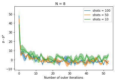
(a)

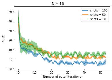
(b)

(c)

Figure 1: Convergence of iVQAGF for three randomly generated MaxCut-SDP instances with different number of vertices in the graph: $N\in\{8,16,32\}$.

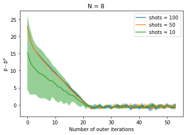
(a)

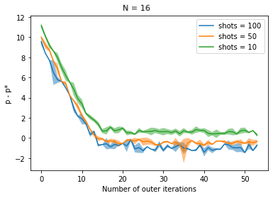
(b)

(c)

Figure 2: Convergence of iVQAEC for three separate cases of randomly generated equality constrained semidefinite programs and nonempty feasbile regions: $N\in\{8,16,32\}$.

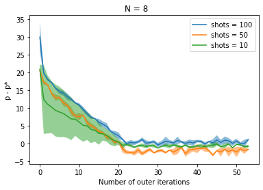
(a)

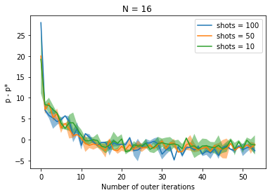
(b)

(c)

Figure 3: Convergence of iVQAIC for three separate cases of randomly generated inequality constrained semidefinite programs with nonempty feasbile regions: $N\in\{8,16,32\}$.

The shaded regions in Figure 1, 2, and 3 signify the variance in the values for different runs (specifically 20) of the algorithm. The $y$-axis measures the difference between the cost function value at each iteration and the actual optimal value evaluated with the CVXPY package. The $x$-axis shows the number of outer iterations of algorithms, i.e., the time needed to converge to the actual optimal value. Lastly, given that the QASM simulator mimics a real quantum device, we specify the number of measurement shots for each run. For our simulations, we run the algorithms for solving an instance of a given randomly generated SDP for three different shots settings: 10, 50, and 100 shots.

The numerical simulations demonstrate that all three algorithms indeed converge to their respective optimal values approximately, even with fewer shots. This numerical evidence suggests that all three proposed algorithms work well in practice.

5 Conclusion

In this paper, we have proposed variational quantum algorithms for solving semidefinite programs. We have considered three constrained formulations of SDPs, which were first converted to unconstrained forms by employing a series of reductions. When the dimension $N$ of the input Hermitian operators of SDPs is large and for these unconstrained forms, the computation of the objective function’s gradient is difficult when using known classical techniques. To overcome this problem, we have utilized parameterized quantum circuits to estimate these gradients. We have also established the convergence rate and total iteration complexity of one of our proposed VQAs. Finally, we have numerically simulated our variational quantum algorithms for different instances of SDPs, and the results of these simulations provide evidence that convergence still occurs in noisy settings.

The estimation of the gradients using parameterized quantum circuits is stochastic in nature. In this paper, we have assumed that we have unbiased estimators of these gradients, and the variance of these estimators is also small. Therefore, it remains open to study the effect of the variance of these estimators on the convergence rate of our algorithms.

Appendix A Appendix

A.1 Proof of Lemma 7

The proof is rather straightforward. First, let us consider a function with two parameters $x$ and $y$, so that $f:\mathbb{R}^{2}\rightarrow\mathbb{R}$. Suppose that the function $(\cdot)\to f(\cdot,y)$ is Lipschitz continuous with Lipschitz constant $L_{X}$, for all $y\in\mathbb{R}$, and suppose that the function $(\cdot)\to f(x,\cdot)$ is Lipschitz continuous with Lipschitz constant $L_{Y}$, for all $x\in\mathbb{R}$. Therefore, the following holds according to the definition of Lipschitz continuity (recall Definition 6):

$$\left|f(x,y)-f(x^{\prime},y)\right| \leq L_{X}\left|x-x^{\prime}\right|\quad\forall x,x^{\prime},y\in\mathbb{R},$$ (95)

$$\left|f(x,y)-f(x,y^{\prime})\right| \leq L_{Y}\left|y-y^{\prime}\right|\quad\forall x,y,y^{\prime}\in\mathbb{R}.$$ (96)

Now consider the following:

$$\left|f(x,y)-f(x^{\prime},y^{\prime})\right| =\left|f(x,y)-f(x^{\prime},y)+f(x^{\prime},y)-f(x^{\prime},y^{\prime})\right|$$ (97)

$$\overset{\mathrm{(a)}}{\leq}\left|f(x,y)-f(x^{\prime},y)\right|+\left|f(x^{\prime},y)-f(x^{\prime},y^{\prime})\right|$$

$$\overset{\mathrm{(b)}}{\leq}L_{X}\left|x-x^{\prime}\right|+L_{Y}\left|y-y^{\prime}\right|$$

$$\leq\max\{L_{X},L_{Y}\}\left(\left|x-x^{\prime}\right|+\left|y-y^{\prime}\right|\right)$$

$$\overset{\mathrm{(c)}}{\leq}\sqrt{2}\max\{L_{X},L_{Y}\}\left\|(x,y)-(x^{\prime},y^{\prime})\right\|,$$

where the inequality $(a)$ follows from the triangle inequality, inequality $(b)$ follows from (95)–(96), and the last inequality $(c)$ follows from the fact that $\left\|\cdot\right\|_{1}\leq\sqrt{2}\left\|\cdot\right\|$. Therefore, $L=\sqrt{2}\max\{L_{x},L_{y}\}$ is a Lipschitz constant for $f$.

The proof given above for two variables can be easily extended to a function $f$ with an $n$-variable input, where $L=\sqrt{n}\max_{i}\{L_{i}\}_{i}$ is a Lipschitz constant given in terms of

$$L_{i}=\sup_{\bm{x}}\left|\frac{\partial f(\bm{x})}{\partial x_{i}}\right|.$$ (98)

Here, $\bm{x}=(x_{1},\ldots,x_{n})^{\top}$.

A.2 Proof of Lemma 8

By hypothesis, each component $f_{i}$ of the vector-valued function $f:\mathbb{R}^{n}\rightarrow\mathbb{R}^{m}$ is $L_{i}$-Lipschitz continuous. Hence, the following holds for all $\bm{x},\bm{x^{\prime}}\in\mathbb{R}^{n}$ and $i$:

$$\left|f_{i}(\bm{x})-f_{i}(\bm{x^{\prime}})\right|\leq L_{i}\left\|\bm{x}-\bm{x^{\prime}}\right\|.$$ (99)

Now consider the following:

$$\left\|f(\bm{x})-f(\bm{x^{\prime}})\right\|^{2} =\sum_{i=1}^{m}\left|f_{i}(\bm{x})-f_{i}(\bm{x^{\prime}})\right|^{2}$$ (100)

$$\leq\sum_{i=1}^{m}L_{i}^{2}\left\|\bm{x}-\bm{x^{\prime}}\right\|^{2}$$ (101)

$$=\left(\sum_{i=1}^{m}L_{i}^{2}\right)\left\|\bm{x}-\bm{x^{\prime}}\right\|^{2}.$$ (102)

Hence, $L=\sqrt{\sum_{i=1}^{m}L_{i}}$ is a Lipschitz constant for the vector-valued function $f$.

A.3 Proof of Lemma 15

According to Lemma 7, a Lipschitz constant of a multivariate function $h(\bm{\theta})=\langle I\otimes O\rangle_{\bm{\theta}}$ is as follows:

$$L_{h} =\sqrt{r}\max_{i}\left\{\sup_{\bm{\theta}}\left|\frac{\partial h(\bm{\theta})}{\partial\theta_{i}}\right|\right\}_{i}$$ (103)

$$\overset{\mathrm{(a)}}{=}\sqrt{r}\max_{i}\left\{\sup_{\bm{\theta}}\left|2\operatorname{Re}\Bigg{[}\langle\bm{0}|U^{\dagger}(\bm{\theta})(I\otimes O)\frac{\partial U(\bm{\theta})}{\partial\theta_{i}}|\bm{0}\rangle\Bigg{]}\right|\right\}_{i}$$

$$\overset{\mathrm{(b)}}{\leq}2\sqrt{r}\max_{i}\left\{\sup_{\bm{\theta}}\left|\langle\bm{0}|U^{\dagger}(\bm{\theta})(I\otimes O)U_{f}(\bm{\theta})e^{-i\theta_{i}H_{i}}(-iH_{i})U_{b}(\bm{\theta})|\bm{0}\rangle\right|\right\}_{i}$$

$$\overset{\mathrm{(c)}}{\leq}2\sqrt{r}\max_{i}\left\{\sup_{\bm{\theta}}\left\|U^{\dagger}(\bm{\theta})(I\otimes O)U_{f}(\bm{\theta})e^{-i\theta_{i}H_{i}}(-iH_{i})U_{b}(\bm{\theta})\right\|\right\}_{i}$$

$$\overset{\mathrm{(d)}}{\leq}2\sqrt{r}\max_{i}\left\{\sup_{\bm{\theta}}\left\|U^{\dagger}(\bm{\theta})\right\|\left\|O\right\|\left\|U_{f}(\bm{\theta})\right\|\left\|e^{-i\theta_{i}H_{i}}\right\|\left\|-iH_{i}\right\|\left\|U_{b}(\bm{\theta})\right\|\right\}_{i}$$

$$\overset{\mathrm{(e)}}{\leq}2\sqrt{r}\left\|O\right\|\max_{i}\left\{\left\|H_{i}\right\|\right\}_{i}.$$

Here, equality (a) is a consequence of the following fact:

$$\frac{\partial h(\bm{\theta})}{\partial\theta_{i}}=\langle\bm{0}|U^{\dagger}(\bm{\theta})(I\otimes O)\frac{\partial U(\bm{\theta})}{\partial\theta_{i}}|\bm{0}\rangle+\langle\bm{0}|\frac{\partial U^{\dagger}(\bm{\theta})}{\partial\theta_{i}}(I\otimes O)U(\bm{\theta})|\bm{0}\rangle,$$ (104)

where we used the chain rule. Inequality (b) follows from the fact that $\left|\operatorname{Re}[z]\right|\leq\left|z\right|$ for all $z\in\mathbb{C}$ . Additionally, we assume $U(\bm{\theta})=U_{f}(\bm{\theta})e^{-i\theta_{i}H_{i}}U_{b}(\bm{\theta})$, so that

$$\frac{\partial U(\bm{\theta})}{\partial\theta_{i}}=U_{f}(\bm{\theta})e^{-i\theta_{i}H_{i}}(-iH_{i})U_{b}(\bm{\theta}).$$ (105)

Inequality (c) follows from the fact that $\left\|A\right\|=\sup_{|\psi\rangle,|\phi\rangle}\{|\langle\psi|A|\phi\rangle|:\left\||\psi\rangle\right\|=\left\||\phi\rangle\right\|=1\}$. Inequality (d) follows from two properties of the spectral norm of a matrix: $\ \|AB\|\leq\|A\|\|B\|$ and $\|A\otimes B\|\leq\|A\|\|B\|$. The inequality $(e)$ follows from the fact that $\|V\|=1$ for every unitary $V$.

A.4 Proof of Lemma 16

A multivariate vector-valued function $\nabla_{\bm{\theta}}\mathcal{L}_{c}(\bm{\theta},\bm{y})$ is $L_{c,\bm{y}}$-Lipschitz continuous for a fixed $\bm{y}\in\mathbb{R}^{M}$ if all its components, i.e., $\left\{\frac{\partial\mathcal{L}_{c}(\bm{\theta},\bm{y})}{\partial\theta_{i}}\right\}_{i=1}^{r}$, are Lipschitz continuous for a fixed $\bm{y}\in\mathbb{R}^{M}$. In order to prove that $\frac{\partial\mathcal{L}_{c}(\bm{\theta},\bm{y})}{\partial\theta_{i}}$ is $L_{c,\bm{y}}^{i}$-Lipschitz continuous, we need to bound the Lipschitz constant $L_{c,\bm{y}}^{i}$ from above. According to Lemma 7, we state the following:

$$L_{c,\bm{y}}^{i} =\sqrt{r}\max_{j}\left\{\sup_{\bm{\theta}}\left|\frac{\partial^{2}\mathcal{L}_{c}(\bm{\theta},\bm{y})}{\partial\theta_{i}\partial\theta_{j}}\right|\right\}_{j}$$ (106)

$$\leq\sqrt{r}\max_{j}\Bigg{\{}\sup_{\bm{\theta}}\Bigg{\{}\lambda\left|\frac{\partial^{2}\langle I\otimes C\rangle_{\bm{\theta}}}{\partial\theta_{i}\partial\theta_{j}}\right|+\lambda\sum_{m=1}^{M}\left|y_{m}\right|\left|\frac{\partial^{2}\langle I\otimes A_{m}\rangle_{\bm{\theta}}}{\partial\theta_{i}\partial\theta_{j}}\right|$$

$$\qquad\qquad\qquad\qquad+\lambda c\sum_{m=1}^{M}\Bigg{(}\left|b_{m}\right|\left|\frac{\partial^{2}\langle I\otimes A_{m}\rangle_{\bm{\theta}}}{\partial\theta_{i}\partial\theta_{j}}\right|+\lambda\left|\langle I\otimes A_{m}\rangle_{\bm{\theta}}\right|\left|\frac{\partial^{2}\langle I\otimes A_{m}\rangle_{\bm{\theta}}}{\partial\theta_{i}\partial\theta_{j}}\right|$$

$$\qquad\qquad\qquad\qquad\qquad+\lambda\left|\frac{\partial\langle I\otimes A_{m}\rangle_{\bm{\theta}}}{\partial\theta_{i}}\right|\left|\frac{\partial\langle I\otimes A_{m}\rangle_{\bm{\theta}}}{\partial\theta_{j}}\right|\Bigg{)}\Bigg{\}}\Bigg{\}}_{j},$$

where $j\in\{1,\ldots,r\}$, and the aforementioned inequality follows from the triangle inequality. Let us first bound $\sup_{\bm{\theta}}\left|\frac{\partial^{2}\langle I\otimes O\rangle_{\bm{\theta}}}{\partial\theta_{i}\partial\theta_{j}}\right|$ from above as follows, where $O\in\{C,A_{1},\dots,A_{M}\}$:

$$\sup_{\bm{\theta}}\left|\frac{\partial^{2}\langle I\otimes O\rangle_{\bm{\theta}}}{\partial\theta_{i}\partial\theta_{j}}\right|$$ (107)

$$\overset{\mathrm{(a)}}{=}\sup_{\bm{\theta}}\left\{\left|2\operatorname{Re}\Bigg{[}\langle\bm{0}|U^{\dagger}(\bm{\theta})(I\otimes O)\frac{\partial^{2}U(\bm{\theta})}{\partial\theta_{i}\partial\theta_{j}}|\bm{0}\rangle\Bigg{]}+2\operatorname{Re}\Bigg{[}\langle\bm{0}|\frac{\partial U^{\dagger}(\bm{\theta})}{\partial\theta_{i}}(I\otimes O)\frac{\partial U(\bm{\theta})}{\partial\theta_{j}}|\bm{0}\rangle\Bigg{]}\right|\right\}$$

$$\overset{\mathrm{(b)}}{\leq}2\sup_{\bm{\theta}}\left\{\left|\operatorname{Re}\Bigg{[}\langle\bm{0}|U^{\dagger}(\bm{\theta})(I\otimes O)\frac{\partial^{2}U(\bm{\theta})}{\partial\theta_{i}\partial\theta_{j}}|\bm{0}\rangle\Bigg{]}\right|+\left|\operatorname{Re}\Bigg{[}\langle\bm{0}|\frac{\partial U^{\dagger}(\bm{\theta})}{\partial\theta_{i}}(I\otimes O)\frac{\partial U(\bm{\theta})}{\partial\theta_{j}}|\bm{0}\rangle\Bigg{]}\right|\right\}$$

$$\overset{\mathrm{(c)}}{\leq}2\sup_{\bm{\theta}}\Bigg{\{}\left|\langle\bm{0}|U^{\dagger}(\bm{\theta})(I\otimes O)U_{ff}(\bm{\theta})e^{-i\theta_{j}H_{j}}(-iH_{j})U_{fb}(\bm{\theta})e^{-i\theta_{i}H_{i}}(-iH_{i})U_{b}(\bm{\theta})|\bm{0}\rangle\right|$$

$$\qquad\qquad\qquad+\left|\langle\bm{0}|U_{b}^{\dagger}(\bm{\theta})e^{i\theta_{i}H_{i}}(iH_{i})U_{f}^{\dagger}(\bm{\theta})(I\otimes O)U_{ff}(\bm{\theta})e^{-i\theta_{j}H_{j}}(-iH_{j})U_{b^{\prime}}(\bm{\theta})|\bm{0}\rangle\right|\Bigg{\}}$$

$$\overset{\mathrm{(d)}}{\leq}4\left\|O\right\|\left\|H_{j}\right\|\left\|H_{i}\right\|,$$ (108)

where equality (a) follows from the chain rule applied twice (see (104)). Inequality (b) follows from the triangle inequality. Inequality (c) follows from the fact that $\left|\operatorname{Re}[z]\right|\leq\left|z\right|$ for all $z\in\mathbb{C}$, as well as from the assumption that $U(\bm{\theta})$ has the following decomposition:

$$U(\bm{\theta})=U_{ff}(\bm{\theta})e^{-i\theta_{j}H_{j}}U_{fb}(\bm{\theta})e^{-i\theta_{i}H_{i}}U_{b}(\bm{\theta}).$$ (109)

Additionally, let $U_{ff}(\bm{\theta})e^{-i\theta_{j}H_{j}}U_{fb}(\bm{\theta})=U_{f}(\bm{\theta})$ and $U_{fb}(\bm{\theta})e^{-i\theta_{i}H_{i}}U_{b}(\bm{\theta})=U_{b^{\prime}}(\bm{\theta})$. Inequality (d) follows from a set of arguments similar to those in the proof of Lemma 15.

Second, we bound $\sup_{\bm{\theta}}\left|\langle I\otimes O\rangle_{\bm{\theta}}\right|$ from above as follows, where $O\in\{A_{1},\dots,A_{M}\}$:

$$\sup_{\bm{\theta}}\left|\langle I\otimes O\rangle_{\bm{\theta}}\right| =\sup_{\bm{\theta}}\left|\langle\bm{0}|U^{\dagger}(\bm{\theta})(I\otimes O)U(\bm{\theta})|\bm{0}\rangle\right|$$ (110)

$$\leq\left\|O\right\|.$$ (111)

Finally, we bound $\sup_{\bm{\theta}}\left|\frac{\partial\langle I\otimes O\rangle_{\bm{\theta}}}{\partial\theta_{i}}\right|$ from above as follows, where $O\in\{A_{1},\dots,A_{M}\}$:

$$\sup_{\bm{\theta}}\left|\frac{\partial\langle I\otimes O\rangle_{\bm{\theta}}}{\partial\theta_{i}}\right| =\sup_{\bm{\theta}}\left|2\operatorname{Re}\Bigg{[}\langle\bm{0}|U^{\dagger}(\bm{\theta})(I\otimes O)\frac{\partial U(\bm{\theta})}{\partial\theta_{i}}|\bm{0}\rangle\Bigg{]}\right|$$ (112)

$$\leq 2\left\|O\right\|\left\|H_{i}\right\|.$$ (113)

The above inequality follows from the similar set of arguments made in the proof of Lemma 15.

Note that the upper bounds in (108), (111), and (113) are independent of $\bm{\theta}$. Hence, using these upper bounds, we bound $L_{c,\bm{y}}^{i}$ from above as follows:

$$L_{c,\bm{y}}^{i} \leq\sqrt{r}\max_{j}\Bigg{\{}4\lambda\left\|C\right\|\left\|H_{j}\right\|\left\|H_{i}\right\|+\lambda\sum_{m=1}^{M}4\left|y_{m}\right|\left\|A_{m}\right\|\left\|H_{j}\right\|\left\|H_{i}\right\|$$ (114)

$$\quad\quad+\lambda c\sum_{m=1}^{M}\left(4\left|b_{m}\right|\left\|A_{m}\right\|\left\|H_{j}\right\|\left\|H_{i}\right\|+4\lambda\left\|A_{m}\right\|^{2}\left\|H_{j}\right\|\left\|H_{i}\right\|+4\lambda\left\|A_{m}\right\|^{2}\left\|H_{j}\right\|\left\|H_{i}\right\|\right)\Bigg{\}}_{j}$$

$$=4\lambda\sqrt{r}\left\|H_{i}\right\|\left(\left\|C\right\|+\sum_{m=1}^{M}\left(\left(\left|y_{m}\right|+c\left|b_{m}\right|\right)\left\|A_{m}\right\|+2c\lambda\left\|A_{m}\right\|^{2}\right)\right)\max_{j}\left\{\left\|H_{j}\right\|\right\}_{j}$$ (115)

From (115) we conclude that the Lipschitz constant $L_{c,\bm{y}}^{i}$ is bounded from above by a positive number. Hence, the Lipschitz constant $L_{c,\bm{y}}$ of $\nabla_{\bm{\theta}}\mathcal{L}_{c}(\bm{\theta})$ is also bounded from above by a positive number because $L_{c,\bm{y}}=\sqrt{\sum_{i=1}^{r}L_{c,\bm{y}}^{i}}$ according to Lemma 8. Thus, the function $\mathcal{L}_{c}(\bm{\theta},\bm{y})$ is $L_{c,\bm{y}}$-smooth for a fixed $\bm{y}\in\mathbb{R}^{M}$.

A.5 Proof of Lemma 20

A multivariate vector-valued function $\nabla_{\bm{\theta}}\mathcal{F}_{\gamma}(\bm{\theta},\bar{\bm{y}})$ for a fixed $\bar{\bm{y}}\geq 0$, is $L_{\gamma,\bar{\bm{y}}}$-Lipschitz continuous if all its components, i.e., $\left\{\frac{\partial\mathcal{F}_{\gamma}(\bm{\theta},\bar{\bm{y}})}{\partial\theta_{i}}\right\}_{i=1}^{r}$, are Lipschitz continuous for a fixed $\bar{\bm{y}}\geq 0$. In order to prove that $\frac{\partial\mathcal{F}_{\gamma}(\bm{\theta},\bar{\bm{y}})}{\partial\theta_{i}}$ is $L_{\gamma,\bar{\bm{y}}}^{i}$-Lipschitz continuous, we first bound the Lipschitz constant $L_{\gamma,\bar{\bm{y}}}^{i}$ from above as follows:

$$L_{\gamma,\bar{\bm{y}}}^{i} =\sqrt{r}\max_{j}\left\{\sup_{\bm{\theta}}\left|\frac{\partial^{2}\mathcal{F}_{\gamma}(\bm{\theta},\bar{\bm{y}})}{\partial\theta_{i}\partial\theta_{j}}\right|\right\}_{j}$$ (116)

$$\begin{split}&=b_{M}\sqrt{r}\max_{j}\Bigg{\{}\sup_{\bm{\theta}}\Bigg{|}\frac{e^{\gamma\langle I\otimes H(\bar{\bm{y}})\rangle_{\bm{\theta}}}}{\left(e^{\gamma\langle I\otimes H(\bar{\bm{y}})\rangle_{\bm{\theta}}}+1\right)}\frac{\partial^{2}\langle I\otimes H(\bar{\bm{y}})\rangle_{\bm{\theta}}}{\partial\theta_{i}\partial\theta_{j}}\\ &\qquad\qquad\qquad\qquad\qquad+\frac{e^{\gamma\langle I\otimes H(\bar{\bm{y}})\rangle_{\bm{\theta}}}}{\left(e^{2\gamma\langle I\otimes H(\bar{\bm{y}})\rangle_{\bm{\theta}}}+1\right)}\gamma\frac{\partial\langle I\otimes H(\bar{\bm{y}})\rangle_{\bm{\theta}}}{\partial\theta_{i}}\frac{\partial\langle I\otimes H(\bar{\bm{y}})\rangle_{\bm{\theta}}}{\partial\theta_{j}}\Bigg{|}\Bigg{\}}_{j}\end{split}$$

$$\leq b_{M}\sqrt{r}\max_{j}\left\{\sup_{\bm{\theta}}\left|\frac{\partial^{2}\langle I\otimes H(\bar{\bm{y}})\rangle_{\bm{\theta}}}{\partial\theta_{i}\partial\theta_{j}}+\gamma\frac{\partial\langle I\otimes H(\bar{\bm{y}})\rangle_{\bm{\theta}}}{\partial\theta_{i}}\frac{\partial\langle I\otimes H(\bar{\bm{y}})\rangle_{\bm{\theta}}}{\partial\theta_{j}}\right|\right\}_{j}$$

$$\leq b_{M}\sqrt{r}\max_{j}\left\{\sup_{\bm{\theta}}\left|\frac{\partial^{2}\langle I\otimes H(\bar{\bm{y}})\rangle_{\bm{\theta}}}{\partial\theta_{i}\partial\theta_{j}}\right|+\gamma\left|\frac{\partial\langle I\otimes H(\bar{\bm{y}})\rangle_{\bm{\theta}}}{\partial\theta_{i}}\right|\left|\frac{\partial\langle I\otimes H(\bar{\bm{y}})\rangle_{\bm{\theta}}}{\partial\theta_{j}}\right|\right\}_{j}$$

$$\leq 4b_{M}\sqrt{r}\left\|H_{i}\right\|\left(\left\|H(\bar{\bm{y}})\right\|+4\gamma\left\|H(\bar{\bm{y}})\right\|^{2}\right)\max_{j}\left\{\left\|H_{j}\right\|\right\}_{j}.$$

The last inequality follows from (113) and (108). We see that $L_{\gamma,\bar{\bm{y}}}^{i}$ is bounded from above by a positive number for a fixed $\bar{\bm{y}}$. Therefore, the Lipschitz constant $L_{\gamma,\bar{\bm{y}}}$ is also bounded from above by a positve number because according to Lemma 8, we have $L_{\gamma,\bar{\bm{y}}}=\sqrt{\sum_{i=1}^{r}L_{\gamma,\bar{\bm{y}}}^{i}}$. Thus, function $\mathcal{F}_{\gamma}(\bm{\theta},\bar{\bm{y}})$ is $L_{\gamma,\bar{\bm{y}}}$-smooth for a fixed $\bar{\bm{y}}\geq 0$.

References

- [AAA+21] M. D. Sajid Anis, Héctor Abraham, AduOffei, Rochisha Agarwal, et al. Qiskit: An open-source framework for quantum computing, 2021.
- [AAB+19] Frank Arute, Kunal Arya, Ryan Babbush, et al. Quantum supremacy using a programmable superconducting processor. Nature, 574:505–510, October 2019.
- [AK16] Sanjeev Arora and Satyen Kale. A combinatorial, primal-dual approach to semidefinite programs. Journal of the ACM, 63(2):1–35, May 2016.
- [BCLK+21] Kishor Bharti, Alba Cervera-Lierta, Thi Ha Kyaw, Tobias Haug, Sumner Alperin-Lea, Abhinav Anand, Matthias Degroote, Hermanni Heimonen, Jakob S. Kottmann, Tim Menke, Wai-Keong Mok, Sukin Sim, Leong-Chuan Kwek, and Alán Aspuru-Guzik. Noisy intermediate-scale quantum (NISQ) algorithms. January 2021. arXiv:2101.08448.
- [BHVK21] Kishor Bharti, Tobias Haug, Vlatko Vedral, and Leong-Chuan Kwek. Nisq algorithm for semidefinite programming, 2021. arXiv:2106.03891.
- [BKL+19] Fernando G. S. L. Brandão, Amir Kalev, Tongyang Li, Cedric Yen-Yu Lin, Krysta M. Svore, and Xiaodi Wu. Quantum SDP solvers: Large speed-ups, optimality, and applications to quantum learning. In 46th International Colloquium on Automata, Languages, and Programming, ICALP 2019, July 9-12, 2019, Patras, Greece, volume 132 of LIPIcs, pages 27:1–27:14. Schloss Dagstuhl - Leibniz-Zentrum für Informatik, 2019.
- [BS17] Fernando G. S. L. Brandão and Krysta M. Svore. Quantum speed-ups for solving semidefinite programs. In 2017 IEEE 58th Annual Symposium on Foundations of Computer Science (FOCS), pages 415–426. IEEE Computer Society, October 2017.
- [BV04] Stephen P. Boyd and Lieven Vandenberghe. Convex Optimization. Cambridge University Press, March 2004.
- [CAB+21] Marco Cerezo, Andrew Arrasmith, Ryan Babbush, Simon Benjamin, Suguro Endo, Keisuke Fujii, Jarrod Ryan McClean, Kosuke Mitarai, Xiao Yuan, Lukasz Cincio, and Patrick Coles. Variational quantum algorithms. Nature Reviews Physics, 3:625–644, September 2021.
- [DH96] Christoph Dürr and Peter Høyer. A quantum algorithm for finding the minimum. July 1996. arXiv:quant-ph/9607014.
- [dKRT95] Etienne de Klerk, Cornelis Roos, and Tamás Terlaky. Semi-definite problems in truss topology optimization. Delft University of Technology, Faculty of Technical Mathematics and Informatics, 1995. https://www.academia.edu/17783851/Semi_definite_problems_in_truss_topology_optimization.
- [Eld03] Yonina C. Eldar. A semidefinite programming approach to optimal unambiguous discrimination of quantum states. IEEE Transactions on Information Theory, 49(2):446–456, February 2003.
- [FGG14] Edward Farhi, Jeffrey Goldstone, and Sam Gutmann. A quantum approximate optimization algorithm, November 2014. arXiv:1411.4028.
- [Gro97] Lov K. Grover. Quantum mechanics helps in searching for a needle in a haystack. Physical Review Letters, 79(2):325–328, July 1997.
- [GW95] Michel X. Goemans and David P. Williamson. Improved approximation algorithms for maximum cut and satisfiability problems using semidefinite programming. Journal of the ACM, 42(6):1115–1145, November 1995.
- [HD21] Patrick Huembeli and Alexandre Dauphin. Characterizing the loss landscape of variational quantum circuits. Quantum Science and Technology, 6(2):025011, February 2021.
- [Hes69] Magnus R. Hestenes. Multiplier and gradient methods. Journal of Optimization Theory and Applications, 4(5):303–320, November 1969.
- [HHL09] Aram W. Harrow, Avinatan Hassidim, and Seth Lloyd. Quantum algorithm for linear systems of equations. Physical Review Letters, 103(15):150502, October 2009.
- [HV03] Ramesh Hariharan and Vishwanathan Vinay. String matching in quantum time. Journal of Discrete Algorithms, 1(1):103–110, November 2003.
- [HWBT15] Matthew B. Hastings, Dave Wecker, Bela Bauer, and Matthias Troyer. Improving quantum algorithms for quantum chemistry. Quantum Information and Computation, 15(1–2):1–21, January 2015.
- [KE95] James Kennedy and Russell Eberhart. Particle swarm optimization. In Proceedings of ICNN’95-international conference on neural networks, volume 4, pages 1942–1948. IEEE, November 1995.
- [KNS16] Hamed Karimi, Julie Nutini, and Mark Schmidt. Linear convergence of gradient and proximal-gradient methods under the Polyak-Lojasiewicz condition. In Machine Learning and Knowledge Discovery in Databases, pages 795–811. Springer, Cham, Switzerland, September 2016.
- [LL15] Huan Li and Zhouchen Lin. Accelerated proximal gradient methods for nonconvex programming. In NIPS’15: Proceedings of the 28th International Conference on Neural Information Processing Systems - Volume 1, pages 379–387. MIT Press, Cambridge, MA, USA, December 2015.
- [LS06] László Lovász and Alexander Schrijver. Cones of matrices and set-functions and 0-1 optimization. Society for Industrial and Applied Mathematics Journal on Optimization, 1(2):166–190, July 2006.
- [MP90] Bojan Mohar and Svatopluk Poljak. Eigenvalues and the max-cut problem. Czechoslovak Mathematical Journal, 40(2):343–352, 1990.
- [NM65] John A Nelder and Roger Mead. A simplex method for function minimization. The computer journal, 7(4):308–313, January 1965.
- [Par03] Pablo A. Parrilo. Semidefinite programming relaxations for semialgebraic problems. Mathematical Programming, 96(2):293–320, 2003.
- [PMS+14] Alberto Peruzzo, Jarrod McClean, Peter Shadbolt, Man-Hong Yung, Xiao-Qi Zhou, Peter J. Love, Alán Aspuru-Guzik, and Jeremy L. O’Brien. A variational eigenvalue solver on a photonic quantum processor. Nature Communications, 5:4213, July 2014.
- [Pow69] Michael J. D. Powell. A method for nonlinear constraints in minimization problems. Optimization, pages 283–298, 1969.
- [Pre18] John Preskill. Quantum computing in the NISQ era and beyond. Quantum, 2:79, August 2018.
- [PW00] Florian A. Potra and Stephen J. Wright. Interior-point methods. Journal of Computational and Applied Mathematics, 124(1):281–302, December 2000.
- [PY91] Christos H. Papadimitriou and Mihalis Yannakakis. Optimization, approximation, and complexity classes. Journal of Computer and System Sciences, 43(3):425–440, December 1991.
- [PZ03] John Proos and Christof Zalka. Shor’s discrete logarithm quantum algorithm for elliptic curves. Quantum Information and Computation, 3(4):317–344, July 2003.
- [S+92] James C Spall et al. Multivariate stochastic approximation using a simultaneous perturbation gradient approximation. IEEE transactions on automatic control, 37(3):332–341, March 1992.
- [SB20] Ivan Supic and Joseph Bowles. Self-testing of quantum systems: a review. Quantum, 4:337, September 2020.
- [SBG+19] Maria Schuld, Ville Bergholm, Christian Gogolin, Josh Izaac, and Nathan Killoran. Evaluating analytic gradients on quantum hardware. Physical Review A, 99(3):032331, March 2019.
- [SEA+19] Mehmet Fatih Sahin, Armin Eftekhari, Ahmet Alacaoglu, Fabian Latorre Gómez, and Volkan Cevher. An inexact augmented Lagrangian framework for nonconvex optimization with nonlinear constraints. In Advances in Neural Information Processing Systems 32: Annual Conference on Neural Information Processing Systems 2019, NeurIPS 2019, December 8-14, 2019, Vancouver, BC, Canada, pages 13943–13955, 2019.
- [Sho94] Peter W. Shor. Algorithms for quantum computation: Discrete logarithms and factoring. In 35th Annual Symposium on Foundations of Computer Science, pages 124–134, Santa Fe, New Mexico, USA, November 1994. IEEE Computer Society.
- [Sio58] Maurice Sion. On general minimax theorems. Pacific Journal of Mathematics, 8(1):171–176, March 1958.
- [vAGGdW20] Joran van Apeldoorn, András Gilyén, Sander Gribling, and Ronald de Wolf. Quantum SDP-solvers: Better upper and lower bounds. Quantum, 4:230, February 2020.
- [Wan18] Xin Wang. Semidefinite optimization for quantum information. PhD thesis, University of Technology Sydney, Centre for Quantum Software and Information, Faculty of Engineering and Information Technology, July 2018. http://hdl.handle.net/10453/127996.
- [Wat18] John Watrous. The Theory of Quantum Information. Cambridge University Press, 2018.
- [WXD18] Xin Wang, Wei Xie, and Runyao Duan. Semidefinite programming strong converse bounds for classical capacity. IEEE Transactions on Information Theory, 64(1):640–653, January 2018.
- [YKL75] Horace Yuen, Robert Kennedy, and Melvin Lax. Optimum testing of multiple hypotheses in quantum detection theory. IEEE Transactions on Information Theory, 21(2):125–134, March 1975.