The relativistic parsec-scale jets of the blazars TXS 0506+056 and PKS 0502+049 and their possible association with gamma-ray flares and neutrino production

Abstract

The physical nature of the mechanism responsible for the emission of neutrinos in active galactic nuclei (AGN) has been matter of debate in the literature, with relativistic jets of radio-loud AGNs as possible candidates to be the sources of high energy neutrinos. The most prominent candidate so far is the blazar TXS 0506+056, which is found to be associated with the neutrino event IceCube-170922A. Furthermore, the IceCube reported an excess of neutrinos towards TXS 0506+056 between September 2014 and March 2015, even though this association needs additional investigation, considering the presence of a nearby $\gamma$-ray source, the quasar PKS 0502+049. Motivated by this, we studied the parsec-scale structures of TXS 0506+056 and PKS 0502+049 through radio interferometry at 8 and 15 GHz. We identified twelve jet components in TXS 0506+056 and seven components in PKS 0502+049. The most reliable jet components show superluminal speeds ranging from $9.5c$ to $66c$ in the case of TXS 0506+056, and from $14.3c$ to $59c$ for PKS 0502+049, which were used to estimate a lower (upper) limit for the Lorentz factor (jet viewing angle) for both sources. A novel approach using simultaneously the brightness temperature of the core region and the apparent speeds of the jet components allowed us to infer basic jet parameters for TXS 0506+056 at distinct epochs. We also found that the emergence of new jet components coincides with the occurrence of gamma-ray flares. Interestingly, two of these coincidences in the case of PKS 0502+049 and one for TXS 0506+056 seems to be correlated with neutrino events detected by the IceCube Observatory.

1 Introduction

Blazars are a subclass of active galaxies whose jets form a small angle with respect to our line of sight and usually exhibit strong variability from radio up to TeV gamma-rays, presenting a non-thermal continuum and a relativistic jet (e.g., Urry & Padovani, 1995). They have also been considered powerful cosmic particle accelerators and thus prominent candidates of high-energy (HE) astrophysical neutrinos generated in hadronic interactions in their jets (e.g., Stecker et al., 1991; Mannheim, 1995; Gao et al., 2017; Murase, 2017; Rodrigues et al., 2018; Murase et al., 2018).

Located at a redshift of $0.3356$ (Paiano et al., 2018), the BL Lac object TXS 0506+056 was recently proposed as the object that produced the 290 TeV muon neutrino related to the IceCube-170922A detection (IceCube Collaboration et al., 2018). This event has opened new perspectives for investigating the multi-messenger physics of blazars jets. Moreover, motivated by this HE neutrino detection and after an archival search, the IceCube collaboration reported a 3.5 $\sigma$ excess of neutrinos from the direction of TXS 0506+056, with energy above 30 TeV, during a time window from September 2014 to March 2015 (IceCube Collaboration, 2018). The interpretation of such events turned out to be a difficult task, since the source TXS 0506+056 was in a quiescent state of both the radio and gamma-ray emission during this period (Liang et al., 2018; Padovani et al., 2018).

The flat spectrum radio quasar (FSRQ) PKS 0502+049 is separated by an angular distance of $1\aas@@fstack{\circ}2$ from TXS 0506+056 (Johnston et al., 1995). At a redshift of 0.954 (Drinkwater et al., 1997), PKS 0502+049 was identified as a GeV gamma-ray emitter just before and immediately after the period of the neutrino excess in 2014-2015 (He et al., 2018), so its contribution may not be disregarded.

Different mechanisms responsible for the production of these detected neutrinos and gamma-rays from both blazars have been proposed in the literature (e.g., Ansoldi et al., 2018; He et al., 2018; Sahakyan, 2018, 2019; Rodrigues et al., 2019; Liu et al., 2019; Banik & Bhadra, 2019; Banik et al., 2020). However, the results remain controversial.

Some groups have studied the kinematics of the parsec-scale jet of TXS 0506+056 using the standard Difmap tasks (Shepherd, 1997) to model the sky brightness distribution for VLBA observations in the $(u,v)$ visibility plane. Kun et al. (2019), Lister et al. (2019), and Li et al. (2020) identified four peculiar features which maintain quasi-stationary separations from the core, in a region extending up to 4 mas. On the other hand, Britzen et al. (2019) suggested two scenarios in order to explain the evidence for a strong curvature in the jet of TXS 0506+056. The first scenario is characterised by one strongly curved jet while the second is defined by a structure made up of two jets. None of these studies could provide any temporal correlation between the ejection of the jet components and the HE neutrinos events. In the case of PKS 0502+049, there is no published kinematic study from the best of our knowledge.

The correlated observation of HE neutrinos and enhanced gamma-ray activity with ejection of jet components may shed some light to the production scenario of these detected neutrinos and gamma-rays from the blazars. Thus, the primary objective of this work consists of a kinematic study of the parsec-scale jets of the blazars TXS 0506+056 and PKS 0502+049. We have gathered existing VLBI data of TXS 0506+056 from the MOJAVE/VLBA Survey archive (Lister et al., 2009a) to apply the global optimisation statistical technique Cross-Entropy (hereafter CE; Rubinstein, 1997). Adapted by Caproni et al. (2011), this method allows to model interferometric radio images of astrophysical jets and estimate a minimum number of discrete two-dimensional elliptical Gaussian components at each epoch (e.g., Caproni et al., 2014, 2017). We also investigated kinematically whether the estimated ejection epochs of PKS 0502+049 jet components, which accompany the observed gamma-ray flux, may or may not contribute to the events detected by the IceCube Observatory.

This work is structured as follows: the observational data set used in this work is presented in section 2. The general results from our kinematic studies of the parsec-scale jets of TXS 0506+056 and PKS 0502+049, including a novel approach to estimate the values of some jet parameters are shown in section 3. A possible connection between jet components and neutrino emission are explored in section 4. Final remarks are presented in section 5. We assume throughout this work $H_{0}$ = 71 km s^-1 Mpc^-1, $\Omega_{\mathrm{M}}$ = 0.27 and $\Omega_{\Lambda}$ = 0.73, implying that 1.0 mas = 4.78 pc and 1.0 mas yr^-1 = 20.84$c$ for TXS 0506+056, where $c$ is the speed of light. In the case of PKS 0502+049, 1.0 mas = 7.94 pc and 1.0 mas yr^-1 = 50.63$c$.

2 Data analysis

2.1 Radio interferometric data

We investigate the structure of the parsec-scale jet of TXS 0506+056 and PKS 0502+049 by employing available VLBI data from archival databases. These data consist of naturally weighted total intensity maps obtained at 15 GHz, publicly available at MOJAVE/2-cm Survey Data Archive (Lister et al., 2009a), spanning from 2009 to 2020 and 2016 to 2020 for TXS 0506+056 and PKS 0502+049, respectively. One additional map for PKS 0502+049 was acquired from the Astrogeo Center at 8 GHz in November 2018. In LABEL:table:Characteristics_TXS_table and LABEL:table:Characteristics_PKS_table, we list the main characteristics of these images for TXS 0506+056 and PKS 0502+049, respectively, represented by the peak intensity ($I_{\mathrm{max}}$), the root mean square (RMS) of the off-source surface brightness, and the parameters of the synthesised elliptical clean beam, which are the FWHM major axis ($\Theta^{\mathrm{FWHM}}_{\mathrm{beam}}$), eccentricity ($\epsilon_{\mathrm{\,beam}}$) and position angle ($\theta_{\mathrm{beam}}$) on the plane of the sky.

The FITS images are constituted by an array of $1024\times 1024$ or $512\times 512$ pixels in right ascension and declination directions. For the purpose of minimising the computational time required for our model-fitting algorithm to find the optimal solutions, we cropped the original data to maintain only the fraction with a useful signal (source) without compromising the obtained results .

The radio maps of TXS 0506+056 and PKS 0502+049 reveal a relatively intense radio core and an inconspicuous jet that extends up to 4 mas on one side of the core. The surface brightness of these jets was decomposed in elliptical Gaussian components and their structural parameters were determined via the Cross-Entropy (CE) global optimisation technique (e.g., Rubinstein, 1997; Caproni et al., 2014, 2017). Each elliptical Gaussian component is characterised by six structural parameters: two-dimensional peak position ($x_{0},y_{0}$), with coordinates $x$ and $y$ oriented in right ascension and declination directions, respectively; peak intensity, $I_{0}$, semi-major axis, $a$, eccentricity, $\epsilon=\sqrt{1-(b/a)^{2}}$, where $b$ is the semi-minor axis, and the position angle of the major axis, $\psi$, measured positively from west to north.

Following the criteria proposed in Caproni et al. (2014), we found the optimal number of Gaussian components in each image, leading to a minimum of two and a maximum of six components in the images analysed in this work. The CE model-fitting results of TXS 0506+056 and PKS 0502+049 on four representative epochs at 15 GHz can be seen in Figure 1, in which the Gaussian components are shown superimposed on the observed image, as well as the respective residual maps. These epochs were not chosen at random, we selected interferometric radio observations whose dates preceded or followed the IceCube-170922A event or the 2014-2015 neutrino excess.

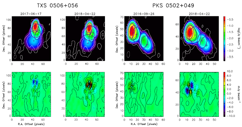
Figure 1: Parsec-scale radio structure of TXS 0506+056 (left panels) and PKS 0502+049 (right panels) at 15 GHz analysed in this work and their respective residual maps. White contour lines depict the VLBA map, while the superimposed dark thick ellipses are the contours of the Gaussian CE model-fitting components at the FWHM (centre marked with crosses). The observation epochs are marked in the top of each panel and refer from left to right, respectively, to: 2017-06-17 - two months before the IceCube-170922A event; 2018-04-22 - seven months after the IceCube-170922A event; 2016-09-26 - corresponding to the first observation epoch of the available archival VLBA data of PKS 0502+049, 1.5 yr after the 2014-2015 neutrino excess; 2018-04-22 - seven months after the IceCube-170922A event. The ellipse in the lower-left corner of the individual panels represents the FWHM of the elliptical synthesised clean beam.

The structural parameters of the Gaussian components derived by our CE optimisations are listed in Tables LABEL:table:Parameters_TXS_table, LABEL:table:Parameters_PKS_15GHz_table and LABEL:table:Parameters_PKS_8GHz_table. The flux density, $F$, (the entries in the third column of these tables) was estimated from

$$F=8\ln{2}\left[\frac{a^{2}\sqrt{1-\epsilon^{2}}}{\left(\Theta^{\mathrm{FWHM}}_{\mathrm{beam}}\right)^{2}\sqrt{1-\epsilon^{2}_{\mathrm{beam}}}}\right]I_{0}\;.$$ (1)

The formal uncertainties for the elliptical Gaussian parameters were obtained from weighted mean and standard deviation of the best tentative solution at each iteration during the CE optimisations (see Equations 10 and 11 in Caproni et al. 2011). As pointed out in Caproni et al. (2011), these error estimates should be assumed as a lower limit for the true uncertainties of the derived Gaussian parameters. In the case of the uncertainties in the Gaussian peak positions, we also added a term corresponding to 1/10 of the FWHM restoring beam dimensions (e.g., Lister et al. 2009b) in quadrature to the respective CE uncertainties in those quantities (e.g., Caproni et al. 2014), providing more conservative estimates of the errors in the sky positions of the Gaussian components.

The last column of Tables LABEL:table:Parameters_TXS_table, LABEL:table:Parameters_PKS_15GHz_table and LABEL:table:Parameters_PKS_8GHz_table indicates the brightness temperature of the core in the observer’s reference frame, which will be discussed in detail in subsection 3.3.

The jet inlet region, or simply the core component, is the most intense component in terms of flux density found in our CE modellings for both sources, and it is always located at the northernmost part of the analysed interferometric images. The same components detected in the 8-GHz map of PKS 0502+049 are seen in the quasi-contemporaneous image at 15 GHz, reinforcing the robustness of our CE modelling.

2.2 Gamma-ray data

The $\gamma$-ray data analysed in this work was extracted from the public Fermi Large Area Telescope Pass 8 database (Atwood et al., 2009, 2013). A standard Fermi-LAT unbinned likelihood analysis was performed in order to obtain the light curves of PKS 0502+049 and TXS 0506+056 and unveil the association between the emergence of parsec-scale radio components and $\gamma$-ray flares, and also how these light curves are connected to the neutrino events reported by the IceCube Collaboration (IceCube Collaboration, 2018).

The analysed data-set was extracted in the period of the 4th of August 2008 and the 05th of June 2019 and the respective photon energy range was between $300$ MeV$\leq E\leq 300$ GeV. The $\gamma$-ray data were selected in a circular Region Of Interest (ROI) with a radius of $6\degr$ centered on the TXS 0506+056. In order to associate the photons and fit the data to its respective objects, we have made use of the models for the source (iso_P8R3_SOURCE_V2_v1) and the diffuse background (gll_iem_v07) available in the Fermi-LAT FL8Y. After obtaining the light curve, the data were binned in intervals of 10 days for both sources in order to take into account weekly variations and not just monthly such as presented in other previous works (e.g., IceCube Collaboration, 2018; Padovani et al., 2018). Moreover, in the bins that no photon was associated to the sources, the flux was therefore presented as zero. The resulting light curves are presented and discussed in the context of our kinematic studies of the parsec-scale jets of PKS 0502+049 and TXS 0506+056 in subsection 3.1.

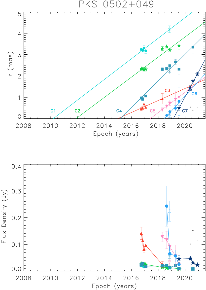
Figure 2: Top panels: angular separation from the core of the jet components in TXS 0506+056 (left panel) and PKS 0502+049 (right panel) as a function of time. Solid symbols correspond to 15 GHz observations data derived from multi-epoch observations. Coloured open symbols and black circles represent, respectively, the identified jet components in PKS 0502+049 at 8 GHz and those components identified in TXS 0506+056 by Ros et al. (2020) at 43 GHz. Unidentified components are shown by black points The straight lines represent linear regressions fitting for the individual jet components. Bottom panels: flux density evolution of the jet components as a function of time for both sources.

3 Results

3.1 Kinematics of the jets components

The kinematic analysis at parsec scales requires the identification of jet components across consecutive epochs in our data set. Based on Caproni et al. (2014), we assumed a kinematic scenario for the parsec-scale jet whose individual components recede ballistically or quasi-ballistically from the stationary core (constant proper motions along straight trajectories on the plane of sky). Thus, we were able to trace their motions studying the temporal evolution of flux densities and position angles, as well as their distances relative to the (stationary) core.

Thereby, the top panels in Figure 2 show the time evolution of the core-component distance for each of the jet components identified in TXS 0506+056 and PKS 0502+049. The solid lines and the corresponding slopes represent their apparent proper motion ($\mu$) obtained by linear regression of the equation

$$r(t)=\mu\left(t-t_{0}\right)\;,$$ (2)

where $r$ is the core-component distance at the instant $t$, and $t_{0}$ is the ejection epoch of the jet component ($r(t_{0})=0$).

In the top left panel of Figure 2, the black circles represent the jet features identified in TXS 0506+056 at 43 GHz by Ros et al. (2020). It is interesting to note that all of these 43-GHz features can be associated with the jet components C7, C8, C9 and C10 identified in the present work.

Based on the broadly accepted shock-in-jet model (e.g., Konigl, 1981; Marscher & Gear, 1985; Hughes et al., 1985; Valtaoja et al., 1992; Türler et al., 2000), jet components represent shock waves propagating downward in a relativistic jet and go through three distinct stages: an initial stage dominated by inverse Compton cooling, a synchrotron-dominated loss stage, and a final phase where the losses are adiabatic. We can see from bottom panels in Figure 2 the time evolution of flux density of individual components identified in both blazars.

We list the kinematic parameters of each of these jet components for TXS 0506+056 and PKS 0502+049 in Table 1. The parameter $\beta_{\mathrm{app}}$ correspond to the apparent speed in units of $c$, while $\bar{\eta}$ represents the mean position angle of a jet component among $N_{\mathrm{epoch}}$ epochs used in the fit. Uncertainties for $t_{0}$ and $\mu$ were calculated from the linear fit, taking into account the errors on the individual positions of the jet components, while standard deviation of $\eta$ was used as an error estimator for $\bar{\eta}$. The numbers displayed in the last column give the probability $p$ of the chi-squared value to be less than or equal to the value obtained from the linear regressions presented in Figure 2.

Table 1: Kinematic parameters of the CE model-fitting jet components of TXS 0506+056 and PKS 0502+049 identified in this work.

Jet component	$t_{0}$	$\mu$	$\beta_{\mathrm{app}}$	$\bar{\eta}$	$N_{\mathrm{epoch}}$ a	$p^{\mathrm{b}}$
	(yr)	(mas yr-1)		(deg)
TXS 0506+056
C1	2007.99 $\pm$ 0.08	1.22 $\pm$ 0.12	25.5 $\pm$ 2.6	-182.5 $\pm$ 0.1	5	0.028
C2	2008.86 $\pm$ 0.11	0.85 $\pm$ 0.08	17.7 $\pm$ 1.7	-177.3 $\pm$ 0.5	6	0.066
C3	2009.96 $\pm$ 0.14	0.69 $\pm$ 0.07	14.4 $\pm$ 1.5	-173.3 $\pm$ 0.4	6	0.006
C4	2011.41 $\pm$ 0.13	0.62 $\pm$ 0.05	12.9 $\pm$ 1.0	-179.0 $\pm$ 0.1	8	0.472
C5	2013.20 $\pm$ 0.3	0.45 $\pm$ 0.15	9.5 $\pm$ 3.2	-168.1 $\pm$ 0.3	4	0.235
C6	2015.60 $\pm$ 0.07	1.28 $\pm$ 0.11	26.7 $\pm$ 2.2	-177.8 $\pm$ 0.2	6	0.492
C7	2016.58 $\pm$ 0.08	1.31 $\pm$ 0.14	27.2 $\pm$ 2.9	-175.0 $\pm$ 0.9	5	0.069
C8	2017.09 $\pm$ 0.09	1.06 $\pm$ 0.09	22.2 $\pm$ 2.0	-180.7 $\pm$ 0.3	6	0.789
C9	2017.72 $\pm$ 0.13	0.82 $\pm$ 0.16	17.0 $\pm$ 3.3	-174.1 $\pm$ 0.2	5	0.220
C10	2017.9 $\pm$ 0.4	0.4 $\pm$ 0.5	8 $\pm$ 11	-179.9 $\pm$ 0.2	2	1.000
C11	2019.66 $\pm$ 0.04	2.9 $\pm$ 0.8	60 $\pm$ 16	-176.4 $\pm$ 0.5	4	0.034
C12	2020.01 $\pm$ 0.03	3.2 $\pm$ 0.7	66 $\pm$ 14	-181.2 $\pm$ 1.3	5	0.590
PKS 0502+049
C1	2010.2 $\pm$ 0.5	0.48 $\pm$ 0.13	24.4 $\pm$ 6.6	-132.7 $\pm$ 0.6	5	0.100
C2	2011.9 $\pm$ 0.3	0.47 $\pm$ 0.08	23.9 $\pm$ 4.0	-130.0 $\pm$ 0.7	8	0.235
C3	2015.0 $\pm$ 0.4	0.28 $\pm$ 0.18	14.3 $\pm$ 9.1	-130.8 $\pm$ 5.9	5	0.072
C4	2015.17 $\pm$ 0.12	0.62 $\pm$ 0.06	31.6 $\pm$ 3.1	-129.0 $\pm$ 2.1	10	0.536
C5	2017.4 $\pm$ 0.2	0.5 $\pm$ 0.2	24 $\pm$ 12	-130 $\pm$ 9	6	<0.001
C6	2018.47 $\pm$ 0.17	0.7 $\pm$ 0.3	35 $\pm$ 16	-120 $\pm$ 24	4	0.058
C7	2019.13 $\pm$ 0.19	1.2 $\pm$ 0.2	59 $\pm$ 12	-127.3 $\pm$ 0.6	4	0.057

^a Number of epochs for which a given jet component was detected by our CE model fitting.

^b Probability that a chi-squared value is less than or equal to the value obtained in our linear regressions.

In the case of TXS 0506+056, the linear fit for the jet components C1, C2, C3, C7 and C11 exhibited the highest confidence levels among all the identified jet components ($p\leq 0.1$), while C10 has a questionable fitting if we adopt the usual criterion $p\leq 0.9$ (or similarly $q=1-p\geq 0.1$ for normal-distributed and well-estimated uncertainties; e.g., Press et al. 1992; Wasserman 2010) as a discriminator of the reliability of a fit. It was already expected since C10 was only detected in two epochs. In addition, correlation coefficient $r_{\mathrm{corr}}$ (e.g., Cohen 1988; Press et al. 1992; Heumann & Schomaker 2017; Gajendran et al. 2021) of these linear regressions is always larger than about 0.94, which can be considered as an indicative of reasonable fits. Even though these statistical tests argue in favour of the significance of the majority of those linear fits, the ad-hoc ballistic-motion assumption might have introduced some bias in such analyses in the sense that it was incorporated in the process of the kinematic identification of the individual jet components. Thus, both statistical tests used to quantify the goodness of the fits do not exclude permanently more complex kinematic scenarios for the parsec-scale jet of TXS 0506+056.

The core-component distance plot in Figure 2 shows a clear superposition between proper motion extrapolation of C5 (orange line) and the distance of C6 from the core between 2016.5 and 2017.5. The detection of C6 in 2016.1 independent of the number of Gaussian components assumed in our CE optimisations, as well as the difference of about 10 degrees between the mean position angles of C5 and C6 suggests the latter is real. In addition, the peak-like behaviour seen in the light curve of C6 (Figure 2) could be indicating a possible superposition between jet components C5 and C6 between 2016.5 and 2017.5, even though our CE optimisations were not able to detected (no splitting of C6 is found after increasing the number of components in our CE model fittings in this interval).

Good statistical reliability was found for five out of seven jet components identified in PKS 0502+049 ($p\la 0.1$ and $r_{\mathrm{corr}}\ga 0.92$). It is important to note that the lack of VLBI monitoring of PKS 0502+049 between 2017 and 2018 casts some doubts on the kinematic identifications of the jet components C1 and C2 shown in Figure 2. Even though the present data cannot rule out a scenario where C1 and C2 are standing or slowly moving jet features (as observed in many other blazars), their inferred emergence epochs coincide with a flaring state of the source at gamma-ray energies as seen in Figure 3, providing extra support for our C1 and C2 identifications. Whether or not C1 and C2 are quasi-stationary components does not exert any influence on the results presented in the next sections of this work. The identification of the jet component C3 might also be impacted by the same one-year data gap mentioned previously. However, the occurrence of strong gamma-ray flares during the emergence of C3 argues in favour of its possible existence.

Since time-correlation between the radio and gamma-ray activity has been found in other AGNs (e.g., Max-Moerbeck et al., 2014; Richards et al., 2014), as well as the relationship between ejection of new jet components and occurrence of flares in gamma-rays (e.g., Otterbein et al., 1998; Jorstad et al., 2001; Agudo et al., 2011; Cutini et al., 2014; Lisakov et al., 2017), we looked for similar correlations in the case of TXS 0506+056 and PKS 0502+049. We plot in Figure 3 the public data from the Fermi-LAT (see details in subsection 2.2), as well as the time behaviour of the parsec-scale core and total flux densities (the sum of the contributions from core and individual jet components). Vertical orange bars in this figure represent the 1$\sigma$-uncertainty range for the ejection epochs of the jet components. Except for component C1 in TXS 0506+056, for which no gamma-ray data is available at its ejection epoch, the remaining jet components have emergence epochs that coincide with enhanced activity seen in the Fermi-LAT gamma-ray light curve.

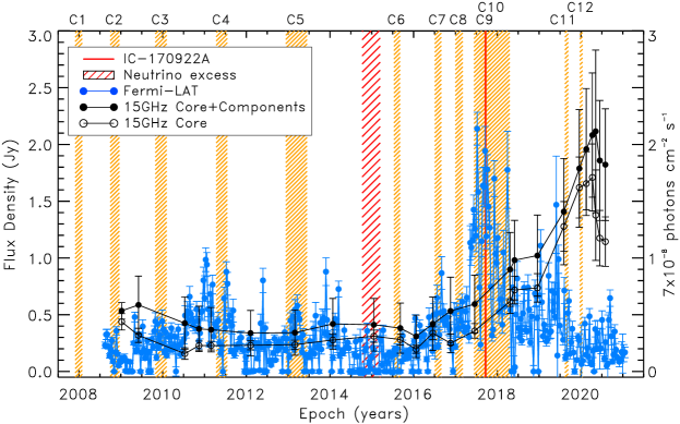
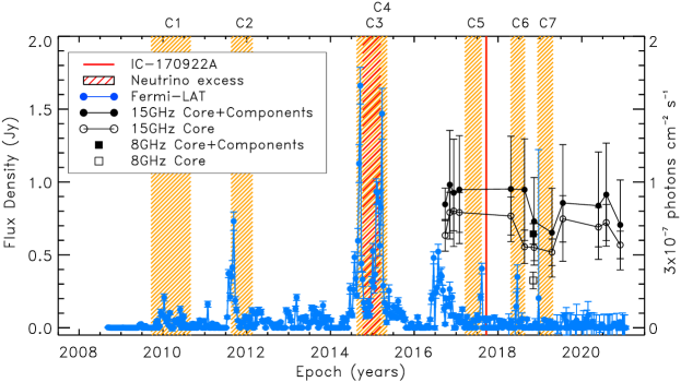
Figure 3: Flux density behaviour of TXS 0506+056 (top panel) and PKS 0502+049 (bottom panel). Solid and open black circles display the total (core plus jet components) and core flux densities at 15 GHz, respectively. Solid and open black square refer, respectively, to the total and core flux densities for the single 8-GHz observational epoch of PKS 0502+049. Fermi gamma-ray light curve is shown by blue circles. Vertical orange bars highlight the 1$\sigma$ uncertainty range for the ejection epochs of the jet components.

The radio flux density variability of the core plus jet components seen in Figure 3 is very similar to that obtained by Kun et al. (2019) for TXS 0506+056; these authors reported an increase of radio emission after the neutrino excess. Interestingly, in the period following the HE neutrino event IC-170922A, the observed radio flux roughly increased a factor of 4, being accompanied by the appearance of two new superluminal components (C11, C12). Our kinematic-based identification reveals that no component was ejected in TXS 0506+056 during the six-month period in 2014-2015 (see Figure 3), corroborating the temporarily quiescent state of this source in GeV emission.

Perhaps, one of the most important results in this work is the identification of the jet component C9, in TXS 0506+056, and C3 and C4, in PKS 0502+049. As already mentioned, PKS 0502+049 was in a state of enhanced gamma-ray emission just before and after the period of the neutrino excess. The jet component C3, whose apparent speed is $\beta_{\mathrm{app}}=14.3c$, has an estimated ejection time of $2014.99\pm 0.36$, coinciding with the 2014 gamma-ray flare and the neutrino excess. PKS 0502+049 also ejected a very bright moving feature, C4, in $2015.17\pm 0.12$, with an apparent speed of $31.6c$ in temporal coincidence with 2015 gamma-ray flare at $1\sigma$-level. The aforementioned events and their correlations can be seen in the bottom panel of Figure 3.

The direction of the reported event IceCube-170922A was consistent with the location of TXS 0506+056, which was observed in enhanced gamma-ray activity by Fermi-LAT. Corroborating the association of HE neutrino with TXS 0506+056, the jet component C9 identified in this work has an ejection epoch that coincides, within the uncertainties, with the event IC-170922A and the $\gamma$-ray flare that occurred on 22 September, 2017.

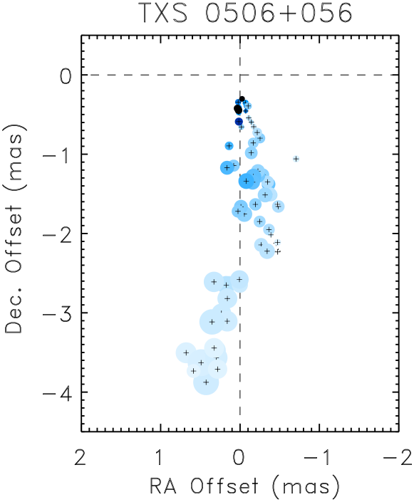
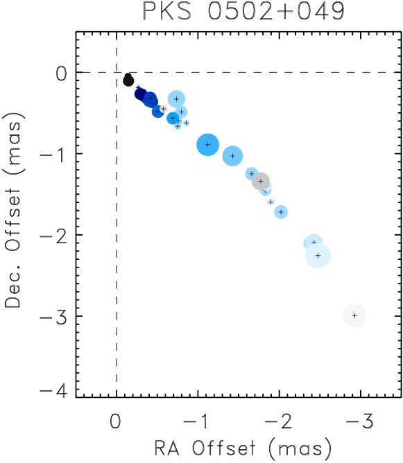
Figure 4: The distribution of right ascension and declination offsets of the jet components in TXS 0506+056 (left panel) and PKS 0502+049 (right panel) at 8 GHz (grey circle) and 15 GHz (blue circle). The size of the symbols is proportional to the semi-major axis of the jet components, while the shades of the colors are proportional to the jet component’s brightness, namely darker colors represent brighter components.

The spatial distribution of right ascension and declination offsets of the jet components relative to the position of the VLBI core is shown in Figure 4. TXS 0506+056 has a jet-component distribution that extends approximately in a direction close to North-South. A more pronounced and systematic jet bending occurs at a core distance of $\sim 2.5$ mas, which was interpreted in the framework of two distinct scenarios: a helical jet structure (Kun et al., 2019) and two relativistic jets in collision (Britzen et al., 2019). Ros et al. (2020) analysed two 43-GHz images of the radio jet of TXS 0506+056 and concluded that they do not show any clear isolated knots of locally enhanced brightness temperature that could be associated with a secondary jet inlet region located $\sim 1.2$ mas apart from the (primary) core, as suggested by Britzen et al. (2019). Similarly to Ros et al. (2020), we have not identified any bright and persistent feature at the same region that could be attributed to the origin of a secondary jet in TXS 0506+056.

The wider jet-component distribution along the right ascension direction for a given declination offset in TXS 0506+056 suggests that jet orientation could have changed during the VLBI monitoring period analysed in this work. Moreover, the variations in the individual apparent speeds and position angles of the jet components shown, e.g., in Table 1 seems to corroborate such possibility. Jet precession is one of the physical mechanisms that could drive those temporal changes. Indeed, Britzen et al. (2019) constructed a precession model for TXS 0506+056 based on the equations discussed in earlier papers in the context of other blazars (e.g., Abraham, 2000; Caproni & Abraham, 2004a; Britzen et al., 2018), establishing a precession model for TXS 0506+056 where a mildly relativistic jet ($\gamma\sim 2.6$) crosses the line of sight every $\sim 5$ years (precession period of about 10 years).

Regarding PKS 0502+049, the right panel in Figure 4 shows a narrower jet-component distribution along the right ascension direction for a fixed declination offset in comparison with that seen in TXS 0506+056. Despite the geometrical interpretation (changes in the jet direction) mentioned previously, the wider scatter observed for the components of TXS 0506+056 on the plane of the sky could also be a consequence of the different observational characteristics of these two blazars: as TXS 0506+056 and PKS 0502+049 are located at distinct redshifts, their angular scales are not the same (roughly a factor of two larger in the case of TXS 0506+056), as well as the interval between first and last epoch of the maps used in this work (the observations of TXS 0506+056 span a time range measured at its rest frame that is about a factor of 5 larger than the corresponding interval for PKS 0502+049). In addition, the initial NE-SW orientation of the parsec-scale jet of PKS 0502+049 suffers a clear and systematic bending towards south direction after a core distance of $\sim 2.2$ mas.

3.2 General constraints for the parsec-scale jets of TXS 0506+056 and PKS 0502+049

All jet components here identified exhibit superluminal speeds ranging from $9.5c$ to $66.5c$ and from $14.3c$ to $59.1c$ for TXS 0506+056 and PKS 0502+049, respectively. The apparent superluminal velocities $\beta_{\mathrm{app}}$ depend on the Lorentz factor $\gamma$ and on the viewing angle $\theta$ through the relation:

$$\beta_{\mathrm{app}}=\frac{\sin\theta}{\gamma\left(\gamma^{2}-1\right)^{-1/2}-\cos\theta}\;.$$ (3)

where

$$\gamma={(1-\beta^{2})^{-1/2}}$$ (4)

and $\beta$ is the bulk velocity of the jet.

The apparent velocities has a maximum value ${\beta_{\mathrm{app}}^{\mathrm{max}}}$ when $\cos\theta=\beta$; the minimum value of the relativistic Lorentz factor that satisfies this relation is:

$$\gamma_{\mathrm{min}}=\sqrt{1+(\beta_{\mathrm{app}}^{\mathrm{max}})^{2}}\;,$$ (5)

Our fastest (and reliable) identified jet components, C11 in the case of TXS 0506+056 and C7 in PKS 0502+049, imply $\gamma_{\mathrm{min}}=66\pm 14$ and $\gamma_{\mathrm{min}}=59\pm 11$, respectively. Note that the Lorentz factor estimated for TXS 0506+056 differs from those found in Kun et al. (2019) and Li et al. (2020) ($\gamma\sim 5$), since the apparent speeds found in this work are substantially higher than those inferred in former studies. Potential reasons for such discrepancy might be related to the identification scheme for jet components adopted in this work (see subsection 3.1), as well as the usage of an image-based decomposition of the interferometric maps through the CE technique instead of visibility model-fits done in previous works. A denser monitoring of the parsec-scale jet of TXS 0506+056 in future (similar to that seen in Figure 2 after mid 2019, as well as perfomed for other sources; e.g., Blasi et al. 2013; Jorstad et al. 2017) is crucial for confirming the proposed jet-component identification in this work.

On the other hand, the maximum value of the angle between the jet orientation and the line of sight can be calculated from

$$\theta_{\mathrm{max}}\approx\arccos{\left[\frac{(\beta_{\mathrm{app}}^{\mathrm{min}})^{2}-1}{(\beta_{\mathrm{app}}^{\mathrm{min}})^{2}+1}\right]}\;,$$ (6)

where $\beta_{\mathrm{app}}^{\mathrm{min}}$ is the lowest apparent speed among detected jet components.

We found maximum viewing angles of $12\degr\pm 4\degr$ and $8\degr\pm 5\degr$ for TXS 0506+056 and PKS 0502+049, respectively. In the case of TXS 0506+056, Li et al. (2020) obtained a jet viewing angle $\theta_{\mathrm{max}}=20\degr\pm 2\degr$, whereas Kun et al. (2019) found $\theta_{\mathrm{max}}=8\aas@@fstack{\circ}2$ using the average Doppler factor of the core.

Another relevant parameter related to jet kinematics is the Doppler boosting factor, $\delta$, defined as

$$\delta=\left[\gamma-\left(\gamma^{2}-1\right)^{1/2}\cos\theta\right]^{-1}\;.$$ (7)

Thus, estimates for $\delta$ associated with the robust jet components can be obtained from the previous knowledge of their jet viewing angles and Lorentz factors. Imposing $\gamma=\gamma_{\mathrm{min}}$ and using the values of $\beta_{\mathrm{app}}$ listed in Table 1, values of $\theta$ for each jet component can be determined from Equation 3.

Except for $\beta_{\mathrm{app}}=\beta_{\mathrm{app}}^{\mathrm{max}}=\sqrt{\gamma_{\mathrm{min}}^{2}-1}$, this procedure leads to two independent solutions for $\theta$, which translates consequently to two possible values for $\delta$ (see Equation 7). Considering all jet components found in this work, we derived possible ranges for $\delta$ in both sources, resulting to $0.5\la\delta\la 132$ for TXS 0506+056 and $1.8\la\delta\la 116$ for PKS 0502+049. Note that values of $\gamma$ higher than $\gamma_{\mathrm{min}}$ would broaden those ranges since the upper (lower) limit for $\delta$ would be shifted upwards (downwards) in relation to those calculated above.

3.3 Brightness temperature of the core region

The brightness temperature of the core region in the rest frame of the source, $T_{\mathrm{B,rest}}$, is defined as

$$T_{\mathrm{B,rest}}=(1+z)\,\frac{2\,\ln{2}}{\pi k}\frac{c^{2}}{\nu^{2}}\frac{F}{a_{\mathrm{FWHM}}\,b_{\mathrm{FWHM}}}\;,$$ (8)

where $z$ is the redshift of the host galaxy, $k$ is the Boltzmann constant, and $a_{\mathrm{FWHM}}$ and $b_{\mathrm{FWHM}}$ are, respectively, the FWHM of the elliptical Gaussian components along the major and the minor axes. In the case of an unresolved emitting region, the term $a_{\mathrm{FWHM}}\,b_{\mathrm{FWHM}}$ must be replaced by $d_{\mathrm{min}}^{2}$, which can be written as (Lobanov, 2005)

$$d_{\mathrm{min}}=\frac{2^{2-\varpi/2}}{\pi}\left[\pi\ln{2}\;\left(\Theta^{\mathrm{FWHM}}_{\mathrm{beam}}\right)^{2}\sqrt{1-\epsilon^{2}_{\mathrm{beam}}}\,\ln{\left(\frac{\mathrm{SNR}}{\mathrm{SNR}-1}\right)}\right]^{1/2}\;,$$ (9)

where SNR (= $I_{\mathrm{max}}$/RMS) is the signal-to-noise ratio and $\varpi$ is an index describing the weighting method used to generate the radio maps ($\varpi=0$ for uniform weighting and $\varpi=2$ for natural weighting; Lobanov 2005).

We listed in LABEL:table:Parameters_PKS_8GHz_table the values of $T_{\mathrm{B,rest}}$ for the core, calculated from Equation 8. It ranges from $0.6\leq T_{\mathrm{B,rest}}(10^{11}\,$K$)\leq 8.5$ for TXS 0506+056 and $2.8\leq T_{\mathrm{B,rest}}(10^{11}\,$K$)\leq 39.8$ for PKS 0502+049.

In the upper left panel of Figure 5, we show the time behaviour of $T_{\mathrm{B,rest}}$, as well as $\beta_{\mathrm{app}}$ as a function of $t_{0}$ for TXS 0506+056. Since the epochs of the VLBI observations do not coincide with the ejection epochs of the superluminal components, the brightness temperature values are interpolations. A clear increase of $T_{\mathrm{B,rest}}$ by a factor of 3 is seen after the year 2016, which also coincides with the IceCube-170922A event. A more complicated behaviour is noted in the case of $\beta_{\mathrm{app}}$, which presents non-monotonic variations during the whole period of the interferometric monitoring. We do not discuss the behaviour of PKS 0502+049 because of the limited time coverage of the VLBI observations.

The measured brightness temperature is related to the intrinsic brightness temperature of the source at its rest frame $T_{\mathrm{B,int}}$ by the relation (e.g., Readhead, 1994; Kovalev et al., 2005; Homan et al., 2006):

$$T_{\mathrm{B,rest}}=\delta\,T_{\mathrm{B,int}}\;,$$ (10)

Readhead (1994) studied the distribution of intrinsic brightness temperatures of sample of blazars and concluded that they are concentrated around the equipartition value of $\sim 5\times 10^{10}$ K, and proposed the use of Equation 10 as a tool to calculate the Doppler factor. In the next subsection we apply this technique to calculate the variation of the physical parameters of the superluminal components of TXS 0506+056.

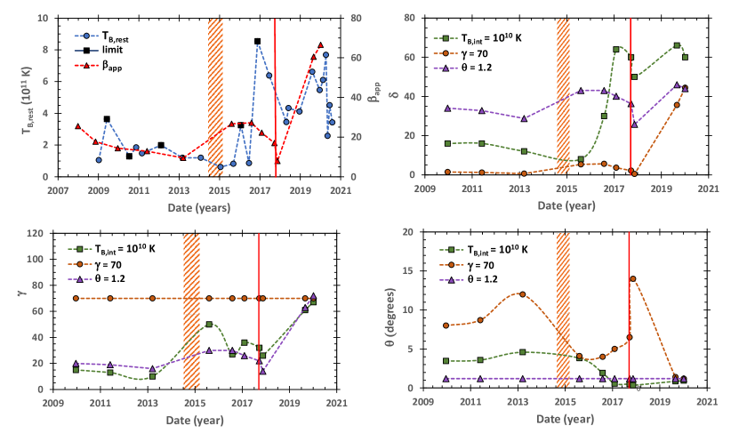
Figure 5: Upper left panel: The blue circles show the core’s brightness temperature at rest frame of TXS 0506+056 as a function of time. When core is unresolved, a lower limit for the brightness temperature is provided and marked by black squares. The apparent speed of each jet component of TXS 0506+056 in terms of their respective ejection epochs are displayed by red triangles. Upper right panel: Doppler boosting factors derived at the ejections epochs of the jet components assuming a constant value for $T_{\mathrm{B,int}}(=10^{10})$ K (green squares), a constant value for $\gamma(=70)$ (red circles), and a constant value for $\theta(=1\aas@@fstack{\circ}2)$ (purple triangles). Lower left panel: The same of the previous panel but showing the behaviour of the jet bulk Lorentz factor. Lower right panel: The same of the previous panel but showing the behaviour of the jet viewing angle. The epochs of the neutrino excess and the IceCube-170922A event are marked respectively by the hatched red rectangle and the vertical red line in all the panels.

Figure 6: The values of Lorentz factor (red circles), Doppler factor (green squares), and jet viewing angle (purple triangles) at the ejection epochs of the jet components in TXS 0506+056 considering $T_{\mathrm{B,int}}=1\times 10^{10}$ K (left panel) and $T_{\mathrm{B,int}}=2\times 10^{10}$ K (right panel). The epochs of the neutrino excess and the IceCube-170922A event are marked respectively by the hatched red rectangle and the vertical red line in both panels.

3.4 Temporal changes of the jet parameters

In blazars, the Doppler factor of the jet is one of the most important input parameters for the models that aim to reproduce the observed neutrino observations and their relation to different electromagnetic frequencies; its value depends on the Lorentz factor and on the jet direction relative to the line of sight. The same dependence affects the value of the apparent superluminal velocities. The jet direction is assumed to be perpendicular to the accretion disk (e.g., Jones et al. 2000) and frequently the differences between the apparent superluminal velocities of the jet components are attributed to differences in the viewing angles of the jet at the epoch at which the components were ejected (e.g., Homan et al. 2003). For many objects, the variations of the jet direction were attributed to precession; the Lorentz factor was assumed to be constant along the precessing period and its value was determined fitting the models (viewing and position angles on the plane of the sky) to the observations; variations of the Doppler factor with time were calculated from the precessing model and the constant value of the Lorentz factor (e.g., Gower et al. 1982; Romero et al. 2000; Caproni & Abraham 2004b; Kudryavtseva et al. 2011; Roland et al. 2013; Caproni et al. 2017; Britzen et al. 2018).

In the case of TXS 0506+056, it is not clear that the variations of $\beta_{\mathrm{app}}$ with time are due to precession. In fact, even if the aperture of the precession cone is small, as implied from the minimum and maximum viewing angles, their small absolute values require variations of the projected angle on the plane of the sky much larger than what is observed. However, we can still calculate the Doppler factor from Equation 10, assuming a constant intrinsic brightness temperature for the blazar. We show the results of this calculation in the top right panel of Figure 5 (green squares), which shows the variation of the Doppler factor with time assuming the constant value $T_{\mathrm{B,int}}=10^{10}$ K. Once the Doppler factor is known, the Lorentz factor and the viewing angle can be calculated from Equations 7 and 3, respectively. Their time dependence is shown as green squares at the bottom left and right panels of Figure 5, respectively. The same results are shown in the left panel of Figure 6, where we can also see in the right panel, the variation with time of the Doppler and Lorentz factors, and the jet viewing angle, obtained using $2\times 10^{10}$ K for the constant intrinsic brightness temperature. The value of $10^{10}$ K is the lowest compatible with the observations, since it renders a maximum value of the Lorentz factor $\gamma=67$, close to what is necessary to obtain the observed maximum apparent velocity. As expected, the increase of $T_{\mathrm{B,int}}$ produces a decrease in $\delta$ (see Equation 10) for all epochs, leading to a systematic increase of $\theta$. The solution with the highest brightness temperature also predicts too extreme values for $\gamma$ ($\sim 90$) in two epochs, 2015.6 and 2020.0, arguing in favour of constant-$T_{\mathrm{B,int}}$ models with intrinsic brightness temperatures lower than $2\times 10^{10}$ K.

The Doppler and Lorentz factors, as well as the viewing angle of the jet can also be calculated from Equations 3, 4 and 7, assuming a constant value for one of these parameters. This has been done and it is shown in the top right and bottom left and right panels of Figure 5 as red circles for constant $\gamma=70$, and purple triangles for constant $\theta=1.2\degr$. Again, the constant parameters $\gamma$ and $\delta$ have values close to the minimum compatible with the observed maximum apparent velocity.

Analysing the results for the Doppler factor presented in the top right panel of Figure 5, we can see that when the Lorentz factor is maintained constant, the value of $\delta$ remains low $(<10)$, except for the two last epochs in which it increases by a factor of 4; when it is the viewing angle that remains constant, $\delta$ has a large value during all the observing period, but when it is the intrinsic brightness temperature that remains constant, $\delta$ has a sharp increase between 2016 and 2017, which can explain, by boosting, the high emission in $\gamma$ rays that was observed starting at this epoch and which coincides with the neutrino detection.

Regarding the Lorentz factor, when the intrinsic brightness temperature is maintained constant, we can see an increase in $\gamma$ by a factor of three between 2013 and 2016, which maybe could be related to the neutrinos detected between 2014 and 2015. Both $T_{\mathrm{B,int}}$ and $\theta$ constant require a large increase in the Lorentz factor at latter epochs to account for the high value of the superluminal velocities.

Finally, when we compare the behaviour of the viewing angle when $T_{\mathrm{B,int}}$ or $\gamma$ are constant, we can see that when $T_{\mathrm{B,int}}$ is constant, $\theta$ remains almost constant at $4\degr$ until 2016 and then it drops to about $1\degr$, while when $\gamma$ is maintained constant, $\theta$ reaches much larger values and have irregular variability.

It is important to note that the whole analyses above assumed that two out of the three free parameters used to describe $T_{\mathrm{B,int}}$ and $\beta_{\mathrm{app}}$ at the ejection epochs of the jet components in TXS 0506+056 can change in time, which does not exclude the possibilities of just one or even all the three parameters could be time variable.

4 Discussion

As mentioned previously, our results regarding the kinematics of the parsec-scale jets of TXS 0506+056 and PKS 0502+049 show that ejections of new components coincide (at 1$\sigma$-level) with the appearance of flares in their respective gamma-ray light curves. Moreover, the formation epochs of the jet components C9 and C10 in TXS 0506+056 are compatible with the occurrence of the IceCube-170922A event, suggesting a possible connection between the radio core activity and the production of the detected 290-TeV neutrino. A systematic and strong increase of the flux density of the parsec-scale core of TXS 0506+056 seen after 2017 (see Figure 3) also argues in favour of this possibility.

Indeed, AGN core regions as sites of production of neutrinos have been recently proposed in the literature. Plavin et al. (2020) analysed statistically the origin of IceCube neutrinos with energies higher than $\sim$200 TeV using VLBI data and single-dish radio observations of 18 AGNs. They found that these AGNs usually have more intense parsec-scale cores in comparison with other radio-loud sources, with their sites of high-energy neutrinos residing at distances lower or of the order of some parsecs from the SMBH. Plavin et al. (2021) extended those analyses, including all neutrinos detected by IceCube collaboration between 2008 and 2015, as well as relaxing the lower limit of $\sim$200 TeV adopted previously. They found that the association between neutrino production and blazar activity also exists for lower neutrino energies as well.

Neronov & Semikoz (2020) proposed a scenario to explain the correlation between radio emission and high-energy neutrinos associated with AGNs reported by Plavin et al. (2020). Their model considers that both synchrotron emitting electrons and neutrinos originate from decays of charged pions produced in proton-proton interactions in parsec-scale relativistic jets. The exact location of the site where neutrinos are produced depends on the density profile of the interstellar medium of these galaxies, not exceeding parsec-scale distances from the SMBH. Previously, Keivani et al. (2018) considered single-zone theoretical models (neutrinos and gamma-rays produced at the same site) to study the relationship between the IceCube-170922A event and the contemporaneous electromagnetic emission from near-infrared to gamma-ray energies. They found that a hybrid leptonic scenario (gamma-rays produced by inverse-Compton scatterings and high-energy neutrinos via a radiatively subdominant hadronic component) can fairly describe the observed electromagnetic and neutrino fluxes. Hovatta et al. (2020) found that a fraction of neutrino events are not associated with strong radio flaring blazars after correlating the radio data from the Owens Valley Radio Observatory and Metsähovi Radio Observatory blazar monitoring programs with the IceCube neutrino events. However, a random coincidence is strongly disfavour when a large amplitude radio flares in a blazar is observed together with a concomitant and spatially coincident neutrino event according to these authors.

Considering the results shown in Figure 5 and Figure 6, the bulk Lorentz factor of the parsec-scale jet of TXS 0506+056 ranges roughly between 10 and 70, which agrees with values invoked in some theoretical models used to interpret the IceCube-170922A event (e.g., Banik & Bhadra, 2019; Zhang et al., 2020). Regarding the Doppler boosting factor, those theoretical models have adopted values between $\sim 5$ and 30, in good agreement with the cases $\theta=1\aas@@fstack{\circ}2$ (Figure 5) and $T_{\mathrm{B,int}}=2\times 10^{10}$ K (Figure 6).

On the other hand, the neutrino excess detected by IceCube collaboration between September 2014 to March 2015 coincides with a relative quiescent phase seen in the gamma-ray light curve of TXS 0506+056 (e.g., Padovani et al., 2018; Garrappa et al., 2019), as well as the lack of any substantial parsec-scale core activity and/or emergence of any new jet component (see Figure 3, for instance). Indeed, neutrino production without a clear electromagnetic counterpart (an “orphan" neutrino flare; e.g., Xue et al. 2020) brought challenges to some theoretical (single-zone) models since an electromagnetic cascade that follows neutrino emission is expected in such situation (e.g., IceCube Collaboration et al., 2018; Rodrigues et al., 2019; Reimer et al., 2019; Xue et al., 2020).

Several theoretical models focusing on the 2014-2015 neutrino excess are available in the literature. For instance, Reimer et al. (2019) concluded that the neutrino excess was probably generated through hadronic interactions of relativistic protons with a stationary (in relation to the rest frame of the galaxy) soft X-ray photon field.These authors also found that the predicted GeV gamma-ray flux produced by inverse Compton during pair cascades is too low in comparison to the observed Fermi-LAT flux from TXS 0506+056, concluding that neutrinos and gamma-rays are probably generated by distinct physical processes. Similarly, Rodrigues et al. (2019) analysed the viability of leptohadronic models with three different geometries (one zone, compact-core, and additional external photon field) to explain simultaneously the spectral energy distribution of TXS 0506+056 and the IceCube neutrino spectrum, as well as the quantity of neutrinos ($13\pm 5$) produced in such event. Difficulties in fulfilling simultaneously the observation constraints from electromagnetic and neutrino spectra were found independently of the adopted model. Moreover, they concluded that obtaining more than two to five neutrino events during the period between September 2014 and March 2015 implies violating the multi-wavelength constraints. Similar difficulties in describing simultaneously electromagnetic data and neutrino emission produced at the same site have been faced by other recent works (e.g., Petropoulou et al., 2020). In contrast, Zhang et al. (2020) proposed a model that provides an explanation for the 2014–2015 neutrino excess without disrespecting the X-ray and gamma-ray observational constraints. In their model, protons and other heavier nuclei are accelerated in a compact region (blob) of blazar jets. Their interaction with radiation fields are able to generate not only high-energy photons, but also electron–positron pairs, neutrinos, and neutrons. Neutrinos and neutrons can freely escape from the blob whereas the high-energy photons may be trapped by local opacity effects.

One of the radio maps of TXS 0506+056 analysed in this work was obtained on 2015 January 18 (2015.049), roughly in the middle of the reported neutrino-excess time window (IceCube Collaboration, 2018). Our CE modelling of this image revealed the presence of a superluminal jet component, C5, at a core-component angular distance of $\sim 0.84$ mas, corresponding to a projected distance, $L_{\mathrm{proj}}$, of about 4.0 pc at the redshift of TXS 0506+056. The deprojected core-component distance, $L$ (calculated from $L=L_{\mathrm{proj}}/\sin\theta$), has a lower limit of about 19 pc considering a jet viewing angle of $\sim 12\degr$ (upper limit value derived from Equation 6), and an upper limit of about 191 pc considering the model with $\theta=1\aas@@fstack{\circ}2$ shown in Figure 5. The predicted Doppler factor during the neutrino excess ranges roughly from 5 to 40, depending of the case displayed in Figures 5 and 6. They agree with the adopted values in current neutrino models (e.g., Rodrigues et al., 2018; Reimer et al., 2019; Zhang et al., 2020). Even though the derived FWHM semi-major axis of C5 ($\sim 0.38$ mas or $\sim 1.8$ pc) is substantially larger than usual radii of the blobs adopted in neutrino-production models ($\la 0.03$ pc; e.g., Murase et al., 2018; Reimer et al., 2019; Zhang et al., 2020), we speculate that the parsec-scale jet component C5 in TXS 0506+056 might be the site where 2014-2015 neutrino excess was produced. Of course this possibility must be validated by appropriated neutrino-production models in future works.

An alternative to TXS 0506+056 as the unique driver of the 2014–2015 IceCube neutrino excess has also been proposed in the literature (e.g., Liang et al., 2018; He et al., 2018; Banik et al., 2020). In this scenario, the gamma-ray loud PKS 0502+049 (separated by $\sim 1\aas@@fstack{\circ}2$ from TXS 0506+056) could be responsible for a fraction of the muon-neutrino events detected between September 2014 and March 2015. The median angular resolution of the muon-neutrino events detected by IceCube is about $0\aas@@fstack{\circ}5$ at energies around $\sim 30$ TeV (e.g., IceCube Collaboration, 2018). However, the directional reconstruction uncertainty for each individual neutrino event ranges from $\sim 0\aas@@fstack{\circ}2$ to more than 2°(e.g., Liang et al., 2018), which does not exclude the possibility that PKS 0502+049 could have contributed to the observed neutrino excess. Indeed, Liang et al. (2018) calculated the individual uncertainties regarding the neutrino trajectories and found that 7 out of the 13 neutrino events are spatially consistent with the sky position of PKS 0502+049. This result agrees with Rodrigues et al. (2019) who found difficulties in producing more than five neutrino events in their models without violating the multi-wavelength constraints for TXS 0506+056 between the epochs 2014 and 2015. Interactions between the relativistic jet and dense clouds associated with the broad line region of PKS 0502+049 have been invoked as drivers of neutrinos related to 2014-2015 Icecube event (He et al., 2018), while Banik et al. (2020) proposed a proton blazar jet scenario (e.g., Mücke & Protheroe, 2001; Banik & Bhadra, 2019) where non relativistic protons would be targets for the production of high-energy gamma rays and neutrinos via proton-proton interactions (due to the presence of relativistic protons in the jet). Banik et al. (2020) showed that neutrino excess observed during 2014–2015 is incompatible with the premise that TXS 0506+056 would have been the unique source responsible for such neutrinos. Indeed, their results suggest that PKS 0502+049 may be (partially or totally) responsible for the 2014–2015 neutrino excess. The adopted values $\delta=40$ and $\theta=1\aas@@fstack{\circ}35$ by Banik et al. (2020) are compatible with the values of these quantities derived in this present work ($2\lesssim\delta\lesssim 116$, $\theta\lesssim 8\degr$), even though their adopted value for the Lorentz factor ($\gamma=30$) is almost a factor of two lower than $\gamma_{\mathrm{min}}$ derived in this work ($\gamma\ga 59$).

It is important to emphasise that the observed gamma-ray flaring state of PKS 0502+049 has motivated several studies (as previously reported above) regarding the viability of this quasar as the main driver of the IceCube neutrino excess. In this work we report for the first time a possible connection between 2014-2015 gamma-ray flares and the formation of new jet components in PKS 0502+049. We can note in Figure 3 that jet components C3 and C4 were ejected during the occurrence of gamma-ray flares, which could be the sites where electromagnetic/neutrino emissions take place in some neutrino production models. Unfortunately, there is no interferometric data of PKS 0502+049 publicly available during the ejection period of C3 and C4 that allow us to infer any simultaneous flaring activity of the core region.

5 Conclusions

In this work, we presented the first kinematic study of the parsec-scale jet of the FSRQ PKS 0502+049 based on 13 interferometric images at 8 and 15 GHz. We have also thoroughly investigated the kinematic properties of the parsec-scale jet of TXS 0506+056 at 15 GHz, using 24 VLBA observations spanning the years 2009–2020. Based on the assumption that the jet emission can be modelled by discrete components described mathematically by two-dimensional elliptical Gaussian functions, we applied our CE global optimisation technique to determine the structural parameters of these Gaussian components.

The parsec-scale jet of PKS 0502+049 is highly relativistic, exhibiting seven moving components with apparent speeds ranging from $14.3c$ and $59.1c$, and pointing close to the line of sight ($\theta\la$ 8°$\pm$ 5°). The maximum observed speed implies a minimum jet Lorentz factor of 59 $\pm$ 11 for this source.

In the case of TXS 0506+056, we have identified twelve components in the parsec-scale jet receding ballistically from the core with superluminal apparent speeds (from $9.5c$ to $66c$). Through the fastest jet component we inferred a lower limit of 66 for the jet bulk Lorentz factor, and from the lowest apparent speed we obtained a conservative upper limit of $12\degr$ for the jet viewing angle, in agreement with previous estimates found in the literature. A novel approach using simultaneously the brightness temperature of the core region and the apparent speeds of the jet components allowed us to infer some basic jet parameters for TXS 0506+056 at distinct epochs. These results are in full agreement with the limits of $\gamma$, $\theta$ and $\delta$ determined from jet kinematics only.

In addition, we analysed the Fermi-LAT data from 300 MeV to 300 GeV to generate gamma-ray light curves for TXS 0506+056 and PKS 0502+049. Our results showed that the occurrence of gamma-ray flares fall within $1\sigma$ uncertainties of the ejection epochs of new components in both blazars. Furthermore, the ejection of the jet components C9 and C10 in TXS 0506+056 were contemporaneous with the occurrence of the IceCube-170922A event. Thus, we essentially suggest that the neutrino production may be connected with the radio core activity.

During the neutrino excess detected by the IceCube in 2014-2015, the blazar TXS 0506+056 was found to be in a quiescent phase in gamma-rays. Neither parsec-scale core activity nor emergence of any new jet component were observed during this period. However, the presence of the jet component C5 at the arrival time window of such a neutrino excess might indicate it is a potential site of neutrinos. As already mentioned, this scenario must be validated by a proper neutrino-production model.

An alternative to TXS 0506+056 as the unique driver of such thirteen observed muon neutrinos has also been proposed in the literature (e.g., Liang et al., 2018; He et al., 2018; Banik et al., 2020). As the nearby gamma-ray flaring blazar PKS 0502+049 was in the state of enhanced emission at GeV energies during the reported neutrino excess time window, it could have contributed for this event too. Interestingly, we found that this gamma-ray enhancement was accompanied by ejections of two superluminal jet components (C3 and C4) in PKS 0502+049, suggesting that these components could be jet blobs, namely the emitting region in some models of neutrino production in AGN.

In summary, although our findings strongly corroborate the previous association between TXS 0506+056 and the IceCube-170922A event, they are still inconclusive regarding the 2014-2015 neutrino excess. We highlight that our results do not rule out the possibility of both sources, TXS 0506+056 and PKS 0502+049, had emitted these $13\pm 5$ signal events quoted by the IceCube Collaboration as well.

Data Availability

The data underlying this article were accessed from the MOJAVE webpage (http://www.physics.purdue.edu/MOJAVE/index.html), the Fermi data server (https://fermi.gsfc.nasa.gov/cgi-bin/ssc/LAT/LATDataQuery.cgi), and the Astrogeo Center (http://astrogeo.org/vlbi_images/). The data generated in this research will be shared on reasonable request to the corresponding author.

Appendix A VLBI data

We provide in this section the basic characteristics of the radio interferometric images of TXS 0506+056 and PKS 0502+049 analysed in this work, as well as the structural parameters of the elliptical Gaussian components found after CE optimisation of those images.

Table 2: Quantitative characteristics of the 24 radio images of the blazar TXS 0506+056 analysed in this work.

Epoch	Frequency	$\Theta^{\mathrm{FWHM}}_{\mathrm{beam}}$	$\epsilon$	$\theta$	RMS	$I_{\mathrm{max}}$
	(GHz)	(mas)		(deg)	(mJy beam-1)	(Jy beam-1)
2009-01-07	15	1.40	0.89	-3.87	0.15	0.42
2009-06-03	15	1.34	0.90	-6.86	0.18	0.44
2010-07-12	15	1.38	0.93	-8.48	0.18	0.27
2010-11-13	15	1.37	0.91	-9.12	0.15	0.25
2011-02-27	15	1.18	0.89	-0.76	0.21	0.23
2012-02-06	15	1.29	0.89	-5.41	0.14	0.24
2013-02-28	15	1.24	0.90	-3.80	0.16	0.24
2014-01-25	15	1.20	0.88	-5.47	0.07	0.31
2015-01-18	15	1.34	0.92	-4.78	0.08	0.30
2015-09-06	15	1.27	0.91	-6.21	0.08	0.27
2016-01-22	15	1.33	0.91	-9.78	0.07	0.21
2016-06-16	15	1.17	0.90	-2.43	0.07	0.32
2016-11-18	15	1.19	0.90	-4.74	0.07	0.40
2017-06-17	15	1.18	0.90	-5.86	0.09	0.45
2018-04-22	15	1.21	0.90	-5.64	0.09	0.71
2018-05-31	15	1.19	0.90	-3.25	0.09	0.80
2018-12-16	15	1.21	0.88	2.44	0.13	0.84
2019-08-04	15	1.23	0.91	-5.30	0.07	1.26
2019-12-17	15	1.33	0.89	-6.40	0.08	1.59
2020-02-16	15	1.39	0.89	-7.52	0.09	1.73
2020-04-09	15	1.78	0.90	22.82	0.09	1.85
2020-05-08	15	1.33	0.88	-2.64	0.09	1.83
2020-06-13	15	1.23	0.92	-2.60	0.10	1.49
2020-08-01	15	1.24	0.90	0.03	0.10	1.45

Table 3: Quantitative characteristics of the 13 radio images of the blazar PKS 0502+049 analysed in this work.

Epoch	Frequency	$\Theta^{\mathrm{FWHM}}_{\mathrm{beam}}$	$\epsilon$	$\theta$	RMS	$I_{\mathrm{max}}$
	(GHz)	(mas)		(deg)	(mJy beam-1)	(Jy beam-1)
2016-09-26	15	1.15	0.90	-5.47	0.09	0.66
2016-11-06	15	1.22	0.91	-7.59	0.09	0.79
2016-12-10	15	1.44	0.89	12.14	0.09	0.81
2017-01-28	15	1.33	0.91	-6.66	0.09	0.79
2018-04-22	15	1.19	0.90	-4.89	0.09	0.78
2018-08-19	15	1.05	0.89	-4.57	0.11	0.76
2018-11-03	8	2.00	0.90	-2.16	0.46	0.50
2018-11-11	15	1.06	0.87	0.54	0.11	0.59
2019-04-15	15	1.19	0.89	-2.55	0.11	0.53
2019-07-19	15	1.91	0.95	-17.95	0.09	0.76
2020-05-25	15	1.96	0.94	-18.84	0.09	0.70
2020-08-01	15	1.23	0.90	0.97	0.09	0.77
2020-01-12	15	1.24	0.89	-5.67	0.07	0.58

Table 4: CE model-fitting jet parameters for the 15-GHz maps of TXS 0506+056. Columns from left to right refer, respectively, to observation epoch, component label, flux density, component distance, position angle, FWHM major axis, axial ratio between minor and major axes, structural position angle and observed brightness temperature corrected to the rest frame of TXS 0506+056.

Epoch	IDa	$F$	$r^{\mathrm{b}}$	$\eta^{\mathrm{c}}$	$a_{\mathrm{FWHM}}$	Axial Ratio	$\mathrm{SPA}^{\mathrm{c,d}}$	$T_{\mathrm{B,rest}}$
		[Jy]	[mas]	[deg]	[mas]		[deg]	$10^{11}\,\mathrm{K}$
2009.019	Core	0.438 $\pm$ 0.072	0.01 $\pm$ 0.09	-66.6 $\pm$ 906.9	0.174 $\pm$ 0.005	1.000 $\pm$ 0.005	-138.10 $\pm$ 0.04	1.05 $\pm$ 0.18
	C1	0.064 $\pm$ 0.009	1.29 $\pm$ 0.10	-166.9 $\pm$ 4.2	0.996 $\pm$ 0.019	0.866 $\pm$ 0.005	-150.7 $\pm$ 4.5	-
	U	0.032 $\pm$ 0.004	2.63 $\pm$ 0.11	177.2 $\pm$ 2.3	1.281 $\pm$ 0.075	1.000 $\pm$ 0.002	-70.8 $\pm$ 3.3	-
2009.422	Core	0.319 $\pm$ 0.062	0.09 $\pm$ 0.09	10.7 $\pm$ 55.0	0.012 $\pm$ 0.080	0.899 $\pm$ 0.053	-7.2 $\pm$ 21.0	> 3.64
	C2	0.182 $\pm$ 0.044	0.31 $\pm$ 0.10	-166.7 $\pm$ 16.9	0.330 $\pm$ 0.014	1.000 $\pm$ 0.001	-162.0 $\pm$ 24.7	-
	C1	0.046 $\pm$ 0.008	1.64 $\pm$ 0.09	-163.5 $\pm$ 3.2	0.965 $\pm$ 0.038	0.866 $\pm$ 0.002	-17.8 $\pm$ 3.9	-
	U	0.041 $\pm$ 0.015	2.57 $\pm$ 0.10	175.7 $\pm$ 2.1	1.587 $\pm$ 0.042	0.870 $\pm$ 0.041	-64.8 $\pm$ 13.9	-
2010.529	Core	0.157 $\pm$ 0.050	0.14 $\pm$ 0.10	9.8 $\pm$ 35.3	0.014 $\pm$ 0.104	0.898 $\pm$ 0.066	-10.3 $\pm$ 22.3	> 1.29
	C3	0.149 $\pm$ 0.053	0.22 $\pm$ 0.11	-167.8 $\pm$ 22.8	0.247 $\pm$ 0.012	1.000 $\pm$ 0.001	-165.2 $\pm$ 24.1	-
	C2	0.089 $\pm$ 0.016	1.29 $\pm$ 0.08	-164.9 $\pm$ 3.7	1.095 $\pm$ 0.014	0.866 $\pm$ 0.006	-17.3 $\pm$ 2.2	-
	C1	0.029 $\pm$ 0.005	2.88 $\pm$ 0.09	174.9 $\pm$ 1.7	1.747 $\pm$ 0.035	0.867 $\pm$ 0.010	-37.8 $\pm$ 5.8	-
2010.869	Core	0.229 $\pm$ 0.040	0.04 $\pm$ 0.09	159.0 $\pm$ 142.8	0.101 $\pm$ 0.007	0.878 $\pm$ 0.035	-0.7 $\pm$ 3.3	1.85 $\pm$ 0.42
	C3	0.051 $\pm$ 0.009	0.64 $\pm$ 0.09	-168.3 $\pm$ 8.0	0.092 $\pm$ 0.038	0.984 $\pm$ 0.061	-56.0 $\pm$ 0.3	-
	C2	0.053 $\pm$ 0.007	1.90 $\pm$ 0.09	-172.9 $\pm$ 2.7	0.890 $\pm$ 0.026	0.913 $\pm$ 0.069	-54.8 $\pm$ 15.3	-
	U	0.023 $\pm$ 0.004	1.29 $\pm$ 0.09	-147.6 $\pm$ 4.0	0.351 $\pm$ 0.033	0.870 $\pm$ 0.046	-19.2 $\pm$ 20.3	-
	C1	0.020 $\pm$ 0.002	3.60 $\pm$ 0.10	168.9 $\pm$ 1.6	1.896 $\pm$ 0.094	0.998 $\pm$ 0.012	-122.1 $\pm$ 8.5	-
2011.159	Core	0.228 $\pm$ 0.038	0.01 $\pm$ 0.08	176.1 $\pm$ 544.6	0.101 $\pm$ 0.007	0.998 $\pm$ 0.014	-135.0 $\pm$ 2.1	> 1.48
	C3	0.068 $\pm$ 0.007	0.84 $\pm$ 0.08	-162.7 $\pm$ 5.4	0.725 $\pm$ 0.024	1.000 $\pm$ 0.000	-22.7 $\pm$ 28.1	-
	C2	0.045 $\pm$ 0.005	1.99 $\pm$ 0.09	-169.5 $\pm$ 2.3	0.862 $\pm$ 0.054	0.999 $\pm$ 0.019	-55.6 $\pm$ 6.1	-
	C1	0.027 $\pm$ 0.007	3.91 $\pm$ 0.11	173.7 $\pm$ 1.4	2.430 $\pm$ 0.122	0.868 $\pm$ 0.025	-163.2 $\pm$ 11.4	-
2012.101	Core	0.231 $\pm$ 0.040	0.01 $\pm$ 0.09	162.1 $\pm$ 421.0	0.038 $\pm$ 0.031	0.891 $\pm$ 0.164	-2.2 $\pm$ 17.0	> 1.99
	C4	0.029 $\pm$ 0.006	0.69 $\pm$ 0.10	-165.8 $\pm$ 7.4	0.240 $\pm$ 0.089	0.872 $\pm$ 0.044	-56.9 $\pm$ 6.4	-
	C3	0.049 $\pm$ 0.009	1.57 $\pm$ 0.12	-165.7 $\pm$ 3.3	0.949 $\pm$ 0.054	0.866 $\pm$ 0.002	-16.2 $\pm$ 3.7	-
	C2	0.030 $\pm$ 0.007	2.66 $\pm$ 0.19	179.9 $\pm$ 2.7	1.366 $\pm$ 0.061	0.867 $\pm$ 0.021	-35.9 $\pm$ 6.8	-
2013.162	Core	0.236 $\pm$ 0.040	0.02 $\pm$ 0.08	3.1 $\pm$ 199.2	0.120 $\pm$ 0.007	0.993 $\pm$ 0.051	-138.3 $\pm$ 2.8	1.20 $\pm$ 0.25
	C4	0.043 $\pm$ 0.005	0.74 $\pm$ 0.08	-163.0 $\pm$ 6.5	0.645 $\pm$ 0.024	1.000 $\pm$ 0.001	-28.9 $\pm$ 29.2	-
	C3	0.040 $\pm$ 0.009	2.14 $\pm$ 0.08	-172.9 $\pm$ 2.2	1.111 $\pm$ 0.024	0.867 $\pm$ 0.015	-60.6 $\pm$ 3.3	-
	C2	0.023 $\pm$ 0.007	3.64 $\pm$ 0.13	172.2 $\pm$ 1.7	2.553 $\pm$ 0.141	0.871 $\pm$ 0.054	-154.2 $\pm$ 15.3	-
2014.068	Core	0.278 $\pm$ 0.050	0.05 $\pm$ 0.08	13.2 $\pm$ 88.2	0.139 $\pm$ 0.021	0.867 $\pm$ 0.005	-150.3 $\pm$ 6.1	1.20 $\pm$ 0.43
	C5	0.074 $\pm$ 0.024	0.35 $\pm$ 0.12	-165.2 $\pm$ 15.3	0.391 $\pm$ 0.057	0.941 $\pm$ 0.228	-144.9 $\pm$ 28.7	-
	C4	0.039 $\pm$ 0.007	1.50 $\pm$ 0.10	-166.0 $\pm$ 3.2	1.154 $\pm$ 0.045	0.866 $\pm$ 0.005	-8.9 $\pm$ 4.3	-
	C3	0.029 $\pm$ 0.004	2.77 $\pm$ 0.11	176.4 $\pm$ 2.2	1.783 $\pm$ 0.080	1.000 $\pm$ 0.002	-80.2 $\pm$ 5.9	-
2015.049	Core	0.311 $\pm$ 0.054	0.04 $\pm$ 0.08	-2.8 $\pm$ 121.9	0.191 $\pm$ 0.007	0.999 $\pm$ 0.009	-139.1 $\pm$ 0.1	0.62 $\pm$ 0.12
	C5	0.062 $\pm$ 0.007	0.84 $\pm$ 0.10	-168.4 $\pm$ 5.9	0.761 $\pm$ 0.042	0.999 $\pm$ 0.011	-133.6 $\pm$ 1.9	-
	C4	0.040 $\pm$ 0.004	2.21 $\pm$ 0.10	-171.1 $\pm$ 2.3	1.298 $\pm$ 0.066	1.000 $\pm$ 0.004	-65.5 $\pm$ 3.5	-
2015.682	Core	0.281 $\pm$ 0.048	0.01 $\pm$ 0.08	170.4 $\pm$ 555.5	0.170 $\pm$ 0.002	0.866 $\pm$ 0.005	-177.2 $\pm$ 2.7	0.82 $\pm$ 0.14
	C5	0.066 $\pm$ 0.013	1.00 $\pm$ 0.08	-172.0 $\pm$ 4.7	0.989 $\pm$ 0.024	0.867 $\pm$ 0.016	-129.7 $\pm$ 3.0	-
	C4	0.035 $\pm$ 0.007	2.59 $\pm$ 0.11	179.8 $\pm$ 2.1	1.627 $\pm$ 0.144	0.867 $\pm$ 0.038	-40.5 $\pm$ 8.0	-
2016.060	Core	0.196 $\pm$ 0.035	0.03 $\pm$ 0.09	-154.0 $\pm$ 184.2	0.040 $\pm$ 0.019	0.900 $\pm$ 0.195	-4.6 $\pm$ 28.0	> 3.25
	C6	0.040 $\pm$ 0.007	0.58 $\pm$ 0.09	-168.0 $\pm$ 8.4	0.160 $\pm$ 0.026	0.887 $\pm$ 0.124	-58.6 $\pm$ 0.3	-
	C5	0.047 $\pm$ 0.008	1.42 $\pm$ 0.09	-165.3 $\pm$ 3.4	0.973 $\pm$ 0.012	0.866 $\pm$ 0.005	-11.5 $\pm$ 3.2	-
	C4	0.027 $\pm$ 0.005	3.13 $\pm$ 0.09	177.3 $\pm$ 1.6	1.860 $\pm$ 0.042	0.867 $\pm$ 0.016	-13.9 $\pm$ 5.9	-
2016.459	Core	0.338 $\pm$ 0.055	0.00 $\pm$ 0.08	106.6 $\pm$ 3123.9	0.181 $\pm$ 0.005	0.867 $\pm$ 0.019	-178.7 $\pm$ 3.0	0.86 $\pm$ 0.15
	C6	0.082 $\pm$ 0.015	1.29 $\pm$ 0.08	-170.2 $\pm$ 3.5	1.265 $\pm$ 0.024	0.866 $\pm$ 0.009	-170.5 $\pm$ 3.3	-
2016.883	Core	0.249 $\pm$ 0.081	0.12 $\pm$ 0.09	-2.8 $\pm$ 38.8	0.035 $\pm$ 0.125	0.869 $\pm$ 0.006	-1.1 $\pm$ 3.6	> 8.54
	C7	0.203 $\pm$ 0.085	0.23 $\pm$ 0.12	175.5 $\pm$ 20.3	0.261 $\pm$ 0.028	1.000 $\pm$ 0.000	-166.4 $\pm$ 26.4	-
	C6	0.056 $\pm$ 0.010	1.43 $\pm$ 0.08	-167.0 $\pm$ 3.3	1.217 $\pm$ 0.031	0.866 $\pm$ 0.001	-22.3 $\pm$ 3.2	-
	C4	0.025 $\pm$ 0.005	3.37 $\pm$ 0.12	174.7 $\pm$ 1.4	1.969 $\pm$ 0.035	0.867 $\pm$ 0.006	-0.3 $\pm$ 2.6	-
2017.460	Core	0.358 $\pm$ 0.064	0.06 $\pm$ 0.08	-7.3 $\pm$ 78.1	0.068 $\pm$ 0.016	0.873 $\pm$ 0.031	-42.8 $\pm$ 23.1	6.38 $\pm$ 3.29
	C8	0.145 $\pm$ 0.029	0.36 $\pm$ 0.08	178.5 $\pm$ 12.4	0.268 $\pm$ 0.045	0.943 $\pm$ 0.212	-174.4 $\pm$ 27.1	-
	C7	0.060 $\pm$ 0.010	1.18 $\pm$ 0.08	-168.6 $\pm$ 3.8	1.111 $\pm$ 0.014	0.866 $\pm$ 0.002	-28.5 $\pm$ 3.2	-
	C6	0.006 $\pm$ 0.001	2.12 $\pm$ 0.09	-167.5 $\pm$ 2.2	0.012 $\pm$ 0.082	0.960 $\pm$ 0.103	-54.4 $\pm$ 9.5	-
	C4	0.025 $\pm$ 0.005	3.52 $\pm$ 0.09	175.2 $\pm$ 1.4	2.070 $\pm$ 0.061	0.867 $\pm$ 0.017	-178.8 $\pm$ 6.6	-
2018.307	Core	0.618 $\pm$ 0.105	0.08 $\pm$ 0.08	-1.7 $\pm$ 56.4	0.122 $\pm$ 0.002	0.867 $\pm$ 0.011	-18.8 $\pm$ 6.6	3.45 $\pm$ 0.60
	C9	0.158 $\pm$ 0.028	0.38 $\pm$ 0.08	177.4 $\pm$ 11.9	0.153 $\pm$ 0.019	0.884 $\pm$ 0.152	-2.1 $\pm$ 17.9	-
	C8	0.095 $\pm$ 0.015	1.21 $\pm$ 0.08	-171.9 $\pm$ 3.8	1.312 $\pm$ 0.014	0.866 $\pm$ 0.003	-40.5 $\pm$ 3.5	-
	C7	0.010 $\pm$ 0.002	2.20 $\pm$ 0.09	-167.3 $\pm$ 2.2	0.012 $\pm$ 0.068	0.965 $\pm$ 0.096	-162.7 $\pm$ 25.3	-
	C6	0.019 $\pm$ 0.004	3.64 $\pm$ 0.10	175.6 $\pm$ 1.5	1.710 $\pm$ 0.106	0.871 $\pm$ 0.053	-0.8 $\pm$ 10.6	-
2018.414	Core	0.718 $\pm$ 0.122	0.06 $\pm$ 0.08	-0.8 $\pm$ 71.2	0.118 $\pm$ 0.002	0.868 $\pm$ 0.017	-0.2 $\pm$ 2.7	4.33 $\pm$ 0.76
	C9	0.146 $\pm$ 0.024	0.41 $\pm$ 0.08	177.8 $\pm$ 10.9	0.205 $\pm$ 0.009	0.869 $\pm$ 0.039	-34.8 $\pm$ 10.0	-
	C8	0.092 $\pm$ 0.008	1.30 $\pm$ 0.08	-173.0 $\pm$ 3.5	1.220 $\pm$ 0.031	1.000 $\pm$ 0.002	-174.1 $\pm$ 15.2	-
	C7	0.007 $\pm$ 0.002	2.22 $\pm$ 0.38	-167.7 $\pm$ 4.1	0.009 $\pm$ 0.153	0.965 $\pm$ 0.104	-20.6 $\pm$ 32.1	-
	C6	0.019 $\pm$ 0.004	3.40 $\pm$ 0.13	174.5 $\pm$ 1.7	1.787 $\pm$ 0.115	0.868 $\pm$ 0.026	-151.0 $\pm$ 13.3	-
2018.959	Core	0.736 $\pm$ 0.125	0.07 $\pm$ 0.08	-1.5 $\pm$ 70.1	0.122 $\pm$ 0.007	0.868 $\pm$ 0.009	-168.5 $\pm$ 9.2	4.11 $\pm$ 0.85
	C10	0.166 $\pm$ 0.043	0.35 $\pm$ 0.11	177.7 $\pm$ 13.7	0.226 $\pm$ 0.016	0.876 $\pm$ 0.097	-33.9 $\pm$ 11.6	-
	C9	0.069 $\pm$ 0.012	1.08 $\pm$ 0.09	175.9 $\pm$ 4.5	0.911 $\pm$ 0.080	0.997 $\pm$ 0.021	-21.5 $\pm$ 27.4	-
	C8	0.020 $\pm$ 0.003	2.10 $\pm$ 0.09	-166.9 $\pm$ 2.3	0.325 $\pm$ 0.052	0.992 $\pm$ 0.046	-131.4 $\pm$ 16.1	-
	C7	0.029 $\pm$ 0.008	3.07 $\pm$ 0.13	173.4 $\pm$ 2.3	2.385 $\pm$ 0.188	0.999 $\pm$ 0.005	-93.6 $\pm$ 14.8	-
2019.592	Core	1.278 $\pm$ 0.219	0.02 $\pm$ 0.08	171.7 $\pm$ 214.9	0.127 $\pm$ 0.002	0.866 $\pm$ 0.003	-147.8 $\pm$ 4.5	6.62 $\pm$ 1.16
	C10	0.064 $\pm$ 0.012	0.68 $\pm$ 0.09	-178.8 $\pm$ 6.8	0.226 $\pm$ 0.038	0.898 $\pm$ 0.157	-57.1 $\pm$ 1.8	-
	C9	0.067 $\pm$ 0.008	1.66 $\pm$ 0.09	-173.5 $\pm$ 2.8	0.954 $\pm$ 0.054	1.000 $\pm$ 0.001	-10.9 $\pm$ 25.9	-
2019.962	Core	1.621 $\pm$ 0.269	0.00 $\pm$ 0.09	-166.2 $\pm$ 1037.5	0.158 $\pm$ 0.002	0.866 $\pm$ 0.006	-177.5 $\pm$ 2.6	5.46 $\pm$ 0.92
	C11	0.113 $\pm$ 0.015	0.91 $\pm$ 0.09	171.4 $\pm$ 5.6	0.537 $\pm$ 0.014	1.000 $\pm$ 0.001	-170.6 $\pm$ 19.9	-
	C9	0.023 $\pm$ 0.004	1.70 $\pm$ 0.09	-163.9 $\pm$ 3.0	0.005 $\pm$ 0.042	0.971 $\pm$ 0.093	-54.3 $\pm$ 10.8	-
	C8	0.031 $\pm$ 0.006	2.63 $\pm$ 0.12	172.9 $\pm$ 2.2	1.834 $\pm$ 0.113	0.867 $\pm$ 0.018	-2.1 $\pm$ 7.4	-
2020.128	Core	1.655 $\pm$ 0.281	0.02 $\pm$ 0.09	129.1 $\pm$ 226.6	0.141 $\pm$ 0.026	0.987 $\pm$ 0.091	-1.1 $\pm$ 3.4	6.10 $\pm$ 2.53
	C12	0.190 $\pm$ 0.057	0.47 $\pm$ 0.11	-173.5 $\pm$ 11.3	0.071 $\pm$ 0.068	0.934 $\pm$ 0.123	-56.1 $\pm$ 0.9	-
	C11	0.113 $\pm$ 0.020	1.36 $\pm$ 0.10	-177.5 $\pm$ 4.0	1.319 $\pm$ 0.033	0.867 $\pm$ 0.016	-173.2 $\pm$ 5.1	-
2020.273	Core	1.709 $\pm$ 0.296	0.01 $\pm$ 0.12	-93.5 $\pm$ 561.9	0.137 $\pm$ 0.016	0.867 $\pm$ 0.006	-179.6 $\pm$ 2.8	7.68 $\pm$ 2.28
	C12	0.307 $\pm$ 0.064	0.59 $\pm$ 0.14	179.7 $\pm$ 11.4	0.466 $\pm$ 0.085	0.954 $\pm$ 0.205	-173.3 $\pm$ 35.9	-
	C11	0.066 $\pm$ 0.013	1.76 $\pm$ 0.14	-177.8 $\pm$ 3.9	1.321 $\pm$ 0.078	0.867 $\pm$ 0.017	-7.4 $\pm$ 5.8	-
2020.352	Core	1.377 $\pm$ 0.398	0.08 $\pm$ 0.10	4.4 $\pm$ 63.9	0.233 $\pm$ 0.005	0.714 $\pm$ 0.001	-176.3 $\pm$ 3.3	2.58 $\pm$ 0.75
	U	0.592 $\pm$ 0.337	0.22 $\pm$ 0.16	-175.1 $\pm$ 23.6	0.210 $\pm$ 0.040	0.718 $\pm$ 0.022	-47.9 $\pm$ 1.6	-
	C12	0.104 $\pm$ 0.032	1.10 $\pm$ 0.15	171.1 $\pm$ 7.9	1.121 $\pm$ 0.122	0.715 $\pm$ 0.011	-22.2 $\pm$ 12.6	-
	C11	0.028 $\pm$ 0.006	1.97 $\pm$ 0.11	-168.8 $\pm$ 2.7	0.019 $\pm$ 0.115	0.903 $\pm$ 0.221	-49.2 $\pm$ 2.1	-
	C8	0.015 $\pm$ 0.004	3.70 $\pm$ 0.11	170.8 $\pm$ 1.5	1.111 $\pm$ 0.226	0.765 $\pm$ 0.243	-4.5 $\pm$ 20.1	-
2020.451	Core	1.175 $\pm$ 0.244	0.04 $\pm$ 0.08	18.5 $\pm$ 115.7	0.146 $\pm$ 0.026	0.887 $\pm$ 0.024	-137.0 $\pm$ 0.9	4.51 $\pm$ 1.86
	U	0.608 $\pm$ 0.185	0.39 $\pm$ 0.11	173.2 $\pm$ 11.7	0.393 $\pm$ 0.033	0.872 $\pm$ 0.022	-49.3 $\pm$ 0.4	-
	C12	0.076 $\pm$ 0.025	1.63 $\pm$ 0.14	179.9 $\pm$ 3.4	1.114 $\pm$ 0.080	0.910 $\pm$ 0.052	-111.6 $\pm$ 4.4	-
2020.585	Core	1.144 $\pm$ 0.218	0.04 $\pm$ 0.08	11.4 $\pm$ 117.4	0.167 $\pm$ 0.024	0.866 $\pm$ 0.001	-142.5 $\pm$ 4.5	3.43 $\pm$ 1.17
	U	0.607 $\pm$ 0.155	0.41 $\pm$ 0.11	176.2 $\pm$ 11.6	0.417 $\pm$ 0.033	1.0000 $\pm$ 0.0001	-166.3 $\pm$ 27.3	-
	C12	0.071 $\pm$ 0.015	1.68 $\pm$ 0.16	178.9 $\pm$ 3.2	0.975 $\pm$ 0.068	1.000 $\pm$ 0.001	-117.8 $\pm$ 3.5	-

Table 5: CE model-fitting jet parameters for the 15-GHz maps of PKS 0502+049. Columns from left to right refer, respectively, to observation epoch, component label, flux density, component distance, position angle, FWHM major axis, axial ratio between minor and major axes, structural position angle and observed brightness temperature corrected to the rest frame of PKS 0502+049.

Epoch	IDa	$F$	$r^{\mathrm{b}}$	$\eta^{\mathrm{c}}$	$a_{\mathrm{FWHM}}$	Axial Ratio	$\mathrm{SPA}^{\mathrm{c,d}}$	$T_{\mathrm{B,rest}}$
		[Jy]	[mas]	[deg]	[mas]		[deg]	$10^{11}\,\mathrm{K}$
2016.738	Core	0.634 $\pm$ 0.109	0.02 $\pm$ 0.08	45.0 $\pm$ 213.9	0.080 $\pm$ 0.009	0.939 $\pm$ 0.178	-2.7 $\pm$ 18.9	11.18 $\pm$ 3.89
	C3	0.141 $\pm$ 0.023	0.43 $\pm$ 0.08	-135.4 $\pm$ 10.0	0.191 $\pm$ 0.021	0.996 $\pm$ 0.040	-150.8 $\pm$ 22.1	-
	C2	0.028 $\pm$ 0.004	2.33 $\pm$ 0.08	-128.1 $\pm$ 1.9	0.464 $\pm$ 0.021	0.883 $\pm$ 0.086	-137.9 $\pm$ 0.6	-
	C4	0.023 $\pm$ 0.004	0.95 $\pm$ 0.08	-128.1 $\pm$ 4.6	0.337 $\pm$ 0.024	0.999 $\pm$ 0.004	-16.4 $\pm$ 30.8	-
	C1	0.021 $\pm$ 0.002	3.22 $\pm$ 0.08	-131.6 $\pm$ 1.4	0.765 $\pm$ 0.028	0.999 $\pm$ 0.008	-132.3 $\pm$ 6.5	-
2016.850	Core	0.791 $\pm$ 0.138	0.01 $\pm$ 0.08	47.2 $\pm$ 412.6	0.108 $\pm$ 0.009	0.896 $\pm$ 0.045	-142.4 $\pm$ 0.8	7.99 $\pm$ 2.01
	C3	0.114 $\pm$ 0.021	0.48 $\pm$ 0.08	-136.1 $\pm$ 9.5	0.106 $\pm$ 0.040	0.993 $\pm$ 0.028	-22.5 $\pm$ 31.4	-
	C2	0.026 $\pm$ 0.004	2.31 $\pm$ 0.08	-128.0 $\pm$ 2.0	0.379 $\pm$ 0.031	0.971 $\pm$ 0.090	-140.7 $\pm$ 0.7	-
	C4	0.029 $\pm$ 0.004	0.90 $\pm$ 0.08	-126.4 $\pm$ 5.4	0.469 $\pm$ 0.057	0.959 $\pm$ 0.112	-138.6 $\pm$ 2.6	-
	C1	0.022 $\pm$ 0.002	3.18 $\pm$ 0.08	-131.4 $\pm$ 1.5	0.787 $\pm$ 0.040	0.999 $\pm$ 0.008	-134.2 $\pm$ 3.1	-
2016.943	Core	0.801 $\pm$ 0.135	0.01 $\pm$ 0.10	41.6 $\pm$ 496.9	0.106 $\pm$ 0.005	0.997 $\pm$ 0.017	-122.67 $\pm$ 0.02	7.59 $\pm$ 1.45
	C3	0.081 $\pm$ 0.013	0.67 $\pm$ 0.10	-132.8 $\pm$ 8.2	0.290 $\pm$ 0.012	0.999 $\pm$ 0.008	-149.1 $\pm$ 37.0	-
	C2	0.028 $\pm$ 0.004	2.28 $\pm$ 0.10	-127.8 $\pm$ 2.5	0.471 $\pm$ 0.042	0.994 $\pm$ 0.034	-120.5 $\pm$ 13.6	-
	C1	0.016 $\pm$ 0.003	3.30 $\pm$ 0.11	-132.5 $\pm$ 1.9	0.772 $\pm$ 0.085	0.870 $\pm$ 0.029	-144.0 $\pm$ 14.5	-
2017.077	Core	0.791 $\pm$ 0.137	0.01 $\pm$ 0.09	46.9 $\pm$ 415.3	0.118 $\pm$ 0.002	0.999 $\pm$ 0.004	-141.5 $\pm$ 0.0	6.06 $\pm$ 1.08
	C3	0.096 $\pm$ 0.017	0.52 $\pm$ 0.09	-135.3 $\pm$ 9.5	0.125 $\pm$ 0.019	0.998 $\pm$ 0.004	-22.1 $\pm$ 31.5	-
	C2	0.024 $\pm$ 0.004	2.30 $\pm$ 0.09	-128.0 $\pm$ 2.3	0.398 $\pm$ 0.073	0.999 $\pm$ 0.003	-140.4 $\pm$ 1.0	-
	C4	0.018 $\pm$ 0.003	1.05 $\pm$ 0.09	-125.9 $\pm$ 4.9	0.207 $\pm$ 0.165	0.999 $\pm$ 0.003	-20.5 $\pm$ 35.1	-
	C1	0.019 $\pm$ 0.003	3.16 $\pm$ 0.13	-131.4 $\pm$ 2.4	0.787 $\pm$ 0.132	0.999 $\pm$ 0.002	-139.0 $\pm$ 26.7	-
2018.307	Core	0.767 $\pm$ 0.130	0.01 $\pm$ 0.08	40.9 $\pm$ 410.9	0.153 $\pm$ 0.009	0.872 $\pm$ 0.046	-49.0 $\pm$ 4.2	3.99 $\pm$ 0.86
	C5	0.127 $\pm$ 0.018	0.40 $\pm$ 0.10	-129.2 $\pm$ 14.1	0.487 $\pm$ 0.066	0.998 $\pm$ 0.008	-132.6 $\pm$ 2.2	-
	C4	0.020 $\pm$ 0.003	2.30 $\pm$ 0.08	-128.5 $\pm$ 2.0	0.450 $\pm$ 0.141	0.945 $\pm$ 0.129	-139.2 $\pm$ 8.5	-
	C3	0.024 $\pm$ 0.011	0.92 $\pm$ 0.24	-121.3 $\pm$ 13.3	0.683 $\pm$ 0.374	0.945 $\pm$ 0.190	-138.1 $\pm$ 47.0	-
	C2	0.014 $\pm$ 0.003	3.27 $\pm$ 0.09	-131.4 $\pm$ 1.6	0.885 $\pm$ 0.066	0.870 $\pm$ 0.032	-162.1 $\pm$ 15.4	-
2018.633	Core	0.555 $\pm$ 0.115	0.04 $\pm$ 0.07	54.6 $\pm$ 112.8	0.035 $\pm$ 0.092	1.000 $\pm$ 0.002	-22.8 $\pm$ 33.7	> 39.83
	C6	0.243 $\pm$ 0.075	0.12 $\pm$ 0.08	-105.2 $\pm$ 40.1	0.273 $\pm$ 0.073	0.997 $\pm$ 0.004	-136.6 $\pm$ 1.8	-
	C5	0.116 $\pm$ 0.032	0.53 $\pm$ 0.12	-130.2 $\pm$ 12.0	0.702 $\pm$ 0.035	0.997 $\pm$ 0.006	-124.4 $\pm$ 3.3	-
	C4	0.021 $\pm$ 0.003	2.30 $\pm$ 0.07	-128.6 $\pm$ 1.8	0.560 $\pm$ 0.033	1.000 $\pm$ 0.001	-13.9 $\pm$ 28.1	-
	C2	0.011 $\pm$ 0.002	3.34 $\pm$ 0.08	-131.8 $\pm$ 1.3	0.765 $\pm$ 0.059	1.000 $\pm$ 0.001	-20.7 $\pm$ 32.5	-
2018.863	Core	0.551 $\pm$ 0.090	0.07 $\pm$ 0.08	12.9 $\pm$ 57.9	0.068 $\pm$ 0.014	0.999 $\pm$ 0.002	-17.3 $\pm$ 28.0	12.54 $\pm$ 5.58
	C6	0.065 $\pm$ 0.011	0.28 $\pm$ 0.08	-114.8 $\pm$ 16.4	0.007 $\pm$ 0.021	0.999 $\pm$ 0.004	-20.9 $\pm$ 28.9	-
	C5	0.090 $\pm$ 0.011	0.64 $\pm$ 0.08	-129.8 $\pm$ 7.1	0.716 $\pm$ 0.021	1.000 $\pm$ 0.002	-116.7 $\pm$ 1.7	-
	C4	0.012 $\pm$ 0.002	2.42 $\pm$ 0.08	-129.0 $\pm$ 1.8	0.261 $\pm$ 0.035	0.999 $\pm$ 0.003	-133.2 $\pm$ 1.1	-
	C2	0.012 $\pm$ 0.001	3.15 $\pm$ 0.08	-130.0 $\pm$ 1.5	1.119 $\pm$ 0.047	1.000 $\pm$ 0.001	-120.1 $\pm$ 4.3	-
2019.288	Core	0.518 $\pm$ 0.091	0.02 $\pm$ 0.08	32.9 $\pm$ 277.4	0.108 $\pm$ 0.068	0.879 $\pm$ 0.054	-137.3 $\pm$ 1.4	5.33 $\pm$ 6.80
	C6	0.057 $\pm$ 0.022	0.47 $\pm$ 0.13	-127.5 $\pm$ 16.8	0.038 $\pm$ 0.144	0.983 $\pm$ 0.075	-20.8 $\pm$ 30.4	-
	C5	0.056 $\pm$ 0.041	0.88 $\pm$ 0.40	-129.0 $\pm$ 23.8	0.709 $\pm$ 0.509	0.938 $\pm$ 0.243	-129.9 $\pm$ 48.9	-
	C4	0.021 $\pm$ 0.003	2.64 $\pm$ 0.12	-130.3 $\pm$ 2.8	0.808 $\pm$ 0.085	1.000 $\pm$ 0.001	-125.4 $\pm$ 2.8	-
2019.548	Core	0.748 $\pm$ 0.159	0.00 $\pm$ 0.11	58.4 $\pm$ 1383.9	0.005 $\pm$ 0.019	0.952 $\pm$ 0.118	-33.2 $\pm$ 38.7	> 30.71
	C7	0.045 $\pm$ 0.013	0.49 $\pm$ 0.11	-130.9 $\pm$ 13.0	0.139 $\pm$ 0.516	0.985 $\pm$ 0.061	-28.4 $\pm$ 48.1	-
	C5	0.022 $\pm$ 0.010	1.00 $\pm$ 0.24	-131.5 $\pm$ 13.3	0.247 $\pm$ 0.473	0.912 $\pm$ 0.076	-60.9 $\pm$ 17.3	-
	C6	0.024 $\pm$ 0.026	0.80 $\pm$ 0.66	-114.1 $\pm$ 28.7	1.100 $\pm$ 0.862	0.883 $\pm$ 0.094	-136.7 $\pm$ 18.5	-
	C4	0.008 $\pm$ 0.004	2.31 $\pm$ 0.24	-127.1 $\pm$ 6.2	0.525 $\pm$ 0.299	0.927 $\pm$ 0.186	-37.6 $\pm$ 73.3	-
	C2	0.009 $\pm$ 0.002	3.41 $\pm$ 0.17	-131.7 $\pm$ 2.9	0.784 $\pm$ 0.311	0.993 $\pm$ 0.031	-147.1 $\pm$ 4.7	-
2020.399	Core	0.691 $\pm$ 0.135	0.01 $\pm$ 0.11	22.8 $\pm$ 475.6	0.162 $\pm$ 0.002	1.000 $\pm$ 0.001	-9.0 $\pm$ 34.8	2.78 $\pm$ 0.55
	U	0.100 $\pm$ 0.016	0.52 $\pm$ 0.11	-132.2 $\pm$ 12.4	0.504 $\pm$ 0.009	1.000 $\pm$ 0.001	-26.1 $\pm$ 44.8	-
	C7	0.047 $\pm$ 0.004	1.42 $\pm$ 0.12	-128.2 $\pm$ 4.6	1.502 $\pm$ 0.026	1.000 $\pm$ 0.001	-124.6 $\pm$ 0.9	-
2020.585	Core	0.722 $\pm$ 0.124	0.02 $\pm$ 0.08	17.0 $\pm$ 263.3	0.099 $\pm$ 0.028	0.798 $\pm$ 0.553	-1.5 $\pm$ 13.2	9.82 $\pm$ 8.97
	U	0.152 $\pm$ 0.034	0.38 $\pm$ 0.08	-130.9 $\pm$ 12.3	0.659 $\pm$ 0.045	0.685 $\pm$ 0.157	-123.1 $\pm$ 1.4	-
	C7	0.032 $\pm$ 0.014	1.74 $\pm$ 0.09	-125.5 $\pm$ 3.0	1.338 $\pm$ 0.052	0.436 $\pm$ 0.004	-139.0 $\pm$ 1.8	-
	C4	0.008 $\pm$ 0.007	3.33 $\pm$ 0.28	-132.2 $\pm$ 4.8	1.695 $\pm$ 0.252	0.448 $\pm$ 0.192	-130.2 $\pm$ 15.5	-
2020.918	Core	0.568 $\pm$ 0.094	0.02 $\pm$ 0.08	37.4 $\pm$ 300.5	0.155 $\pm$ 0.005	0.877 $\pm$ 0.060	-140.29 $\pm$ 0.05	2.85 $\pm$ 0.54
	U	0.115 $\pm$ 0.021	0.51 $\pm$ 0.09	-127.2 $\pm$ 9.9	0.758 $\pm$ 0.047	0.867 $\pm$ 0.017	-126.5 $\pm$ 1.9	-
	C7	0.023 $\pm$ 0.003	2.06 $\pm$ 0.09	-126.8 $\pm$ 2.4	0.765 $\pm$ 0.031	1.000 $\pm$ 0.002	-128.1 $\pm$ 1.0	-

Table 6: CE model-fitting jet parameters for the 8-GHz map of PKS 0502+049.

Epoch	IDa	$F$	$r^{\mathrm{b}}$	$\eta^{\mathrm{c}}$	$a_{\mathrm{FWHM}}$	Axial Ratio	$\mathrm{SPA}^{\mathrm{c,d}}$	$T_{\mathrm{B,rest}}$
		[Jy]	[mas]	[deg]	[mas]		[deg]	$10^{11}\,\mathrm{K}$
2018.841	Core	0.324 $\pm$ 0.057	0.05 $\pm$ 0.13	56.6 $\pm$ 138.4	0.007 $\pm$ 0.038	0.959 $\pm$ 0.098	-21.8 $\pm$ 28.6	> 13.25
	C3	0.224 $\pm$ 0.038	0.13 $\pm$ 0.13	-127.0 $\pm$ 60.6	0.600 $\pm$ 0.052	0.998 $\pm$ 0.008	-132.5 $\pm$ 0.4	-
	C2	0.033 $\pm$ 0.012	0.68 $\pm$ 0.14	-128.3 $\pm$ 11.5	0.334 $\pm$ 0.092	0.895 $\pm$ 0.095	-9.0 $\pm$ 24.0	-
	C4	0.053 $\pm$ 0.006	2.17 $\pm$ 0.13	-127.2 $\pm$ 3.5	1.135 $\pm$ 0.028	0.999 $\pm$ 0.005	-125.4 $\pm$ 0.7	-
	C1	0.009 $\pm$ 0.001	4.13 $\pm$ 0.16	-135.8 $\pm$ 2.2	1.606 $\pm$ 0.127	0.998 $\pm$ 0.010	-14.9 $\pm$ 29.2	-

^a Here, core denotes the apparent origin of a jet where its optical depth of synchrotron emission reaches unity, C plus a number denotes the identified jet components and U means unidentified jet components.

^b Measured from the reference centre of the interferometric observations.

^c Measured in the direction of north to east.

${}^{\mathrm{d}}\mathrm{SPA}=\psi-90^{\circ}$.

Appendix B Cropping procedure and CE optimisations

We show in Figure 7 a comparison between structural parameters of the Gaussian components presented in Section 3 and new CE optimisations applied to two double-size images of PKS 0502+049 and TXS 0506+056. These four representative epochs were randomly chosen among all the images analysed in this work. As already pointed out by Caproni et al. (2014) who studied the parsec-scale jet of the quasar PKS 1741-03, as well as in the case of CE validation tests performed by Caproni et al. (2011), no substantial differences (smaller than the involved uncertainties) were found among structural parameters of the jet components obtained in both situations. It reinforces the premise that cropping process does not interfere in the CE modellings of the images if all source’s signal remains in the cropped image.

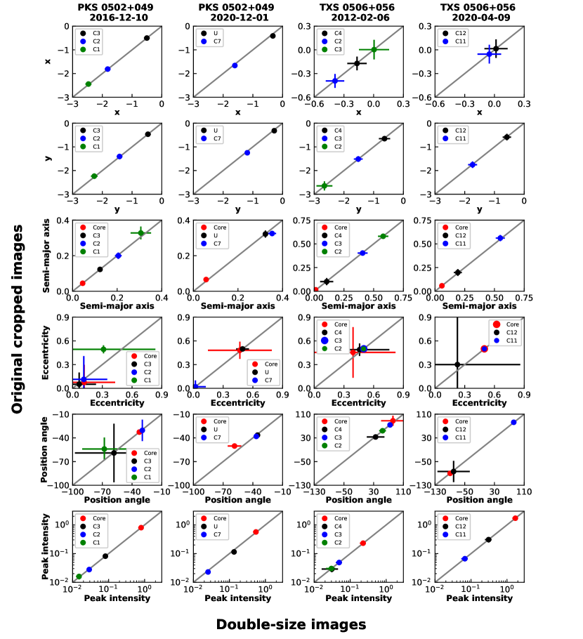
Figure 7: Comparison between the structural elliptical Gaussian parameters obtained from CE model-fittings for two images of PKS 0502+049 (first two columns from left to right) and two images of TXS 0506+056 (last two columns). Ordinate and abscissa axes correspond, respectively, to the values of the CE structural parameters obtained from the cropped images used in this work and from the new cropped images after doubling their original sizes. The Gaussian peak coordinates $x$ and $y$, as well as the semi-major axis are in units of milliarcseconds, while the structural position angle is given in degrees and the peak intensity (in logarithm scale) in units of Jy beam^-1. Error bars show the $1\sigma$ uncertainties of those quantities.

References

- Abraham (2000) Abraham Z., 2000, A&A, 355, 915
- Agudo et al. (2011) Agudo I., et al., 2011, ApJ, 735, L10
- Ansoldi et al. (2018) Ansoldi S., et al., 2018, ApJ, 863, L10
- Atwood et al. (2009) Atwood W. B., et al., 2009, ApJ, 697, 1071
- Atwood et al. (2013) Atwood W., et al., 2013, arXiv e-prints, p. arXiv:1303.3514
- Banik & Bhadra (2019) Banik P., Bhadra A., 2019, Phys. Rev. D, 99, 103006
- Banik et al. (2020) Banik P., Bhadra A., Pandey M., Majumdar D., 2020, Phys. Rev. D, 101, 063024
- Blasi et al. (2013) Blasi M. G., et al., 2013, A&A, 559, A75
- Britzen et al. (2018) Britzen S., et al., 2018, MNRAS, 478, 3199
- Britzen et al. (2019) Britzen S., et al., 2019, A&A, 630, A103
- Caproni & Abraham (2004a) Caproni A., Abraham Z., 2004a, MNRAS, 349, 1218
- Caproni & Abraham (2004b) Caproni A., Abraham Z., 2004b, ApJ, 602, 625
- Caproni et al. (2011) Caproni A., Monteiro H., Abraham Z., Teixeira D. M., Toffoli R. T., 2011, ApJ, 736, 68
- Caproni et al. (2014) Caproni A., Melo I. T. e., Abraham Z., Monteiro H., Roland J., 2014, MNRAS, 441, 187
- Caproni et al. (2017) Caproni A., Abraham Z., Motter J. C., Monteiro H., 2017, ApJ, 851, L39
- Cohen (1988) Cohen J., 1988, Statistical Power Analysis for the Behavioral Sciences. Lawrence Erlbaum Associates
- Cutini et al. (2014) Cutini S., et al., 2014, MNRAS, 445, 4316
- Drinkwater et al. (1997) Drinkwater M. J., et al., 1997, MNRAS, 284, 85
- Gajendran et al. (2021) Gajendran S., Yeh L.-C., Jiang I.-G., 2021, New Astron., 88, 101602
- Gao et al. (2017) Gao S., Pohl M., Winter W., 2017, ApJ, 843, 109
- Garrappa et al. (2019) Garrappa S., et al., 2019, ApJ, 880, 103
- Gower et al. (1982) Gower A. C., Gregory P. C., Unruh W. G., Hutchings J. B., 1982, ApJ, 262, 478
- He et al. (2018) He H.-N., Inoue Y., Inoue S., Liang Y.-F., 2018, arXiv e-prints, p. arXiv:1808.04330
- Heumann & Schomaker (2017) Heumann C., Schomaker M., 2017, Introduction to Statistics and Data Analysis: With Exercises, Solutions and Applications in R. Springer International Publishing, https://books.google.com.br/books?id=4mQBDgAAQBAJ
- Homan et al. (2003) Homan D. C., Lister M. L., Kellermann K. I., Cohen M. H., Ros E., Zensus J. A., Kadler M., Vermeulen R. C., 2003, ApJ, 589, L9
- Homan et al. (2006) Homan D. C., et al., 2006, ApJ, 642, L115
- Hovatta et al. (2020) Hovatta T., et al., 2020, arXiv e-prints, p. arXiv:2009.10523
- Hughes et al. (1985) Hughes P. A., Aller H. D., Aller M. F., 1985, ApJ, 298, 301
- IceCube Collaboration (2018) IceCube Collaboration 2018, Science, 361, 147
- IceCube Collaboration et al. (2018) IceCube Collaboration et al., 2018, Science, 361, eaat1378
- Johnston et al. (1995) Johnston K. J., et al., 1995, AJ, 110, 880
- Jones et al. (2000) Jones D. L., Wehrle A. E., Meier D. L., Piner B. G., 2000, ApJ, 534, 165
- Jorstad et al. (2001) Jorstad S. G., Marscher A. P., Mattox J. R., Aller M. F., Aller H. D., Wehrle A. E., Bloom S. D., 2001, ApJ, 556, 738
- Jorstad et al. (2017) Jorstad S. G., et al., 2017, ApJ, 846, 98
- Keivani et al. (2018) Keivani A., et al., 2018, ApJ, 864, 84
- Konigl (1981) Konigl A., 1981, ApJ, 243, 700
- Kovalev et al. (2005) Kovalev Y. Y., et al., 2005, AJ, 130, 2473
- Kudryavtseva et al. (2011) Kudryavtseva N. A., et al., 2011, A&A, 526, A51
- Kun et al. (2019) Kun E., Biermann P. L., Gergely L. Á., 2019, MNRAS, 483, L42
- Li et al. (2020) Li X., An T., Mohan P., Giroletti M., 2020, ApJ, 896, 63
- Liang et al. (2018) Liang Y.-F., He H.-N., Liao N.-H., Xin Y.-L., Yuan Q., Fan Y.-Z., 2018, arXiv e-prints, p. arXiv:1807.05057
- Lisakov et al. (2017) Lisakov M. M., Kovalev Y. Y., Savolainen T., Hovatta T., Kutkin A. M., 2017, MNRAS, 468, 4478
- Lister et al. (2009a) Lister M. L., et al., 2009a, AJ, 137, 3718
- Lister et al. (2009b) Lister M. L., et al., 2009b, AJ, 138, 1874
- Lister et al. (2018) Lister M. L., Aller M. F., Aller H. D., Hodge M. A., Homan D. C., Kovalev Y. Y., Pushkarev A. B., Savolainen T., 2018, ApJS, 234, 12
- Lister et al. (2019) Lister M. L., et al., 2019, ApJ, 874, 43
- Liu et al. (2019) Liu R.-Y., Wang K., Xue R., Taylor A. M., Wang X.-Y., Li Z., Yan H., 2019, Phys. Rev. D, 99, 063008
- Lobanov (2005) Lobanov A. P., 2005, arXiv e-prints, pp astro–ph/0503225
- Mannheim (1995) Mannheim K., 1995, Astroparticle Physics, 3, 295
- Marscher & Gear (1985) Marscher A. P., Gear W. K., 1985, ApJ, 298, 114
- Max-Moerbeck et al. (2014) Max-Moerbeck W., et al., 2014, MNRAS, 445, 428
- Mücke & Protheroe (2001) Mücke A., Protheroe R. J., 2001, Astroparticle Physics, 15, 121
- Murase (2017) Murase K., 2017, Active Galactic Nuclei as High-Energy Neutrino Sources. pp 15–31, doi:10.1142/9789814759410_0002
- Murase et al. (2018) Murase K., Oikonomou F., Petropoulou M., 2018, ApJ, 865, 124
- Neronov & Semikoz (2020) Neronov A., Semikoz D., 2020, arXiv e-prints, p. arXiv:2012.04425
- Otterbein et al. (1998) Otterbein K., Krichbaum T. P., Kraus A., Lobanov A. P., Witzel A., Wagner S. J., Zensus J. A., 1998, A&A, 334, 489
- Padovani et al. (2018) Padovani P., Giommi P., Resconi E., Glauch T., Arsioli B., Sahakyan N., Huber M., 2018, MNRAS, 480, 192
- Padovani et al. (2019) Padovani P., Oikonomou F., Petropoulou M., Giommi P., Resconi E., 2019, MNRAS, 484, L104
- Paiano et al. (2018) Paiano S., Falomo R., Treves A., Scarpa R., 2018, ApJ, 854, L32
- Petropoulou et al. (2020) Petropoulou M., et al., 2020, ApJ, 891, 115
- Plavin et al. (2019) Plavin A. V., Kovalev Y. Y., Pushkarev A. B., Lobanov A. P., 2019, MNRAS, 485, 1822
- Plavin et al. (2020) Plavin A., Kovalev Y. Y., Kovalev Y. A., Troitsky S., 2020, ApJ, 894, 101
- Plavin et al. (2021) Plavin A. V., Kovalev Y. Y., Kovalev Y. A., Troitsky S. V., 2021, ApJ, 908, 157
- Press et al. (1992) Press W. H., Teukolsky S. A., Vetterling W. T., Flannery B. P., 1992, Numerical recipes in C. The art of scientific computing
- Pushkarev et al. (2012) Pushkarev A. B., Hovatta T., Kovalev Y. Y., Lister M. L., Lobanov A. P., Savolainen T., Zensus J. A., 2012, A&A, 545, A113
- Readhead (1994) Readhead A. C. S., 1994, ApJ, 426, 51
- Reimer et al. (2019) Reimer A., Böttcher M., Buson S., 2019, ApJ, 881, 46
- Richards et al. (2014) Richards J. L., Hovatta T., Max-Moerbeck W., Pavlidou V., Pearson T. J., Readhead A. C. S., 2014, MNRAS, 438, 3058
- Rodrigues et al. (2018) Rodrigues X., Fedynitch A., Gao S., Boncioli D., Winter W., 2018, ApJ, 854, 54
- Rodrigues et al. (2019) Rodrigues X., Gao S., Fedynitch A., Palladino A., Winter W., 2019, ApJ, 874, L29
- Roland et al. (2013) Roland J., Britzen S., Caproni A., Fromm C., Glück C., Zensus A., 2013, A&A, 557, A85
- Romero et al. (2000) Romero G. E., Chajet L., Abraham Z., Fan J. H., 2000, A&A, 360, 57
- Ros et al. (2020) Ros E., Kadler M., Perucho M., Boccardi B., Cao H. M., Giroletti M., Krauß F., Ojha R., 2020, A&A, 633, L1
- Rubinstein (1997) Rubinstein R. Y., 1997, European Journal of Operational Research, 99, 89
- Sahakyan (2018) Sahakyan N., 2018, The Astrophysical Journal, 866, 109
- Sahakyan (2019) Sahakyan N., 2019, A&A, 622, A144
- Shepherd (1997) Shepherd M. C., 1997, in Hunt G., Payne H., eds, Astronomical Society of the Pacific Conference Series Vol. 125, Astronomical Data Analysis Software and Systems VI. p. 77
- Stecker et al. (1991) Stecker F. W., Done C., Salamon M. H., Sommers P., 1991, Phys. Rev. Lett., 66, 2697
- Türler et al. (2000) Türler M., Courvoisier T. J. L., Paltani S., 2000, A&A, 361, 850
- Urry & Padovani (1995) Urry C. M., Padovani P., 1995, PASP, 107, 803
- Valtaoja et al. (1992) Valtaoja E., Terasranta H., Urpo S., Nesterov N. S., Lainela M., Valtonen M., 1992, A&A, 254, 71
- Wasserman (2010) Wasserman L., 2010, All of Statistics: A Concise Course in Statistical Inference. Springer Publishing Company, Incorporated
- Xue et al. (2020) Xue R., Liu R.-Y., Wang Z.-R., Ding N., Wang X.-Y., 2020, arXiv e-prints, p. arXiv:2011.03681
- Zhang et al. (2020) Zhang B. T., Petropoulou M., Murase K., Oikonomou F., 2020, ApJ, 889, 118