Pluto’s atmosphere in plateau phase since 2015 from a stellar occultation at Devasthal

Abstract

A stellar occultation by Pluto was observed on 6 June 2020 with the 1.3-m and 3.6-m telescopes located at Devasthal, Nainital, India, using imaging systems in the I and H bands, respectively. From this event, we derive a surface pressure for Pluto’s atmosphere of $p_{\rm surf}=12.23^{+0.65}_{-0.38}$ $\mu$bar. This shows that Pluto’s atmosphere is in a plateau phase since mid-2015, a result which is in excellent agreement with the Pluto volatile transport model of Meza et al. (2019). This value does not support the pressure decrease reported by independent teams, based on occultations observed in 2018 and 2019, see Young et al. (2021) and Arimatsu et al. (2020), respectively.

1 Introduction

Owing to its high obliquity (120^∘) and high orbital eccentricity (0.25), Pluto suffers intense seasonal episodes. Its poles remain, for decades, in permanent sunlight or darkness over its 248-year heliocentric revolution. This leads to strong effects on its N₂ atmosphere that is mainly controlled by vapor pressure equilibrium with the surface N₂ ice. The NASA New Horizons flyby in July 2015 revealed a large depression, Sputnik Planitia, filled by N₂ ice (Stern et al., 2015), which appeared to be the main engine that controls the seasonal variation of atmospheric pressure during one seasonal cycle (Bertrand & Forget, 2016; Bertrand et al., 2018; Johnson et al., 2021). Apart from these crucial results, a comprehensive review of the composition, photochemistry, atmospheric dynamics, circulation and escape processes derived from the New Horizons data is presented in Gladstone & Young (2019).

In parallel, ground-based observations of stellar occultations allowed various teams to accurately monitor Pluto’s atmospheric pressure since 1988. A compilation of twelve occultations observed between 1988 and 2016 shows a three-fold monotonic increase of pressure during this period, that can be explained by the progression of summer over the northern hemisphere, exposing Sputnik Planitia to the solar radiation (Meza et al., 2019). This increase can be explained consistently by a Pluto volatile transport model, which predicts that the pressure should peak around 2020. A gradual decline should then last for two centuries under the combined effects of Pluto’s recession from the Sun and the prevalence of the winter season over Sputnik Planitia.

Here we present the results of a stellar occultation by Pluto that occurred on 6 June 2020. It was observed in the near-infrared by two large telescopes at the Devasthal station, Nainital, India. The high signal-to-noise ratio light curves obtained with these instruments allow us to derive an accurate value of Pluto’s atmospheric pressure, using the same approach as in Dias-Oliveira et al. (2015) and Meza et al. (2019). This occultation was particularly timely as it can test the validity of the current models of Pluto’s atmosphere evolution. Moreover, as Pluto is now moving away from the Galactic plane as seen from Earth, stellar occultations by the dwarf planet are becoming increasingly rare, making this event a decisive one.

2 Observations and Data Analysis

2.1 Occultation

The 6 June 2020 occultation campaign was organized within the Lucky Star project. The prediction used the Gaia DR2 position at epoch of occultation (Table 1) and the NIMAv8/PLU055 Pluto’s ephemeris derived from previous occultations observed since 1988 (Desmars et al., 2019). More information on the event (shadow path, charts, photometry, etc.) is available in a dedicated web page.

The event was successfully recorded in the I and H bands using the 1.3-m Devasthal Fast Optical Telescope (DFOT) and the 3.6-m Devasthal Optical Telescope (DOT), respectively. The I and H band magnitudes of the occulted star are $\sim$12.3 and 11.6, respectively, while that of Pluto during the epoch of occultation were $\sim$13.8 and 13.3, respectively. Thus, the occulted star was more than 1.5 mag brighter than the combined Pluto + Charon system, ensuring a high contrast event, i.e. a significant drop of the total flux, which combines the fluxes from the star, Pluto and Charon.

Both telescopes are operated by the Aryabhatta Research Institute of Observational Sciences (ARIES) located at Nainital, India. Observations were also planned with the 2-m Himalayan Chandra Telescope (HCT), Hanle, operated by the Indian Institute of Astrophysics, Bangalore, India. However, the event was clouded out at that site.

The event was observed in the I-band with DFOT-Andor DZ436 camera (2048$\times$2048-pixel; plate scale $\sim$0.5 arcsec/pixel). The central 401$\times$401 pixel region was used in 2$\times$2 binning mode. With a readout rate of 1 MHz, shift speed of 16 $\mu$s and exposure time of 1.7-s, a total cycle time of 2.507-s was achieved. The final acquired image was a FITS data cube of 600 frames. A simultaneous observation was carried out with DOT in the H-band with the TIRCAM2 instrument (Naik et al., 2012; Baug et al., 2018), an imaging camera housing a cryo-cooled Raytheon InSb Aladdin III Quadrant focal plane infrared array (512$\times$512-pixel; plate scale = 0.167 arcsec/pixel). The full frame was used with a readout rate of 1 MHz, exposure time of 5 s, and total cycle time of 5.336 s. The final acquired image was a FITS data cube of 255 frames.

From the light curve fitting described below, we reconstructed Pluto’s shadow path on Earth and the geometry of the occultation (Fig. 1). Note in this figure that two stellar images (primary and secondary, see Sicardy et al. 2016) actually scanned Pluto’s limb. However, the flux of the secondary image was always fainter than that of the primary by a factor larger than 25, making it negligible in our case. Consequently, this event essentially scanned the northern, summer hemisphere of Pluto.

Table 1: Circumstances of observations, adopted parameters and result of the atmospheric fit.

Observation log
3.6-m (DOT)
Coordinates, altitude	79∘ 41′ 3.6′′ E, 29∘ 21′ 39.4′′ N, 2450 m
Camera	TIRCAM2 Raytheon InSb array
Filter ($\lambda/\Delta\lambda$, $\mu$m)	H (1.60/0.30)
Exposure time/Cycle time (s)	5./5.336
1.3-m (DFOT)
Coordinates, altitude	79∘ 41′ 6.1′′ E, 29∘ 21′ 41.5′′ N, 2450 m
Camera	ANDOR DZ436
Filter ($\lambda/\Delta\lambda$, $\mu$m)	I (0.85/0.15)
Exposure time/Cycle time (s)	1.7/2.507
Occulted star
Identification (Gaia DR2)	6864932072159710592
J2000 position at epoch (ICRF)	$\alpha=19^{\rm h}45^{\rm m}33.9079^{\rm s}$, $\delta=-22^{\circ}10^{\prime}19.128^{\prime\prime}$
Pluto’s body
Mass1	$GM_{P}=8.696\times 10^{11}$ m3 sec-2
Radius1	$R_{P}=1187$ km
Geocentric distance	$4.97407\times 10^{9}$ km
Pluto’s atmosphere
N2 molecular mass	$\mu=4.652\times 10^{-26}$ kg
N2 molecular	$K=1.091\times 10^{-23}$
Refractivity2	$+6.282\times 10^{-26}/\lambda_{\rm\mu m}^{2})$ cm3 molecule-1
Boltzmann constant	$k=1.380626\times 10^{-23}$ J K-1
Results of atmospheric fit (with 1$\sigma$ error bars)
Pressure at radius 1215 km	$p_{\rm 1215}=6.655^{+0.35}_{-0.21}$ $\mu$bar
Surface pressure3	$p_{\rm surf}=12.23^{+0.65}_{-0.38}$ $\mu$bar
Closest approach distance of Devasthal to shadow center4	$\rho_{\rm C/A,D}=-735^{+7}_{-15}$ km
Closest approach time of Devasthal to shadow center	$t_{\rm C/A,D}$= 19:02:43.0$\pm$0.14 s UT
Geocentric closest approach distance to shadow center4	$\rho_{\rm C/A,G}=+6044^{+15}_{-7}$ km
Geocentric closest approach time to shadow center5	$t_{\rm C/A,G}$= 19:01:01.7$\pm$0.14 s UT

Note. — ¹Stern et al. (2015), where $G$ is the constant of gravitation. ²Washburn (1930), where $\lambda_{\rm\mu m}$ is the wavelength expressed in microns. ³Using a ratio $p_{\rm surf}/p_{\rm 1215}=1.837$ given by the template model Meza et al. (2019). ⁴Negative (resp. positive) values mean that the point considered went south (resp. north) of the shadow center. ⁵Although the quoted error bar is small, a systematic error of about 1 s may be present in $t_{\rm C/A,G}$, see text.

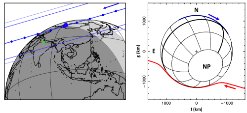
Figure 1: Left: The reconstructed shadow path of Pluto on 6 June 2020. The blue dots on the shadow central line are plotted every minute. The larger one marks the Geocentric closest approach at 19:01:01.7 UT, and the arrow indicates the direction of motion. The green dot is Devasthal’s position. The dark and light blue lines on each side of centrality correspond to the stellar half-light level and 1% stellar drop level (the practical detection limit), respectively. The dark gray region is for astronomical night (Sun more than 18 deg below the horizon), while the light gray region is for astronomical twilight (Sun between 0 and 18 deg below the horizon). Right: Geometry of the 6 June 2020 stellar occultation event. Pluto’s orientation is shown at 19:02 UT. The thicker lines are the equator and the prime (Charon-facing) meridians, respectively. The letters N, E and NP indicate the celestial north, celestial east and Pluto’s north pole, respectively. The red and the blue lines represent, respectively, the motion of the primary and secondary stellar images relative to Pluto, as seen from Devasthal, see text for details. The quantities $f$ and $g$ are the offsets of the stellar images with respect to Pluto’s center, marked with a ‘+’ symbol.

2.2 Light curve fitting

The observed datasets were fitted with synthetic light curves using the method described in Dias-Oliveira et al. (2015), in particular with the same template temperature profile, $T(r)$, where $r$ is the distance to Pluto’s center. The approach involves the simultaneous fitting of the observed refractive occultation light curves by synthetic profiles that are generated by a ray-tracing code that uses the Snell–Descartes law. The various parameters used in our fitting procedure are listed in Table 1.

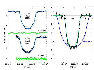
Figure 2: Left: The blue curves are a simultaneous fit to our 6 June 2020 Pluto occultation light curves (black squares) obtained with the 3.6-m and 1.3-m telescopes of ARIES at Desvasthal, over a 320-s interval bracketing the event. The residuals (observation-minus-model) are plotted in green below each light curve. The parameters of the best atmospheric model are listed in Table 1. The value of $\chi^{2}_{\rm dof}$, the $\chi^{2}$ per degree of freedom for each fit, is displayed at the lower right corner of each light curve. The lower and upper horizontal lines are the normalized total flux (star+Pluto+Charon) and the zero flux levels, respectively. The 3.6-m light curve has been shifted vertically by +1.2 for better viewing. Right: Black bullets are the data points obtained at the Karaj station during the same occultation event, and the black line is the associated best fitting model from Poro et al. (2021) (credit: A&A 653, L7, 2021, reproduced by permission ©ESO). The blue curve is our expected light curve at Karaj using the results of Poro et al. (2021), i.e. $p_{\rm surf}=12.36$ $\mu$bar and a closest approach distance to Pluto’s shadow at that station of 605.3 km. It shows a large discrepancy by a factor of about two in the time scale when compared with the expected light curve. Assuming a timing problem at Karaj, and trying to superimpose our synthetic curves, we obtain a significant discrepancy at the bottom of the occultation light curve between our model (green curve) and and the model of Poro et al. (2021). This reveals an inconsistency between the ray tracing approach adopted by us and by Poro et al. (2021).

There are $M=4$ adjusted parameters in our model: (1) $p_{\rm surf}$, the pressure at Pluto’s surface, (2) $\Delta\rho$, the cross-track offset to Pluto’s ephemeris, and (3-4) the two Pluto+Charon’s contributions $\phi_{0}$ to each of the two ARIES light curves. Owing to less than optimal sky conditions prevailing, observations to separately measure the occulted star and Pluto’s system the nights prior to or after the event was not possible. Due to this unavailability of calibration data, the $\phi_{0}$’s in our analysis are not known.

There is a fifth adjusted parameter which is completely uncorrelated with the other four, the time shift, $\Delta t$, that needs to be applied to Pluto’s ephemeris to best fit the data. This parameter accounts for the ephemeris offset to apply along Pluto’s apparent motion and for errors in the star position. It finally provides, $t_{\rm C/A,G}$, the time of closest approach of Pluto to the star in the sky plane, as seen from the Geocenter, see Table 1.

When fitting the two Devasthal light curves, a discrepancy of 2.4 s appeared in the best-fitting $\Delta t$ derived from each telescope, thus revealing a problem in the recording of the absolute times at one (or both) telescopes. Since it is difficult to decipher the origin of this discrepancy, any attempt to correct for the same would be futile. Hence, we have chosen to apply independent $\Delta t$ to each telescope, and calculate the final $t_{\rm C/A,G}$ as an average of the two obtained values, weighted by the quality of the two light curves (measured by the noise in the data). With this approach, although the internal error bar on $t_{\rm C/A,G}$ is small ($\pm$0.14 s, Table 1), a systematic uncertainty of the order of 1 s still remains in the quoted value of $t_{\rm C/A,G}$.

The best fit to the data are shown in Fig 2. The function $\chi^{2}~{}=~{}\sum_{1}^{N}~{}[(\phi_{\rm i,obs}-\phi_{\rm i,syn})/\sigma_{i}]^{2}$ was used to assess the quality of the fit, where $\sigma_{i}$ reflects the noise level of each of the $N=362$ data points, and $\phi_{\rm i,obs}$ and $\phi_{\rm i,syn}$ are the observed and synthetic fluxes at the $i^{\rm th}$ data point, respectively. Satisfactory fits are obtained for a $\chi^{2}$ value per degree of freedom $\chi^{2}_{\rm dof}=\chi^{2}_{\rm min}/(N-M)\sim 1$, where $\chi^{2}_{\rm min}$ is the minimum value of $\chi^{2}$ obtained in the fitting procedure. This is the case here, with individual values $\chi^{2}_{\rm dof}=0.984$ and $\chi^{2}_{\rm dof}=1.07$ at DOT and DFOT, respectively, and a global value $\chi^{2}_{\rm dof}=1.03$ corresponding to the simultaneous fit to the two light curves.

Our fit is mainly sensitive to regions above 30 km altitude, so our primary result is the pressure near the radius 1215 km, $p_{1215}=6.665^{+0.35}_{-0.21}$ $\mu$bar (Table 1). A factor of 1.837 is then applied to convert this into $p_{\rm surf}$, see Meza et al. (2019). Fig. 3 shows the $\chi^{2}$ map plotted as a function of the two parameters $p_{\rm surf}$ and $\Delta\rho$. Note that because there is only one occultation chord at hand (Fig. 1), a correlation between $p_{\rm surf}$ and $\Delta\rho$ is observed. Using the $\chi_{\rm min}^{2}+1$ criterion, we obtain the best-fitting value of $p_{\rm surf}=12.23^{+0.65}_{-0.38}$ $\mu$bar. The marginal error bar quoted here is estimated by ignoring the value of $\Delta\rho$.

Besides the observations presented here, the 6 June 2020 event was observed by an independent team, see Poro et al. (2021). The event was observed at low elevation (6 degrees) near the city of Karaj in Iran with a 60-cm telescope. The authors mention that they use the ray-tracing method of Dias-Oliveira et al. (2015), i.e. a procedure that should be fully consistent with our own approach.

However, their derived value $p_{\rm surf}=12.36\pm 0.38$ $\mu$bar, is questionable. First, the time axis for the Karaj light curve in Poro et al. (2021) is wrong by a large factor of about two, see Fig. 2. This makes impossible to obtain any realistic value of $p_{1215}$ from this light curve. Secondly, assuming that the Karaj time axis has some (undocumented) problems, considering the occultation geometry at that station and adopting the $p_{1215}=6.72$ $\mu$bar value of Poro et al. (2021), we generated a synthetic model using our own ray-tracing code. By shrinking the time scale in an attempt to superimpose our model (green curve in Fig. 2) onto the results of Poro et al. (2021) (black curve), we see a clear discrepancy between our models in the deepest part of the occultation. This shows that the ray tracing code of Poro et al. (2021) is inconsistent with ours. Consequently, the results of Poro et al. (2021) are impossible to obtain considering their published light curve, and probably stems from improper use of their ray-tracing code. Finally, we note that the error bar for $p_{\rm surf}$ is inconsistent with the error bar that the authors obtain for the pressure at radius 1215 km, $p_{1215}=6.72\pm 0.48$ $\mu$bar, see their Fig. 3. As the error bar scales like the value of the pressure, the error bar for the surface pressure should be $\pm 0.88$ $\mu$bar, not $\pm 0.38$ $\mu$bar.

3 Pressure evolution

In Figure 3, we plot our measurement of $p_{\rm surf}$ in 2020 (red point) along with other published values (Hinson et al., 2017; Meza et al., 2019; Arimatsu et al., 2020; Young et al., 2021). The 6 June 2020 occultation shows that the pressure increase prevailing between 1988 and 2013 stopped, and reached a stationary regime since 2015. This is in line with the Pluto volatile transport model described in Meza et al. (2019).

Our results do not support the rapid pressure decrease claimed by Arimatsu et al. (2020) (who also used the ray-tracing method of Dias-Oliveira et al. 2015) from an occultation observed on 17 July 2019, see the point ‘A20’ in Fig. 3. With closest approach to Pluto’s shadow center of 1008 km, the work of Arimatsu et al. (2020) is based on an occultation that was more grazing than the event reported here (with closest approach of 735 km). This induces a larger correlation between the parameters $p_{\rm surf}$ and $\Delta\rho$. In particular, Arimatsu et al. (2020) mention that the pressure drop they find between 2016 and 2019 is actually detected at the 2.4$\sigma$ level, and thus remains marginally significant. We thus estimate that the 2019 data point lacks accuracy to claim that a large decrease occurred in 2019, followed by a return to a pressure close to that of 2015 during the year 2020 (this work).

We do not confirm either the decrease of pressure reported by Young et al. (2021), based on the 15 August 2018 occultation observed from about two dozen stations in USA and Mexico, from which Young et al. (2021) derive a value $p_{\rm surf}=11.13\pm 0.4$ $\mu$bar (the point ‘Y21’ in Fig. 3), using a method that is not described by these authors.

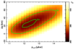
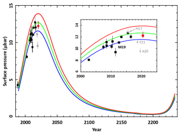
Figure 3: Left: The $\chi^{2}$ map used to derived the best-fitting surface pressure ($p_{\rm surf}$) and the cross-track correction to the ephemeris ($\Delta\rho$). The inner and outer green lines delimit the respective 1$\sigma$ and 3$\sigma$ error domains, see text for details. Right: Evolution of Pluto’s atmospheric pressure between 1988 and 2020. All the error bars are displayed at 1$\sigma$ level. Some point do not show error bars because they are smaller than the squares. The black points are the values published by Meza et al. (2019) (M19) and the red point is the result of the present work, as derived from the left panel. The gray points are from other works. In chronological order, they are: H17, the New Horizons value from the radio science data occultation (ingress point, 14 July 2015, Hinson et al. 2017). Note that this point is superimposed onto our own point of 29 June 2015; Y21, the value derived by Young et al. (2021) from the ground-based, multi-chord 15 August 2018 occultation; and A20, the result of Arimatsu et al. (2020) obtained from a grazing, single-chord occultation observed on 17 July 2019. The colored lines are the modeled annual evolution of the surface pressure obtained with the Pluto volatile transport model described in Meza et al. (2019). The blue, green and red curves correspond to N₂ ice albedos of 0.73, 0.725 and 0.72, respectively.

It is important to note that all the points derived by us between 2002 and 2020 (Meza et al. 2019 and present work) are obtained using a unique template temperature profile $T(r)$. This assumption is backed up by the fact that although the pressure increased by a factor of about three between 1988 and 2016 (Meza et al., 2019), the retrieved temperature profiles in 1988, 2002, 2012 and 2015 (Yelle & Elliot, 1997; Hinson et al., 2017; Sicardy et al., 2003; Young et al., 2008; Dias-Oliveira et al., 2015, respectively) are all similar, with a strong positive thermal gradient in the lower part of the atmosphere that peaks at $T\sim 110$ K near $r=1215$ km, followed by a roughly isothermal upper branch with a mild negative thermal gradient. This globally fits the methane-thermostat model of Yelle & Lunine (1989), where the upper-atmosphere temperature is robustly maintained near 100 K through the radiative properties of atmospheric CH4, almost independently of its abundance, while the lower part is forced by heat conduction with the cold surface near 38 K. So even if small systematic errors are introduced at this stage, a consistent comparison using a constant $T(r)$ between events is possible, so that general trends on pressure evolution can be monitored. Thus, at this stage, the methodologies used by both Arimatsu et al. (2020) and Young et al. (2021) should be compared with ours in some well-defined test cases to see if our approaches are consistent, and thus, fully comparable.

Note that our results could be compared with those of New Horizons, derived from the radio occultation experiment (REX) in July 2015. Values of $p_{\rm surf}=12.8\pm 0.7$ and $10.2\pm 0.7$ $\mu$bar at entry and exit, respectively, were obtained (Hinson et al., 2017). The difference between the two values can be attributed to a 5 km difference in radius at the two locations probed by REX, the lower value at exit corresponding to higher terrains on Pluto. As the entry value probed a point over Sputnik Planitia, where sublimation of N₂ takes place, it should be more representative of $p_{\rm surf}$ than the exit value. We see that our value of $p_{\rm surf}=12.71\pm 0.14$ $\mu$bar derived from the 29 June 2015 occultation (Meza et al., 2019) is in excellent agreement with the REX value of July 2015 (point ‘H17’ in Fig. 3), giving confidence that our approach not only provides general trends, but also good estimates of $p_{\rm surf}$.

4 Conclusions

The 6 June 2020 stellar occultation allowed us to constrain Pluto’s atmospheric evolution. The surface pressure that we obtain, $p_{\rm surf}=12.23^{+0.65}_{-0.38}$ $\mu$bar, shows that Pluto’s atmosphere has reached a plateau since mid-2015, a result which is in line with the Pluto volatile transport model discussed in Meza et al. (2019). Our result does not support the drops of pressure reported by Young et al. (2021) and Arimatsu et al. (2020) in 2018 and 2019, respectively. These inconsistencies call for careful comparisons between methodologies before any conclusions based on independent teams be drawn.

We note that if the model presented in Meza et al. (2019) is correct, and considering the typical error bars derived from occultations, it will be difficult to firmly confirm a pressure drop before 2025. Meanwhile, observations should be organized whenever possible, as unaccounted processes may cause pressure changes not predicted by models.

References

- Arimatsu et al. (2020) Arimatsu, K., Hashimoto, G. L., Kagitani, M., et al. 2020, Astron. Astrophys., 638, L5, doi: 10.1051/0004-6361/202037762
- Baug et al. (2018) Baug, T., Ojha, D. K., Ghosh, S. K., et al. 2018, Journal of Astronomical Instrumentation, 7, 1850003, doi: 10.1142/S2251171718500034
- Bertrand & Forget (2016) Bertrand, T., & Forget, F. 2016, Nature, 540, 86, doi: 10.1038/nature19337
- Bertrand et al. (2018) Bertrand, T., Forget, F., Umurhan, O. M., et al. 2018, Icarus, 309, 277, doi: 10.1016/j.icarus.2018.03.012
- Desmars et al. (2019) Desmars, J., Meza, E., Sicardy, B., et al. 2019, Astron. Astrophys., 625, A43, doi: 10.1051/0004-6361/201834958
- Dias-Oliveira et al. (2015) Dias-Oliveira, A., Sicardy, B., Lellouch, E., et al. 2015, ApJ, 811, 53, doi: 10.1088/0004-637X/811/1/53
- Gladstone & Young (2019) Gladstone, G. R., & Young, L. A. 2019, Annual Review of Earth and Planetary Sciences, 47, 119, doi: 10.1146/annurev-earth-053018-060128
- Hinson et al. (2017) Hinson, D. P., Linscott, I. R., Young, L. A., et al. 2017, Icarus, 290, 96, doi: 10.1016/j.icarus.2017.02.031
- Johnson et al. (2021) Johnson, P. E., Keane, J. T., Young, L. A., & Matsuyama, I. 2021, \psj, 2, 194, doi: 10.3847/PSJ/ac1d42
- Meza et al. (2019) Meza, E., Sicardy, B., Assafin, M., et al. 2019, Astron. Astrophys., 625, A42, doi: 10.1051/0004-6361/201834281
- Naik et al. (2012) Naik, M. B., Ojha, D. K., Ghosh, S. K., et al. 2012, Bulletin of the Astronomical Society of India, 40, 531. https://arxiv.org/abs/1211.5542
- Poro et al. (2021) Poro, A., Ahangarani Farahani, F., Bahraminasr, M., et al. 2021, A&A, 653, L7, doi: 10.1051/0004-6361/202141718
- Sicardy et al. (2003) Sicardy, B., Widemann, T., Lellouch, E., et al. 2003, Nature, 424, 168, doi: 10.1038/nature01766
- Sicardy et al. (2016) Sicardy, B., Talbot, J., Meza, E., et al. 2016, Astrophys. J., Lett., 819, L38, doi: 10.3847/2041-8205/819/2/L38
- Stern et al. (2015) Stern, S. A., Bagenal, F., Ennico, K., et al. 2015, Science, 350, aad1815, doi: 10.1126/science.aad1815
- Washburn (1930) Washburn, E. W. 1930, International Critical Tables of Numerical Data: Physics, Chemistry and Technology. (Vol. 7, McGraw-Hill, New York, 1930)
- Yelle & Elliot (1997) Yelle, R. V., & Elliot, J. L. 1997, Atmospheric Structure and Composition: Pluto and Charon, ed. S. A. Stern & D. J. Tholen, 347
- Yelle & Lunine (1989) Yelle, R. V., & Lunine, J. I. 1989, Nature, 339, 288, doi: 10.1038/339288a0
- Young et al. (2021) Young, E., Young, L. A., Johnson, P. E., & PHOT Team. 2021, in AAS/Division for Planetary Sciences Meeting Abstracts, Vol. 53, AAS/Division for Planetary Sciences Meeting Abstracts, 307.06
- Young et al. (2008) Young, E. F., French, R. G., Young, L. A., et al. 2008, AJ, 136, 1757, doi: 10.1088/0004-6256/136/5/1757