Phase Transitions in High Purity Zr Under Dynamic Compression

Abstract

We present results from ramp compression experiments on high-purity Zr that show the $\alpha\rightarrow\omega$, $\omega\rightarrow\beta$, as well as reverse $\beta\rightarrow\omega$ phase transitions. Simulations with a multi-phase equation of state and phenomenological kinetic model match the experimental wave profiles well. While the dynamic $\alpha\rightarrow\omega$ transition occurs $\sim 9$ GPa above the equilibrium phase boundary, the $\omega\rightarrow\beta$ transition occurs within 0.9 GPa of equilibrium. We estimate that the dynamic compression path intersects the equilibrium $\omega-\beta$ line at $P=29.2$ GPa, and $T=490$ K. The thermodynamic path in the interior of the sample lies $\sim 100$ K above the isentrope at the point of the $\omega\rightarrow\beta$ transition. Approximately half of this dissipative temperature rise is due to plastic work, and half is due to the non-equilibrium $\alpha\rightarrow\omega$ transition. The inferred rate of the $\alpha\rightarrow\omega$ transition is several orders of magnitude higher than that measured in dynamic diamond anvil cell (DDAC) experiments in an overlapping pressure range. We discuss a model for the influence of shear stress on the nucleation rate. We find that the shear stress $s_{ji}$ has the same effect on the nucleation rate as a pressure increase $\delta P=c\epsilon_{ij}s_{ji}/(\Delta V/V),$ where $c$ is a geometric constant $\sim 1$ and, $\epsilon_{ij}$ are the transformation shear strains. The small fractional volume change $\Delta V/V\approx 0.1$ at the $\alpha\rightarrow\omega$ transition amplifies the effect of shear stress, and we estimate that for this case $\delta P$ is in the range of several GPa. Correcting our transition rate to a hydrostatic rate brings it approximately into line with the DDAC results, suggesting that shear stress plays a significant role in the transformation rate.

I Introduction

Metallic Zr and its alloys have practical applications in chemical processing and nuclear power.Northwood (1985) The high pressure properties and phase diagram of pure Zr have been studied extensively Greeff et al. (2004); Greeff (2005); Liu et al. (2008); Dewaele et al. (2016); Zilbershteyn et al. (1973); Zhang et al. (2005); Akahama et al. (1991); Xia et al. (1990, 1991); Ono and Kikegawa (2015); Cerreta et al. (2005); Rigg et al. (2009); Jacobsen et al. (2015); Errandonea et al. (2005); Zhao et al. (2005) using both static and dynamic compression techniques. The high pressure phase diagram is shown in figure 2. The ambient pressure $\alpha$ phase has the hcp structure. The $\beta$ phase, with bcc structure appears at high temperature and high pressure. The $\omega$ phase, with a hexagonal structure with 3 atoms per cell, occupies intermediate $T$ and $P$. The sequence of phases with increasing pressure on the room $T$ isotherm, isentrope, and Hugoniot is $\alpha-\omega-\beta$. Dynamic compression studies Marsh (1980); Cerreta et al. (2005); Rigg et al. (2009); Gorman et al. (2020); Radousky et al. (2020); Kalita et al. (2020) have for the most part been focused on shock compression to measure the Hugoniot and investigate the $\alpha-\omega$, $\alpha-\beta$, and melting transitions.

In shock compression, an abrupt shock wave is driven through the sample, typically by a high velocity impact. In contrast, ramp compression Hawke et al. (1972); Hall et al. (2001) is achieved by a smoothly varying pressure wave. Ramp compression is less dissipative than shock compression, allowing investigation of the equation of state (EOS) and phase transitions at lower temperatures than shock loading. Under shock loading, a phase transition will not be evident in the wave profile if the shock pressure is too high so that the transition is overdriven. This is illustrated in figure 3 of ref. Rigg et al., 2009. Under ramp compression, transitions do not become overdriven. Any phase change encountered on the compression path should leave an imprint on the wave profile.

Here we present new ramp compression data on Zr, obtained via magnetic drive on the Z machine. We employ simulations using a multi-phase equation of state Greeff (2005) together with a phenomenological kinetic model Greeff (2016) to interpret these experiments together with shock loading data.Rigg et al. (2009) Our simulations agree well with experimental velocity profiles $v(t)$ measured at the sample window interface for both ramp and shock compression. Consistent with earlier workRigg et al. (2009); Greeff et al. (2004) we find strong kinetic effects on the $\alpha-\omega$ transition. The non-equilibrium transition contributes significantly to the dissipative heating during ramp compression. The Z-machine data shows the higher pressure $\omega-\beta$ transition in both the forward and reverse directions. This transition occurs closer to equilibrium than the $\alpha-\omega$ transition. The presence of the forward and reverse transitions allows us to refine the equilibrium phase diagram. Comparing the $\alpha-\omega$ transformation rates inferred from dynamic compression with those measured in a dynamic diamond anvil cell (DDAC)Jacobsen et al. (2015) shows the dynamic compression rate to be orders of magnitude higher that that in the DDAC in an overlapping pressure range. We consider a model for the influence of shear stress on the nucleation rate, and find that it is of the correct magnitude to explain the difference.

II Experiments

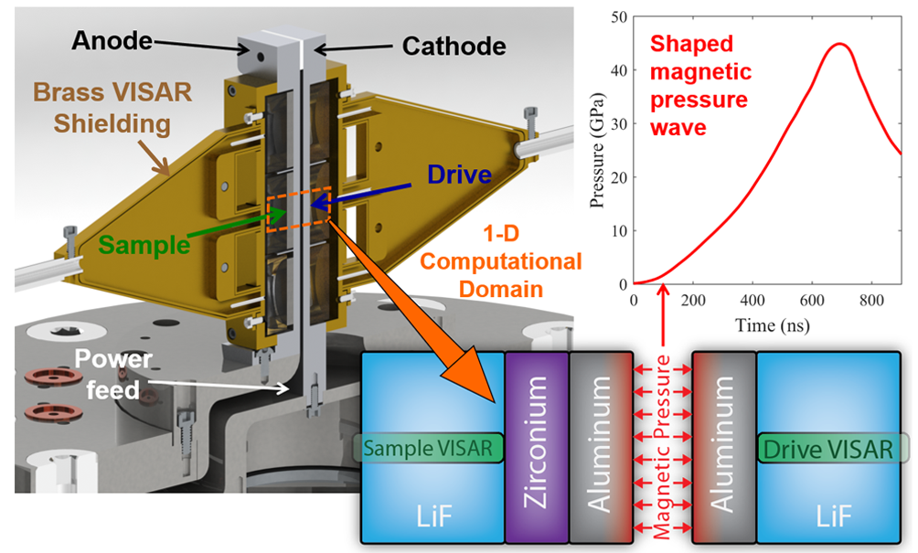
Figure 1: Configuration for the magnetic ramp compression experiments. Each drive/sample pair is analyzed independently through a set 1-D simulations where the magnetic pressure boundary condition is inferred from the drive measurement which then enables simulations of the zirconium sample side.

The experimental configuration for the ramp compression experiment, Z2913, is summarized in Figure 1. The geometry shown is referred to as a stripline Lemke et al. (2011) and consists of two parallel aluminum electrodes which are 2 mm thick separated by a gap of 1 mm. From top to bottom, three Zr samples with thicknesses of 1.01, 1.25, and 1.51 mm are glued to the anode electrode with angstrom bond; glue thicknesses are estimated to be on the order of 1 $\mu m$. The Zr samples are then backed with optically transparent 6 mm thick [100] LiF crystals using similar bonding characteristics. The LiF serves as a tamper which maintains the pressure at this interface and allows for a measurement of the unloading response and phase reversion. On the opposite side of the gap, the LiF is bonded directly to the electrode. In both cases, a 3 mm diameter Al spot coating $\sim$1 nm thick is deposited on the bonded side of the LiF giving a reflecting surface for the VISAR Barker and Hollenbach (1972) diagnostic. VISAR provides the velocity-time history at each of these interfaces and is the primary experimental observable.

The configuration shown in Figure 1 is ideal for performing high-fidelity simulations, which is key for the interpretation in this work. The cathode measurement represents the velocity at the Al/LiF interface and is referred to as the drive measurement because it allows for direct quantification of the magnetic pressure applied to the electrodes. This quantification is known as an unfold Lemke et al. (2003) and consists of solving for the pressure-time history such that 1-D hydrocode simulations of the drive configuration reproduce the measured velocity. Thus, it is assumed the Al and LiF are well known standards; the material models are described in detail in ref. Brown et al., 2014. Conventionally, unfolds are performed through magneto-hydrodynamics (MHD) simulations to solve for the magnetic field, but for this experiment the magnetic effects are negligible and a pressure boundary condition is sufficient. The pressure drive is preferred here for simplicity and compatibility with the research code containing phase transition kinetics model. As suggested by the 1-D computational domain in Figure 1, the benefit of this symmetric experimental configuration is the magnetic pressure must be the same across the electrode gap for a fixed height. Thus, once the pressure is determined for each drive measurement the only unknown in a simulation of the sample side is the Zr material model. These Zr models and their parameterizations are described in subsequent sections.

The shock experiment discussed below was carried out on a 50 mm gas gun. A z-cut sapphire impactor struck a target consisting of a z-cut sapphire buffer, the Zr sample, and a LiF window. The velocity signal at the Zr/LiF interface was obtained from with a VISAR probe. A PDV probe measured the impactor velocity. The shock breakout from the sapphire buffer was detected using a VISAR probe and used to infer the impact time.

The samples used here are very high purity Zr, with impurity levels in ppm by weight of: Hf 35, Fe $<50$, Al $<20$, V $<50$, O $<50$, N $<20$, C 22. The material used here is the same as that designated Zr₀ in ref. Rigg et al., 2009.

III Models

The wave profile data are compared to forward simulations using a multi-phase equation of state together with a phase transition kinetics model, which allows for the phase transitions to occur at finite rates. A detailed description of the kinetics model is given in ref. Greeff, 2016. Briefly, pressure and temperature equilibrium among the coexisting phases is assumed, and the time evolution of the phase fractions, ${\lambda_{i}}$ is given by,

$$\dot{\lambda_{i}}=\sum_{j\neq i}\left(\lambda_{j}R_{ji}-\lambda_{i}R_{ij}\right)\,.$$ (1)

This equation preserves the normalization of the phase fractions $\sum_{i}\lambda_{i}=1$, and leads to asymptotic approach to complete transformation. The functions $R_{ij}$ give the rate of transformation between phase $i$ and $j$, and depend on the thermodynamic state. We use the formGreeff et al. (2002, 2004); Greeff (2016)

$$R_{ij}=\theta(G_{i}-G_{j})\frac{\nu_{ij}}{B_{ij}}(G_{i}-G_{j})\exp[(G_{i}-G_{j})^{2}/B_{ij}^{2}]\,,$$ (2)

where $G_{i}$ denotes the Gibbs free energy of phase $i$ and $\nu_{ij}$ and $B_{ij}$ are the rate prefactor and energy scale respectively for the $i\rightarrow j$ transition. They are used here as empirical parameters. Here $\theta(x)$ denotes the Heaviside step function.

A model for phase transition dynamics based on the physics of nucleation and growth has been successfully applied to solidification of water and Ga.Myint et al. (2018, 2020) The case of solid-solid transitions considered here is not as well understood. We use a phenomenological model to infer information about transition rates from data, which may be helpful in the development of more physics-based models.

We have found that some strain rate dependence of the flow stress is needed to match the observed rise of the plastic wave in flyer impact experiments. Here we use the model due to Swegle and Grady, Swegle and Grady (1985) which has a well-defined yield stress, above which the plastic strain rate varies as a power law in the deviatoric stress. In the present uniaxial strain case, the model takes the form

$$\dot{\epsilon}^{p}_{zz}=\theta\left(3|s_{zz}|-2Y_{0}\right)C\frac{s_{zz}}{|s_{zz}|}\left(\frac{3|s_{zz}|}{2Y_{0}}-1\right)^{n}$$ (3)

where the wave propagation is the in the $z$ direction, $\dot{\epsilon}^{p}$ is the plastic strain rate, and $s$ is the deviatoric stress. The material parameters are taken to have the values $C=1$ $\mu s^{-1}$, $n=2$, $Y_{0}=0.4$ GPa, and the shear modulus is taken to be 36 GPa.

IV Equation of State

The equations of state are specified by giving the Helmholtz free energies $F^{\sigma}(V,T)$ for each phase, $\sigma$. In this work, we take the parameterized free energies for $\alpha,\omega$, and $\beta$ Zr described in ref. Greeff, 2005 as the starting point. There, the free energies were written as

$$F^{\sigma}(V,T)=\phi^{\sigma}_{0}(V)+F^{\sigma}_{\rm ion}(V,T)+F^{\sigma}_{\rm el}(V,T)\,,$$ (4)

where $\phi^{\sigma}_{0}$ is the static lattice energy, $F^{\sigma}_{\rm ion}$ and $F^{\sigma}_{\rm el}$ are the ion motion and electronic excitation free energies, respectively. The static lattice energy was taken to have the Vinet form, Vinet et al. (1989) the ion motion term has the Debye form, and the the electronic excitation free energy is $F^{\sigma}_{\rm el}(V,T)=-\frac{1}{2}\Gamma^{\sigma}(V)T^{2}$, corresponding to an electronic specific heat $c_{V\rm{el}}=\Gamma^{\sigma}(V)T$. Details of the volume dependence of the Debye temperature and $\Gamma$ are given in ref. Greeff, 2005.

The EOS has an equilibrium $\alpha-\omega$ transition at room temperature and 2.2 GPa. This was built in as a constraint on the parameters, based on the determination by Zilbershteyn et al.Zilbershteyn et al. (1973). They inferred the equilibrium transition pressure based on the fact that under torsion, the forward and reverse transitions occurred at the same pressure. This interpretation was questioned by Pandey and LevitasPandey and Levitas (2020), who prefer the value 3.4 GPa, obtained by extrapolating the high temperature phase boundary of Zhang et al.Zhang et al. (2005) to room temperature. Changing the equilibrium phase boundary in the EOS by this amount would give different numerical values for the optimal kinetic parameters, but the qualitative picture would remain largely unchanged. The $\alpha\rightarrow\omega$ transition occurs well above the equilibrium pressure under dynamic compression, and this non-equilibrium is an important source of energy dissipation.

Here we make small modifications to the EOS from ref. Greeff, 2005 for the $\alpha$ and $\beta$ phases. In both cases, these consist of changing parameters of the static lattice energy $\phi_{0}$. In reference Greeff, 2005, the parameters of $\phi^{\alpha}_{0}(V)$ for the $\alpha$ phase were determined empirically using the data of Fisher et al., which gave the pressure derivative of the bulk modulus as $dB_{S}/dP=4.08$. More recent data from Liu et al. givesLiu et al. (2008) $dB_{S}/dP=3.0$. We have modified the parameters of $\phi^{\alpha}_{0}(V)$ to bring the $\alpha$ phase EOS into agreement with the Liu data. This also substantially improved agreement with density functional theory (DFT) calculations using the PBEPerdew et al. (1996) exchange-correlation functional, which were described in ref. Greeff, 2005. Recent static compression data from Dewaele et al.Dewaele et al. (2016) gives $dB_{T}/dP=2.92$ based on fitting their room temperature $P-V$ data. Because this change is supported by independent data sets and theoretical calculations, we view it as well-founded.

In addition to the change made to the $\alpha$ phase EOS, we have modified the $\beta$ phase EOS so as to increase the $\omega-\beta$ transition pressure. It was found that this could be accomplished with minimal effect on other properties by slightly increasing the cold bulk modulus of the $\beta$ phase. This change is made on the basis of the present ramp compression data, which show both the $\omega\rightarrow\beta$ transition on compression and the $\beta\rightarrow\omega$ transition on decompression. It was not possible to get the transition in the right place in the forward and reverse directions with the phase boundary as it was placed in the original EOS, regardless of the kinetic parameters. The value of the $\beta$ phase cold bulk modulus was chosen by simultaneously optimizing it and the kinetic parameters, as described below. The resulting phase diagram is shown in figure 2 along with various data. Zilbershteyn et al. (1973); Zhang et al. (2005); Akahama et al. (1991); Xia et al. (1990, 1991); Ono and Kikegawa (2015) Our estimate for the intersection of the ramp compression trajectory with the equilibrium $\omega-\beta$ line is shown as the solid green square.

Figure 2: (color online) Phase diagram of Zr. Solid blue curves are phase boundaries of present EOS. Dashed red curves are from the EOS of ref. Greeff, 2005. Data from refs. Zilbershteyn et al., 1973; Zhang et al., 2005; Akahama et al., 1991; Xia et al., 1990, 1991; Ono and Kikegawa, 2015; Pandey and Levitas, 2020. Solid green square is present estimate for intersection of ramp compression trajectory with equilibrium $\omega-\beta$ boundary. Green dot-dot-dashed curve is simulated path of present ramp compression experiments.

V Data and Analysis

Figure 3: (color online) (a) Data and simulations for ramp and shock compression of high-purity Zr, shot Z2913. Solid black curves are data, dashed red curves are simulations with optimized kinetic parameters. Dot-dashed blue curves are simulations with fast kinetics that stay close to equilibrium. (b) Simulations with reduced number of phases to highlight the signatures of phase transitions. Solid blue curve is $\alpha$ phase only, dot-dashed orange curve is $\alpha$ and $\omega$ phases, red dashed curve is all three phases. Optimized kinetic parameters are used in every case.

Figure 3 (a) shows data for ramp and shock compression experiments on high-purity Zr, along with simulations using our kinetic model. In all cases the data consists of the velocity history at the sample window interface. The ramp compression experiment, Z2913, consisted of Zr samples with thicknesses of 1.01, 1.25, and 1.51 mm on Al electrodes with LiF windows. The peak stress generated in the Zr was 56 GPa. The shock experiment, designated number 56-11-53Rigg et al. (2015), consisted of a sapphire impactor striking a sapphire buffer with the Zr sample and a LiF window attached. The Zr sample was 2.95 mm thick and the impactor velocity was 0.54 km/s, producing a peak stress of 9 GPa in the Zr. The earliest parts of the wave in both the shock and ramp cases are elastic. The elastic wave is most easily distinguished in the shock case. In figure 3 (a), the earliest part of the shock velocity profile, with velocities $<0.25$ km/s is an elastic wave, which is followed by a slower plastic wave and subsequent phase transition. The ramp compression experiment shows the $\alpha\rightarrow\omega$, the $\omega\rightarrow\beta$, and the reverse $\beta\rightarrow\omega$ transitions. The shock experiment shows the $\alpha\rightarrow\omega$ transition. This shock experiment is especially sensitive to kinetics because at this pressure, the phase transition takes  0.3 $\mu$s to complete, leading to the gradual rise of the velocity. The dashed red curves show simulations using kinetic parameters optimized for the ramp compression data.

In order to highlight the features associated with phase transitions, Figure 3 (b) shows simulated velocity profiles for the thickest (1.51 mm) ramp compression sample. The different simulations incorporate varying numbers of phases from the $\alpha$ phase only (solid blue curve), $\alpha$ and $\omega$ only (dot-dashed orange curve), to all three $\alpha$, $\omega$ and $\beta$ phases (dashed red curve). In all cases, the optimized kinetic parameters have been used. On the rising side of the wave, each phase transition appears as a plateau, associated with the low effective sound speed in the mixed-phase region, followed by a steep rise reflecting the rapid increase in the sound speed on completion of the transition. Similarly, on the decreasing side of the wave, the reverse $\beta\rightarrow\omega$ transition leads to a plateau followed by a rapid drop in the velocity. Ref. Rigg et al., 2009 gives a more detailed discussion of wave features in relation to EOS and phase transitions.

Also shown in Figure 3 (a) as the dashed curves are simulations using fast kinetics, which are essentially in equilibrium. Under equilibrium conditions, the ramp compression experiment forms a shock, as indicated in the figure by the rapid velocity increase between 0.18 and 0.58 km/s. In the fast kinetic simulations, the sample transforms directly to the $\omega$ phase in this shock. The shock experiment similarly transforms completely to the $\omega$ phase in the plastic wave. In equilibrium there is no gradual rise in the velocity, as seen in the data, and the plastic wave is too slow.

Figure 4: (color online) Contours of the RMS error in the wave profile as a function of the kinetic parameters $\nu$ and $B$ for the $\alpha-\omega$ transition in high purity Zr. The contours are for the ramp compression experiment Z2913. The point labeled “Opt: Ramp” is the minimum error for this experiment and the one labeled “Rigg09” was approximately optimized by hand for shock experimentsRigg et al. (2009).

In past applications of the kinetics modelGreeff et al. (2004); Rigg et al. (2009) we have determined approximately optimal kinetic parameters by hand. In this work we have optimized parameters by minimizing the rms error of the velocity profile

$$E^{2}=\frac{1}{N}\sum_{i=1}^{N}\frac{1}{t_{2}-t_{1}}\int_{t_{1}}^{t_{2}}dt\left[v_{i}^{\rm sim}(t)-v_{i}^{\rm exp}(t)\right]^{2}$$ (5)

The index $i$ denotes different data sets. Here it refers to different sample thicknesses. The $\alpha-\omega$ and $\omega-\beta$ parameters affect different parts of the wave profile, so they have been independently optimized here. The present optimization algorithm scans over a grid that is uniform in $B$ and logarithmically uniform in $\nu$ and finds the minimum rms error on the grid.

In the case of the $\omega-\beta$ transition, the equilibrium phase boundary needs to be adjusted to allow for a good match to the wave profile on both the forward and reverse transitions. As described in section IV, the phase boundary was adjusted using the cold bulk modulus of the $\beta$ phase as a parameter. The kinetic parameters for the forward $\omega\rightarrow\beta$ and reverse $\beta\rightarrow\omega$ transitions affect different parts of the wave profile, and were independently optimized by scanning $(B,\nu)$ grids as for the $\alpha\rightarrow\omega$ transition. The kinetic parameters were optimized for a sequence of values of the $\beta$ phase static lattice bulk modulus, starting from the value 79.2 GPa of the 2015 EOSGreeff (2005), increasing in steps of 0.65 GPa. The minimum error occurred at a value of 80.5 GPa. For the $\omega-\beta$ transition, optimization favors small values of the kinetic parameter $B$. However if $B$ is too small, the simulations experience numerical instabilities. We have set a lower cutoff of 50 J/mol for $B$. The minimum error for the forward $\omega\rightarrow\beta$ transition was found at $B=50$ J/mol and $\nu=10$ s^-1, while for the reverse $\beta\rightarrow\omega$ transition, the best values are $B=50$ J/mol and $\nu=10^{7}$ s^-1. These parameter values bring both transitions close to equilibrium, so there is very little difference in the wave profiles from the equilibrium case for the $\omega-\beta$ transition in figure 3.

Figure 4 shows error contours in the $B_{\alpha\omega},\nu_{\alpha\omega}$ plane for the ramp compression experiment Z2913 on high-purity Zr. The symbols mark the optimum value for Z2913, $B_{\alpha\omega}=380$ J/mol, $\nu_{\alpha\omega}=3.98\times 10^{4}{\rm s}^{-1}$ and the parameters used in Rigg et al. Rigg et al. (2009) for shock loading experiments $B_{\alpha\omega}=500$ J/mol, $\nu_{\alpha\omega}=1.7\times 10^{5}{\rm s}^{-1}$. While the parameter values are rather different, the rms errors associated with the parameter pairs are very similar. There is strong correlation between $B$ and $\nu$, and the error surface has a long valley, which is very flat. The rms error changes by only  1% while $B$ varies from 240 to 473 J/mol and $\nu$ varies from 10 to $3.6\times 10^{5}$ s^-1. Because $B$ appears in the exponential, while $\nu$ is outside it, $\nu$ varies by several orders of magnitude over this range of $B$.

Figure 5: (color online) Simulated thermodynamic path of ramp compression experiment Z2913. Solid blue curves are the equilibrium phase boundaries of the current EOS. Green dot-dashed curve is the equilibrium isentrope. Red dashed curve is the simulated path of an interior point of the sample, with arrows indicating increasing time. This differs from the isentrope due to both plastic dissipation and non-equilibrium phase transitions.

Figure 5 shows the $P,T$ trajectory from our simulation of ramp compression of experiment Z2913 with the equilibrium phase boundaries from our EOS. Also shown is the isentrope $S={\rm const}$. In the idealization of no dissipation, the trajectory would follow the isentrope. There are two sources of dissipation in the simulation: plastic work, and non-equilibrium phase transitions. On the compression path, the material remains largely in the $\alpha$ phase until the pressure reaches 7 GPa, and is nearly completely transformed to the $\omega$ phase at 12 GPa. This interval corresponds to a temperature rise where the simulation trajectory departs from the isentrope. The $-PdV$ work on this non-equilibrium path is larger than on the isentrope, resulting in dissipative heating. At 29.4 GPa, where the simulation path crosses the equilibrium $\omega-\beta$ boundary, it lies 100 K above the isentrope. By comparing simulations with no strength or equilibrium kinetics with nominal models, we estimate that about half of this temperature rise is due to plastic work, and half is due to the non-equilibrium $\alpha-\omega$ transition. The transformation completes at a higher pressure in the ramp case than the shock case because, under ramp compression, the pressure rises continuously as the transformation proceeds, whereas in the shock case, the pressure is nearly constant for $\sim 0.4\mu$s, allowing time for completion at a lower pressure. At the same time, the transformation rate increases rapidly with pressure, so the overall time for the transformation is shorter in the ramp case.

Figure 6: (color online) Phase transition rate in the present model, Eq. (2) with optimized parameters (black dashed curve) compared with observed rate in DDAC experimentsJacobsen et al. (2015). The red segment of the curve shows the range of rates that affect the simulated velocity profile in ramp compression experiment Z2913. The arrow labeled $\delta P$ shows the estimated pressure equivalent to the shear stress as it influences the nucleation rate.

The time evolution of the $\alpha-\omega$ transition was observed via diffraction by Jacobsen et al. Jacobsen et al. (2015). These measurements use a dynamic diamond anvil cell (DDAC) apparatus. After pre-compressing within the $\alpha$ phase, a piezoelectric module applied a step increase in the pressure over a time of $<0.1$ s. The $\omega$ phase fraction $\lambda_{\omega}$ was obtained following the pressure jump at room temperature. The data were analyzed to extract a time constant $\tau$, which is the time required for $\lambda_{\omega}$ to reach $1-e^{-1}$. If the present kinetic model is applied to the same situation, the corresponding time is $R_{\alpha\omega}^{-1}$. It is therefore meaningful to compare $R_{\alpha\omega}$ to $1/\tau$, which is done in figure 6. The open circles are DDAC data from Jacobsen et al. and the dashed black curve is $R_{\alpha\omega}$, evaluated from Eq. (2) along the room temperature isotherm with optimized parameters. The solid red segment of the model curve indicates the range over which the present dynamic compression simulations are sensitive to $R_{\alpha\omega}$. The lower limit was determined by carrying out a series of simulations with the rate $R$ set to zero if it fell below a threshold. For values below approximately $3\times 10^{6}$ s^-1, this threshold made no noticeable difference to the simulated wave profile, whereas above this there was a significant change. The upper end corresponds to the highest rates in our simulations, which were $\sim 10^{8}$ s^-1.

Because of this limited sensitivity range, the functional form Eq.(2) is not unique, and any function giving a linear dependence of $\ln R_{ij}$ on the driving force $G_{i}-G_{j}$ would give similar results. For example, it was found in ref. Greeff, 2016 that the form $R_{ij}=\theta(G_{i}-G_{j})\xi_{ij}\sinh\left[(G_{i}-G_{j})/C_{ij}\right]$ gives nearly indistinguishable velocity profiles to Eq.(2), when the parameters $\xi$ and $C$ are determined so as to match Eq.(2) in the sensitivity range.

Figure 6 shows that the sensitivity range for dynamic compression overlaps in pressure with the DDAC measurements. In this overlapping range, the transition rate under dynamic compression exceeds that under quasi-static compression by a factor of $\sim 3\times 10^{7}$. The temperature is somewhat higher in the dynamic compression case, ranging from 350-400 K at the time of peak transformation rate. Experimental estimates of the activation energy of the transformation are in the range 0.5-1.73 eV Jacobsen et al. (2015); Zong et al. (2014). Taking the smallest activation energy and and largest $T$ for the dynamic compression experiments leads to a factor of $1.3\times 10^{2}$ between the rates, so it is unlikely that the temperature accounts for the observed difference. A temperature of $2.3\times 10^{3}$ K would be required to account for the rate difference.

It is well established that shear stress and shear deformation strongly influence the $\alpha-\omega$ transition in Ti and Zr. Zilbershteyn et al. (1973); Errandonea et al. (2005) A possible mechanism for this influence is through a change in the nucleation rate by shear stress. The rate of nucleation is proportional to $e^{-W^{*}/k_{b}T}$, where $W^{*}$ is the free energy of a critical nucleus, which is in turn a function of the bulk free energy difference between the daughter and parent phases. This exponential dependence of the nucleation rate on the free energy difference provides a natural explanation for the exponential dependence of our phenomenological rate, Eq. (2), if nucleation is the limiting process.

A model for the influence of shear stress on the nucleation rate of a martensitic transition was proposed by Fisher and Turnbull.Fisher and Turnbull (1953) They considered the case of a thin, lenticular second phase domain, with the transformation strain taken to be a simple shear, $\epsilon_{xy}=\theta$, under the assumption of a coherent interface. They modeled the influence of a shear stress $s_{xy}=\tau$ and found that that its effect on $W^{*}$ is to replace the bulk free energy difference $\Delta g=\Delta G/V$ with

$$\Delta g\rightarrow\Delta g-\frac{4}{3}\tau\theta\,.$$ (6)

Noting that $\tau\theta$ is the work $w$ per unit volume done by the applied shear stress on the transforming domain, we generalize this as

$$\Delta g\rightarrow\Delta g-cw=\Delta g-c\epsilon_{ij}s_{ji}$$ (7)

where $\epsilon_{ij}$ is the transformation strain, $s_{ji}$ is the deviatoric stress, and $c$ is a geometric factor of order unity that is related to the shape of the second phase domain. The factor $c$ differs from unity because of the strain energy in the parent phase matrix, and because the strains within the daughter phase domain will differ from the ideal transformation strains $\epsilon_{ij}$. Linearizing $\Delta g$ with respect to $P$, we find that the shear stress has the same effect on the nucleation rate as an additional pressure

$$\delta P=\frac{c\epsilon_{ij}s_{ji}}{\Delta V/V}\,.$$ (8)

Consider, for example, the TAO-1 mechanism for the $\alpha-\omega$ transitionTrinkle et al. (2003) with transformation strains $\epsilon_{xx}=-0.09$, $\epsilon_{yy}=0.12$, and $\epsilon_{zz}=-0.02$, in the standard hcp crystal axes. For the case of uniaxial compression, the macroscopic shear stress is of the form,

$$\left(\begin{array}[]{ccc}-s^{\parallel}/2&0&0\\ 0&-s^{\parallel}/2&0\\ 0&0&s^{\parallel}\end{array}\right)$$ (9)

in a frame with the $z$-axis aligned with the propagation direction. The shear stress enhancement is maximized when the compression wave propagates in the crystal $x$-direction, giving $w=\epsilon_{ij}s_{ji}=0.14|s^{\parallel}|$, where $s^{\parallel}$ is the deviatoric stress in the wave propagation direction. The fractional volume change is $\Delta V/V=0.01$ for the Zr $\alpha-\omega$ transition, and our simulations give $|s^{\parallel}|=0.5$ GPa during the transition. So the shear stress enhances the nucleation rate by the same amount as an additional pressure $\delta P\sim 7$ GPa. This estimate corresponds to the TAO-1 mechanism with the optimal orientation of the crystal with respect to the propagation direction. Polycrystalline samples will sample a distribution of orientations, and other mechanisms with different transformation strains may be active. Accounting for this, we expect a range of $\delta P$ on the order of several GPa. The small value of $\Delta V/V$ in the denominator of Eq. (8) amplifies the effect of shear stress.

Because our rate model does not explicitly account for shear stress, but is calibrated to data in which it is present, the hydrostatic rate function will be shifted to the right by $\delta P$ with respect to the curve in figure 6. A shift of several GPa, as suggested by the above analysis, will bring the model into better alignment with with the extrapolated DDAC compression data of Jacobsen et al. Jacobsen et al. (2015). This is illustrated in figure 6 with the arrow, whose length is 5 GPa. Most of the DDAC experiments were done without a pressure transmitting medium, and were not fully hydrostatic. The shear stress was not quantified in those experiments, but, given their much lower rate, it is expected to be lower than that of the current dynamic experiments.

VI Conclusions

We have presented new data on ramp compression of high purity Zr that show the $\alpha-\omega$ and $\omega-\beta$ phase transitions, with the higher pressure $\omega-\beta$ transition occurring in the forward direction on compression and reversion direction on release. Simulations employing a multi-phase equation of state and a phenomenological kinetic model match the experimental velocity profiles well. The same parameters also agree well with shock compression data on the $\alpha-\omega$ transition. The data showing both the forward and reverse $\omega-\beta$ transitions allows us to simultaneously optimize the kinetic parameters and parameters of the EOS, enabling us to refine our estimate of the equilibrium $\omega-\beta$ phase boundary. The resulting phase boundary is higher in pressure than that of an earlier EOS Greeff (2005). We find that, under dynamic compression, the $\alpha-\omega$ transition overshoots the equilibrium phase boundary by $\sim 9$ GPa, while the $\omega-\beta$ transition occurs much closer to equilibrium in both the forward and reverse directions.

The $\alpha-\omega$ transition shows strong kinetic effects. We find that the wave profiles for these experiments are sensitive to phase transition rates in the range $3\times 10^{6}-10^{8}$ s^-1. The requirement for the model to match data is that the logarithm of the rate depends approximately linearly on the thermodynamic driving force in this range. The non-equilibrium $\alpha-\omega$ transition is estimated to account for half of the dissipative temperature rise of 100 K at the onset of the high pressure $\omega-\beta$ transition.

Eq. (8), $\delta P=(c\epsilon_{ij}s_{ji})/(\Delta V/V)$, relates the shear stress, $s_{ji}$, to an equivalent pressure increase, $\delta P$, as it influences the phase transition rate. In the present case, our analysis was motivated by a model for the nucleation rate.Fisher and Turnbull (1953) However, the derivation of Eq. (8) only involves the bulk free energies, so it is likely to be more generally valid. In the case of the TAO-1 mechanism with optimal orientation considered above, $\delta P\approx 7$ GPa, while the shear stress is 0.5 GPa. This amplification results from the factor $\epsilon/(\Delta V/V)$, where in this case, the fractional volume change is small compared to the transformation shear strains. The present kinetic model gives transformation rates several orders of magnitude larger than those observed in DDAC experimentsJacobsen et al. (2015) in an overlapping pressure range. Our estimate for the shear stress effect is approximately the right size to explain the difference. However, the DDAC experiments were not fully hydrostatic, so other mechanisms may be required to explain the difference.