Constraints on subleading interactions
in beta decay Lagrangian

Abstract

We discuss the effective field theory (EFT) for nuclear beta decay. The general quark-level EFT describing charged-current interactions between quarks and leptons is matched to the nucleon-level non-relativistic EFT at the ${\cal O}$(MeV) momentum scale characteristic for beta transitions. The matching takes into account, for the first time, the effect of all possible beyond-the-Standard-Model interactions at the subleading order in the recoil momentum. We calculate the impact of all the Wilson coefficients of the leading and subleading EFT Lagrangian on the differential decay width in allowed beta transitions. As an example application, we show how the existing experimental data constrain the subleading Wilson coefficients corresponding to pseudoscalar, weak magnetism, and induced tensor interactions. The data display a 3.5 sigma evidence for nucleon weak magnetism, in agreement with the theory prediction based on isospin symmetry.

1 Introduction

Nuclear beta transitions have been at the center of the particle physics research program since over a hundred years. Historically they have been essential for understanding various ingredients of the Standard Model (SM), such as the existence of neutrinos, non-conservation of parity, or the Lorentz structure of weak interactions Pauli:1930pc ; Fermi:1934hr ; Cowan:1956rrn ; Lee:1956qn ; Wu:1957my ; Weinberg:2009zz . From the vantage point of a particle physicist today, their main role is twofold. On one hand they offer an opportunity for precision measurements of fundamental constants of the SM, notably of the $V_{ud}$ CKM matrix element Abele:2008zz ; Gonzalez-Alonso:2018omy ; Hardy:2020qwl ; Dubbers:2021wqv ; Falkowski:2020pma . They also provide insight into the complex non-perturbative dynamics emerging from the SM, for instance through phenomenological determinations of the axial nucleon charge $g_{A}$ Abele:2008zz ; Falkowski:2020pma ; Dubbers:2021wqv . On the other hand, they yield important constraints on physics beyond the SM (BSM), such as leptoquarks and other hypothetical particles contributing to scalar and tensor currents in weak interactions Herczeg:2001vk ; Gonzalez-Alonso:2018omy ; Falkowski:2020pma . On a more theoretical side, because of a wide range of scales and physical processes involved, beta transitions are a perfect laboratory to research and develop the concepts of Effective Field Theory (EFT).

The main ingredients of the theory of beta transitions were worked out by the end of 1950s, see in particular Refs. Lee:1956qn ; Jackson:1957zz ; Weinberg:1958ut . The flip side is that the habitual language in the literature may sometimes be unfamiliar to contemporary QFT practitioners. One of the goals of this paper is to reformulate beta transitions in the modern EFT language. The advantage, apart from the conceptual side, is that the theory can be smoothly incorporated into the ladder of EFTs spanning various energy scales, from the TeV scale down to MeV. In particular, the EFT for beta transitions can be matched to the so-called WEFT (the general EFT of SM degrees of freedom below the electroweak scale), and via this intermediary to the SMEFT (the general EFT of SM degrees of freedom above the electroweak scale). This way, the general effects of heavy non-SM particles can be naturally incorporated, along with the more studied SM effects, into the low-energy effective theory of beta decay.

An appropriate EFT framework to describe beta decay is the pionless EFT vanKolck:1999mw . The relevant degrees of freedom are the nucleons (protons and neutrons) and leptons (electrons and electron neutrinos). Most of the details of the pionless EFT Lagrangian, such as the nucleon self-interactions describing the nuclear forces, are not relevant for our discussion. For the sake of this paper we will focus instead on the interactions mediating beta transitions, which are quartic terms connecting the proton, neutron, electron, and neutrino fields and their derivatives. Amplitudes for the neutron decay can be directly calculated starting from this Lagrangian. As for the beta decay of nuclei with the mass number $A>1$, the amplitudes involve matrix elements of the nucleon bilinears between the nuclear states. This is analogous to the usual treatment of hadrons in QCD, where the amplitudes involve matrix elements of quark operators between hadronic states.

The important difference between the present EFT approach and hadrons in QCD is in power counting. Since the 3-momentum transfer in beta transitions is much smaller than the nucleon mass $m_{N}$, the EFT Lagrangian can be organized in a non-relativistic expansion in powers of $\bm{\nabla}/m_{N}$. Focusing on the part of the Lagrangian mediating beta transitions, the leading $\mathcal{O}(\bm{\nabla}^{0})$ term in this expansion encodes the usual Fermi and Gamow-Teller contributions to the allowed beta decays. This includes the SM-like contributions from the vector and axial currents, as well as the non-SM ones from the scalar and tensor currents. The resulting beta decay observables, such as the lifetime or angular correlations, are described exactly by the formulas obtained by Jackson, Treiman, and Wyld in the seminal Ref. Jackson:1957zz .

The subleading corrections to these leading order expressions are the main focus of this paper. They vanish in the limit where 3-momenta of the parent and daughter nuclei are zero, hence in the literature they are referred to as the recoil corrections. We restrict to discussing the effects linear in 3-momenta of the nuclei. These originate from two sources. One is the $\mathcal{O}(\bm{\nabla}^{1})$ terms in the EFT Lagrangian, which gives a complete description of recoil effects in neutron decay. For nuclei with $A>1$ the other source is the $\mathcal{O}(\bm{\nabla}^{0})$ Lagrangian with the nuclear matrix elements expanded to linear order in the 3-momenta. We give the full expressions for the amplitudes at the linear recoil level, as well as the corresponding differential decay width in a convenient parametrization. In the limit where non-standard currents are absent, our results can be matched to those in Ref. Holstein:1974zf . The novelty of this paper is that we also present a complete treatment on non-standard corrections at the linear recoil level. We describe how the quark-level scalar and pseudoscalar interactions enter the beta decay observables. Moreover, we give a complete description of the effects of quark-level tensor interactions, which lead a number of distinct terms in the leading and subleading Lagrangian of our low-energy EFT.

Parameters of the leading-order EFT interactions have been fit from data for more than 70 years. The existing experimental data on beta transitions Abele:2008zz ; Hardy:2020qwl ; Gonzalez-Alonso:2018omy ; Dubbers:2021wqv ; Severijns:2021lsp are nowadays precise enough to be sensitive to recoil corrections. Our formalism can be employed to place meaningful constraints on Wilson coefficients of leading and subleading EFT operators. We construct a global likelihood function for the Wilson coefficients based on the state-of-the art measurements of superallowed $0^{+}\to 0^{+}$ transitions, neutron decay, mirror decay, and other allowed transitions. This likelihood encodes confidence intervals for all the Wilson coefficients. In addition to constraints on the leading Wilson coefficients, already obtained in Ref. Falkowski:2020pma , we derive constraints on certain Wilson coefficients of subleading EFT operators generated by BSM physics. In particular, we analyse the effects of pseudoscalar interactions on beta transitions, and obtain simultaneous constraints on non-standard pseudocalar, scalar, tensor, and right-handed currents. Next, we discuss the Wilson coefficient of the EFT operator describing the nucleon-level weak magnetism. Usually, its magnitude is determined by theory using isospin symmetry, which in this context is referred to as the conserved vector current (CVC) hypothesis. We show that this Wilson coefficient is now efficiently constrained by the global data, which provides the first evidence for the nucleon-level weak magnetism. Finally, we also discuss a subleading EFT operator describing the so-called induced tensor interactions (one of the second class currents in the classification of Weinberg:1958ut ). While isospin symmetry predicts that this Wilson coefficient should be negligibly small, the data show a 1.8 sigma preference for its non-zero value.

This paper is organized as follows. In Section 2 we lay out the formalism connecting the general quark-level EFT below the electroweak scale to the low-energy EFT describing weak charged-current interactions of nucleons. Based on the latter EFT, in Section 3 we calculate the recoil corrections to the beta transition amplitudes and observables (the lifetime and correlation coefficients). Global fits to the Wilson coefficients are presented in Section 4. Our conclusions are contained in Section 5. Section A.1 contains some useful mathematical details about spin representations, while the contributions of all one-derivative EFT operators to the beta decay correlations coefficients are summarized in Appendix B.

2 Effective Lagrangian for beta decay

2.1 WEFT

The starting point is the so-called weak EFT (WEFT) Lagrangian, which is defined at the scale $\mu\simeq 2$ GeV and organized in an expansion in $\partial/m_{W}$, where the $W$ boson mass $m_{W}$ plays the role of the cutoff scale. The leading order term describing charged-current interactions between quarks and leptons is Bhattacharya:2011qm

$$\mathcal{L}_{\rm WEFT}\supset-\frac{V_{ud}}{v^{2}} \Big{\{}\left(1+\epsilon_{L}\right)\ \bar{e}\gamma_{\mu}\nu_{L}\cdot\bar{u}\gamma^{\mu}(1-\gamma_{5})d\Big{.}+\epsilon_{R}\,\bar{e}\gamma_{\mu}\nu_{L}\cdot\bar{u}\gamma^{\mu}(1+\gamma_{5})d$$

$$+{1\over 2}\epsilon_{T}\ \bar{e}\sigma_{\mu\nu}\nu_{L}\cdot\bar{u}\sigma^{\mu\nu}d+\epsilon_{S}\,\bar{e}\nu_{L}\cdot\bar{u}d-\epsilon_{P}\,\bar{e}\nu_{L}\cdot\bar{u}\gamma_{5}d\Big{\}}+{\rm h.c.}~{}\qquad$$ (1)

where $u$, $d$, $e$, and $\nu_{L}\equiv(1-\gamma_{5})\nu/2$ are the up quark, down quark, electron, and left-handed electron neutrino fields, $\sigma_{\mu\nu}\equiv{i\over 2}[\gamma_{\mu},\gamma_{\nu}]$, $V_{ud}$ is the CKM matrix element, and $v\equiv(\sqrt{2}G_{F})^{-1/2}\approx 246.22$ GeV. The central assumption is that, below 2 GeV, there are no other light degrees of freedom except for those of the SM. We treat the neutrino as massless, its tiny mass having no discernible effects on the observables studied in this paper. The Wilson coefficients $\epsilon_{X}$, $X=L,R,S,P,T$, parametrize possible effects of non-SM particles heavier than 2 GeV. In the SM limit, $\epsilon_{X}=0$ for all $X$.

The Lagrangian in Eq. 1 is convenient to connect to new physics at high scales. For example, integrating out the so-called $S_{1}$ leptoquark Dorsner:2016wpm ; Angelescu:2021lln with mass $M$ and Yukawa couplings $y$ can be approximated by the Wilson coefficients $\epsilon_{S}\approx-\epsilon_{P}\approx-\epsilon_{T}={|y|^{2}\over 4V_{ud}M^{2}}$, up to loop and RG corrections. More generally, $\epsilon_{X}$ can be matched at the scale $\mu\simeq m_{W}$ to the Wilson coefficients of the SMEFT (see e.g. Falkowski:2019xoe ), which captures a broad range of new physics scenarios with heavy particles deBlas:2017xtg . In this paper, however, we are interested in low-energy physics of beta transitions. In these processes, the relevant degrees of freedom are not quarks but nucleons (protons and neutrons) or composite states thereof. In the following we connect the EFT in Eq. 1 to another EFT describing charged-current interactions of nucleons and leptons.

2.2 Nucleon matrix elements

As a first step toward this end, we define the matrix elements of quark currents between nucleon states Weinberg:1958ut ; Holstein:1974zf ; Bhattacharya:2011qm :

$$\bra{p(k)}\bar{u}\gamma_{\mu}d\ket{n(p)}= \bar{u}_{p}\bigg{[}g_{V}(q^{2})\gamma_{\mu}+{g_{IS}(q^{2})\over 2m_{N}}q_{\mu}-i{g_{M}(q^{2})-g_{V}(q^{2})\over 2m_{N}}\sigma_{\mu\nu}q^{\nu}\bigg{]}u_{n},$$

$$\bra{p(k)}\bar{u}\gamma_{\mu}\gamma_{5}d\ket{n(p)}= \bar{u}_{p}\bigg{[}g_{A}(q^{2})\gamma_{\mu}\gamma_{5}+{g_{IP}(q^{2})\over 2m_{N}}\gamma_{5}q_{\mu}-i{g_{IT}(q^{2})\over 2m_{N}}\sigma_{\mu\nu}\gamma_{5}q^{\nu}\bigg{]}u_{n},$$

$$\bra{p(k)}\bar{u}d\ket{n(p)}= g_{S}(q^{2})\bar{u}_{p}u_{n},$$

$$\bra{p(k)}\bar{u}\gamma_{5}d\ket{n(p)}= g_{P}(q^{2})\bar{u}_{p}\gamma_{5}u_{n},$$

$$\bra{p(k)}\bar{u}\sigma_{\mu\nu}d\ket{n(p)}= \bar{u}_{p}\bigg{[}g_{T}(q^{2})\sigma_{\mu\nu}+{ig_{T}^{(1)}(q^{2})\over m_{N}}\big{(}q_{\mu}\gamma_{\nu}-q_{\nu}\gamma_{\mu}\big{)}$$

$$+{ig_{T}^{(3)}(q^{2})\over m_{N}}\big{(}\gamma_{\mu}\gamma_{\rho}\gamma_{\nu}-\gamma_{\nu}\gamma_{\rho}\gamma_{\mu}\big{)}q^{\rho}\bigg{]}u_{n}.$$ (2)

Above $p$ and $k$ are the momenta of an incoming neutron and an outgoing proton, and $q=p-k$ is the momentum transfer. Next, $m_{N}\equiv(m_{n}+m_{p})/2$ is the nucleon mass, and $u_{N}$ is the Dirac spinor wave function of the neutron or proton, which implicitly depends on the respective momentum and polarization. The matrix elements take the most general form allowed by the Lorentz symmetry and the discrete $P$ and $T$ symmetries of QCD. The dependence on the momentum transfer is encoded in the form factors $g_{X}(q^{2})$, which must be real by $T$ invariance. We also define nucleon charges $g_{X}\equiv g_{X}(0)$, which are the relevant parameters for beta transitions, where $q^{2}\ll m_{N}^{2}$. Symmetries impose important restrictions on the possible values of the charges coming from the different quark currents:

• Vector current. The Ademollo-Gatto theorem implies that, up to second order in isospin breaking, $g_{V}=1$ Ademollo:1964sr ; Donoghue:1990ti . The induced scalar coupling, $g_{IS}$, vanishes in the isospin limit and then an $\mathcal{O}(10^{-2}-10^{-3})$ value is expected for it. Finally, $g_{M}$ can be related, through an isospin rotation (CVC), to the response of the nucleons to an external magnetic field and can be fixed, up to relative $\mathcal{O}(10^{-2})$ isospin breaking corrections, from the experimentally known difference of the magnetic moment of the nucleons GellMann:1964tf ; Holstein:1974zf ; Cirigliano:2022hob ,

  $$g_{M}=\frac{\mu_{p}-\mu_{n}}{\mu_{N}}=4.706,$$ (3)

  where $\mu_{N}$ is the nuclear magneton $\frac{e}{2m_{p}}$.

• Axial current. The axial charge $g_{A}$ is not known from symmetry considerations alone and in practice is fixed from experimental data or by lattice calculations. As for the latter, the FLAG’21 average quotes $g_{A}=1.246(28)$ Aoki:2021kgd ; Gupta:2018qil ; Chang:2018uxx ; Walker-Loud:2019cif . The induced pseudoscalar charge, $g_{IP}$, only enters into the observables at second order in the recoil expansion and then, in principle, it is beyond the scope of this analysis. Notice however that $g_{IP}$ is enhanced by the pion pole. Indeed, using partial conservation of axial current one has Gonzalez-Alonso:2013ura

  $$-\frac{q^{2}g_{IP}(q^{2})}{4m_{N}^{2}}=\frac{\overline{m}_{q}}{m_{N}}g_{P}(q^{2})-g_{A}(q^{2})\,,$$ (4)

  where $\overline{m}_{q}$ is the average of the light quark masses. Using that $g_{A}(q^{2})$ is a very smooth function of $q^{2}$ for $q^{2}\lesssim m_{\pi}^{2}$ and that $g_{P}(q^{2})$ is dominated by the pion pole contribution (e.g. see Donoghue:1992dd ; Chen:2021guo ), one obtains, up to a few per-cent level correction,

  $$g_{IP}=-\frac{4m_{N}^{2}}{m_{\pi}^{2}}g_{A}\approx-226(5)\,,$$ (5)

  where the displayed uncertainty is due to the error on the lattice determination of $g_{A}$. Finally the induced tensor, $g_{IT}$, which by itself enters suppressed by one power in the recoil expansion, vanishes in the isospin limit, and then its expected size is $\mathcal{O}(10^{-2}-10^{-3})$.

• Non-standard currents. The $q^{2}\to 0$ limit of Eq. 4 fixes the pseudoscalar charge in terms of the axial one Gonzalez-Alonso:2013ura :

  $$g_{P}=\frac{m_{N}}{\overline{m}_{q}}g_{A}=346(9),$$ (6)

  where we use $\overline{m}_{q}=3.381(40)\,\mathrm{MeV}$ from the lattice Aoki:2021kgd ; RBC:2014ntl ; Durr:2010vn ; Durr:2010aw ; McNeile:2010ji ; Bazavov:2010yq ; FermilabLattice:2018est ; EuropeanTwistedMass:2014osg , and the error is again dominated by the lattice uncertainty of $g_{A}$. For the scalar and tensor charges we use the lattice values $g_{S}=1.022(100)$ and $g_{T}=0.989(34)$ Aoki:2021kgd ; Gupta:2018qil (see also Ref. Gonzalez-Alonso:2013ura ). Concerning the recoil level tensor charges, $g_{T}^{(1)}$ is expected to be $\mathcal{O}(1)$, while $g_{T}^{(3)}$ vanishes in the isospin limit and then its expected size is $\mathcal{O}(10^{-2}-10^{-3})$.

2.3 Pionless EFT

Beta transitions are characterized by a 3-momentum transfer much smaller than the nucleon mass, typically $|\bm{q}|\sim$1-10 MeV. Therefore, the nucleon degrees of freedom are non-relativistic (in an appropriate reference frame), and can be described by non-relativistic quantum fields $\psi_{N}$, $N=p,n$, which are 2-component spinors. On the other hand, we continue describing leptons by the relativistic fields $\nu_{L}$ and $e$. The effective Lagrangian is constructed as the most general function of $\psi_{N}$, $e$, and $\nu_{L}$ and their derivatives, respecting the rotational symmetry and Galilean boosts. It is organized in an expansion in $\bm{\nabla}/m_{N}$, where $\bm{\nabla}$ denotes spatial derivatives. This framework is known as the pionless EFT vanKolck:1999mw . In this paper we are interested in the subset of the pionless EFT Lagrangian relevant for beta transitions, that is in the quartic interactions between a proton, a neutron, an electron, and a neutrino. We organize these interactions as

$$\mathcal{L}_{\pi\!\!\!/\rm EFT}\supset\mathcal{L}^{(0)}+\mathcal{L}^{(1)}+\mathcal{O}(\bm{\nabla}^{2}/m_{N}^{2})+\rm h.c.\,,$$ (7)

where $\mathcal{L}^{(n)}$ refers to $\mathcal{O}(\bm{\nabla}^{n}/m_{N}^{n})$ terms. At the zero-derivative level, the most general Lagrangian respecting the rules mentioned above is

$$\mathcal{L}^{(0)}=-(\psi_{p}^{\dagger}\psi_{n})\bigg{[}C_{V}^{+}\bar{e}_{L}\gamma^{0}\nu_{L}+C_{S}^{+}\bar{e}_{R}\nu_{L}\bigg{]}+(\psi_{p}^{\dagger}\sigma^{k}\psi_{n})\bigg{[}C_{A}^{+}\bar{e}_{L}\gamma^{k}\nu_{L}+C_{T}^{+}\bar{e}_{R}\gamma^{0}\gamma^{k}\nu_{L}\bigg{]}~{},$$ (8)

where $\sigma^{k}$ are the Pauli matrices, $\gamma^{\mu}=\begin{pmatrix}0&\sigma^{\mu}\\ \bar{\sigma}^{\mu}&0\end{pmatrix}$, $\sigma^{\mu}=(\sigma^{0},\sigma^{k})$, $\bar{\sigma}^{\mu}=(\sigma^{0},-\sigma^{k})$. At this level we have only two distinct nucleon bilinears, $\psi_{p}^{\dagger}\psi_{n}$ and $\psi_{p}^{\dagger}\sigma^{k}\psi_{n}$, which, up to two-body current effects, mediate the so-called allowed Fermi and Gamow-Teller (GT) transitions, respectively. The labels and normalization of the Wilson coefficients $C_{X}^{+}$ are chosen such that they simply relate to the familiar parameters of the Lee-Yang Lagrangian Lee:1956qn : $C_{X}^{+}\equiv C_{X}+C_{X}^{\prime}$ for $X=V,A,S,T$. In order to match $C_{X}^{+}$ to the parameters of the quark-level Lagrangian we calculate the $n\to pe^{-}\bar{\nu}$ amplitude in two ways: using Eq. 8, and using Eq. 1 together with Section 2.2. We then demand that both calculations give the same result in the limit $\bm{q}\to 0$. This procedure leads to the matching equations

$$C_{V}^{+}= {V_{ud}\over v^{2}}\bigg{\{}g_{V}\big{(}1+\epsilon_{L}+\epsilon_{R}\big{)}\sqrt{1+\Delta_{R}^{V}}-{m_{e}\over m_{N}}g_{T}^{(1)}\epsilon_{T}\bigg{\}},$$

$$C_{A}^{+}= -{V_{ud}\over v^{2}}\bigg{\{}g_{A}\big{(}1+\epsilon_{L}-\epsilon_{R}\big{)}\sqrt{1+\Delta_{R}^{A}}+2{m_{e}\over m_{N}}g_{T}^{(3)}\epsilon_{T}\bigg{\}},$$

$$C_{S}^{+}= {V_{ud}\over v^{2}}\bigg{\{}g_{S}\epsilon_{S}+{m_{e}\over 2m_{N}}g_{IS}\big{(}1+\epsilon_{L}+\epsilon_{R}\big{)}\bigg{\}},$$

$$C_{T}^{+}= {V_{ud}\over v^{2}}g_{T}\epsilon_{T},$$ (9)

up to $\mathcal{O}(\bm{q}^{2}/m_{N}^{2})$ effects which are consistently neglected in our analysis. On the other hand, we keep track of $\mathcal{O}(\bm{q}/m_{N})$ effects, which appear in this matching as the terms suppressed by $m_{e}/m_{N}$. One important thing to notice is that the quark-level pseudoscalar interactions, parametrized by $\epsilon_{P}$ in Eq. 1, do not affect the leading order Lagrangian of pionless EFT. The matching in Section 2.3 is essentially tree-level, but for the vector and axial Wilson coefficients we also included the short-distance (inner) radiative corrections, where we use the numerical values $\Delta_{R}^{V}=0.02467(22)$ Gorchtein:2018fxl and $\Delta_{R}^{A}-\Delta_{R}^{V}=0.00026(26)$ Gorchtein:2020quo (see also Cirigliano:2022hob ). Other radiative corrections in this matching are not relevant from the phenomenological point of view and are omitted.

At the next-to-leading (one-derivative) order we consider the following interactions:

$$\mathcal{L}^{(1)}= {1\over 2m_{N}}\bigg{\{}iC_{P}^{+}(\psi_{p}^{\dagger}\sigma^{k}\psi_{n})\nabla_{k}\big{(}\bar{e}_{R}\nu_{L}\big{)}-C_{M}^{+}\epsilon^{ijk}(\psi_{p}^{\dagger}\sigma^{j}\psi_{n})\nabla_{i}\big{(}\bar{e}_{L}\gamma^{k}\nu_{L}\big{)}$$

$$-iC_{E}^{+}(\psi_{p}^{\dagger}\sigma^{k}\psi_{n})\nabla_{k}\big{(}\bar{e}_{L}\gamma^{0}\nu_{L}\big{)}-iC^{+}_{E^{\prime}}(\psi_{p}^{\dagger}\sigma^{k}\psi_{n})\partial_{t}\big{(}\bar{e}_{L}\gamma^{k}\nu_{L}\big{)}$$

$$-iC^{+}_{T1}(\psi_{p}^{\dagger}\psi_{n})\nabla_{k}\big{(}\bar{e}_{R}\gamma^{0}\gamma^{k}\nu_{L}\big{)}+iC^{+}_{T2}(\psi_{p}^{\dagger}\psi_{n})(\bar{e}_{R}\overleftrightarrow{\partial_{t}}\nu_{L})+2iC^{+}_{T3}(\psi_{p}^{\dagger}\sigma^{k}\psi_{n})(\bar{e}_{R}\overleftrightarrow{\nabla}_{k}\nu_{L})\$$

$$-iC^{+}_{FV}(\psi_{p}^{\dagger}\overleftrightarrow{\nabla}_{k}\psi_{n})(\bar{e}_{L}\gamma^{k}\nu_{L})+iC^{+}_{FA}(\psi_{p}^{\dagger}\sigma^{k}\overleftrightarrow{\nabla}_{k}\psi_{n})(\bar{e}_{L}\gamma^{0}\nu_{L})+C^{+}_{FT}\epsilon^{ijk}(\psi_{p}^{\dagger}\sigma^{i}\overleftrightarrow{\nabla}_{j}\psi_{n})(\bar{e}_{R}\gamma^{0}\gamma^{k}\nu_{L})\bigg{\}},$$ (10)

where $f_{1}\Gamma\overleftrightarrow{\nabla}f_{2}\equiv f_{1}\Gamma\nabla f_{2}-\nabla f_{1}\Gamma f_{2}$. Again, we calculate the $n\to pe^{-}\bar{\nu}$ amplitude in two ways: using Section 2.3 and using Eq. 1 together with Section 2.2, but now we concentrate on linear terms in $\bm{q}$ in the limit $|\bm{q}|/m_{N}\ll 1$. Matching these linear terms requires the following identification of the nucleon-level and quark-level Wilson coefficients:

$$C_{P}^{+}= {V_{ud}\over v^{2}}g_{P}\epsilon_{P},$$

$$C^{+}_{M}= {V_{ud}\over v^{2}}g_{M}\big{(}1+\epsilon_{L}+\epsilon_{R}\big{)}={g_{M}\over g_{V}}C_{V}^{+},$$

$$C^{+}_{E}= C^{+}_{E^{\prime}}={V_{ud}\over v^{2}}g_{IT}\big{(}1+\epsilon_{L}-\epsilon_{R}\big{)}=-{g_{IT}\over g_{A}}C_{A}^{+},$$

$$C^{+}_{T1}= {V_{ud}\over v^{2}}g_{T}\epsilon_{T}=C_{T}^{+},$$

$$C^{+}_{T2}= -{2V_{ud}\over v^{2}}g_{T}^{(1)}\epsilon_{T}=-2{g_{T}^{(1)}\over g_{T}}C_{T}^{+},$$

$$C^{+}_{T3}= -{2V_{ud}\over v^{2}}g_{T}^{(3)}\epsilon_{T}=-2{g_{T}^{(3)}\over g_{T}}C_{T}^{+},$$

$$C^{+}_{FV}= {V_{ud}\over v^{2}}g_{V}\big{(}1+\epsilon_{L}+\epsilon_{R}\big{)}=C_{V}^{+},$$

$$C^{+}_{FA}= -{V_{ud}\over v^{2}}g_{A}\big{(}1+\epsilon_{L}-\epsilon_{R}\big{)}=C_{A}^{+},$$

$$C^{+}_{FT}= {V_{ud}\over v^{2}}g_{T}\epsilon_{T}=C_{T}^{+},$$ (11)

where all the equalities are true up to $\mathcal{O}(\bm{q}/m_{N})$ corrections, i.e up to terms suppressed by $m_{e}/m_{N}$ or $(m_{n}-m_{p})/m_{N}$. Note that we should not keep such terms in the matching of the Wilson coefficients of the subleading Lagrangian, as they correspond to $\mathcal{O}(\bm{q}^{2}/m_{N}^{2})$ effects in our EFT counting. We can see that quark-level pseudoscalar interactions, which arise only beyond the SM, induce the interaction term proportional to $C_{P}^{+}$ in Section 2.3. The interaction term proportional to $C^{+}_{M}$ is known as the weak magnetism, while that proportional to $C^{+}_{E}$ is referred to as the induced tensor term. The Wilson coefficients $C^{+}_{T1}$-$C^{+}_{T3}$ are all proportional to $\epsilon_{T}$ parametrizing tensor interactions at the quark-level. They are less important phenomenologically, as we expect to first observe effects of $\epsilon_{T}$ through its contributions to the leading order Lagrangian in Eq. 8. The interactions in the first two lines of Section 2.3 depend on the same nucleon bilinears $\psi_{p}^{\dagger}\psi_{n}$ and $\psi_{p}^{\dagger}\sigma^{k}\psi_{n}$ as the leading Lagrangian in Eq. 8. On the other hand, the last line contains bilinears where the derivative acts on the nucleon field. They appear in the subleading Lagrangian for the first time, and lead to three new nuclear matrix elements entering the decay amplitude at the linear level in recoil.

From the matching in Section 2.3 it follows that the subleading Wilson coefficients $C_{E}^{+}$, $C_{E^{\prime}}^{+}$, and $C_{T3}^{+}$ vanish in the isospin limit. Since the beta decay kinematics relates the maximum value of the 3-momentum transfer $\bm{q}$ to the isospin-breaking nuclear mass difference $\Delta\equiv m_{\cal N}-m_{\cal N^{\prime}}$, in principle one could consider the corresponding terms as $\mathcal{O}(\bm{q}^{2}/m_{N}^{2})$ and relegate them to the $\mathcal{O}(\bm{\nabla}^{2}/m_{N}^{2})$ Lagrangian. In this paper we keep them in Section 2.3 for completeness, however, in practice, recoil and isospin suppression together results in $\mathcal{O}(10^{-5})$ effects at most, which are unobservable in current experiments.

3 Recoil corrections to beta decay observables

Starting from the EFT Lagrangian in Eq. 7 one can calculate the associated amplitude and differential distributions for the nuclear beta transitions ${\cal N}\to{\cal N^{\prime}}e\nu$. Here, ${\cal N}({\cal N^{\prime}})$ denotes the parent (daughter) nucleus, $e$ denotes the beta particle ($e^{\mp}$ for $\beta^{\mp}$ transitions), and $\nu$ denotes the antineutrino (for $\beta^{-}$) or the neutrino (for $\beta^{+}$). In this paper we focus on the allowed beta transitions where ${\cal N}$ and ${\cal N^{\prime}}$ have the same spin, $J^{\prime}=J$; the discussion of the allowed decays with $J^{\prime}=J\pm 1$ is analogous. We first introduce the general structure of the amplitude including the recoil effects, and then move to discussing differential distributions.

3.1 Structure of the decay amplitude

For concreteness, we present the formulas for the $\beta^{-}$ decay amplitude, ${\cal M_{\beta^{-}}}\equiv{\cal M}({\cal N}\to{\cal N}^{\prime}e^{-}\bar{\nu})$. The amplitude can be expanded in powers of recoil momenta: ${\cal M_{\beta^{-}}}\equiv{\cal M}_{\beta^{-}}^{(0)}+{\cal M}_{\beta^{-}}^{(1)}+\dots$. In this expansion, all 3-momenta involved ($\bm{p}_{\cal N}$, $\bm{k}_{\cal N^{\prime}}$, $\bm{k}_{e}$, $\bm{k}_{\nu}$), the lepton energies and electron mass ($E_{e}$, $m_{e}$, $E_{\nu}\equiv E_{e}^{\rm max}-E_{e}$) as well as the nuclear mass difference $\Delta$ count as one order in recoil, and we denote these collectively as ${\cal O}(\bm{q}/m_{N})$.

Only the leading order Lagrangian in Eq. 8 contributes to the leading part of the amplitude ${\cal M}_{\beta^{-}}^{(0)}$. One finds

$${\mathcal{M}}_{\beta^{-}}^{(0)}=-\langle\psi_{p}^{\dagger}\psi_{n}\rangle\big{[}C_{V}^{+}L^{0}+C_{S}^{+}L\big{]}+\langle\psi_{p}^{\dagger}\sigma^{k}\psi_{n}\rangle\big{[}C_{A}^{+}L^{k}+C_{T}^{+}L^{0k}\big{]}.$$ (12)

Above, $C_{X}^{+}$ are the Wilson coefficients in the Lagrangian of Eq. 8. The leptonic currents are defined as $L^{\mu}\equiv\bar{u}_{L}(k_{e})\gamma^{\mu}v_{L}(k_{\nu})$, $L\equiv\bar{u}_{R}(k_{e})v_{L}(k_{\nu})$, $L^{0k}\equiv\bar{u}_{R}(k_{e})\gamma^{0}\gamma^{k}v_{L}(k_{\nu})$, where $k=1\dots 3$, and $u$ and $v$ are the spinor wave functions of the outgoing electron and antineutrino (the $L/R$ subindex denote the chirality projection). Finally, $\langle\cdot\rangle\equiv\bra{{\cal N^{\prime}}(\bm{k}_{\cal N^{\prime}})}\cdot\ket{{\cal N}(\bm{p}_{\cal N})}$ denotes matrix elements of the non-relativistic nucleon fields sandwiched between the daughter and parent nuclear states in relativistic normalization $\langle{\cal N}(\bm{p^{\prime}})\ket{{\cal N}(\bm{p})}=2E_{\cal N}(2\pi)^{3}\delta^{3}(\bm{p}-\bm{p^{\prime}})$. The matrix elements entering into Eq. 12 are labeled as Fermi and GT, respectively. We will write them down in the limit of unbroken isospin symmetry. As we discuss in great detail in Appendix A, Lorentz symmetry, parity, time-reversal, and isospin invariance constrain the Fermi and GT matrix elements to take the most general form:

$$\langle\psi_{p}^{\dagger}\psi_{n}\rangle= \kappa\,M_{F}\delta_{J_{z}^{\prime}J_{z}}+\mathcal{O}(\bm{q}^{2}/m_{N}^{2}),$$

$$\langle\psi_{p}^{\dagger}\sigma^{k}\psi_{n}\rangle= r\,\kappa\,M_{F}{[{\cal T}_{(J)}^{k}]_{J_{z}^{\prime}}^{\,J_{z}}\over\sqrt{J(J+1)}}+\mathcal{O}(\bm{q}^{2}/m_{N}^{2}),$$ (13)

where $\kappa\equiv 2\sqrt{E_{\cal N}E_{\cal N^{\prime}}}$, and ${\cal T}_{(J)}^{k}$ are the spin-J generators of the rotation group defined in Section A.1. For $J=0$ one should take the limit $r\to 0$ while ignoring all apparent $1/J$ singularities. Terms linear in $\bm{p}$ or $\bm{p^{\prime}}$ cannot appear in Section 3.1 due to parity conservation. The common normalization factor $M_{F}$ can be calculated when parent and daughter nuclei are members of the same isospin multiplet. For $\beta^{\mp}$ transitions one has $M_{F}=\delta_{j^{\prime}j}\delta_{j_{3}^{\prime},j_{3}\pm 1}\sqrt{j(j+1)-j_{3}(j_{3}\pm 1)}$, where $(j,j_{3})$ and $(j^{\prime},j_{3}^{\prime})$ are the isospin quantum numbers of the parent and daughter nuclei. The parameter $r$, which is real by time-reversal invariance, is referred to as the ratio of GT and Fermi matrix elements in the literature. For the neutron decay $r=\sqrt{3}$. For decays with $A>1$, it cannot currently be calculated from first principles with high accuracy, and instead has to be extracted from experiment or estimated in nuclear models. In this notation the so-called mixing ratio is given by $\rho=r\,C_{A}^{+}/C_{V}^{+}$, up to radiative corrections. Finally, $\mathcal{O}(\bm{q^{2}}/m_{N}^{2})$ refers to corrections of the second order in recoil, which are consistently neglected in this paper.

The subleading Lagrangian in Section 2.3 contributes at the next-to-leading order in the recoil expansion. The amplitude at this order takes the form

$${\mathcal{M}}_{\beta^{-}}^{(1)}= {1\over 2m_{N}}\bigg{\{}\langle\psi_{p}^{\dagger}\psi_{n}\rangle\bigg{[}-C^{+}_{T1}q^{k}L^{0k}-C^{+}_{T2}(E_{\nu}-E_{e})L\bigg{]}$$

$$+ \langle\psi_{p}^{\dagger}\sigma^{k}\psi_{n}\rangle\bigg{[}C_{P}^{+}q^{k}L-C^{+}_{E}q^{k}L^{0}+C^{+}_{E^{\prime}}(E_{\nu}+E_{e})L^{k}-iC^{+}_{M}\epsilon^{ijk}q^{i}L^{j}+2C^{+}_{T3}(k_{\nu}^{k}-k_{e}^{k})L\bigg{]}$$

$$- i\langle\psi_{p}^{\dagger}\overleftrightarrow{\nabla}_{k}\psi_{n}\rangle C^{+}_{FV}L^{k}+i\langle\psi_{p}^{\dagger}\sigma^{k}\overleftrightarrow{\nabla}_{k}\psi_{n}\rangle C^{+}_{FA}L^{0}+\epsilon^{ijk}\langle\psi_{p}^{\dagger}\sigma^{i}\overleftrightarrow{\nabla}_{j}\psi_{n}\rangle C^{+}_{FT}L^{0k}\bigg{\}}.$$ (14)

The matrix elements in the first two lines are the Fermi and GT ones, already discussed around Section 3.1. In the last line, three new nuclear matrix elements enter at the next-to-leading order in recoil. Lorentz symmetry, parity, time-reversal, and isospin invariance constrain their form as

$$i\langle\psi_{p}^{\dagger}\overleftrightarrow{\nabla}_{k}\psi_{n}\rangle= \kappa\,M_{F}\bigg{\{}-{1\over A}P^{k}\delta_{J_{z}^{\prime}J_{z}}-i\beta_{FV}{r\over\sqrt{J(J+1)}}\epsilon^{klm}q^{l}[{\cal T}_{(J)}^{m}]_{J_{z}^{\prime}}^{\,J_{z}}\bigg{\}}+\mathcal{O}(\bm{q^{2}}/m_{N}^{2}),$$

$$i\langle\psi_{p}^{\dagger}\sigma^{k}\overleftrightarrow{\nabla}_{k}\psi_{n}\rangle= r\,\kappa\,M_{F}\bigg{\{}-{1\over A\sqrt{J(J+1)}}P^{k}[{\cal T}_{(J)}^{k}]_{J_{z}^{\prime}}^{\,J_{z}}\bigg{\}}+\mathcal{O}(\bm{q^{2}}/m_{N}^{2}),$$

$$\epsilon^{ijk}\langle\psi_{p}^{\dagger}\sigma^{i}\overleftrightarrow{\nabla}_{j}\psi_{n}\rangle= \kappa\,M_{F}\bigg{\{}i{r\over A\sqrt{J(J+1)}}\epsilon^{klm}P^{l}[{\cal T}_{(J)}^{m}]_{J_{z}^{\prime}}^{\,J_{z}}+\alpha_{FT}q^{k}\delta_{J_{z}^{\prime}}^{\,J_{z}}+\gamma_{FT}{r\over J\sqrt{J(J+1)}}q^{l}[{\cal T}_{(J)}^{kl}]_{J_{z}^{\prime}}^{\,J_{z}}\bigg{\}}$$

$$+\mathcal{O}(\bm{q^{2}}/m_{N}^{2}),$$ (15)

where $\bm{P}\equiv\bm{p}_{\cal N}+\bm{k}_{\cal N^{\prime}}$, $A={m_{\cal N}\over m_{N}}$ is approximately the mass number of the parent nucleus, and the matrix ${\cal T}_{(J)}^{jk}$ is defined in Eq. 49. For the subleading matrix elements, the isospin breaking corrections are not phenomenologically relevant, given the current experimental sensitivity. The coefficients of the terms proportional to $\bm{P}$ are related by Lorentz invariance to those in Section 3.1 Holstein:1974zf , as we also derive in Appendix A. On the other hand, the form factors $\beta_{FV}$, $\alpha_{FT}$, and $\gamma_{FT}$ are transition-dependent and are determined by strong dynamics. Time-reversal invariance implies they are real, while isospin symmetry (CVC) relates $\beta_{FV}$ to the magnetic moments of the parent and daughter nuclei Holstein:1974zf :

$${\mu_{+}-\mu_{-}\over\mu_{N}}=\big{(}g_{M}+\beta_{FV}\big{)}r\sqrt{J\over J+1},$$ (16)

where $\mu_{+}$ and $\mu_{-}$ denote the magnetic moments of the nuclei with larger and smaller $j_{3}$ quantum number respectively. The form factors $\alpha_{FT}$, $\beta_{FV}$ and $\gamma_{FT}$ vanish for neutron decay. For nuclear transitions $\alpha_{FT}$ and $\gamma_{FT}$ can be non-zero, and they are not fixed by isospin symmetry unlike $\beta_{FV}$. In order to analyze the effects of tensor interactions at the recoil level, $\alpha_{FT}$ and $\gamma_{FT}$ have to be estimated for each transition using lattice or nuclear models.

Given the leading and subleading amplitudes in Eq. 12 and Section 3.1 it is straightforward if tedious to calculate the differential decay width. In the next subsection we discuss the general parametrization of the differential width appropriate to incorporate the subleading corrections in the recoil expansion.

3.2 Parametrization of the differential width

We focus on observables summed over the daughter and $\beta$ particle polarizations. We are interested in the differential decay width at the leading and subleading order in recoil momenta. In this observable, the effects of the Wilson coefficients in the EFT Lagrangian fit into the following template:

$${d\Gamma\over dE_{e}d\Omega_{e}d\Omega_{\nu}}= M_{F}^{2}F(Z,E_{e})(1+\delta_{R}){p_{e}E_{e}(E_{e}^{\rm max}-E_{e})^{2}\over 64\pi^{5}}\hat{\xi}\bigg{\{}1+b{m_{e}\over E_{e}}+\xi_{b}(E_{e})$$

$$+ a(E_{e}){\bm{k}_{e}\cdot\bm{k}_{\nu}\over E_{e}E_{\nu}}+a^{\prime}(E_{e})\bigg{[}\bigg{(}{\bm{k}_{e}\cdot\bm{k}_{\nu}\over E_{e}E_{\nu}}\bigg{)}^{2}-{p_{e}^{2}\over 3E_{e}^{2}}\bigg{]}$$

$$+ {\bm{J}\cdot\bm{k}_{e}\over JE_{e}}\bigg{[}A(E_{e})+A^{\prime}(E_{e}){\bm{k}_{e}\cdot\bm{k}_{\nu}\over E_{e}E_{\nu}}-{B^{\prime}(E_{e})\over 3}\bigg{]}+{\bm{J}\cdot\bm{k}_{\nu}\over JE_{\nu}}\bigg{[}B(E_{e})+B^{\prime}(E_{e}){\bm{k}_{e}\cdot\bm{k}_{\nu}\over E_{e}E_{\nu}}-{A^{\prime}(E_{e})\over 3}{p_{e}^{2}\over E_{e}^{2}}\bigg{]}$$

$$+ {\bm{J}\cdot(\bm{k}_{e}\times\bm{k}_{\nu})\over JE_{e}E_{\nu}}\bigg{[}D(E_{e})+D^{\prime}(E_{e}){\bm{k}_{e}\cdot\bm{k}_{\nu}\over E_{e}E_{\nu}}\bigg{]}$$

$$+ {J(J+1)-3(\bm{J}\cdot\bm{j})^{2}\over J(J+1)}\bigg{[}\left(\hat{c}(E_{e})\,+\,c^{\prime}(E_{e})\,\frac{\bm{k}_{e}\cdot\bm{k}_{\nu}}{E_{e}E_{\nu}}\right){(\bm{k}_{e}\cdot\bm{k}_{\nu})-3(\bm{k}_{e}\cdot\bm{j})(\bm{k}_{\nu}\cdot\bm{j})\over 3E_{e}E_{\nu}}$$

$$+ c_{1}(E_{e}){\bm{k}_{\nu}^{2}-3(\bm{k}_{\nu}\cdot\bm{j})^{2}\over E_{\nu}^{2}}+c_{2}(E_{e}){\bm{k}_{e}^{2}-3(\bm{k}_{e}\cdot\bm{j})^{2}\over E_{e}^{2}}$$

$$+ c_{3}(E_{e}){((\bm{k}_{e}\times\bm{k}_{\nu})\cdot\bm{j})(\bm{k}_{\nu}\cdot\bm{j})\over E_{e}E_{\nu}^{2}}+c_{4}(E_{e}){((\bm{k}_{e}\times\bm{k}_{\nu})\cdot\bm{j})(\bm{k}_{e}\cdot\bm{j})\over E_{e}E_{\nu}^{2}}\bigg{]}\bigg{\}},$$ (17)

where $F$ is the Fermi function:

$$F(Z,E_{e})\equiv 2(1+\gamma)(2p_{e}R)^{-2(1-\gamma)}{e^{\pi\eta}\Gamma(\gamma+i\eta)\Gamma(\gamma-i\eta)\over\Gamma(1+2\gamma)^{2}},\quad\gamma\equiv\sqrt{1-\alpha^{2}Z^{2}},\quad\eta\equiv\pm{\alpha ZE_{e}\over p_{e}},$$ (18)

$R$ is the nuclear radius, $\alpha$ is the fine structure constant, $\delta_{R}$ stands for radiative corrections, $Z$ is the daughter nucleus charge, $p_{e}\equiv\sqrt{E_{e}^{2}-m_{e}^{2}}$, $m_{e}$ is the electron mass, $E_{e}$ is the electron energy in the range $E_{e}\in[m_{e},E_{e}^{\rm max}]$, the endpoint electron energy is $E_{e}^{\rm max}=\Delta+{m_{e}^{2}-\Delta^{2}\over 2m_{\cal N}}$ with $\Delta=m_{\cal N}-m_{\cal N^{\prime}}$. In Eq. 18 and hereinafter, the upper (lower) sign applies to $\beta^{-}$($\beta^{+}$) transitions. Finally, $\bm{k}_{e}$ and $\bm{k}_{\nu}$ denote the 3-momenta of the beta particle and neutrino, $\bm{J}$ is the polarization vector of the parent nucleus, and $\bm{j}$ is the unit vector in the polarization direction (if $J=0$ then all terms proportional to $1/J$ should be set to zero).

The bullets below offer some comments and rationale regarding our parametrization.

• Only the first line in Section 3.2 contributes to the total beta decay width (or lifetime/half-life) of the nucleus. The overall normalization $\hat{\xi}$ and the Fierz term $b$ are related to the parameters of the leading order Lagrangian in Eq. 8 as Jackson:1957zz

  $$\hat{\xi}= |C_{V}^{+}|^{2}+|C_{S}^{+}|^{2}+r^{2}\bigg{[}|C_{A}^{+}|^{2}+|C_{T}^{+}|^{2}\bigg{]},$$

  $$b\hat{\xi}= \pm 2\,{\mathrm{Re}}\,\bigg{[}C_{V}^{+}\bar{C}_{S}^{+}+r^{2}C_{A}^{+}\bar{C}_{T}^{+}\bigg{]},$$ (19)

  and by definition do not receive any recoil-order corrections. The latter are encoded in $\xi_{b}(E_{e})$. At the linear order in recoil $\xi_{b}(E_{e})=b_{-1}{m_{e}\over E_{e}}+b_{0}+b_{1}{E_{e}\over m_{e}}$, with $b_{-1,0,1}$ independent of $E_{e}$. Above and hereafter we use a bar to denote complex conjugation. The relation with the traditional notation of Ref. Jackson:1957zz is simply $\xi=M_{F}^{2}\,\hat{\xi}/2$.

• For unpolarized decays, the differential distribution should be averaged over the possible quantized values of $\bm{J}$ in the range $\bm{J}\in[-J,J]$. Only the first two lines of Section 3.2 survive the averaging. In addition to the parameters affecting the total width, the relevant parameters for unpolarized decays include the $\beta$-$\nu$ correlation $a(E_{e})$, and $a^{\prime}(E_{e})$ parametrizing recoil effects quadratic in $\cos(\bm{k}_{\beta},\bm{k}_{\nu})$. The former can be represented as $a(E_{e})=a_{0}+\Delta a(E_{e})$, where $a_{0}$ is generated by the leading order Lagrangian in Eq. 8 and is independent of $E_{e}$ Jackson:1957zz :

  $$a_{0}\hat{\xi}=|C_{V}^{+}|^{2}-|C_{S}^{+}|^{2}-{r^{2}\over 3}\bigg{[}|C_{A}^{+}|^{2}-|C_{T}^{+}|^{2}\bigg{]},$$ (20)

  while $\Delta a(E_{e})$ arises at the recoil level and in general does depend on the energy of the beta particle. As for $a^{\prime}(E_{e})$, at the linear order in recoil we have $a^{\prime}(E_{e})=b_{a}{E_{e}\over m_{e}}$ with $b_{a}$ independent of $E_{e}$.

• Effects linear in the polarization vector $\bm{J}$ are described by the third and fourth lines of Section 3.2. Only $A(E_{e})$, $B(E_{e})$, $D(E_{e})$ arise at the leading order in recoil. We again split $A(E_{e})=A_{0}+\Delta A(E_{e})$, $B(E_{e})=B_{0}+b_{B}\frac{m_{e}}{E_{e}}+\Delta B(E_{e})$, $D(E_{e})=D_{0}+\Delta D(E_{e})$ where $A_{0}$, $B_{0}$, $b_{B}$, $D_{0}$ generated by the leading order Lagrangian in Eq. 8 and are independent of $E_{e}$ Jackson:1957zz :

  $$A_{0}\hat{\xi}= -2{r\sqrt{J}\over\sqrt{J+1}}{\mathrm{Re}}\,\bigg{[}C_{V}^{+}\bar{C}_{A}^{+}-C_{S}^{+}\bar{C}_{T}^{+}\bigg{]}\mp{r^{2}\over J+1}\bigg{[}|C_{A}^{+}|^{2}-|C_{T}^{+}|^{2}\bigg{]},$$

  $$B_{0}\hat{\xi}= -2{r\sqrt{J}\over\sqrt{J+1}}{\mathrm{Re}}\,\bigg{[}C_{V}^{+}\bar{C}_{A}^{+}+C_{S}^{+}\bar{C}_{T}^{+}\bigg{]}\pm{r^{2}\over J+1}\bigg{[}|C_{A}^{+}|^{2}+|C_{T}^{+}|^{2}\bigg{]},$$

  $$b_{B}\hat{\xi}= \mp 2{r\sqrt{J}\over\sqrt{J+1}}{\mathrm{Re}}\,\bigg{[}C_{V}^{+}\bar{C}_{T}^{+}+C_{S}^{+}\bar{C}_{A}^{+}\bigg{]}+2{r^{2}\over J+1}{\mathrm{Re}}\,\big{[}C_{A}^{+}\bar{C}_{T}^{+}\big{]},$$

  $$D_{0}\hat{\xi}= -2{r\sqrt{J}\over\sqrt{J+1}}{\mathrm{Im}}\,\bigg{[}C_{V}^{+}\bar{C}_{A}^{+}-C_{S}^{+}\bar{C}_{T}^{+}\bigg{]},$$ (21)

  while $\Delta A(E_{e})$, $\Delta B(E_{e})$, $\Delta D(E_{e})$, and also $A^{\prime}(E_{e})$, $B^{\prime}(E_{e})$, $D^{\prime}(E_{e})$ arise only at the recoil level. Note that the latter group of coefficients also depends on the beta particle energy in general, but we do not stress this fact in our notation.

• Out of the terms linear in $\bm{J}$, only $A(E_{e})$ survives when the distribution is integrated over the neutrino direction $d\Omega_{\nu}$. Thus, the remaining coefficients will not affect experiments measuring the $\beta$-asymmetry, where the neutrino momentum is not reconstructed. Similarly, only $B(E_{e})$ survives when these terms are integrated over the electron direction $d\Omega_{e}$, and the remaining coefficients will not affect experiments measuring the $\beta$-asymmetry once the information about $e^{\pm}$ kinematics is integrated out. These features make our parametrization more convenient in practice than e.g. the (equivalent) one used in Refs. Holstein:1974zf ; Ando:2004rk ; Bhattacharya:2011qm .

• The last three lines in Section 3.2 describe effects relevant only for polarized decays with $J\geq 1$ (thus in particular they are absent in neutron decay). We have $\hat{c}(E_{e})=\hat{c}_{0}+\Delta c(E_{e})$ where $\hat{c}_{0}$ generated by the leading order Lagrangian Jackson:1957zz :

  $$\hat{c}_{0}\hat{\xi}=r^{2}\bigg{[}|C_{A}^{+}|^{2}-|C_{T}^{+}|^{2}\bigg{]},$$ (22)

  while $\Delta c(E_{e})$, $c^{\prime}(E_{e})$, and $c_{1,2,3,4}$ arise at the recoil level. To our knowledge these correlations have never been experimentally measured, even the leading order $\hat{c}_{0}$, and thus their phenomenological role is currently null. We nevertheless quote them here for completeness.

• The coefficients $a^{\prime}(E_{e})$, $c^{\prime}(E_{e})$ and $D^{\prime}(E_{e})$ are actually not generated by the interactions in Section 2.3. They are however generated via kinematic recoil corrections to the 3-body decay phase space, which we treat on the same footing.

• The leading electromagnetic corrections are included in Section 3.2 via the Fermi function $F(Z,E_{e})$ and via $\delta_{R}$. The correlation coefficients receive other $\mathcal{O}(\alpha)$ corrections (“outer radiative corrections"), see e.g. Ando:2004rk . In this paper we do not discuss these explicitly, but they are taken into account in the experimental analyses that we use as input of our phenomenological analysis in the next section, whenever they are required for the theory predictions to match the experimental accuracy.

The complete dependence of all the correlation coefficients in Section 3.2 on the Wilson coefficients in the subleading EFT Lagrangian in Section 2.3 is summarized in Appendix B. Compared to earlier works Holstein:1974zf ; Wilkinson:1982hu ; Ando:2004rk ; Bhattacharya:2011qm our results include complete BSM effects arising at the subleading order in the EFT, that is at the linear order in recoil. Let us note that our results include terms that are quadratic in BSM couplings. These results will be employed in the next section to perform global fits constraining the EFT Wilson coefficients. We will focus on the effects of the pseudoscalar interactions ($C_{P}^{+}$), nucleon-level weak magnetism ($C_{M}^{+}$), and induced tensor interactions ($C^{+}_{E}$), but our results allow one to constrain any pattern of the Wilson coefficient entering the leading and subleading EFT Lagrangian in Section 2.3.

3.3 Observables

Before embarking on that analysis, let us first discuss how common experimental observables are related to the correlation coefficients in Section 3.2. The total width is given by the expression

$$\Gamma={M_{F}^{2}(1+\delta_{R})m_{e}^{5}f\over 4\pi^{3}}\hat{\xi}\left(1+b\bigg{\langle}{m_{e}\over E_{e}}\bigg{\rangle}+\langle\xi_{b}(E_{e})\rangle\right)~{},$$ (23)

where

$$f\equiv\frac{1}{m_{e}^{5}}\int_{m_{e}}^{E_{e}^{\rm max}}dE_{e}p_{e}E_{e}(E_{e}^{\rm max}-E_{e})^{2}F~{},$$ (24)

and

$$\langle X\rangle\equiv{\int_{m_{e}}^{E_{e}^{\rm max}}dE_{e}p_{e}E_{e}(E_{e}^{\rm max}-E_{e})^{2}F~{}X\over\int_{m_{e}}^{E_{e}^{\rm max}}dE_{e}p_{e}E_{e}(E_{e}^{\rm max}-E_{e})^{2}F}.$$ (25)

Concerning the $\beta$-asymmetry, experiments typically measure the number of events $N_{\uparrow}$ and $N_{\downarrow}$ with the beta particle emitted, respectively, into the northern and southern hemisphere in reference to the parent polarization direction $\bm{j}$. The corresponding up-down asymmetry is given by

$${N_{\uparrow}-N_{\downarrow}\over N_{\uparrow}+N_{\downarrow}}=P{\int_{m_{e}}^{E_{e}^{\rm max}}dE_{e}p_{e}^{2}(E_{e}^{\rm max}-E_{e})^{2}A(E_{e})F\over 2\int_{m_{e}}^{E_{e}^{\rm max}}dE_{e}p_{e}E_{e}(E_{e}^{\rm max}-E_{e})^{2}\big{[}1+b{m_{e}\over E_{e}}+\xi_{b}(E_{e})\big{]}F},$$ (26)

where $P$ the parent polarization fraction. We substitute $A(E_{e})=A_{0}+\Delta A(E_{e})$ and expand the above to linear order in recoil:

$${N_{\uparrow}-N_{\downarrow}\over N_{\uparrow}+N_{\downarrow}}=P{\int_{m_{e}}^{E_{e}^{\rm max}}dE_{e}p_{e}^{2}(E_{e}^{\rm max}-E_{e})^{2}F\over 2\int_{m_{e}}^{E_{e}^{\rm max}}dE_{e}p_{e}E_{e}(E_{e}^{\rm max}-E_{e})^{2}F\big{[}1+b{m_{e}\over E_{e}}\big{]}}\bigg{\{}$$

$$A_{0}+{\int_{m_{e}}^{E_{e}^{\rm max}}dE_{e}p_{e}^{2}(E_{e}^{\rm max}-E_{e})^{2}F\Delta A(E_{e})\over\int_{m_{e}}^{E_{e}^{\rm max}}dE_{e}p_{e}^{2}(E_{e}^{\rm max}-E_{e})^{2}F}-A_{0}{\int_{m_{e}}^{E_{e}^{\rm max}}dE_{e}p_{e}E_{e}(E_{e}^{\rm max}-E_{e})^{2}F\xi_{b}(E_{e})\over\int_{m_{e}}^{E_{e}^{\rm max}}dE_{e}p_{e}E_{e}(E_{e}^{\rm max}-E_{e})^{2}F\big{[}1+b{m_{e}\over E_{e}}\big{]}}\bigg{\}}.$$ (27)

Experimental collaborations often translate the observable asymmetry into a measurement of $A_{0}$, assuming vanishing Fierz term and the recoil corrections calculated in the absence of new physics beyond the SM. BSM physics can contribute as an $E_{e}$-independent shift of $A_{0}$ and $b$, or as an $E_{e}$-dependent shift of $\Delta A(E_{e})$ and $\xi_{b}(E_{e})$. We split the SM and BSM contributions at the recoil level as $\Delta A(E_{e})=\Delta A^{\rm SM}+\Delta A^{\rm BSM}$, $\xi_{i}=\xi_{i}^{\rm SM}+\xi_{i}^{\rm BSM}$. With this notation, we reinterpret the experimental extraction of $A_{0}$ as a measurement of $\tilde{A}$, defined as

$$\tilde{A}={1\over 1+b\big{\langle}{m_{e}\over E_{e}}\big{\rangle}}\bigg{\{}A_{0}+\langle\Delta A^{\rm BSM}\rangle_{p}\,-\,b\big{\langle}{m_{e}\over E_{e}}\big{\rangle}\langle\Delta A^{\rm SM}\rangle_{p}-A_{0}{\langle\xi_{b}^{\rm BSM}\rangle\,-\,2b\big{\langle}{m_{e}\over E_{e}}\big{\rangle}\langle\xi_{b}^{\rm SM}\rangle-b^{2}\big{\langle}{m_{e}\over E_{e}}\big{\rangle}^{2}\langle\xi_{b}^{\rm SM}\rangle\over 1+b\big{\langle}{m_{e}\over E_{e}}\big{\rangle}}\bigg{\}},$$ (28)

where

$$\langle X\rangle_{p}\equiv{\int_{m_{e}}^{E_{e}^{\rm max}}dE_{e}p_{e}^{2}(E_{e}^{\rm max}-E_{e})^{2}F~{}X\over\int_{m_{e}}^{E_{e}^{\rm max}}dE_{e}p_{e}^{2}(E_{e}^{\rm max}-E_{e})^{2}F}.$$ (29)

At the leading order in recoil this reduces to the usual tilde prescription: $\tilde{A}={A_{0}\over 1+b\langle m_{e}/E_{e}\rangle}$ Gonzalez-Alonso:2016jzm ; Falkowski:2020pma . Eq. (28) generalizes this prescription to the subleading order in recoil.

By the same logic one can define the tilde prescription for the neutrino asymmetry and for the $\beta$-$\nu$ asymmetry:

$$\tilde{B}= {1\over 1+b\big{\langle}{m_{e}\over E_{e}}\big{\rangle}}\bigg{\{}B_{0}+b_{B}\bigg{\langle}{m_{e}\over E_{e}}\bigg{\rangle}+\langle\Delta B^{\rm BSM}\rangle-b\big{\langle}{m_{e}\over E_{e}}\big{\rangle}\langle\Delta B^{\rm SM}\rangle$$

$$-B_{0}{\langle\xi_{b}^{\rm BSM}\rangle\,-\,2b\big{\langle}{m_{e}\over E_{e}}\big{\rangle}\langle\xi_{b}^{\rm SM}\rangle-b^{2}\big{\langle}{m_{e}\over E_{e}}\big{\rangle}^{2}\langle\xi_{b}^{\rm SM}\rangle\over 1+b\big{\langle}{m_{e}\over E_{e}}\big{\rangle}}-b_{B}\big{\langle}{m_{e}\over E_{e}}\big{\rangle}{\langle\xi_{b}\rangle\over 1+b\big{\langle}{m_{e}\over E_{e}}\big{\rangle}}\bigg{\}},$$

$$\tilde{a}= {1\over 1+b\big{\langle}{m_{e}\over E_{e}}\big{\rangle}}\bigg{\{}a_{0}+\langle\Delta a^{\rm BSM}\rangle_{p}-b\bigg{\langle}{m_{e}\over E_{e}}\bigg{\rangle}\langle\Delta a^{\rm SM}\rangle_{p}-a_{0}{\langle\xi_{b}^{\rm BSM}\rangle\,-\,2b\big{\langle}{m_{e}\over E_{e}}\big{\rangle}\langle\xi_{b}^{\rm SM}\rangle-b^{2}\big{\langle}{m_{e}\over E_{e}}\big{\rangle}^{2}\langle\xi_{b}^{\rm SM}\rangle\over 1+b\big{\langle}{m_{e}\over E_{e}}\big{\rangle}}\bigg{\}}.$$ (30)

If the correlations are measured as a function of energy of the beta particle, we can likewise define $\tilde{X}(E_{e})$ with the $dE_{e}$ integration restricted to a given energy bin. Note also that experimental conditions often imply that only a part of the phase space is effectively detected, and that should be taken into account when the $\langle\cdot\rangle$ averages are calculated Gonzalez-Alonso:2016jzm .

4 Global fit to recoil effects

In our phenomenological analysis we use the experimental data summarized in Appendix C. The differences of this dataset with the one used in the recent analysis of leading-order effects Falkowski:2020pma are the following:

1. An older measurement of the $\beta$-$\nu$ correlation of the neutron Darius:2017arh by the aCORN collaboration is superseded by the new result $\tilde{a}_{n}=-0.1078(18)$ Hassan:2020hrj .

2. The latest UCN$\tau$ measurement of the neutron lifetime UCNt:2021pcg leads to the improved combined result $\tau_{n}=878.64(59)$, where we include both bottle and beam measurements and average the errors à la PDG with the scale factor $S=2.2$.

3. We update the the lattice value of the axial coupling of the nucleon to the FLAG’21 average $g_{A}=1.246(28)$ Aoki:2021kgd ; Gupta:2018qil ; Chang:2018uxx ; Walker-Loud:2019cif .

4. We do not use the pure GT transitions and beta polarization ratios $P_{F}/P_{GT}$, because the recoil corrections to these observables are not calculated in this paper. Currently, these observables (calculated at leading-order) have a negligible impact on the global fit.

For the sake of these fits we assume all Wilson coefficients are real, since the sensitivity of the imaginary parts to the considered observables is limited.

4.1 Pseudoscalar

This subsection is focused on the pseudo-scalar interactions:

$$\mathcal{L}^{(1)}\supset C_{P}^{+}{i\over 2m_{N}}(\psi_{p}^{\dagger}\sigma^{k}\psi_{n})\nabla_{k}\big{(}\bar{e}_{R}\nu_{L}\big{)}+\rm h.c.$$ (31)

entering into the subleading EFT Lagrangian of Section 2.3. The complete effect of this interaction term on the correlation coefficients of Section 3.2 is given in Section B.1.

	$n$	17F	19Ne	21Na	29P	35Ar	37K
$\langle\xi_{b}(E_{e})\rangle$	-0.9	-0.9	-1.1	-0.5	-0.4	-0.1	-0.5
$\Delta a(E_{e})$	-1.2	-0.9	-1.0	-0.5	-0.3	-0.1	-0.4
$\Delta A(E_{e})$	-0.9	-1.8	1.1	-1.6	-1.0	-0.9	1.5
$\langle\Delta B(E_{e})\rangle$	-0.7	1.7	1.2	-1.8	-1.3	-1.1	1.9

Table 1: Sensitivity of the correlation coefficients in neutron and mirror decays to pseudoscalar interactions parametrized by the Wilson coefficient $C_{P}^{+}$. The entries are in units of $10^{-4}$ and correspond to the averaged function multiplying $C_{P}^{+}$ in Section 4.1 for different parent nuclei. For the sake of this table, $C_{V}^{+}$, $C_{A}^{+}$, and $r$ are set to their minimum values in the SM fit (although they are kept as free parameters in the fits of this section). For $\xi_{b}(E_{e})$ and $\Delta B(E_{e})$ the average is defined in Eq. 25, while in the case of $\Delta a(E_{e})$ and $\Delta A(E_{e})$ the pseudoscalar contribution is independent of the $\beta$ particle energy and thus no average is needed.

It is instructive to first discuss a simpler setting where, with the exception of $C_{P}^{+}$, only the leading order Wilson coefficients $C_{V}^{+}$ and $C_{A}^{+}$ are present. In particular, we assume $C_{S}^{+}=C_{T}^{+}=0$ in the leading order Lagrangian in Eq. 8. In this limit the pseudoscalar contributions to the correlations simplify:

$$\xi_{b}(E_{e})= {m_{e}\over 3m_{N}}\bigg{[}{E_{e}^{\rm max}\over E_{e}}-1\bigg{]}{r^{2}C_{A}^{+}C_{P}^{+}\over(C_{V}^{+})^{2}+r^{2}(C_{A}^{+})^{2}},$$

$$\Delta a(E_{e})= {m_{e}\over 3m_{N}}{r^{2}C_{A}^{+}C_{P}^{+}\over(C_{V}^{+})^{2}+r^{2}(C_{A}^{+})^{2}},$$

$$\Delta A(E_{e})= -{m_{e}\over m_{N}}\sqrt{J\over J+1}{rC_{V}^{+}C_{P}^{+}\over(C_{V}^{+})^{2}+r^{2}(C_{A}^{+})^{2}},$$

$$\Delta B(E_{e})= -{m_{e}\over m_{N}}\bigg{[}{E_{e}^{\rm max}\over E_{e}}-1\bigg{]}\sqrt{J\over J+1}{rC_{V}^{+}C_{P}^{+}\over(C_{V}^{+})^{2}+r^{2}(C_{A}^{+})^{2}}~{}.$$ (32)

There are also contributions to $\Delta c(E_{e})$ and $c_{1}(E_{e})$, which are not relevant for our analysis. One can observe that, in each case, the pseudoscalar contribution is multiplied by $m_{e}/m_{N}\sim 10^{-3}$, which is a typical suppression factor for recoil corrections in beta transitions. For this reason one expects much weaker constraints on $C_{P}^{+}$ compared to those on $C_{V}^{+}$ and $C_{A}^{+}$. Furthermore, the pseudoscalar corrections vanish in the limit $r\to 0$, that is they are zero for pure Fermi transitions. In particular, they do not affect the superallowed $0^{+}\to 0^{+}$ transitions, currently the most accurate nuclear measurement, which further diminishes the experimental sensitivity to $C_{P}^{+}$. Let us note that the $\xi_{b}(E_{e})$ expression given above agrees with the result of Ref. Gonzalez-Alonso:2013ura for the neutron decay case. Finally, let us stress that linear $C_{P}^{+}$ effects appear not only in the beta spectrum (as with scalar and tensor interactions) but also in the angular correlations.

Comparing Section 4.1 with the leading contributions to correlations, cf. Section 3, one can see clearly that the pattern of the pseudoscalar contributions to the correlation is distinct than that of $C_{V}^{+}$ or $C_{A}^{+}$. Therefore, a global fit with enough different observables can discriminate $C_{P}^{+}$ from other Wilson coefficient. Indeed we obtain the following simultaneous constraints on all three Wilson coefficients:

$$v^{2}\begin{pmatrix}C_{V}^{+}\\ C_{A}^{+}\\ C_{P}^{+}\end{pmatrix}=\begin{pmatrix}\phantom{-}0.98559(26)\\ -1.25778(42)\\ -3.3(2.4)\end{pmatrix},\qquad\rho=\left(\begin{array}[]{ccc}1&-0.02&0.49\\ \text{}&1&0.41\\ \text{}&\text{}&1\\ \end{array}\right).$$ (33)

As expected, the uncertainty of $C_{P}^{+}$ is $\mathcal{O}(10^{4})$ larger than that of $C_{V}^{+}$ of $C_{A}^{+}$. The relative sensitivity of various observables contributing to this result is visualized in Fig. 1.

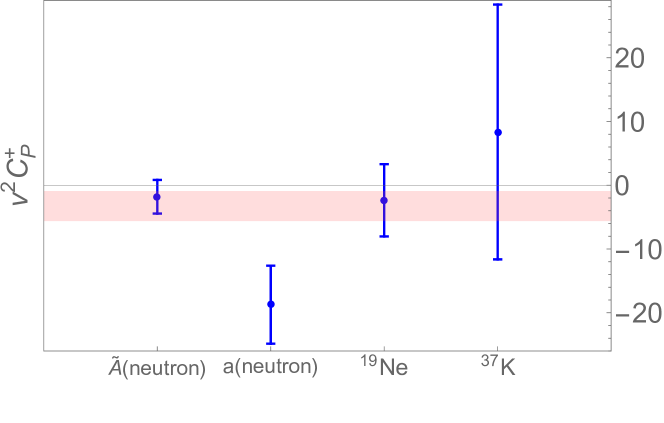
Figure 1: Constraints on the pseudo-scalar coefficient $C_{P}^{+}$ from a subset of most sensitive observables. We show the fit to $C_{P}^{+}$ marginalized over $C_{V}^{+}$ and $C_{A}^{+}$, assuming other Wilson coefficients vanish. The error bars show the 68% CL intervals obtained using ${\cal F}t(0^{+}\to 0^{+})$, neutron’s lifetime, and one of the following: neutron’s beta asymmetry, neutron’s $\beta$-$\nu$ correlation, ${\cal F}t$ and beta asymmetry of ¹⁹Ne, or ${\cal F}t$, beta asymmetry, and neutrino asymmetry of ³⁷K. The pink band corresponds to the global fit in Eq. 33.

We can relax our assumptions by allowing new physics to enter also via scalar and tensor interactions at the quark level, which leads to $C_{S}^{+}$ and $C_{T}^{+}$ being non-zero in the leading order Lagrangian in Eq. 8. The existing experimental data allows for a simultaneous fit of all five Wilson coefficients:

$$v^{2}\begin{pmatrix}C_{V}^{+}\\ C_{A}^{+}\\ C_{S}^{+}\\ C_{T}^{+}\\ C_{P}^{+}\end{pmatrix}=\begin{pmatrix}\phantom{-}0.98544(49)\\ -1.25818(82)\\ -0.0005(12)\\ 0.0008(16)\\ -5.9(4.4)\end{pmatrix},\qquad\rho=\left(\begin{array}[]{ccccc}1&-0.07&0.85&0.22&0.45\\ \text{}&1&-0.06&-0.84&0.73\\ \text{}&\text{}&1&0.24&0.38\\ \text{}&\text{}&\text{}&1&-0.64\\ \text{}&\text{}&\text{}&\text{}&1\\ \end{array}\right).$$ (34)

Introduction of $C_{S}^{+}$ and $C_{T}^{+}$ increases the degeneracy of the parameter space, leading to the constraints on $C_{V}^{+}$, $C_{A}^{+}$ and $C_{P}^{+}$ being relaxed by approximately a factor of two compared to the simplified scenario in Eq. 33. This is enough to disentangle the five independent WEFT couplings present in Eq. (1). At linear order in new physics, they can be identified with the new physics parameters $\epsilon_{R,S,P,T}$ and the “polluted” CKM element corresponding to the combination $\hat{V}_{ud}\equiv V_{ud}(1+\epsilon_{L}+\epsilon_{R})$ Falkowski:2020pma . Indeed, using the matching in Sections 2.3 and 2.3, we can translate the fit above into constraints on the parameters of the quark-level Lagrangian in Eq. 1, in such a way that all the new physics parameters except for $\epsilon_{L}$ can be disentangled. We obtain

$$\begin{pmatrix}\hat{V}_{ud}\\ \epsilon_{S}\\ \epsilon_{T}\\ \epsilon_{R}\\ \epsilon_{P}\end{pmatrix}=\begin{pmatrix}0.97353(49)\\ -0.0004(12)\\ 0.0008(17)\\ -0.010(11)\\ -0.017(13)\end{pmatrix},\qquad\rho=\left(\begin{array}[]{ccccc}1&0.83&0.21&0.02&0.44\\ \text{}&1&0.24&0.02&0.38\\ \text{}&\text{}&1&-0.02&-0.64\\ \text{}&\text{}&\text{}&1&0.03\\ \text{}&\text{}&\text{}&\text{}&1\\ \end{array}\right).$$ (35)

This is the first time such general constraints, including those on the pseudoscalar parameter $\epsilon_{P}$, are extracted from nuclear data. Inclusion of $\epsilon_{P}$ in the fit does not increase substantially the uncertainty on the remaining new physics parameters (see the fit without $\epsilon_{P}$ in Ref. Falkowski:2020pma ), as also indicated by moderate off-diagonal entries in the last row/column of the correlation matrix. Curiously, the uncertainty on $\epsilon_{P}$ is only percent-level, which is even slightly smaller than that on $\epsilon_{R}$. The lower sensitivity to the latter is in part a consequence of the relatively large uncertainty of the lattice input for $g_{A}$ when we match to Section 2.3, but it also shows that beta transitions have decent sensitivity to pseudocalar interactions, even though their effects are suppressed by $\mathcal{O}(m_{e}/m_{N})\sim 10^{-3}$, thanks to the large value of the pseudoscalar charge $g_{P}$ Gonzalez-Alonso:2013ura . All in all, the magnitudes of $\epsilon_{X}$ effectively probed by beta transitions is well within the validity range of the quark-level EFT. However, the sensitivity of beta transitions to $\epsilon_{P}$ is well inferior to that of pion decays. Very recently, Ref. Cirigliano:2021yto obtained the constraint $\epsilon_{P}=3.9(4.3)\times 10^{-6}$ in the combined fit to beta and pion decay data. This is more than three orders of magnitude better than the result in Eq. 35 based nuclear beta transitions alone.

4.2 Weak magnetism

The name weak magnetism refers to a sum of two distinct effects entering at the subleading order in recoil. One is the contribution to the decay amplitude due to the operator

$$\mathcal{L}^{(1)}\supset-C_{M}^{+}{1\over 2m_{N}}\epsilon^{ijk}(\psi_{p}^{\dagger}\sigma^{j}\psi_{n})\nabla_{i}\big{(}\bar{e}_{L}\gamma^{k}\nu_{L}\big{)}$$ (36)

in the subleading EFT Lagrangian in Section 2.3. We will refer to this effect as the universal weak magnetism, because it is common for all nuclear transitions. It turns out that a part of the contribution of another operator in Section 2.3,

$$\mathcal{L}^{(1)}\supset-C^{+}_{FV}{i\over 2m_{N}}(\psi_{p}^{\dagger}\overleftrightarrow{\nabla}_{k}\psi_{n})(\bar{e}_{L}\gamma^{k}\nu_{L}),$$ (37)

has the same tensor structure as that originating from Eq. 36. Namely, using the parametrization of the $\langle\psi_{p}^{\dagger}\overleftrightarrow{\nabla}_{k}\psi_{n}\rangle$ matrix element in Section 3.1 and retaining only the part proportional to $\beta_{FV}$, the subleading decay amplitude is affected by the operators in Eq. 36 and Eq. 37 as

$${\mathcal{M}}_{\beta^{-}}^{(1)}\supset i\big{(}C_{M}^{+}+\beta_{FV}C^{+}_{FV}\big{)}rM_{F}A\epsilon^{ijk}\bm{q}^{i}{[{\cal T}_{(J)}^{j}]_{J_{z}^{\prime}J_{z}}\over\sqrt{J(J+1)}}L^{k}.$$ (38)

We will refer to the contribution entering via the operator in Eq. 37 as the nucleus-dependent contribution to weak-magnetism (because the form factor $\beta_{FV}$ depends on the nuclei participating in the transition) or, in short, nuclear weak magnetism. Once again, it is instructive to first display the correlations in a simplified setting where we only take into account the interference between weak magnetism and the leading SM effects proportional to $C_{V}^{+}$ and $C_{A}^{+}$. Defining $C^{+}_{WM}\equiv C_{M}^{+}+\beta_{FV}C^{+}_{FV}$, at the linear order in recoil the total (universal+nuclear) weak magnetism enters the relevant correlations as:

$$\xi_{b}(E_{e})= \pm r^{2}{2(E_{e}^{\rm max}-2E_{e}+m_{e}^{2}/E_{e})\over 3m_{N}}{C_{A}^{+}C^{+}_{WM}\over(C_{V}^{+})^{2}+r^{2}(C_{A}^{+})^{2}},$$

$$\Delta a(E_{e})= \pm r^{2}{2(2E_{e}-E_{e}^{\rm max})\over 3m_{N}}{C_{A}^{+}C^{+}_{WM}\over(C_{V}^{+})^{2}+r^{2}(C_{A}^{+})^{2}},$$

$$\Delta A(E_{e})= \mp r\sqrt{J\over J+1}{2(E_{e}^{\rm max}-E_{e})\over 3m_{N}}{C_{V}^{+}C^{+}_{WM}\over(C_{V}^{+})^{2}+r^{2}(C_{A}^{+})^{2}}+{r^{2}\over J+1}{5E_{e}-2E_{e}^{\rm max}\over 3m_{N}}{C_{A}^{+}C^{+}_{WM}\over(C_{V}^{+})^{2}+r^{2}(C_{A}^{+})^{2}},$$

$$\Delta B(E_{e})= \pm r\sqrt{J\over J+1}{2p_{e}^{2}\over 3m_{N}E_{e}}{C_{V}^{+}C^{+}_{WM}\over(C_{V}^{+})^{2}+r^{2}(C_{A}^{+})^{2}}+{r^{2}\over J+1}{3E_{e}E_{e}^{\rm max}-5E_{e}^{2}+2m_{e}^{2}\over 3m_{N}E_{e}}{C_{A}^{+}C^{+}_{WM}\over(C_{V}^{+})^{2}+r^{2}(C_{A}^{+})^{2}}.$$ (39)

See Section B.2 for the complete expressions including the interference with scalar and tensor currents and for the remaining correlations. Much as the pseudoscalar interactions in the previous subsections, weak magnetism is zero for pure Fermi transitions, in particular it does not affect the superallowed $0^{+}\to 0^{+}$ transitions. Unlike pseudoscalar, weak magnetism leads to all correlation coefficients picking up a dependence on the beta particle energy $E_{e}$.

	$n$	17F	19Ne	21Na	29P	35Ar	37K
$\langle\xi_{b}(E_{e})\rangle$	-0.1	-0.1	-0.1	-0.1	0.0	0.0	-0.1
$\langle\Delta a(E_{e})\rangle_{p}$	-1.8	1.1	1.2	0.5	0.3	0.1	0.3
$\langle\Delta A(E_{e})\rangle_{p}$	-3.1	1.3	-4.6	2.0	1.7	2.7	-6.1
$\langle\Delta B(E_{e})\rangle$	-0.3	-2.8	0.2	-3.5	-3.8	-3.3	4.5

Table 2: Sensitivity of the correlation coefficients in neutron and mirror decays to the nucleon-level weak magnetism parametrized by the Wilson coefficient $C_{M}^{+}$. The entries are in units of $10^{-4}$ and correspond to the averaged function multiplying $C_{M}^{+}$ in Section 4.2 for different parent nuclei. For the sake of this table, $C_{V}^{+}$, $C_{A}^{+}$, and $r$ are set to their minimum values in the SM fit (although they are kept as free parameters in the fits of this section). The averages $\langle\cdot\rangle_{(p)}$ over the $\beta$ particle energy $E_{e}$ are defined in Eqs. 25 and 29.

As discussed in Section 2, the numerical value of $C_{WM}^{+}$ for each transition is fixed by isospin symmetry (CVC), assuming the absence of large contributions to $C_{M}^{+}$ from higher-dimensional operators in the quark-level Lagrangian. More precisely, $C_{WM}^{+,\rm CVC}\approx(g_{M}^{\rm CVC}+\beta_{FV}^{\rm CVC})C_{V}^{+}$ up to small isospin breaking effects, where $g_{M}^{\rm CVC}=(\mu_{p}-\mu_{n})/\mu_{N}\approx 4.7$, and $\beta_{FV}^{\rm CVC}$ is transition-dependent and can be related to nuclear magnetic moments via Eq. 16. The goal of this subsection is to show that the existing experimental data is powerful enough to pinpoint universal weak magnetism parametrized by $C_{M}^{+}$, without a theoretical input from isospin symmetry.

Notice first that $\beta_{FV}=0$ for the neutron decay. Therefore, restricting to the subset of data that includes only the $0^{+}\to 0^{+}$ transitions and the neutron decay, we can directly determine $C_{M}^{+}$ (treated as a free parameter) along with other Wilson coefficients in the EFT Lagrangian. In the restricted framework where only $C_{V}^{+}$, $C_{A}^{+}$, and $C_{M}^{+}$ are non-zero, we obtain the simultaneous constraint on the remaining three Wilson coefficients:

$$v^{2}\begin{pmatrix}C_{V}^{+}\\ C_{A}^{+}\\ C_{M}^{+}\end{pmatrix}=\begin{pmatrix}0.98563(26)\\ -1.25785(52)\\ 3.6(1.1)\end{pmatrix},\qquad\rho=\left(\begin{array}[]{ccc}1&0.13&0.47\\ \text{}&1&0.66\\ \text{}&\text{}&1\\ \end{array}\right).$$ (40)

The fit is dominated by the measurements of ${\cal F}t(0^{+}\to 0^{+})$ (which fixes $C_{V}^{+}$), neutron’s lifetime (which then fixes $C_{A}^{+}$), and the neutron’s beta asymmetry (which then fixes $C_{M}^{+}$). We observe that the result is consistent with the CVC prediction $C_{M}^{+,\rm CVC}\approx 4.6/v^{2}$, and that $C_{M}^{+}=0$ is excluded at more than 3 sigma. To our knowledge this is the first experimental evidence for the universal (nucleon-level) weak magnetism.

We can sharpen this evidence somewhat by including data from mirror transitions studied in Ref. Falkowski:2020pma . In those cases $\beta_{FV}$ is non-zero, therefore those transitions do not give us an unobstructed access to the $C_{M}^{+}$ Wilson coefficient. Ideally for this argument, $\beta_{FV}$ would be determined by first principle calculations, for example by the lattice. In absence of such, for the sake of the fits below we fix $\beta_{FV}$ from the CVC relation in Eq. 16. Following this procedure we obtain

$$v^{2}\begin{pmatrix}C_{V}^{+}\\ C_{A}^{+}\\ C_{M}^{+}\end{pmatrix}=\begin{pmatrix}\phantom{-}0.98570(24)\\ -1.25778(48)\\ 3.86(87)\end{pmatrix},\qquad\rho=\left(\begin{array}[]{ccc}1&0.02&0.36\\ \text{}&1&0.60\\ \text{}&\text{}&1\\ \end{array}\right),$$ (41)

where the uncertainty on $C_{M}^{+}$ is improved by $\sim 20\%$ and the experimental evidence for universal weak magnetism is strengthened above $4\sigma$. The relative sensitivity of various observables contributing to this result is visualized in Fig. 2. Admittedly, our assumption that $\beta_{FV}=\beta_{FV}^{\rm CVC}$ makes the above argument a bit circular. Note however that the constraining power of the mirror data is currently dominated by the ¹⁹Ne decay Rebeiro:2018lwo ; Combs:2020ttz . Indeed, discarding all other mirror data except for ¹⁹Ne leads to $C_{M}^{+}=3.86(90)$, a negligible difference compared to Eq. 41. Furthermore, this result is very weakly sensitive to the precise value of $\beta_{FV}({}^{19}{\rm Ne})$ used in the fit. Using a much weaker assumption, $\beta_{FV}({}^{19}{\rm Ne})=(1\pm 1)\beta_{FV}^{\rm CVC}({}^{19}{\rm Ne})$, where $\beta_{FV}^{\rm CVC}({}^{19}{\rm Ne})=1.5$, leads to $C_{M}^{+}=3.80(94)$, which is still $4\sigma$ away from zero. We conclude that the further evidence for fundamental weak magnetism provided by the mirror data is robust.

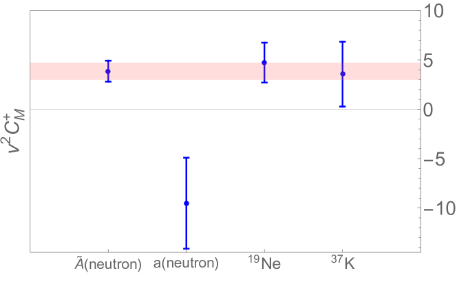
Figure 2: Constraints on the universal weak-magnetism $C_{M}^{+}$ from a subset of most sensitive observables. We show the fit to $C_{M}^{+}$ marginalized over $C_{V}^{+}$ and $C_{A}^{+}$, assuming other Wilson coefficients vanish. The error bars show the 68% CL intervals obtained using ${\cal F}t(0^{+}\to 0^{+})$, neutron’s lifetime, and one of the following: neutron’s beta asymmetry, neutron’s $\beta$-$\nu$ correlation, ${\cal F}t$ and beta asymmetry of ¹⁹Ne, or ${\cal F}t$, beta asymmetry, and neutrino asymmetry of ³⁷K. The pink band corresponds to the global fit in Eq. 41 and the dashed line marks the prediction of isospin symmetry.

Finally, we can also make a more general fit by allowing for new physics entering as scalar and tensor current at the leading order:

$$v^{2}\begin{pmatrix}C_{V}^{+}\\ C_{A}^{+}\\ C_{S}^{+}\\ C_{T}^{+}\\ C_{M}^{+}\end{pmatrix}=\begin{pmatrix}0.98576(44)\\ -1.2578(13)\\ 0.0002(11)\\ 0.0000(23)\\ 4.0(1.9)\end{pmatrix},\qquad\rho=\left(\begin{array}[]{ccccc}1&-0.41&0.83&0.53&-0.16\\ \text{}&1&-0.36&-0.93&0.91\\ \text{}&\text{}&1&0.5&-0.16\\ \text{}&\text{}&\text{}&1&-0.84\\ \text{}&\text{}&\text{}&\text{}&1\\ \end{array}\right).$$ (42)

Even in this more general framework the preference for non-zero $C_{M}^{+}$ is still at the $\sim 2\sigma$ level.

We remark that that all our fits in this section use only observables integrated over the energy spectrum of the beta particle, because only that information is provided by experimental collaborations in the readily usable form. On the other hand, as is clear from Section 4.2, weak magnetism predicts specific dependence of the correlations on $E_{e}$. Exploring this energy dependence will allow one to further tighten the theory-independent bounds on $C_{M}^{+}$, possibly pushing the evidence for weak magnetism beyond the $5\sigma$ threshold.

4.3 Induced tensor

As the final example of application of our formalism, we present the fit to the Wilson coefficient parametrizing the so-called induced tensor interactions in the subleading EFT Lagrangian in Section 2.3:

$$\mathcal{L}^{(1)}\supset-C_{E}^{+}{i\over 2m_{N}}(\psi_{p}^{\dagger}\sigma^{k}\psi_{n})\nabla_{k}\big{(}\bar{e}_{L}\gamma^{0}\nu_{L}\big{)}-C_{E^{\prime}}^{+}{i\over 2m_{N}}(\psi_{p}^{\dagger}\sigma^{k}\psi_{n})\partial_{t}\big{(}\bar{e}_{L}\gamma^{k}\nu_{L}\big{)}.$$ (43)

As discussed in Section 2, the UV matching relations for these Wilson coefficients imply $C^{+}_{E}=C_{E^{\prime}}^{+}=-C_{A}^{+}g_{IT}/g_{A}$, thus in the following we set $C_{E^{\prime}}^{+}=C_{E}^{+}$ and assume $C_{E}^{+}$ is real. We expect the nucleon-level parameter $g_{IT}$ to be suppressed by small isospin breaking effects, hence $v^{2}|C_{E}^{+}|$ is $\mathcal{O}(10^{-2}-10^{-3})$. But, as in the preceding subsection, we can ask the question what does experiment tell about $C_{E}^{+}$ without any theoretical input from isospin symmetry. At the level of interference with $C_{V}^{+}$ and $C_{A}^{+}$, the operators in Eq. 43 affect the correlations as

$$\xi_{b}(E_{e})= \pm r^{2}{2E_{e}^{\rm max}+m_{e}^{2}/E_{e}\over 3m_{N}}{C_{A}^{+}C_{E}^{+}\over(C_{V}^{+})^{2}+r^{2}(C_{A}^{+})^{2}},$$

$$\Delta a(E_{e})= \mp r^{2}{2E_{e}^{\rm max}\over 3m_{N}}{C_{A}^{+}C_{E}^{+}\over(C_{V}^{+})^{2}+r^{2}(C_{A}^{+})^{2}},$$

$$\Delta A(E_{e})= \mp r\sqrt{J\over J+1}{2(E_{e}^{\rm max}-E_{e})\over 3m_{N}}{C_{V}^{+}C_{E}^{+}\over(C_{V}^{+})^{2}+r^{2}(C_{A}^{+})^{2}}-{r^{2}\over J+1}{2E_{e}^{\rm max}+E_{e}\over 3m_{N}}{C_{A}^{+}C_{E}^{+}\over(C_{V}^{+})^{2}+r^{2}(C_{A}^{+})^{2}},$$

$$\Delta B(E_{e})= \mp r\sqrt{J\over J+1}{2E_{e}+m_{e}^{2}/E_{e}\over 3m_{N}}{C_{V}^{+}C_{E}^{+}\over(C_{V}^{+})^{2}+r^{2}(C_{A}^{+})^{2}}$$

$$+ {r^{2}\over J+1}{3E_{e}^{\rm max}-E_{e}+m_{e}^{2}/E_{e}\over 3m_{N}}{C_{A}^{+}C_{E}^{+}\over(C_{V}^{+})^{2}+r^{2}(C_{A}^{+})^{2}}.$$ (44)

See Sections B.3 and B.4 for the complete expressions including the interference with scalar and tensor currents and for the remaining correlations. Note that, in principle, isospin breaking contributions to the $\langle\psi_{p}^{\dagger}\sigma^{k}\overleftrightarrow{\nabla}_{k}\psi_{n}\rangle$ matrix element in Section 3.1 would lead to additional transition-dependent contributions to the correlations with the same functional form as Section 4.3. In this analysis we assume that such contributions are absent.

	$n$	17F	19Ne	21Na	29P	35Ar	37K
$\langle\xi_{b}(E_{e})\rangle$	-6.9	8.4	11.5	5.9	5.7	2.3	8.1
$\Delta a(E_{e})$	5.2	-7.5	-10.7	-5.6	-5.5	-2.3	-7.9
$\langle\Delta A(E_{e})\rangle_{p}$	4.8	5.1	7.6	5.8	7.6	4.2	-1.1
$\langle\Delta B(E_{e})\rangle$	-6.6	0.3	-11.7	0.6	-1.5	2.1	-9.6

Table 3: Sensitivity of the correlation coefficients in neutron and mirror decays to the induced tensor interactions parametrized by the Wilson coefficients $C_{E^{\prime}}^{+}=C_{E}^{+}$. The entries are in units of $10^{-4}$ and correspond to the averaged function multiplying $C_{E}^{+}$ in Section 4.3 for different parent nuclei. For the sake of this table, $C_{V}^{+}$, $C_{A}^{+}$, and $r$ are set to their minimum values in the SM fit (although they are kept as free parameters in the fits of this section). The averages $\langle\cdot\rangle_{(p)}$ over the $\beta$ particle energy $E_{e}$ are defined in Eqs. 25 and 29; for $\Delta a(E_{e})$ the induced tensor contribution is independent of $E_{e}$.

Assuming that $C_{E}^{+}$ is the only free parameter in the fit in addition to the SM Wilson coefficients $C_{V}^{+}$ and $C_{A}^{+}$, we obtain

$$v^{2}\begin{pmatrix}C_{V}^{+}\\ C_{A}^{+}\\ C_{E}^{+}\end{pmatrix}=\begin{pmatrix}0.98566(23)\\ -1.25881(90)\\ 1.7(1.1)\end{pmatrix},\qquad\rho=\left(\begin{array}[]{ccc}1&0.16&-0.30\\ \text{}&1&-0.90\\ \text{}&\text{}&1\\ \end{array}\right).$$ (45)

Clearly, the existing data are sensitive only to $|C_{E}^{+}|\sim 1/v^{2}$ (similarly as for the other recoil-level Wilson coefficients, e.g. $C_{P}^{+}$ or $C_{M}^{+}$). This is 3 orders of magnitude larger than the theoretically expected magnitude and hence experimental detection of $C_{E}^{+}$ is unlikely in the envisagable future. Furthermore, the current data show a mild $~{}1.6\sigma$ preference for a non-zero $C_{E}^{+}$, driven largely by the measurement of neutron’s $\beta$-$\nu$ correlation in the aSPECT experiment Beck:2019xye . It will be interesting to see if this preference goes away, as experiments acquire more precise data.

5 Conclusions

In this paper we discussed the EFT for beta transitions. Working in the framework of the pionless EFT, with nucleons as degrees of freedom, the effective interactions between nucleons and leptons were organized in a non-relativistic expansion in powers of $\bm{\nabla}/m_{N}$. The novelty of this paper is that the low-energy EFT was matched to the general quark-level EFT at higher energy. The latter, which we refer to as the WEFT, describes the effects of the SM weak interactions, as well as possible effects of new heavy particles from beyond the SM. We worked out the matching between the WEFT and the low-energy EFT up to the subleading order in $\bm{\nabla}/m_{N}$, that is including the linear recoil effects. The results in Section 2.3 and Section 2.3 describe the matching conditions for the Wilson coefficients of the leading and subleading Lagrangian in Eq. 8 and Section 2.3. In particular, the matching of the non-standard tensor interactions in the WEFT to the recoil-level non-relativistic interactions at low energy was worked out for the first time.

The EFT framework allows us to systematically describe how the standard and non-standard weak interactions affect beta decay observables, such as the lifetime, beta energy spectrum, and various angular correlations. We calculated the impact of all the terms in the leading and subleading Lagrangian on the differential decay width in allowed beta transitions summed over the beta particle and daughter nucleus polarizations. In Sections 3.2 and B.10 we list all correlation coefficients that appear at the leading and subleading orders in recoil; the ones in Section B.10 receive recoil-level contributions only in the presence of tensor interactions. We express the correlation coefficients in terms of the Wilson coefficients of the effective Lagrangian and matrix elements of non-relativistic nucleon currents. Partial results, most relevant for our numerical analysis, were displayed in Section 4, while the complete results are collected in Appendix B.

With the expressions for the observables at hand, we can use the existing experimental data on beta transitions to determine confidence intervals for the Wilson coefficients in the EFT Lagrangian. For the leading Lagrangian this exercise was already completed in Ref. Falkowski:2020pma , where $\mathcal{O}(10^{-4})$ relative precision was found for the standard Wilson coefficients corresponding to the vector and axial currents, and stringent constraints were established on the non-standard scalar and tensor interactions. In this paper we extended this analysis to recoil-level Wilson coefficients. In particular, we performed the first ever comprehensive analysis of the pseudoscalar interactions in allowed beta decay. We find that nuclear decays set a robust constraint on the Wilson coefficient descending from the pseudoscalar interactions in the WEFT, even though it enters the observables only at the linear order in recoil. This translates into a percent-level constraint on the pseudoscalar WEFT parameter ($\epsilon_{P}$ in Eq. 1), which is comparable to the sensitivity to the right-handed WEFT current ($\epsilon_{R}$), and one order of magnitude weaker than the sensitivity to the scalar and tensor currents ($\epsilon_{S}$ and $\epsilon_{T}$). One should note, however, that within the WEFT framework, constraints on $\epsilon_{P}$ from pion decays are 4 orders of magnitude stronger. It would be interesting to extend this analysis to the recoil-level effects of tensor interactions. In particular, at this order, tensor interactions contribute to the very precisely measured $0^{+}\to 0^{+}$ transitions. However, a quantitative analysis of this kind would require (at least approximate) knowledge of the subleading tensor charges $g_{T}^{(1,3)}$, cf. Section 2.2, as well as of the nuclear form factors $\alpha_{FT}$ and $\gamma_{FT}$, cf. Section 3.1.

Weak magnetism is another recoil-level effect to which experiment is sensitive. Our global analysis of the allowed beta decay data showed a 3 sigma evidence for a non-zero value of the EFT Wilson coefficient corresponding to the universal (nucleon-level) weak magnetism. The evidence is dominated by the neutron decay measurements (lifetime and beta asymmetry), and is further strengthened by mirror decay data. We also discussed the recoil-level EFT operator describing the so-called induced tensor interactions. The isospin symmetry of QCD predicts that this Wilson coefficient should be suppressed so as to give negligible contributions to observables. Instead, our global analysis showed a small $1.8~{}\sigma$ preference for non-zero induced tensor interactions. Future measurements and better theoretical calculations will improve the understanding of the effects of these Wilson coefficients.

Appendix A Symmetry constraints on nuclear matrix elements

In this appendix we discuss the nuclear matrix elements of the form

$$\bra{{\cal N^{\prime}}}\bar{p}\Gamma n\ket{{\cal N}}.$$ (46)

Here, $\ket{\cal N}$ and $\ket{\cal N^{\prime}}$ are nuclear states with spin $J$, $J_{z}$ and $J_{z}^{\prime}$ projection of the spin on the z-axis, and momenta $p$ and $p^{\prime}$. They both belong to the same isospin multiplet with the isospin quantum number $j$ and the isospin projections related by $j_{3}^{\prime}-j_{3}=1$. The operator sandwiched between the states is made of relativistic neutron and proton fields $n$ and $p$ evaluated at $x=0$. Below we will consider the vector, axial, and tensor matrix elements, that is $\Gamma=\gamma^{\mu},\gamma^{\mu}\gamma^{5},\sigma^{\mu\nu}$. We do not consider the (pseudo)scalar cases because, as we will see, they are not needed to extract the non-relativistic matrix elements that we are interested in.

The aim of this appendix is to write down the most general expression for the matrix element in Eq. 46 consistent with Lorentz invariance and the discrete symmetries of the strong interactions: parity and time reversal invariance. We will work in the isospin limit where ${\cal N}$ and ${\cal N^{\prime}}$ (and also $p$ and $n$) have the same mass, thus $p^{2}=p^{\prime}{}^{2}=m_{\cal N}^{2}$. In this limit, the matrix element is also invariant under another discrete symmetry called G-parity, which can be defined as a product of $P$, $T$, and a 180 degrees isospin rotation. Given the relativistic matrix elements, it will be straightforward to take the non-relativistic limit where $\bm{p}$ and $\bm{p}^{\prime}$ are much smaller than the nucleon mass, and by this means to determine the most general form of the non-relativistic matrix elements used in our analysis.

A.1 Spin-J representation matrices

We first introduce the spin-J representation matrices ${\cal T}_{(J)}^{k}$, which appear in nuclear matrix elements at the leading and subleading order of recoil expansion. It is convenient to define them in terms of the Clebsch-Gordan coefficients. The latter are denoted by $C(J_{1},m_{1};J_{2},m_{2};J,m)$ and defined by $\ket{J,m}=\sum_{m_{i}=-J_{i}}^{J_{i}}C(J_{1},m_{1};J_{2},m_{2};J,m)\ket{J_{1},m_{1}}\otimes\ket{J_{2},m_{2}}$ with the Condon–Shortley phase conventions. We can define the $(2J+1)\times(2J+1)$-dimensional matrices ${\cal T}_{(J)}^{k}$ as follows

$$\,[{\cal T}_{(J)}^{1}]^{\,J_{z}}_{J_{z}^{\prime}}\equiv -\sqrt{J(J+1)\over 2}\bigg{[}C(J,J_{z};1,1;J,J_{z}^{\prime})-C(J,J_{z};1,-1;J,J_{z}^{\prime})\bigg{]},$$

$$\,[{\cal T}_{(J)}^{2}]^{\,J_{z}}_{J_{z}^{\prime}}\equiv \,i\,\sqrt{J(J+1)\over 2}\bigg{[}C(J,J_{z};1,1;J,J_{z}^{\prime})+C(J,J_{z};1,-1;J,J_{z}^{\prime})\bigg{]},$$

$$\,[{\cal T}_{(J)}^{3}]^{\,J_{z}}_{J_{z}^{\prime}}\equiv \,\sqrt{J(J+1)}\,C(J,J_{z};1,0;J,J_{z}^{\prime}).$$ (47)

These are the familiar spin-J generators of the $SO(3)$ Lie algebra, normalized such that ${\cal T}_{(J)}^{3}={\rm diag}(J,J-1,\dots,-J)$. In particular ${\cal T}_{(0)}^{k}=0$, ${\cal T}_{(1/2)}^{k}=\sigma^{k}/2$, and

$${\cal T}_{(1)}^{1}=\left(\begin{array}[]{ccc}0&\frac{1}{\sqrt{2}}&0\\ \frac{1}{\sqrt{2}}&0&\frac{1}{\sqrt{2}}\\ 0&\frac{1}{\sqrt{2}}&0\\ \end{array}\right),\quad{\cal T}_{(1)}^{2}=\left(\begin{array}[]{ccc}0&-\frac{i}{\sqrt{2}}&0\\ \frac{i}{\sqrt{2}}&0&-\frac{i}{\sqrt{2}}\\ 0&\frac{i}{\sqrt{2}}&0\\ \end{array}\right),\quad{\cal T}_{(1)}^{3}=\left(\begin{array}[]{ccc}1&0&0\\ 0&0&0\\ 0&0&-1\\ \end{array}\right).$$ (48)

One property of the ${\cal T}_{(J)}^{1,2}$ matrices is that, for any $J$, the only non-zero entries are those with $|J_{z}-J_{z}^{\prime}|=1$. For $J\geq 1$ we can also define the 2-index Hermitian and traceless matrices:

$${\cal T}_{(J)}^{kl}\equiv{\cal T}_{(J)}^{k}{\cal T}_{(J)}^{l}+{\cal T}_{(J)}^{l}{\cal T}_{(J)}^{k}-{2\over 2J+1}\mathrm{T}\mathrm{r}[{\cal T}_{(J)}^{k}{\cal T}_{(J)}^{l}]\bm{1}_{2J+1}.$$ (49)

These can appear in nuclear matrix elements at the subleading order in recoil expansion, and have non-zero entries for $|J_{z}-J_{z}^{\prime}|\leq 2$. The matrices ${\cal T}_{(J)}^{k}$ and ${\cal T}_{(J)}^{kl}$ satisfy the useful sum rules (for any value of $J_{z}$):

$$\sum_{J_{z}^{\prime}=-J}^{J}[{\cal T}_{(J)}^{k}]^{\,J_{z}}_{J_{z}^{\prime}}\delta_{J_{z}^{\prime}J_{z}}= J^{k},$$

$$\sum_{J_{z}^{\prime}=-J}^{J}[{\cal T}_{(J)}^{k}]^{\,J_{z}}_{J_{z}^{\prime}}[{\cal T}_{(J)}^{l\,*}]^{\,J_{z}}_{J_{z}^{\prime}}= {J(J+1)\over 3}\delta^{kl}+{J(J+1)-3(\bm{J}\bm{j})^{2}\over 6}\big{(}\delta^{kl}-3j^{k}j^{l}\big{)}-{i\over 2}\epsilon^{klr}J^{r},$$

$$\sum_{J_{z}^{\prime}=-J}^{J}[{\cal T}_{(J)}^{kl}]^{\,J_{z}}_{J_{z}^{\prime}}\delta_{J_{z}^{\prime}J_{z}}= {J(J+1)-3(\bm{J}\bm{j})^{2}\over 3}\big{(}\delta^{kl}-3j^{k}j^{l}\big{)},$$

$$\sum_{J_{z}^{\prime}=-J}^{J}[{\cal T}_{(J)}^{kl}]^{\,J_{z}}_{J_{z}^{\prime}}[{\cal T}_{(J)}^{j\,*}]^{\,J_{z}}_{J_{z}^{\prime}}= {(2J+3)(2J-1)\over 6}\big{(}\delta^{jk}J^{l}+\delta^{jl}J^{k}\big{)}-J^{j}\big{(}4J^{k}J^{l}-j^{k}j^{l}\big{)}$$

$$+ {J(J+1)-3(\bm{J}\bm{j})^{2}\over 3}\bigg{[}\big{(}\delta^{kl}-3j^{k}j^{l}\big{)}J^{j}+\big{(}\delta^{kj}-3j^{k}j^{j}\big{)}J^{l}+\big{(}\delta^{lj}-3j^{j}j^{l}\big{)}J^{k}\bigg{]}$$

$$+ i{3\over 2}\bigg{[}\epsilon^{jkn}J^{l}+\epsilon^{jln}J^{k}\bigg{]}J^{n}-i{J(J+1)\over 2}\bigg{[}\epsilon^{jkn}j^{l}+\epsilon^{jln}j^{k}\bigg{]}j^{n}.$$ (50)

A.2 Spinor conventions

We will express relativistic nuclear matrix elements in terms of commuting spinor variables using the formalism introduced in Ref. Arkani-Hamed:2017jhn . Here we provide a lightning review of this formalism.

Let us first define our conventions for the 2-component spinor algebra. We work in four dimensions with the mostly-minus metric $\eta_{\mu\nu}={\rm diag}(1,-1,-1,-1)$. The Lorentz algebra can be decomposed into $SL(2,\mathbb{C})\times SL(2,\mathbb{C})$. Holomorphic and anti-holomorphic spinors $\chi_{\alpha}$ and $\tilde{\chi}_{\dot{\alpha}}$, $\alpha=1,2$, transform under the respective $SL(2,\mathbb{C})$ factors with indices being raised and lowered by the antisymmetric epsilon tensor:

$$\chi^{\alpha}=\epsilon^{\alpha\beta}\chi_{\beta}~{},\quad\chi_{\alpha}=\epsilon_{\alpha\beta}\chi^{\beta}~{},\qquad\tilde{\chi}^{\dot{\alpha}}=\epsilon^{\dot{\alpha}\dot{\beta}}\tilde{\chi}_{\dot{\beta}}~{},\quad\tilde{\chi}_{\dot{\alpha}}=\epsilon_{\dot{\alpha}\dot{\beta}}\tilde{\chi}^{\dot{\beta}}~{},$$ (51)

where summing over repeated spinor indices is implicit, and we use the convention $\epsilon^{12}=1$, $\epsilon_{12}=-1$. One can construct Lorentz invariants from two holomorphic or two anti-holomorphic spinors: $\chi\psi\equiv\chi^{\alpha}\psi_{\alpha}$, $\tilde{\chi}\tilde{\psi}\equiv\tilde{\chi}_{\dot{\alpha}}\tilde{\psi}^{\dot{\alpha}}$. Furthermore, spinor indices can be traded for the vector ones with the help of the sigma matrices: $[\sigma^{\mu}]_{\alpha\dot{\beta}}=(\mathbb{I},\bm{\sigma})$ and $[\bar{\sigma}^{\mu}]^{\dot{\alpha}\beta}=(\mathbb{I},-\bm{\sigma})$, where $\bm{\sigma}$ are the usual Pauli matrices. For example, $\chi\sigma^{\mu}\tilde{\psi}\equiv\chi^{\alpha}[\sigma^{\mu}]_{\alpha\dot{\beta}}\tilde{\psi}^{\dot{\beta}}$ and $\tilde{\chi}\bar{\sigma}^{\mu}\psi\equiv\tilde{\chi}_{\dot{\alpha}}[\bar{\sigma}^{\mu}]^{\dot{\alpha}\beta}\psi_{\beta}$ both transform as Lorentz vectors. In the 2-component context we also define $\sigma^{\mu\nu}\equiv{i\over 2}(\sigma^{\mu}\bar{\sigma}^{\nu}-\sigma^{\nu}\bar{\sigma}^{\mu})$ and $\bar{\sigma}^{\mu\nu}\equiv{i\over 2}(\bar{\sigma}^{\mu}\sigma^{\nu}-\bar{\sigma}^{\nu}\sigma^{\mu})$, using which one can construct Lorentz tensors $\chi\sigma^{\mu\nu}\psi$ and $\tilde{\chi}\bar{\sigma}^{\mu\nu}\tilde{\psi}$.

Consider now a massive particle whose (four-)momentum $p$ satisfies the on-shell condition $p^{2}=m^{2}$. We treat $p$ as incoming momentum, thus $p^{0}>0$ for initial state particles, and $p^{0}<0$ for final state particles. The momentum can be equivalently represented by four commuting two-component spinors $\chi^{K}$ and $\tilde{\chi}_{K}$, where $K=1,2$:

$$[p_{\mu}\sigma^{\mu}]_{\alpha\dot{\beta}}=\sum_{K=1}^{2}\chi_{\alpha}^{\,K}\tilde{\chi}_{\dot{\beta}\,K}~{},\qquad(p\bar{\sigma})^{\alpha\dot{\beta}}=\sum_{K=1}^{2}\tilde{\chi}^{\dot{\alpha}}_{\,K}\chi^{\beta\,K}\,.$$ (52)

In our conventions the spinors are normalized as

$$(\chi^{K}\chi_{L})=\delta^{K}_{L}m~{},\qquad(\tilde{\chi}_{K}\tilde{\chi}^{L})=\delta_{K}^{L}m~{}.$$ (53)

It follows that they satisfy the Dirac equation:

$$(p_{\mu}\sigma^{\mu})\tilde{\chi}^{K}=m\chi^{K}~{},\quad(p_{\mu}\bar{\sigma}^{\mu})\chi^{K}=m\tilde{\chi}^{K}~{},\quad\chi^{K}(p_{\mu}\sigma^{\mu})=-m\tilde{\chi}^{K}~{},\quad\tilde{\chi}^{K}(p_{\mu}\bar{\sigma}^{\mu})=-m\chi^{K}~{}.$$ (54)

Eqs. 52 and 53 are invariant under the $SU(2)$ little group rotation of the spinors: $\chi^{K}\to[U]^{K}_{\,L}\chi^{L}$, $\chi_{K}\to\chi_{L}[U^{\dagger}]^{L}_{\,K}$, $\chi_{K}\to[U^{*}]_{K}^{\,L}\chi_{L}$. where from now on summation over repeated little group indices is implicit. In complete analogy to spinor indices, the little group indices can be raised and lowered by the epsilon tensor: $\chi_{K}=\epsilon_{KL}\chi^{L}$, etc. For a real momentum $p$ the spinors $\chi$ and $\tilde{\chi}$ are related by complex conjugation. For an initial-state particle (positive $p^{0}$) we have

$$(\chi_{\alpha}^{\,K})^{*}=\tilde{\chi}_{\dot{\alpha}\,K}~{},\quad(\tilde{\chi}_{\dot{\alpha}\,K})^{*}=\chi_{\alpha}^{\,K}~{},\quad(\tilde{\chi}_{\dot{\alpha}}^{\,K})^{*}=-\chi_{\alpha\,K}~{},\quad(\chi_{\alpha\,K})^{*}=-\tilde{\chi}_{\dot{\alpha}}^{\,K}~{},$$ (55)

while for a final-state particle (negative $p^{0}$) the signs on the right-hand sides of Eq. 55 are reversed.

Let us parametrize particle’s 3-momentum as $\bm{p}=|p|\bm{n}$, where $\bm{n}\equiv(\sin\theta\cos\phi,\sin\theta\sin\phi,\cos\theta)$ is the unit 3-vector in the direction of motion. A convenient representation of the corresponding spinors is

$$\chi^{K}= {\sqrt{E_{p}+|p|}+\sqrt{E_{p}-|p|}\over 2}\eta^{K}+{\sqrt{E_{p}+|p|}-\sqrt{E_{p}-|p|}\over 2}\zeta^{K}~{},$$

$$\tilde{\chi}^{K}= \pm{\sqrt{E_{p}+|p|}+\sqrt{E_{p}-|p|}\over 2}\tilde{\eta}^{K}\pm{\sqrt{E_{p}+|p|}-\sqrt{E_{p}-|p|}\over 2}\tilde{\zeta}^{K}~{},$$ (56)

where $E_{p}=\sqrt{|p|^{2}+m^{2}}$, the upper (lower) sign refers to an initial- (final-) state particle, and we introduced

$$\eta_{\alpha}^{K}\equiv \delta_{\alpha}^{K}~{},\qquad\zeta_{\alpha}^{K=1}\equiv\begin{pmatrix}-\cos\theta\\ -e^{i\phi}\sin\theta\end{pmatrix}~{},\quad\zeta_{\alpha}^{K=2}\equiv\begin{pmatrix}-e^{-i\phi}\sin\theta\\ \cos\theta\end{pmatrix}~{}.$$ (57)

The representation of Section A.2 is particularly useful in the non-relativistic limit, because the small-velocity expansion is the same as the expansion in powers of $\zeta$’s.

Lorentz invariance implies that an amplitude describing scattering of $n$ massive particles with spins $J_{i}$, $i=1\dots n$ must be a scalar function of the relevant momenta $p_{i}^{\mu}$ and spinors $\chi_{i}$, $\tilde{\chi}_{i}$. Moreover, little group covariance requires that the amplitude contains exactly $2J_{i}$ of the spinors $\chi_{i}$ or $\tilde{\chi}_{i}$ with uncontracted little group indices (spinors with contracted little group indices can be traded for momenta using Eq. 52). Initial-state particles will be represented by spinors with raised little group indices, $\chi_{i}^{K_{j}}$ or $\tilde{\chi}_{i}^{K_{j}}$, $j=1\dots 2J_{i}$, while final-state particles will be represented by spinors with lowered little group indices, $\chi_{i\,L_{j}}$, $\tilde{\chi}_{i\,L_{j}}$. The little group indices corresponding to the same particle are always implicitly symmetrized. To reduce clutter, the little group indices are often omitted whenever it does not lead to ambiguities.

In the representation of Section A.2, the little group index of a spinor or a twiddle spinor corresponds to the projection of particle’s polarization $J_{z}$ on the z-axis. For example, an initial-state spin 1/2 particle with polarization $J_{z}=+1/2$ is represented by $\chi^{K=1}$, and $J_{z}=-1/2$ is represented by $\chi^{K=2}$. Likewise, for a final-state particle we use $\chi_{L=1}$ for $J_{z}=+1/2$, and $\chi_{L=2}$ for $J_{z}=-1/2$. For an initial-state spin-1, a pair ($\chi^{K=1}$, $\chi^{K=1}$) represents $J_{z}=+1$, a pair ($\chi^{K=1}$, $\chi^{K=2}$) represents $J_{z}=0$ (after symmetrizing the little group index), and ($\chi^{K=2}$, $\chi^{K=2}$) represents $J_{z}=-1$. And so on. Other spin quantization axes can be obtained from Section A.2 by appropriate little group rotations, e.g. the helicity representation is obtained using the SU(2) rotation matrix $U=\begin{pmatrix}\cos{\theta\over 2}&e^{i\phi}\sin{\theta\over 2}\\ -e^{-i\phi}\sin{\theta\over 2}&\cos{\theta\over 2}\end{pmatrix}$.

A.3 Discrete symmetries

The spinor formalism allows for a transparent description of the discrete symmetries corresponding to the parity ($\bm{x}\to-\bm{x}$) and time reversal ($t\to-t$) invariance of the strong interactions. The matrix element in Eq. 46 can be expressed as a functional $F$ of the momenta $p^{\mu}$, $p^{\prime}{}^{\mu}$ and of the spinor variables $\chi_{1}$, $\chi_{2}$ associated with these momenta. Parity and time reversal invariance can be re-formulated as constraints on the functional $F$. In the discussion below, we will always assume that ${\cal N}$ and ${\cal N}^{\prime}$ transform in the same way under parity and time reversal (in particular, they are both parity-even, or both parity-odd).

The relevant nucleon bi-linears transform under the unitary Hilbert space parity operator ${\cal P}$ as ${\cal P}[\bar{p}\Gamma n(t,\bm{x})]{\cal P}^{-1}=\eta_{\Gamma}^{P}\bar{p}\Gamma n(t,-\bm{x})$, where the values of $\eta_{\Gamma}^{P}$ are collected in Table 4. Then, parity conservation implies that $F\stackrel{{\scriptstyle P}}{{\to}}\eta_{\Gamma}^{P}F$ under the following transformation $P$ of the spinors and momenta:

$$\chi_{1\,\alpha}\stackrel{{\scriptstyle P}}{{\leftrightarrow}} \tilde{\chi}_{1}^{\dot{\alpha}},\qquad\chi_{1}^{\alpha}\stackrel{{\scriptstyle P}}{{\leftrightarrow}}-\tilde{\chi}_{1\,\dot{\alpha}},\qquad\chi_{2\,\alpha}\stackrel{{\scriptstyle P}}{{\leftrightarrow}}-\tilde{\chi}^{\dot{\alpha}}_{2},\qquad\chi_{2}^{\alpha}\stackrel{{\scriptstyle P}}{{\leftrightarrow}}\tilde{\chi}_{2\,\dot{\alpha}},$$

$$P^{\mu}\stackrel{{\scriptstyle P}}{{\to}} (-)^{\mu}P^{\mu},\qquad q^{\mu}\stackrel{{\scriptstyle P}}{{\to}}(-)^{\mu}q^{\mu},$$ (58)

where $P^{\mu}=p^{\mu}+p^{\prime}{}^{\mu}$, $q^{\mu}=p^{\mu}-p^{\prime}{}^{\mu}$, $(-)^{\mu=0}\equiv 1$, $(-)^{\mu=1,2,3}\equiv-1$, and the sign difference between $\chi_{1}$ and $\chi_{2}$ transformations is due to the former (latter) corresponding to an initial-(final-) state particle. Little group indices are not displayed in Section A.3, but implicitly they always match, that is $\chi^{K}\stackrel{{\scriptstyle P}}{{\leftrightarrow}}\tilde{\chi}^{K}$, and $\chi_{K}\stackrel{{\scriptstyle P}}{{\leftrightarrow}}\tilde{\chi}_{K}$. It follows for example that $\chi_{1}\chi_{2}\pm\tilde{\chi}_{1}\tilde{\chi}_{2}$ transforms under $P$ into $\pm$ itself, while $\chi_{1}\sigma^{\mu}\tilde{\chi}_{2}\stackrel{{\scriptstyle P}}{{\to}}(-)^{\mu}\chi_{2}\sigma^{\mu}\tilde{\chi}_{1}$.

	$\bar{p}\gamma^{\mu}n$	$\bar{p}\gamma^{\mu}\gamma_{5}n$	$\bar{p}\sigma^{\mu\nu}n$
$\eta_{\Gamma}^{P}$	$(-)^{\mu}$	$-(-)^{\mu}$	$(-)^{\mu}(-1)^{\nu}$
$\eta_{\Gamma}^{T}$	$(-)^{\mu}$	$(-)^{\mu}$	$-(-)^{\mu}(-)^{\nu}$
$\eta_{\Gamma}^{PT}$	+1	-1	-1

Table 4: Transformation properties of the nucleon currents under parity and time reversal. We define $(-)^{\mu=0}\equiv 1$ and $(-)^{\mu=1,2,3}\equiv-1$.

For the anti-unitary Hilbert space time-reversal operator ${\cal T}$, the action on the nucleon bi-linears is ${\cal T}[\bar{p}\Gamma n(t,\bm{x})]{\cal T}^{-1}=\eta_{\Gamma}^{T}\bar{p}\Gamma n(-t,\bm{x})$, see Table 4. Time reversal implies that $F\stackrel{{\scriptstyle T}}{{\to}}\eta_{\Gamma}^{T}F^{*}$ under the following transformation $T$ of the spinors and momenta:

$$\chi_{i\,\alpha}\stackrel{{\scriptstyle T}}{{\to}} [\chi_{i}^{\alpha}]^{*},\quad\chi_{i}^{\alpha}\stackrel{{\scriptstyle T}}{{\to}}-[\chi_{i\,\alpha}]^{*},\qquad\tilde{\chi}_{i\,\dot{\alpha}}\stackrel{{\scriptstyle T}}{{\to}}[\tilde{\chi}_{i}^{\dot{\alpha}}]^{*},\quad\tilde{\chi}_{i}^{\dot{\alpha}}\stackrel{{\scriptstyle T}}{{\to}}-[\tilde{\chi}_{i\,\dot{\alpha}}]^{*},$$

$$P^{\mu}\stackrel{{\scriptstyle T}}{{\to}} (-)^{\mu}P^{\mu},\qquad q^{\mu}\stackrel{{\scriptstyle T}}{{\to}}(-)^{\mu}q^{\mu},$$ (59)

for $i=1,2$, and again the matching little group indices are implicit. It follows for example that both $[\chi_{1}\chi_{2}]^{*}$ and $[\tilde{\chi}_{1}\tilde{\chi}_{2}]^{*}$ transform into their complex conjugates under $T$, while $[\chi_{1}\sigma^{\mu}\tilde{\chi}_{2}]^{*}\stackrel{{\scriptstyle T}}{{\to}}(-)^{\mu}\chi_{1}\sigma^{\mu}\tilde{\chi}_{2}$.

Finally, we define $G$-parity as ${\cal G}=e^{i\pi\tau^{2}}{\cal T}{\cal P}$, where $e^{i\pi\tau^{2}}$ is the 180 degrees isospin rotation transforming $(p,n)\to(-n,p)$ and $({\cal N},{\cal N^{\prime}})\to(\mp{\cal N^{\prime}},\pm{\cal N})$. Isospin invariance implies that $F\stackrel{{\scriptstyle G}}{{\to}}\eta_{\Gamma}^{PT}F$ under the following transformation $G$ of the spinors and momenta:

$$\begin{pmatrix}\chi_{1}^{K}\\ \chi_{2\,L}\\ \tilde{\chi}_{1}^{K}\\ \tilde{\chi}_{2\,L}\end{pmatrix}\stackrel{{\scriptstyle G}}{{\to}}\begin{pmatrix}-\chi_{2\,L}\\ \chi_{1}^{K}\\ \tilde{\chi}_{2\,L}\\ -\tilde{\chi}_{1}^{K}\end{pmatrix},\qquad P^{\mu}\stackrel{{\scriptstyle G}}{{\to}}P^{\mu},\quad q^{\mu}\stackrel{{\scriptstyle G}}{{\to}}-q^{\mu}.$$ (60)

It follows for example that both $\chi_{1}\chi_{2}$ and $\tilde{\chi}_{1}\tilde{\chi}_{2}$ transform into itself under $G$, while $\chi_{1}\sigma^{\mu}\tilde{\chi}_{2}\stackrel{{\scriptstyle G}}{{\to}}\chi_{2}\sigma^{\mu}\tilde{\chi}_{1}$.

A.4 Relativistic matrix elements

Using the spinor formalism, the most general form of the relativistic nuclear matrix elements in Eq. 46 consistent with Lorentz, parity, time reversal, and G-parity invariance is

$$\bra{{\cal N^{\prime}}}\bar{p}\gamma^{\mu}n\ket{{\cal N}}= {\alpha_{V}\over(2m_{\cal N})^{2J}}\big{(}\chi_{1}\chi_{2}+\tilde{\chi}_{1}\tilde{\chi}_{2}\big{)}^{2J}P^{\mu}+{\beta_{V}\over(2m_{\cal N})^{2J-1}}\big{(}\chi_{1}\chi_{2}+\tilde{\chi}_{1}\tilde{\chi}_{2}\big{)}^{2J-1}\big{(}\chi_{1}\sigma^{\mu}\tilde{\chi}_{2}+\chi_{2}\sigma^{\mu}\tilde{\chi}_{1}\big{)}+\dots$$

$$\bra{{\cal N^{\prime}}}\bar{p}\gamma^{\mu}\gamma_{5}n\ket{{\cal N}}= {\beta_{A}\over(2m_{\cal N})^{2J-1}}\big{(}\chi_{1}\chi_{2}+\tilde{\chi}_{1}\tilde{\chi}_{2}\big{)}^{2J-1}\big{(}\chi_{1}\sigma^{\mu}\tilde{\chi}_{2}-\chi_{2}\sigma^{\mu}\tilde{\chi}_{1}\big{)}+\dots$$

$$\bra{{\cal N^{\prime}}}\bar{p}\sigma^{\mu\nu}n\ket{{\cal N}}= i{\alpha_{T}\over(2m_{\cal N})^{2J+1}}\big{(}\chi_{1}\chi_{2}+\tilde{\chi}_{1}\tilde{\chi}_{2}\big{)}^{2J}(P^{\mu}q^{\nu}-P^{\nu}q^{\mu})$$

$$+ {\beta_{T}\over(2m_{\cal N})^{2J-1}}\big{(}\chi_{1}\chi_{2}+\tilde{\chi}_{1}\tilde{\chi}_{2}\big{)}^{2J-1}\big{(}\chi_{1}\sigma^{\mu\nu}\chi_{2}+\tilde{\chi}_{1}\bar{\sigma}^{\mu\nu}\tilde{\chi}_{2}\big{)}$$

$$+ i{\gamma_{T}\over(2m_{\cal N})^{2J}}\big{(}\chi_{1}\chi_{2}+\tilde{\chi}_{1}\tilde{\chi}_{2}\big{)}^{2J-2}\big{(}\chi_{1}\chi_{2}-\tilde{\chi}_{1}\tilde{\chi}_{2}\big{)}\bigg{[}\big{(}\chi_{1}\sigma^{\mu}\tilde{\chi}_{2}-\chi_{2}\sigma^{\mu}\tilde{\chi}_{1}\big{)}P^{\nu}-(\mu\leftrightarrow\nu)\bigg{]}$$

$$+\dots$$ (61)

Above, the dots stand for terms leading to effects that are quadratic or higher order in recoil; e.g. in the axial matrix element we have $\big{(}\chi_{1}\chi_{2}+\tilde{\chi}_{1}\tilde{\chi}_{2}\big{)}^{2J-3}(\chi_{1}\chi_{2}-\tilde{\chi}_{1}\tilde{\chi}_{2}\big{)}^{2}\big{(}\chi_{1}\sigma^{\mu}\tilde{\chi}_{2}-\chi_{2}\sigma^{\mu}\tilde{\chi}_{1}\big{)}$, $\big{(}\chi_{1}\chi_{2}+\tilde{\chi}_{1}\tilde{\chi}_{2}\big{)}^{2J-5}(\chi_{1}\chi_{2}-\tilde{\chi}_{1}\tilde{\chi}_{2}\big{)}^{4}\big{(}\chi_{1}\sigma^{\mu}\tilde{\chi}_{2}-\chi_{2}\sigma^{\mu}\tilde{\chi}_{1}\big{)}$, and so on. Other similar terms in the axial matrix element, e.g. $\big{(}\chi_{1}\chi_{2}+\tilde{\chi}_{1}\tilde{\chi}_{2}\big{)}^{2J-2}(\chi_{1}\chi_{2}-\tilde{\chi}_{1}\tilde{\chi}_{2}\big{)}\big{(}\chi_{1}\sigma^{\mu}\tilde{\chi}_{2}-\chi_{2}\sigma^{\mu}\tilde{\chi}_{1}\big{)}$ or $\big{(}\chi_{1}\chi_{2}+\tilde{\chi}_{1}\tilde{\chi}_{2}\big{)}^{2J-1}\big{(}\chi_{1}\sigma^{\mu}\tilde{\chi}_{2}+\chi_{2}\sigma^{\mu}\tilde{\chi}_{1}\big{)}$ are forbidden by parity invariance. The form factors $\alpha_{V,T}$, $\beta_{V,A,T}$, $\gamma_{T}$ are in principle functions of $q^{2}$, but for our purpose they can be treated as constants. Time reversal invariance dictates that these form factors are all real. Eq. (61) is valid for any integer $2J\geq 0$ with the convention that whenever a naive evaluation of some term leads to spinors in a denominator then this term should be set to zero. In particular, for $J=0$ only the $\alpha_{V,T}$ structures survive, while for $J=1/2$ the $\gamma_{T}$ term should be set to zero.

As we discussed, Eq. 61 is obtained in the isospin limit, and in particular it does not contain G-parity-odd terms. These “second-class currents" in the nomenclature of Weinberg Weinberg:1958ut are often considered in the literature, and searched for in many experiments. For completeness, we list here the G-parity-odd contributions to the relativistic vector, axial, and tensor matrix elements that lead to effects of linear order in recoil:

$$\Delta\bra{{\cal N^{\prime}}}\bar{p}\gamma^{\mu}n\ket{{\cal N}}= {\alpha_{V}^{\prime}\over(2m_{\cal N})^{2J}}\big{(}\chi_{1}\chi_{2}+\tilde{\chi}_{1}\tilde{\chi}_{2}\big{)}^{2J}q^{\mu}$$

$$+ {\beta_{V}^{\prime}\over(2m_{\cal N})^{2J-1}}\big{(}\chi_{1}\chi_{2}+\tilde{\chi}_{1}\tilde{\chi}_{2}\big{)}^{2J-2}\big{(}\chi_{1}\chi_{2}-\tilde{\chi}_{1}\tilde{\chi}_{2}\big{)}\big{(}\chi_{1}\sigma^{\mu}\tilde{\chi}_{2}-\chi_{2}\sigma^{\mu}\tilde{\chi}_{1}\big{)},$$

$$\Delta\bra{{\cal N^{\prime}}}\bar{p}\gamma^{\mu}\gamma_{5}n\ket{{\cal N}}= {\alpha_{A}^{\prime}\over(2m_{\cal N})^{2J}}\big{(}\chi_{1}\chi_{2}+\tilde{\chi}_{1}\tilde{\chi}_{2}\big{)}^{2J-1}\big{(}\chi_{1}\chi_{2}-\tilde{\chi}_{1}\tilde{\chi}_{2}\big{)}P^{\mu},$$

$$\Delta\bra{{\cal N^{\prime}}}\bar{p}\sigma^{\mu\nu}n\ket{{\cal N}}= i{\alpha_{T}^{\prime}\over(2m_{\cal N})^{2J}}\big{(}\chi_{1}\chi_{2}+\tilde{\chi}_{1}\tilde{\chi}_{2}\big{)}^{2J-1}\bigg{[}\big{(}\chi_{1}\sigma^{\mu}\tilde{\chi}_{2}+\chi_{2}\sigma^{\mu}\tilde{\chi}_{1}\big{)}P^{\nu}-(\mu\leftrightarrow\nu)\bigg{]}.$$ (62)

A.5 Non-relativistic limit

We now take the non-relativistic limit of Eq. (61). On the right-hand side, using the $|p|\to 0$ limit of the representation in Section A.2, we find the following approximations:

$$\big{(}\chi_{1}\chi_{2}+\tilde{\chi}_{1}\tilde{\chi}_{2}\big{)}^{2J}\approx (2m_{\cal N})^{2J}\delta_{J_{z}^{\prime}}^{\,J_{z}},$$

$$\big{(}\chi_{1}\chi_{2}+\tilde{\chi}_{1}\tilde{\chi}_{2}\big{)}^{2J-1}\big{(}\chi_{1}\chi_{2}-\tilde{\chi}_{1}\tilde{\chi}_{2}\big{)}\approx -{(2m_{\cal N})^{2J-1}\over J}q^{m}[{\cal T}_{(J)}^{m}]_{J_{z}^{\prime}}^{\,J_{z}},$$ (63)

$$\big{(}\chi_{1}\chi_{2}+\tilde{\chi}_{1}\tilde{\chi}_{2}\big{)}^{2J-1}\big{(}\chi_{1}\sigma^{0}\tilde{\chi}_{2}+\chi_{2}\sigma^{0}\tilde{\chi}_{1}\big{)}\approx -(2m_{\cal N})^{2J}\delta_{J_{z}^{\prime}}^{\,J_{z}},$$

$$\big{(}\chi_{1}\chi_{2}+\tilde{\chi}_{1}\tilde{\chi}_{2}\big{)}^{2J-1}\big{(}\chi_{1}\sigma^{k}\tilde{\chi}_{2}+\chi_{2}\sigma^{k}\tilde{\chi}_{1}\big{)}\approx -(2m_{\cal N})^{2J-1}\big{(}P^{k}\delta_{J_{z}^{\prime}}^{\,J_{z}}+{i\over J}\epsilon^{klm}q^{l}[{\cal T}_{(J)}^{m}]_{J_{z}^{\prime}}^{\,J_{z}}\big{)},$$ (64)

$$\big{(}\chi_{1}\chi_{2}+\tilde{\chi}_{1}\tilde{\chi}_{2}\big{)}^{2J-1}\big{(}\chi_{1}\sigma^{0}\tilde{\chi}_{2}-\chi_{2}\sigma^{0}\tilde{\chi}_{1}\big{)}\approx {(2m_{\cal N})^{2J-1}\over J}P^{l}[{\cal T}_{(J)}^{l}]_{J_{z}^{\prime}}^{\,J_{z}},$$

$$\big{(}\chi_{1}\chi_{2}+\tilde{\chi}_{1}\tilde{\chi}_{2}\big{)}^{2J-1}\big{(}\chi_{1}\sigma^{k}\tilde{\chi}_{2}-\chi_{2}\sigma^{k}\tilde{\chi}_{1}\big{)}\approx {(2m_{\cal N})^{2J}\over J}[{\cal T}_{(J)}^{k}]_{J_{z}^{\prime}}^{\,J_{z}},$$ (65)

$$\big{(}\chi_{1}\chi_{2}+\tilde{\chi}_{1}\tilde{\chi}_{2}\big{)}^{2J-1}\big{(}\chi_{1}\sigma^{0k}\chi_{2}+\tilde{\chi}_{1}\bar{\sigma}^{0k}\tilde{\chi}_{2}\big{)}\approx (2m_{\cal N})^{2J-1}\big{[}-iq^{k}\delta_{J_{z}^{\prime}}^{\,J_{z}}+{1\over J}\epsilon^{klm}P^{l}[{\cal T}_{(J)}^{m}]_{J_{z}^{\prime}}^{\,J_{z}}\big{]},$$

$$\big{(}\chi_{1}\chi_{2}+\tilde{\chi}_{1}\tilde{\chi}_{2}\big{)}^{2J-1}\big{(}\chi_{1}\sigma^{ij}\chi_{2}+\tilde{\chi}_{1}\bar{\sigma}^{ij}\tilde{\chi}_{2}\big{)}\approx -{(2m_{\cal N})^{2J}\over J}\epsilon^{ijm}[{\cal T}_{(J)}^{m}]_{J_{z}^{\prime}}^{\,J_{z}},$$ (66)

$$\big{(}\chi_{1}\chi_{2}+\tilde{\chi}_{1}\tilde{\chi}_{2}\big{)}^{2J-2}\big{(}\chi_{1}\chi_{2}-\tilde{\chi}_{1}\tilde{\chi}_{2}\big{)}\big{(}\chi_{1}\sigma^{0}\tilde{\chi}_{2}-\chi_{2}\sigma^{0}\tilde{\chi}_{1}\big{)}\approx 0,$$

$$\big{(}\chi_{1}\chi_{2}+\tilde{\chi}_{1}\tilde{\chi}_{2}\big{)}^{2J-2}\big{(}\chi_{1}\chi_{2}-\tilde{\chi}_{1}\tilde{\chi}_{2}\big{)}\big{(}\chi_{1}\sigma^{k}\tilde{\chi}_{2}-\chi_{2}\sigma^{k}\tilde{\chi}_{1}\big{)}\approx -(2m_{\cal N})^{2J-1}\bigg{[}{1\over 3}q^{k}\delta_{J_{z}^{\prime}}^{\,J_{z}}+{1\over J(2J-1)}q^{l}[{\cal T}_{(J)}^{kl}]_{J_{z}^{\prime}}^{\,J_{z}}\bigg{]},$$ (67)

up to quadratic terms in recoil. On the left-hand side of Eq. (61) we trade the relativistic nucleon fields $N$ for their non-relativistic counterparts $\psi_{N}$. To this end, working in the isospin limit, we make the following replacement of the left- and right-handed components of $N$:

$$N=\begin{pmatrix}N_{L\,\alpha}\\ N_{R}^{\dot{\alpha}}\end{pmatrix}\to{1\over\sqrt{2}}\begin{pmatrix}\big{[}1+i{\bm{\sigma}\cdot\bm{\nabla}\over 2m_{N}}\big{]}_{\alpha\beta}\psi_{N\,\beta}\\ \big{[}1-i{\bm{\sigma}\cdot\bm{\nabla}\over 2m_{N}}\big{]}_{\alpha\beta}\psi_{N\,\beta}\end{pmatrix},$$ (68)

where $\alpha=1,2$ is the spinor index. Here, $\psi_{N}$ are 2-component anti-commuting spinor fields containing only particle (and no anti-particle) modes. The rationale for this substitution is that, up to quadratic terms in $\bm{\nabla}/m_{N}$, the equation of motion for $\psi_{N}$ is the Schrödinger equation, and the kinetic terms of particle and anti-particle modes are decoupled. Up to $\mathcal{O}(\bm{\nabla}^{2}/m_{N}^{2})$ corrections, one can derive the following non-relativistic approximations for the relativistic nucleon bi-linear currents:

$$\bar{p}\gamma^{0}n= \psi_{p}^{\dagger}\psi_{n},$$

$$\bar{p}\gamma^{k}n= -{i\over 2m_{N}}\bigg{[}\psi_{p}^{\dagger}\overleftrightarrow{\nabla}_{k}\psi_{n}+i\epsilon^{klm}{\nabla}_{l}\big{[}\psi_{p}^{\dagger}\sigma^{m}\psi_{n}\big{]}\bigg{]},$$ (69)

$$\bar{p}\gamma^{0}\gamma_{5}n= -{i\over 2m_{N}}\big{[}\psi_{p}^{\dagger}\bm{\sigma}\cdot\overleftrightarrow{\bm{\nabla}}\psi_{n}\big{]},$$

$$\bar{p}\gamma^{k}\gamma_{5}n= \psi_{p}^{\dagger}\sigma^{k}\psi_{n},$$ (70)

$$\bar{p}\sigma^{0k}n= {1\over 2m_{N}}\bigg{[}\nabla_{k}\big{[}\psi_{p}^{\dagger}\psi_{n}\big{]}+i\epsilon^{klm}\psi_{p}^{\dagger}\sigma^{m}\overleftrightarrow{\nabla}_{l}\psi_{n}\bigg{]},$$

$$\bar{p}\sigma^{ij}n= \epsilon^{ijk}\psi_{p}^{\dagger}\sigma^{k}\psi_{n},$$ (71)

where $\psi^{\dagger}\Gamma\overleftrightarrow{\nabla}\psi\equiv\psi^{\dagger}\Gamma\nabla\psi-\nabla\psi^{\dagger}\Gamma\psi$. Plugging this on the left-hand side of Eq. (61) and disentagling the non-relativistic matrix elements, we obtain

$$\langle\psi_{p}^{\dagger}\psi_{n}\rangle= 2m_{\cal N}\delta_{J_{z}^{\prime}}^{\,J_{z}}M_{F},$$

$$\langle\psi_{p}^{\dagger}\sigma^{k}\psi_{n}\rangle= {r\over\sqrt{J(J+1)}}2m_{\cal N}[{\cal T}_{(J)}^{k}]_{J_{z}^{\prime}}^{\,J_{z}}M_{F},$$

$${i\over 2m_{N}}\langle\psi_{p}^{\dagger}\overleftrightarrow{\nabla}_{k}\psi_{n}\rangle= \bigg{\{}-P^{k}\delta_{J_{z}^{\prime}}^{\,J_{z}}-i\beta_{FV}{rA\over\sqrt{J(J+1)}}\epsilon^{klm}q^{l}[{\cal T}_{(J)}^{m}]_{J_{z}^{\prime}}^{\,J_{z}}\bigg{\}}M_{F},$$

$${i\over 2m_{N}}\langle\psi_{p}^{\dagger}\bm{\sigma}\cdot\overleftrightarrow{\bm{\nabla}}\psi_{n}\rangle= -{r\over\sqrt{J(J+1)}}P^{k}[{\cal T}_{(J)}^{k}]_{J_{z}^{\prime}}^{\,J_{z}}M_{F},$$

$${1\over 2m_{N}}\epsilon^{klm}\langle\psi_{p}^{\dagger}\sigma^{m}\overleftrightarrow{\nabla}_{l}\psi_{n}\rangle= \bigg{\{}i{r\over\sqrt{J(J+1)}}\epsilon^{klm}P^{l}[{\cal T}_{(J)}^{m}]_{J_{z}^{\prime}}^{\,J_{z}}+A\alpha_{FT}q^{k}\delta_{J_{z}^{\prime}}^{\,J_{z}}+\gamma_{FT}{Ar\over J\sqrt{J(J+1)}}q^{l}[{\cal T}_{(J)}^{kl}]_{J_{z}^{\prime}}^{\,J_{z}}\bigg{\}}M_{F},$$ (72)

where the parameters $M_{F}$, $\beta_{FV}$, $\alpha_{FT}$, $\gamma_{FT}$ are related to the form factors in Eq. (61) as

$$\alpha_{V}-\beta_{V}= M_{F},\quad\beta_{V}=-rA\sqrt{J\over J+1}\bigg{[}\beta_{FV}+1\bigg{]}M_{F},$$

$$\beta_{A}= r\sqrt{J\over J+1}M_{F},$$

$$\alpha_{T}-\beta_{T}+{\gamma_{T}\over 3}= A\big{(}\alpha_{FT}+1\big{)}M_{F},\quad\beta_{T}=-r\sqrt{J\over J+1}M_{F},\quad\gamma_{T}=r{2J-1\over\sqrt{J(J+1)}}A\gamma_{FT}M_{F}.$$ (73)

Appendix B Subleading corrections to correlations

In this appendix we present the dependence of the correlations in the mixed Fermi-GT beta decay ($J^{\prime}=J$) on the Wilson coefficients of the subleading effective Lagrangian in Section 2.3. To organize the presentation, each subsection below deals with the contribution of a single Wilson coefficient. The left-hand-sides refer to the correlation coefficients defined by Section 3.2, and we recall the definition $\hat{\xi}\equiv|C_{V}^{+}|^{2}+|C_{S}^{+}|^{2}+r^{2}(|C_{A}^{+}|^{2}+|C_{T}^{+}|^{2})$. We are interested in $\mathcal{O}(\bm{q}/m_{N})$ effects, that is linear order in recoil, which are suppressed by one power of the nucleon mass $m_{N}$ or the nuclear mass $m_{\cal N}$. We neglect $\mathcal{O}(\bm{q}^{2}/m_{N}^{2})$ and higher order effects, in particular we neglect the contributions quadratic in the Wilson coefficients of Section 2.3. In expression containing $\pm$ or $\mp$, the upper (lower) sign refers to $\beta^{-}$ ($\beta^{+}$) transitions. These results are new because they include the effects of subleading non-SM Wilson coefficients ($C_{P}^{+}$, $C^{+}_{T1}$, $C^{+}_{T2}$, $C^{+}_{T3}$, $C^{+}_{FT}$) at the linear order in recoil, as well as interference of the subleading Wilson coefficients with the non-SM leading order Wilson coefficients ($C_{S}^{+}$, $C_{T}^{+}$). If the SM is the UV completion of our EFT, all these Wilson coefficients are zero (ignoring the tiny induced $C_{S}^{+}$), and moreover $C^{+}_{FA}=C_{A}^{+}$, $C^{+}_{FV}=C_{V}^{+}$, $C^{+}_{E^{\prime}}=C^{+}_{E}$.

Moreover, in Section B.11 we also quote the results for another class of recoil corrections to the correlations. They appear because the recoil corrections to the phase space and the relativistic normalization of the nuclear states result in the overall factor $1+{3E_{e}-E_{e}^{\rm max}\over m_{\cal N}}-3{\bm{k}_{e}\cdot\bm{k}_{\nu}\over E_{\nu}m_{\cal N}}+\mathcal{O}(m_{\cal N}^{-2})$ multiplying the differential width. The contributions in Section B.11 result from multiplying the $\mathcal{O}(m_{\cal N}^{-1})$ terms in this expression with the zero-th order correlations discussed in Section 3.2. These effects are in fact relevant to establish the matching with the results in Ref. Holstein:1974zf .

B.1 $C_{P}^{+}$ Wilson coefficient

$$\mathcal{L}^{(1)}\supset\frac{iC_{P}^{+}}{2m_{N}}(\psi_{p}^{\dagger}\sigma^{k}\psi_{n})\nabla_{k}\big{(}\bar{e}_{R}\nu_{L}\big{)}.$$ (74)

$$\hat{\xi}\xi_{b}(E_{e}) =\frac{r^{2}}{3}\frac{1}{m_{N}}\left[\left(\frac{E_{e}^{\text{max}}}{E_{e}}-1\right)m_{e}{\mathrm{Re}}\,\left(C_{A}^{+}\bar{C}_{P}^{+}\right)\pm\left(E_{e}^{\text{max}}-2E_{e}+\frac{m_{e}^{2}}{E_{e}}\right){\mathrm{Re}}\,\left(C_{T}^{+}\bar{C}_{P}^{+}\right)\right],$$ (75)

$$\hat{\xi}\Delta a(E_{e}) =\frac{r^{2}}{3}\frac{1}{m_{N}}\left[m_{e}{\mathrm{Re}}\,\left(C_{A}^{+}\bar{C}_{P}^{+}\right)\pm(2E_{e}-E_{e}^{\rm max}){\mathrm{Re}}\,\left(C_{T}^{+}\bar{C}_{P}^{+}\right)\right],$$

$$\hat{\xi}a^{\prime}(E_{e}) =0,$$

$$\hat{\xi}\Delta A(E_{e}) =\frac{1}{3m_{N}}\bigg{[}-3m_{e}r\sqrt{\frac{J}{J+1}}{\mathrm{Re}}\,\left(C_{V}^{+}\bar{C}_{P}^{+}\right)\pm r\sqrt{\frac{J}{J+1}}\left(E_{e}^{\rm max}-4E_{e}\right){\mathrm{Re}}\,\left(C_{S}^{+}\bar{C}_{P}^{+}\right)$$

$$+\left(E_{e}^{\rm max}-E_{e}\right)\frac{r^{2}}{J+1}{\mathrm{Re}}\,\left(C_{T}^{+}\bar{C}_{P}^{+}\right)\bigg{]},$$

$$\hat{\xi}A^{\prime}(E_{e}) =\frac{E_{e}}{2m_{N}}\left[\pm 2r\sqrt{\frac{J}{J+1}}{\mathrm{Re}}\,\left(C_{S}^{+}\bar{C}_{P}^{+}\right)+\frac{r^{2}}{J+1}{\mathrm{Re}}\,\left(C_{T}^{+}\bar{C}_{P}^{+}\right)\right],$$

$$\hat{\xi}\Delta B(E_{e}) =\frac{1}{3m_{N}}\bigg{[}-3\left(\frac{E_{e}^{\rm max}}{E_{e}}-1\right)m_{e}r\sqrt{\frac{J}{J+1}}{\mathrm{Re}}\,\left(C_{V}^{+}\bar{C}_{P}^{+}\right)$$

$$\mp r\sqrt{\frac{J}{J+1}}\left(3E_{e}^{\rm max}-4E_{e}+\frac{m_{e}^{2}}{E_{e}}\right){\mathrm{Re}}\,\left(C_{S}^{+}\bar{C}_{P}^{+}\right)-\frac{r^{2}}{J+1}\left(E_{e}-\frac{m_{e}^{2}}{E_{e}}\right){\mathrm{Re}}\,\left(C_{T}^{+}\bar{C}_{P}^{+}\right)\bigg{]},$$

$$\hat{\xi}B^{\prime}(E_{e}) =\frac{E_{e}^{\rm max}-E_{e}}{2m_{N}}\left[\pm 2r\sqrt{\frac{J}{J+1}}{\mathrm{Re}}\,\left(C_{S}^{+}\bar{C}_{P}^{+}\right)-\frac{r^{2}}{J+1}{\mathrm{Re}}\,\left(C_{T}^{+}\bar{C}_{P}^{+}\right)\right],$$

$$\hat{\xi}\Delta D(E_{e}) =\frac{r^{2}}{J+1}\frac{1}{2m_{N}}\left[\mp m_{e}{\mathrm{Im}}\,\left(C_{A}^{+}\bar{C}_{P}^{+}\right)-E_{e}^{\rm max}{\mathrm{Im}}\,\left(C_{T}^{+}\bar{C}_{P}^{+}\right)\right],$$

$$\hat{\xi}D^{\prime}(E_{e}) =0,$$

$$\hat{\xi}\Delta\hat{c}(E_{e}) =\frac{r^{2}}{2}\frac{1}{m_{N}}\left[m_{e}{\mathrm{Re}}\,\left(C_{A}^{+}\bar{C}_{P}^{+}\right)\pm(2E_{e}-E_{e}^{\rm max}){\mathrm{Re}}\,\left(C_{T}^{+}\bar{C}_{P}^{+}\right)\right],$$

$$\hat{\xi}c^{\prime}(E_{e}) =0,$$

$$\hat{\xi}c_{1}(E_{e}) =\frac{r^{2}}{6}\frac{E_{e}^{\rm max}-E_{e}}{m_{N}}\left[\frac{m_{e}}{E_{e}}{\mathrm{Re}}\,\left(C_{A}^{+}\bar{C}_{P}^{+}\right)\pm{\mathrm{Re}}\,\left(C_{T}^{+}\bar{C}_{P}^{+}\right)\right],$$

$$\hat{\xi}c_{2}(E_{e}) =\mp\frac{r^{2}}{6}\frac{E_{e}}{m_{N}}{\mathrm{Re}}\,\left(C_{T}^{+}\bar{C}_{P}^{+}\right),$$

$$\hat{\xi}c_{3}(E_{e}) =\mp\frac{r^{2}}{2}\frac{E_{e}^{\rm max}-E_{e}}{m_{N}}{\mathrm{Im}}\,\left(C_{T}^{+}\bar{C}_{P}^{+}\right),$$

$$\hat{\xi}c_{4}(E_{e}) =\mp\frac{r^{2}}{2}\frac{E_{e}^{\rm max}-E_{e}}{m_{N}}{\mathrm{Im}}\,\left(C_{T}^{+}\bar{C}_{P}^{+}\right).$$

B.2 $C_{M}^{+}$ Wilson coefficient

$$\mathcal{L}^{(1)}\supset-\frac{C_{M}^{+}}{2m_{N}}\epsilon^{ijk}(\psi_{p}^{\dagger}\sigma^{j}\psi_{n})\nabla_{i}\big{(}\bar{e}_{L}\gamma^{k}\nu_{L}\big{)}.$$ (76)

$$\hat{\xi}\xi_{b}(E_{e}) =\frac{2r^{2}}{3}\frac{1}{m_{N}}\left[\pm\left(E_{e}^{\text{max}}-2E_{e}+\frac{m_{e}^{2}}{E_{e}}\right){\mathrm{Re}}\,\left(C_{A}^{+}\bar{C}_{M}^{+}\right)+\left(\frac{E_{e}^{\text{max}}}{E_{e}}-1\right)m_{e}{\mathrm{Re}}\,\left(C_{T}^{+}\bar{C}_{M}^{+}\right)\right],$$ (77)

$$\hat{\xi}\Delta a(E_{e}) =\frac{2r^{2}}{3}\frac{1}{m_{N}}\left[\pm\left(2E_{e}-E_{e}^{\rm max}\right){\mathrm{Re}}\,\left(C_{A}^{+}\bar{C}_{M}^{+}\right)+m_{e}{\mathrm{Re}}\,\left(C_{T}^{+}\bar{C}_{M}^{+}\right)\right],$$

$$\hat{\xi}a^{\prime}(E_{e}) =0,$$

$$\hat{\xi}\Delta A(E_{e}) =\frac{1}{m_{N}}\bigg{[}\mp{2\over 3}\left(E_{e}^{\rm max}-E_{e}\right)r\sqrt{\frac{J}{J+1}}{\mathrm{Re}}\,\left(C_{V}^{+}\bar{C}_{M}^{+}\right)+\frac{r^{2}}{J+1}\left({5\over 3}E_{e}-{2\over 3}E_{e}^{\rm max}\right){\mathrm{Re}}\,\left(C_{A}^{+}\bar{C}_{M}^{+}\right)$$

$$\pm m_{e}\frac{r^{2}}{J+1}{\mathrm{Re}}\,\left(C_{T}^{+}\bar{C}_{M}^{+}\right)\bigg{]},$$

$$\hat{\xi}A^{\prime}(E_{e}) =\frac{E_{e}}{m_{N}}\left[\mp r\sqrt{J\over J+1}{\mathrm{Re}}\,\left(C_{V}^{+}\bar{C}_{M}^{+}\right)-\frac{r^{2}}{2(J+1)}{\mathrm{Re}}\,\left(C_{A}^{+}\bar{C}_{M}^{+}\right)\right],$$

$$\hat{\xi}\Delta B(E_{e}) =\frac{1}{m_{N}}\bigg{[}\pm{2\over 3}r\sqrt{\frac{J}{J+1}}\left(E_{e}-\frac{m_{e}^{2}}{E_{e}}\right){\mathrm{Re}}\,\left(C_{V}^{+}\bar{C}_{M}^{+}\right)\pm\frac{r^{2}}{J+1}\left(\frac{E_{e}^{\rm max}}{E_{e}}-1\right)m_{e}{\mathrm{Re}}\,\left(C_{T}^{+}\bar{C}_{M}^{+}\right)$$

$$+\frac{r^{2}}{J+1}\left(E_{e}^{\rm max}-{5\over 3}E_{e}+\frac{2m_{e}^{2}}{3E_{e}}\right){\mathrm{Re}}\,\left(C_{A}^{+}\bar{C}_{M}^{+}\right)\bigg{]},$$

$$\hat{\xi}B^{\prime}(E_{e}) =\frac{E_{e}^{\rm max}-E_{e}}{m_{N}}\left[\pm r\sqrt{J\over J+1}{\mathrm{Re}}\,\left(C_{V}^{+}\bar{C}_{M}^{+}\right)-\frac{r^{2}}{2(J+1)}{\mathrm{Re}}\,\left(C_{A}^{+}\bar{C}_{M}^{+}\right)\right],$$

$$\hat{\xi}\Delta D(E_{e}) =\frac{1}{2m_{N}}\bigg{[}\pm 2r\sqrt{\frac{J}{J+1}}\left(2E_{e}-E_{e}^{\rm max}\right){\mathrm{Im}}\,\left(C_{V}^{+}\bar{C}_{M}^{+}\right)-\frac{r^{2}}{J+1}E_{e}^{\rm max}{\mathrm{Im}}\,\left(C_{A}^{+}\bar{C}_{M}^{+}\right)$$

$$+2m_{e}r\sqrt{\frac{J}{J+1}}{\mathrm{Im}}\,\left(C_{S}^{+}\bar{C}_{M}^{+}\right)\mp m_{e}\frac{r^{2}}{J+1}{\mathrm{Im}}\,\left(C_{T}^{+}\bar{C}_{M}^{+}\right)\bigg{]},$$

$$\hat{\xi}D^{\prime}(E_{e}) =0,$$

$$\hat{\xi}\Delta\hat{c}(E_{e}) =\frac{r^{2}}{2}\frac{1}{m_{N}}\left[\mp\left(2E_{e}-E_{e}^{\rm max}\right){\mathrm{Re}}\,\left(C_{A}^{+}\bar{C}_{M}^{+}\right)-m_{e}{\mathrm{Re}}\,\left(C_{T}^{+}\bar{C}_{M}^{+}\right)\right],$$

$$\hat{\xi}c^{\prime}(E_{e}) =0,$$

$$\hat{\xi}c_{1}(E_{e}) ={r^{2}\over 6}\frac{E_{e}^{\rm max}-E_{e}}{m_{N}}\left[\mp{\mathrm{Re}}\,\left(C_{A}^{+}\bar{C}_{M}^{+}\right)-\frac{m_{e}}{E_{e}}{\mathrm{Re}}\,\left(C_{T}^{+}\bar{C}_{M}^{+}\right)\right],$$

$$\hat{\xi}c_{2}(E_{e}) =\pm{r^{2}\over 6}\frac{E_{e}}{m_{N}}{\mathrm{Re}}\,\left(C_{A}^{+}\bar{C}_{M}^{+}\right),$$

$$\hat{\xi}c_{3}(E_{e}) =\mp{r^{2}\over 2}\frac{E_{e}^{\rm max}-E_{e}}{m_{N}}{\mathrm{Im}}\,\left(C_{A}^{+}\bar{C}_{M}^{+}\right),$$

$$\hat{\xi}c_{4}(E_{e}) =\pm{r^{2}\over 2}\frac{E_{e}^{\rm max}-E_{e}}{m_{N}}{\mathrm{Im}}\,\left(C_{A}^{+}\bar{C}_{M}^{+}\right).$$

The contribution of another Wilson coefficient $C_{FV}^{+}$ multiplied by the form factor $\beta_{FV}$ in Section 3.1 is exactly the same as that of $C_{M}^{+}$. The joint effect can be described by replacing above $C_{M}^{+}\to C^{+}_{WM}\equiv C_{M}^{+}+\beta_{FV}C^{+}_{FV}$.

B.3 $C_{E}^{+}$ Wilson coefficient

$$\mathcal{L}^{(1)}\supset-\frac{iC_{E}^{+}}{2m_{N}}(\psi_{p}^{\dagger}\sigma^{k}\psi_{n})\nabla_{k}\big{(}\bar{e}_{L}\gamma^{0}\nu_{L}\big{)}.$$ (78)

$$\hat{\xi}\xi_{b}(E_{e}) =\frac{r^{2}}{3}\frac{1}{m_{N}}\left[\mp\left(E_{e}^{\text{max}}-\frac{m_{e}^{2}}{E_{e}}\right){\mathrm{Re}}\,\left(C_{A}^{+}\bar{C}_{E}^{+}\right)-m_{e}\left(\frac{E_{e}^{\text{max}}}{E_{e}}-1\right){\mathrm{Re}}\,\left(C_{T}^{+}\bar{C}_{E}^{+}\right)\right],$$ (79)

$$\hat{\xi}\Delta a(E_{e}) =\frac{r^{2}}{3}\frac{1}{m_{N}}\left[\mp E_{e}^{\rm max}{\mathrm{Re}}\,\left(C_{A}^{+}\bar{C}_{E}^{+}\right)-m_{e}{\mathrm{Re}}\,\left(C_{T}^{+}\bar{C}_{E}^{+}\right)\right],$$

$$\hat{\xi}a^{\prime}(E_{e}) =0,$$

$$\hat{\xi}\Delta A(E_{e}) =\frac{1}{3m_{N}}\bigg{[}\pm r\sqrt{\frac{J}{J+1}}\left(E_{e}^{\rm max}+2E_{e}\right){\mathrm{Re}}\,\left(C_{V}^{+}\bar{C}_{E}^{+}\right)+\left(E_{e}^{\rm max}-E_{e}\right)\frac{r^{2}}{J+1}{\mathrm{Re}}\,\left(C_{A}^{+}\bar{C}_{E}^{+}\right)$$

$$+3m_{e}r\sqrt{\frac{J}{J+1}}{\mathrm{Re}}\,\left(C_{S}^{+}\bar{C}_{E}^{+}\right)\bigg{]},$$

$$\hat{\xi}A^{\prime}(E_{e}) =\frac{E_{e}}{2m_{N}}\left[\pm 2r\sqrt{\frac{J}{J+1}}{\mathrm{Re}}\,\left(C_{V}^{+}\bar{C}_{E}^{+}\right)+\frac{r^{2}}{J+1}{\mathrm{Re}}\,\left(C_{A}^{+}\bar{C}_{E}^{+}\right)\right],$$

$$\hat{\xi}\Delta B(E_{e}) =\frac{1}{3m_{N}}\bigg{[}\pm r\sqrt{\frac{J}{J+1}}\left(3E_{e}^{\rm max}-2E_{e}-\frac{m_{e}^{2}}{E_{e}}\right){\mathrm{Re}}\,\left(C_{V}^{+}\bar{C}_{E}^{+}\right)-\frac{r^{2}}{J+1}\left(E_{e}-\frac{m_{e}^{2}}{E_{e}}\right){\mathrm{Re}}\,\left(C_{A}^{+}\bar{C}_{E}^{+}\right)$$

$$+3r\sqrt{\frac{J}{J+1}}\left(\frac{E_{e}^{\rm max}}{E_{e}}-1\right)m_{e}{\mathrm{Re}}\,\left(C_{S}^{+}\bar{C}_{E}^{+}\right)\bigg{]},$$

$$\hat{\xi}B^{\prime}(E_{e}) =\frac{E_{e}^{\rm max}-E_{e}}{2m_{N}}\left[\pm 2r\sqrt{\frac{J}{J+1}}{\mathrm{Re}}\,\left(C_{V}^{+}\bar{C}_{E}^{+}\right)-\frac{r^{2}}{J+1}{\mathrm{Re}}\,\left(C_{A}^{+}\bar{C}_{E}^{+}\right)\right],$$

$$\hat{\xi}\Delta D(E_{e}) =\frac{r^{2}}{J+1}\frac{1}{2m_{N}}\left[\left(2E_{e}-E_{e}^{\rm max}\right){\mathrm{Im}}\,\left(C_{A}^{+}\bar{C}_{E}^{+}\right)\pm m_{e}{\mathrm{Im}}\,\left(C_{T}^{+}\bar{C}_{E}^{+}\right)\right],$$

$$\hat{\xi}D^{\prime}(E_{e}) =0,$$

$$\hat{\xi}\Delta\hat{c}(E_{e}) =\frac{r^{2}}{2}\frac{1}{m_{N}}\left[\mp E_{e}^{\rm max}{\mathrm{Re}}\,\left(C_{A}^{+}\bar{C}_{E}^{+}\right)-m_{e}{\mathrm{Re}}\,\left(C_{T}^{+}\bar{C}_{E}^{+}\right)\right],$$

$$\hat{\xi}c^{\prime}(E_{e}) =0,$$

$$\hat{\xi}c_{1}(E_{e}) =\frac{r^{2}}{6}\frac{E_{e}^{\rm max}-E_{e}}{m_{N}}\left[\mp{\mathrm{Re}}\,\left(C_{A}^{+}\bar{C}_{E}^{+}\right)-\frac{m_{e}}{E_{e}}{\mathrm{Re}}\,\left(C_{T}^{+}\bar{C}_{E}^{+}\right)\right],$$

$$\hat{\xi}c_{2}(E_{e}) =\mp\frac{r^{2}}{6}\frac{E_{e}}{m_{N}}{\mathrm{Re}}\,\left(C_{A}^{+}\bar{C}_{E}^{+}\right),$$

$$\hat{\xi}c_{3}(E_{e}) =\mp\frac{r^{2}}{2}\frac{E_{e}^{\rm max}-E_{e}}{m_{N}}{\mathrm{Im}}\,\left(C_{A}^{+}\bar{C}_{E}^{+}\right),$$

$$\hat{\xi}c_{4}(E_{e}) =\mp\frac{r^{2}}{2}\frac{E_{e}^{\rm max}-E_{e}}{m_{N}}{\mathrm{Im}}\,\left(C_{A}^{+}\bar{C}_{E}^{+}\right).$$

B.4 $C^{+}_{E^{\prime}}$ Wilson coefficient

$${\cal L}^{(1)}\supset-{iC^{+}_{E^{\prime}}\over 2m_{N}}(\psi_{p}^{\dagger}\sigma^{k}\psi_{n})\partial_{t}\big{(}\bar{e}_{L}\gamma^{k}\nu_{L}\big{)}.$$ (80)

$$\hat{\xi}\xi_{b}(E_{e}) ={E_{e}^{\rm max}\over m_{N}}r^{2}\left[\pm{\mathrm{Re}}\,\left(C_{A}^{+}\bar{C}^{+}_{E^{\prime}}\right)+\frac{m_{e}}{E_{e}}{\mathrm{Re}}\,\left(C_{T}^{+}\bar{C}^{+}_{E^{\prime}}\right)\right],$$ (81)

$$\hat{\xi}\Delta a(E_{e}) =\mp{E_{e}^{\rm max}\over 3m_{N}}r^{2}{\mathrm{Re}}\,\left(C_{A}^{+}\bar{C}^{+}_{E^{\prime}}\right),$$

$$\hat{\xi}a^{\prime}(E_{e}) =0,$$

$$\hat{\xi}\Delta A(E_{e}) ={E_{e}^{\rm max}\over m_{N}}\left[\mp r\sqrt{J\over J+1}{\mathrm{Re}}\,\left(C_{V}^{+}\bar{C}^{+}_{E^{\prime}}\right)-{r^{2}\over J+1}{\mathrm{Re}}\,\left(C_{A}^{+}\bar{C}^{+}_{E^{\prime}}\right)\right],$$

$$\hat{\xi}A^{\prime}(E_{e}) =0,$$

$$\hat{\xi}\Delta B(E_{e}) ={E_{e}^{\rm max}\over m_{N}}\bigg{[}\mp r\sqrt{J\over J+1}{\mathrm{Re}}\,\left(C_{V}^{+}\bar{C}^{+}_{E^{\prime}}\right)+{r^{2}\over J+1}{\mathrm{Re}}\,\left(C_{A}^{+}\bar{C}^{+}_{E^{\prime}}\right)-r\sqrt{J\over J+1}{m_{e}\over E_{e}}{\mathrm{Re}}\,\left(C_{S}^{+}\bar{C}^{+}_{E^{\prime}}\right)$$

$$\pm{r^{2}\over J+1}{m_{e}\over E_{e}}{\mathrm{Re}}\,\left(C_{T}^{+}\bar{C}^{+}_{E^{\prime}}\right)\bigg{]},$$

$$\hat{\xi}B^{\prime}(E_{e}) =0,$$

$$\hat{\xi}\Delta D(E_{e}) =\mp{E_{e}^{\rm max}\over m_{N}}r\sqrt{J\over J+1}{\mathrm{Im}}\,\left(C_{V}^{+}\bar{C}^{+}_{E^{\prime}}\right),$$

$$D^{\prime}(E_{e}) =0,$$

$$\hat{\xi}\Delta\hat{c}(E_{e}) =\pm{E_{e}^{\rm max}\over m_{N}}r^{2}{\mathrm{Re}}\,\left(C_{A}^{+}\bar{C}^{+}_{E^{\prime}}\right),$$

$$\hat{\xi}c^{\prime}(E_{e}) =0,$$

$$\hat{\xi}c_{1}(E_{e}) =0,$$

$$\hat{\xi}c_{2}(E_{e}) =0,$$

$$\hat{\xi}c_{3}(E_{e}) =0,$$

$$\hat{\xi}c_{4}(E_{e}) =0.$$

B.5 $C_{T1}^{+}$ Wilson coefficient

$$\mathcal{L}^{(1)}\supset-\frac{iC_{T1}^{+}}{2m_{N}}(\psi_{p}^{\dagger}\psi_{n})\nabla_{k}\big{(}\bar{e}_{R}\gamma^{0}\gamma^{k}\nu_{L}\big{)}.$$ (82)

$$\hat{\xi}\xi_{b}(E_{e}) =\frac{1}{m_{N}}\left[\left(\frac{E_{e}^{\text{max}}}{E_{e}}-1\right)m_{e}{\mathrm{Re}}\,\left(C_{V}^{+}\bar{C}^{+}_{T1}\right)\pm\left(E_{e}^{\text{max}}-2E_{e}+\frac{m_{e}^{2}}{E_{e}}\right){\mathrm{Re}}\,\left(C_{S}^{+}\bar{C}^{+}_{T1}\right)\right],$$ (83)

$$\hat{\xi}\Delta a(E_{e}) =\frac{1}{m_{N}}\left[m_{e}{\mathrm{Re}}\,\left(C_{V}^{+}\bar{C}^{+}_{T1}\right)\pm\left(2E_{e}-E_{e}^{\rm max}\right){\mathrm{Re}}\,\left(C_{S}^{+}\bar{C}^{+}_{T1}\right)\right],$$

$$\hat{\xi}a^{\prime}(E_{e}) =0,$$

$$\hat{\xi}\Delta A(E_{e}) =-\frac{1}{m_{N}}r\sqrt{J\over J+1}\left[m_{e}{\mathrm{Re}}\,\left(C_{A}^{+}\bar{C}^{+}_{T1}\right)\pm\left(2E_{e}-E_{e}^{\rm max}\right){\mathrm{Re}}\,\left(C_{T}^{+}\bar{C}^{+}_{T1}\right)\right],$$

$$\hat{\xi}A^{\prime}(E_{e}) =0,$$

$$\hat{\xi}\Delta B(E_{e}) =-\frac{1}{m_{N}}r\sqrt{J\over J+1}\left[\left(\frac{E_{e}^{\rm max}}{E_{e}}-1\right)m_{e}{\mathrm{Re}}\,\left(C_{A}^{+}\bar{C}^{+}_{T1}\right)\pm\left(E_{e}^{\rm max}-2E_{e}+\frac{m_{e}^{2}}{E_{e}}\right){\mathrm{Re}}\,\left(C_{T}^{+}\bar{C}^{+}_{T1}\right)\right],$$

$$\hat{\xi}B^{\prime}(E_{e}) =0,$$

$$\hat{\xi}\Delta D(E_{e}) =\frac{1}{m_{N}}r\sqrt{J\over J+1}\left[m_{e}{\mathrm{Im}}\,\left(C_{A}^{+}\bar{C}^{+}_{T1}\right)\pm\left(2E_{e}-E_{e}^{\rm max}\right){\mathrm{Im}}\,\left(C_{T}^{+}\bar{C}^{+}_{T1}\right)\right],$$

$$\hat{\xi}D^{\prime}(E_{e}) =0,$$

$$\hat{\xi}\Delta\hat{c}(E_{e}) =0,$$

$$\hat{\xi}c^{\prime}(E_{e}) =0,$$

$$\hat{\xi}c_{1}(E_{e}) =0,$$

$$\hat{\xi}c_{2}(E_{e}) =0,$$

$$\hat{\xi}c_{3}(E_{e}) =0,$$

$$\hat{\xi}c_{4}(E_{e}) =0.$$

The effects proportional to $\alpha_{FT}C_{FT}^{+}$ entering via the subleading tensor matrix element in Section 3.1 have the same functional form as in Eq. 83. They can be obtained via the replacement $C_{T1}^{+}\to C_{T1}^{+}-\alpha_{FT}C_{FT}^{+}$ in Eq. 83.

B.6 $C^{+}_{T2}$ Wilson coefficient

$$\mathcal{L}^{(1)}\supset\frac{iC^{+}_{T2}}{2m_{N}}(\psi_{p}^{\dagger}\psi_{n})(\bar{e}_{R}\overleftrightarrow{\partial_{t}}\nu_{L}).$$ (84)

$$\hat{\xi}\xi_{b}(E_{e}) =\frac{E_{e}^{\rm max}-2E_{e}}{m_{N}}\bigg{[}\frac{m_{e}}{E_{e}}{\mathrm{Re}}\,\left(C_{V}^{+}\bar{C}^{+}_{T2}\right)\pm{\mathrm{Re}}\,\left(C_{S}^{+}\bar{C}^{+}_{T2}\right)\bigg{]},$$ (85)

$$\hat{\xi}\Delta a(E_{e}) =\pm\frac{2E_{e}-E_{e}^{\rm max}}{m_{N}}{\mathrm{Re}}\,\left(C_{S}^{+}\bar{C}^{+}_{T2}\right),$$

$$\hat{\xi}a^{\prime}(E_{e}) =0,$$

$$\hat{\xi}\Delta A(E_{e}) =\pm r\sqrt{\frac{J}{J+1}}\frac{E_{e}^{\rm max}-2E_{e}}{m_{N}}{\mathrm{Re}}\,\left(C_{T}^{+}\bar{C}^{+}_{T2}\right),$$

$$\hat{\xi}A^{\prime}(E_{e}) =0,$$

$$\hat{\xi}\Delta B(E_{e}) =r\sqrt{\frac{J}{J+1}}\frac{2E_{e}-E_{e}^{\rm max}}{m_{N}}\left[\frac{m_{e}}{E_{e}}{\mathrm{Re}}\,\left(C_{A}^{+}\bar{C}^{+}_{T2}\right)\pm{\mathrm{Re}}\,\left(C_{T}^{+}\bar{C}^{+}_{T2}\right)\right],$$

$$\hat{\xi}B^{\prime}(E_{e}) =0,$$

$$\hat{\xi}\Delta D(E_{e}) =\pm r\sqrt{\frac{J}{J+1}}\frac{2E_{e}-E_{e}^{\rm max}}{m_{N}}{\mathrm{Im}}\,\left(C_{T}^{+}\bar{C}^{+}_{T2}\right),$$

$$\hat{\xi}D^{\prime}(E_{e}) =0,$$

$$\hat{\xi}\Delta\hat{c}(E_{e}) =0,$$

$$\hat{\xi}c^{\prime}(E_{e}) =0,$$

$$\hat{\xi}c_{1}(E_{e}) =0,$$

$$\hat{\xi}c_{2}(E_{e}) =0,$$

$$\hat{\xi}c_{3}(E_{e}) =0,$$

$$\hat{\xi}c_{4}(E_{e}) =0.$$

B.7 $C^{+}_{T3}$ Wilson coefficient

$$\mathcal{L}^{(1)}\supset\frac{iC^{+}_{T3}}{m_{N}}(\psi_{p}^{\dagger}\sigma^{k}\psi_{n})(\bar{e}_{R}\overleftrightarrow{\nabla}_{k}\nu_{L}).$$ (86)

$$\hat{\xi}\xi_{b}(E_{e}) =\frac{2r^{2}}{3}\frac{1}{m_{N}}\left[m_{e}\left(\frac{E_{e}^{\text{max}}}{E_{e}}-1\right){\mathrm{Re}}\,\left(C_{A}^{+}\bar{C}^{+}_{T3}\right)\pm\left(E_{e}^{\text{max}}-\frac{m_{e}^{2}}{E_{e}}\right){\mathrm{Re}}\,\left(C_{T}^{+}\bar{C}^{+}_{T3}\right)\right],$$ (87)

$$\hat{\xi}\Delta a(E_{e}) =-\frac{2r^{2}}{3}\frac{1}{m_{N}}\left[m_{e}{\mathrm{Re}}\,\left(C_{A}^{+}\bar{C}^{+}_{T3}\right)\mp E_{e}^{\rm max}{\mathrm{Re}}\,\left(C_{T}^{+}\bar{C}^{+}_{T3}\right)\right],$$

$$\hat{\xi}a^{\prime}(E_{e}) =0,$$

$$\hat{\xi}\Delta A(E_{e}) =\frac{1}{m_{N}}\bigg{[}2r\sqrt{\frac{J}{J+1}}m_{e}{\mathrm{Re}}\,\left(C_{V}^{+}\bar{C}^{+}_{T3}\right)\pm\frac{2r}{3}\sqrt{\frac{J}{J+1}}\left(2E_{e}+E_{e}^{\rm max}\right){\mathrm{Re}}\,\left(C_{S}^{+}\bar{C}^{+}_{T3}\right)$$

$$+\frac{2r^{2}}{3(J+1)}\left(E_{e}^{\rm max}-E_{e}\right){\mathrm{Re}}\,\left(C_{T}^{+}\bar{C}^{+}_{T3}\right)\bigg{]},$$

$$\hat{\xi}A^{\prime}(E_{e}) =\frac{1}{m_{N}}\bigg{[}\mp 2r\sqrt{\frac{J}{J+1}}E_{e}{\mathrm{Re}}\,\left(C_{S}^{+}\bar{C}^{+}_{T3}\right)-\frac{r^{2}}{J+1}E_{e}{\mathrm{Re}}\,\left(C_{T}^{+}\bar{C}^{+}_{T3}\right)\bigg{]},$$

$$\hat{\xi}\Delta B(E_{e}) =\frac{1}{m_{N}}\bigg{[}-2r\sqrt{\frac{J}{J+1}}m_{e}\frac{E_{e}^{\rm max}-E_{e}}{E_{e}}{\mathrm{Re}}\,\left(C_{V}^{+}\bar{C}^{+}_{T3}\right)$$

$$\mp 2r\sqrt{\frac{J}{J+1}}\frac{3E_{e}E_{e}^{\rm max}-2E_{e}^{2}-m_{e}^{2}}{3E_{e}}{\mathrm{Re}}\,\left(C_{S}^{+}\bar{C}^{+}_{T3}\right)+\frac{2r^{2}}{3(J+1)}\frac{E_{e}^{2}-m_{e}^{2}}{E_{e}}{\mathrm{Re}}\,\left(C_{T}^{+}\bar{C}^{+}_{T3}\right)\bigg{]},$$

$$\hat{\xi}B^{\prime}(E_{e}) =\frac{1}{m_{N}}\bigg{[}\pm 2r\sqrt{\frac{J}{J+1}}\left(E_{e}^{\rm max}-E_{e}\right){\mathrm{Re}}\,\left(C_{S}^{+}\bar{C}^{+}_{T3}\right)-\frac{r^{2}}{J+1}\left(E_{e}^{\rm max}-E_{e}\right){\mathrm{Re}}\,\left(C_{T}^{+}\bar{C}^{+}_{T3}\right)\bigg{]},$$

$$\hat{\xi}\Delta D(E_{e}) =\pm\frac{r^{2}}{J+1}\frac{1}{m_{N}}\left[m_{e}{\mathrm{Im}}\,\left(C_{A}^{+}\bar{C}^{+}_{T3}\right)+(2E_{e}-E_{e}^{\rm max}){\mathrm{Im}}\,\left(C_{T}^{+}\bar{C}^{+}_{T3}\right)\right],$$

$$\hat{\xi}D^{\prime}(E_{e}) =0,$$

$$\hat{\xi}\Delta\hat{c}(E_{e}) =\frac{r^{2}}{m_{N}}\left[-m_{e}{\mathrm{Re}}\,\left(C_{A}^{+}\bar{C}^{+}_{T3}\right)\mp E_{e}^{\rm max}{\mathrm{Re}}\,\left(C_{T}^{+}\bar{C}^{+}_{T3}\right)\right],$$

$$\hat{\xi}c^{\prime}(E_{e}) =0,$$

$$\hat{\xi}c_{1}(E_{e}) =\frac{r^{2}}{3}\frac{E_{e}^{\rm max}-E_{e}}{m_{N}}\left[\frac{m_{e}}{E_{e}}{\mathrm{Re}}\,\left(C_{A}^{+}\bar{C}^{+}_{T3}\right)\pm{\mathrm{Re}}\,\left(C_{T}^{+}\bar{C}^{+}_{T3}\right)\right],$$

$$\hat{\xi}c_{2}(E_{e}) =\pm\frac{r^{2}}{3}\frac{E_{e}}{m_{N}}{\mathrm{Re}}\,\left(C_{T}^{+}\bar{C}^{+}_{T3}\right),$$

$$\hat{\xi}c_{3}(E_{e}) =\mp r^{2}\frac{E_{e}^{\rm max}-E_{e}}{m_{N}}{\mathrm{Im}}\,\left(C_{T}^{+}\bar{C}^{+}_{T3}\right),$$

$$\hat{\xi}c_{4}(E_{e}) =\pm r^{2}\frac{E_{e}^{\rm max}-E_{e}}{m_{N}}{\mathrm{Im}}\,\left(C_{T}^{+}\bar{C}^{+}_{T3}\right).$$

B.8 $C^{+}_{FV}$ Wilson coefficient

$$\mathcal{L}^{(1)}\supset-\frac{iC^{+}_{FV}}{2m_{N}}(\psi_{p}^{\dagger}\overleftrightarrow{\nabla}_{k}\psi_{n})(\bar{e}_{L}\gamma^{k}\nu_{L}).$$ (88)

We start with the contribution due to the first term in the $\langle\psi_{p}^{\dagger}\overleftrightarrow{\nabla}_{k}\psi_{n}\rangle$ matrix element in Section 3.1.

$$\hat{\xi}\xi_{b}(E_{e}) =\frac{1}{m_{\mathcal{N}}}\left[\left(E_{e}^{\text{max}}-\frac{m_{e}^{2}}{E_{e}}\right){\mathrm{Re}}\,\left(C_{V}^{+}\bar{C}_{FV}^{+}\right)\pm\left(\frac{E_{e}^{\text{max}}}{E_{e}}-1\right)m_{e}{\mathrm{Re}}\,\left(C_{S}^{+}\bar{C}_{FV}^{+}\right)\right],$$ (89)

$$\hat{\xi}\Delta a(E_{e}) =\frac{1}{m_{\mathcal{N}}}\left[E_{e}^{\text{max}}{\mathrm{Re}}\,\left(C_{V}^{+}\bar{C}_{FV}^{+}\right)\pm m_{e}{\mathrm{Re}}\,\left(C_{S}^{+}\bar{C}_{FV}^{+}\right)\right],$$

$$\hat{\xi}a^{\prime}(E_{e}) =0,$$

$$\hat{\xi}\Delta A(E_{e}) =-r\sqrt{J\over J+1}\frac{1}{m_{\mathcal{N}}}\left[E_{e}^{\text{max}}{\mathrm{Re}}\,\left(C_{A}^{+}\bar{C}_{FV}^{+}\right)\pm m_{e}{\mathrm{Re}}\,\left(C_{T}^{+}\bar{C}_{FV}^{+}\right)\right],$$

$$\hat{\xi}A^{\prime}(E_{e}) =0,$$

$$\hat{\xi}\Delta B(E_{e}) =-r\sqrt{J\over J+1}\frac{1}{m_{\mathcal{N}}}\left[\left(E_{e}^{\text{max}}-\frac{m_{e}^{2}}{E_{e}}\right){\mathrm{Re}}\,\left(C_{A}^{+}\bar{C}_{FV}^{+}\right)\pm\left(\frac{E_{e}^{\text{max}}}{E_{e}}-1\right)m_{e}{\mathrm{Re}}\,\left(C_{T}^{+}\bar{C}_{FV}^{+}\right)\right],$$

$$\hat{\xi}B^{\prime}(E_{e}) =0,$$

$$\hat{\xi}\Delta D(E_{e}) =r\sqrt{J\over J+1}\frac{1}{m_{\mathcal{N}}}\left[E_{e}^{\text{max}}{\mathrm{Im}}\,\left(C_{A}^{+}\bar{C}_{FV}^{+}\right)\pm m_{e}{\mathrm{Im}}\,\left(C_{T}^{+}\bar{C}_{FV}^{+}\right)\right],$$

$$\hat{\xi}D^{\prime}(E_{e}) =0,$$

$$\hat{\xi}\Delta\hat{c}(E_{e}) =0,$$

$$\hat{\xi}c^{\prime}(E_{e}) =0,$$

$$\hat{\xi}c_{1}(E_{e}) =0,$$

$$\hat{\xi}c_{2}(E_{e}) =0,$$

$$\hat{\xi}c_{3}(E_{e}) =0,$$

$$\hat{\xi}c_{4}(E_{e}) =0.$$

The contribution proportional to $\beta_{FV}C_{FV}^{+}$ due to the second term in the $\langle\psi_{p}^{\dagger}\overleftrightarrow{\nabla}_{k}\psi_{n}\rangle$ matrix element in Section 3.1 can be obtained from Eq. 77 via the replacement $C_{M}^{+}\to C_{M}^{+}+\beta_{FV}C^{+}_{FV}$.

B.9 $C^{+}_{FA}$ Wilson coefficient

$$\mathcal{L}^{(1)}\supset\frac{iC^{+}_{FA}}{2m_{N}}(\psi_{p}^{\dagger}\sigma^{k}\overleftrightarrow{\nabla}_{k}\psi_{n})(\bar{e}_{L}\gamma^{0}\nu_{L}).$$ (90)

$$\hat{\xi}\xi_{b}(E_{e}) =\frac{r^{2}}{3}\frac{1}{m_{\mathcal{N}}}\left[\left(E_{e}^{\text{max}}-\frac{m_{e}^{2}}{E_{e}}\right){\mathrm{Re}}\,\left(C_{A}^{+}\bar{C}_{FA}^{+}\right)\pm m_{e}\left(\frac{E_{e}^{\text{max}}}{E_{e}}-1\right){\mathrm{Re}}\,\left(C_{T}^{+}\bar{C}_{FA}^{+}\right)\right],$$ (91)

$$\hat{\xi}\Delta a(E_{e}) =\frac{r^{2}}{3}\frac{1}{m_{\mathcal{N}}}\left[E_{e}^{\text{max}}{\mathrm{Re}}\,\left(C_{A}^{+}\bar{C}_{FA}^{+}\right)\pm m_{e}{\mathrm{Re}}\,\left(C_{T}^{+}\bar{C}_{FA}^{+}\right)\right],$$

$$\hat{\xi}a^{\prime}(E_{e}) =0,$$

$$\hat{\xi}\Delta A(E_{e}) =\frac{1}{m_{\mathcal{N}}}\bigg{[}-r\sqrt{\frac{J}{J+1}}\frac{2E_{e}+E_{e}^{\rm max}}{3}{\mathrm{Re}}\,\left(C_{V}^{+}\bar{C}_{FA}^{+}\right)\mp\frac{r^{2}}{3(J+1)}(E_{e}^{\rm max}-E_{e}){\mathrm{Re}}\,\left(C_{A}^{+}\bar{C}_{FA}^{+}\right)$$

$$\mp r\sqrt{\frac{J}{J+1}}m_{e}{\mathrm{Re}}\,\left(C_{S}^{+}\bar{C}_{FA}^{+}\right)\bigg{]},$$

$$\hat{\xi}A^{\prime}(E_{e}) =\frac{E_{e}}{m_{\mathcal{N}}}\left[-r\sqrt{J\over J+1}{\mathrm{Re}}\,\left(C_{V}^{+}\bar{C}_{FA}^{+}\right)\mp{r^{2}\over 2(J+1)}{\mathrm{Re}}\,\left(C_{A}^{+}\bar{C}_{FA}^{+}\right)\right],$$

$$\hat{\xi}\Delta B(E_{e}) =\frac{1}{m_{\mathcal{N}}}\bigg{[}-r\sqrt{\frac{J}{J+1}}\frac{3E_{e}E_{e}^{\rm max}-2E_{e}^{2}-m_{e}^{2}}{3E_{e}}{\mathrm{Re}}\,\left(C_{V}^{+}\bar{C}_{FA}^{+}\right)\pm\frac{r^{2}}{3(J+1)}\frac{E_{e}^{2}-m_{e}^{2}}{E_{e}}{\mathrm{Re}}\,\left(C_{A}^{+}\bar{C}_{FA}^{+}\right)$$

$$\mp r\sqrt{\frac{J}{J+1}}\frac{m_{e}(E_{e}^{\rm max}-E_{e})}{E_{e}}{\mathrm{Re}}\,\left(C_{S}^{+}\bar{C}_{FA}^{+}\right)\bigg{]},$$

$$\hat{\xi}B^{\prime}(E_{e}) =\frac{E_{e}^{\rm max}-E_{e}}{m_{\mathcal{N}}}\left[-r\sqrt{J\over J+1}{\mathrm{Re}}\,\left(C_{V}^{+}\bar{C}_{FA}^{+}\right)\pm{r^{2}\over 2(J+1)}{\mathrm{Re}}\,\left(C_{A}^{+}\bar{C}_{FA}^{+}\right)\right],$$

$$\hat{\xi}\Delta D(E_{e}) =\frac{r^{2}}{2(J+1)}\frac{1}{m_{\mathcal{N}}}\left[\pm\left(E_{e}^{\rm max}-2E_{e}\right){\mathrm{Im}}\,\left(C_{A}^{+}\bar{C}_{FA}^{+}\right)-m_{e}{\mathrm{Im}}\,\left(C_{T}^{+}\bar{C}_{FA}^{+}\right)\right],$$

$$\hat{\xi}D^{\prime}(E_{e}) =0,$$

$$\hat{\xi}\Delta\hat{c}(E_{e}) =\frac{r^{2}}{2}\frac{1}{m_{\mathcal{N}}}\left[E_{e}^{\text{max}}{\mathrm{Re}}\,\left(C_{A}^{+}\bar{C}_{FA}^{+}\right)\pm m_{e}{\mathrm{Re}}\,\left(C_{T}^{+}\bar{C}_{FA}^{+}\right)\right],$$

$$\hat{\xi}c^{\prime}(E_{e}) =0,$$

$$\hat{\xi}c_{1}(E_{e}) =\frac{E_{e}^{\rm max}-E_{e}}{m_{\mathcal{N}}}{r^{2}\over 6}\left[{\mathrm{Re}}\,\left(C_{A}^{+}\bar{C}_{FA}^{+}\right)\pm\frac{m_{e}}{E_{e}}{\mathrm{Re}}\,\left(C_{T}^{+}\bar{C}_{FA}^{+}\right)\right],$$

$$\hat{\xi}c_{2}(E_{e}) =\frac{E_{e}}{m_{\mathcal{N}}}{r^{2}\over 6}{\mathrm{Re}}\,\left(C_{A}^{+}\bar{C}_{FA}^{+}\right),$$

$$\hat{\xi}c_{3}(E_{e}) =\frac{E_{e}^{\rm max}-E_{e}}{m_{\mathcal{N}}}{r^{2}\over 2}{\mathrm{Im}}\,\left(C_{A}^{+}\bar{C}_{FA}^{+}\right),$$

$$\hat{\xi}c_{4}(E_{e}) =\frac{E_{e}^{\rm max}-E_{e}}{m_{\mathcal{N}}}{r^{2}\over 2}{\mathrm{Im}}\,\left(C_{A}^{+}\bar{C}_{FA}^{+}\right).$$

B.10 $C^{+}_{FT}$ Wilson coefficient

$$\mathcal{L}^{(1)}\supset\frac{C^{+}_{FT}}{2m_{N}}\epsilon^{ijk}(\psi_{p}^{\dagger}\sigma^{i}\overleftrightarrow{\nabla}_{j}\psi_{n})(\bar{e}_{R}\gamma^{0}\gamma^{k}\nu_{L}).$$ (92)

We start with the contribution due to the first term in the $\langle\psi_{p}^{\dagger}\sigma^{i}\overleftrightarrow{\nabla}_{j}\psi_{n}\rangle$ matrix element in Section 3.1.

$$\hat{\xi}\xi_{b}(E_{e}) =\frac{2r^{2}}{3}\frac{1}{m_{\cal N}}\left[-\left(\frac{E_{e}^{\text{max}}}{E_{e}}-1\right)m_{e}{\mathrm{Re}}\,\left(C_{A}^{+}\bar{C}_{FT}^{+}\right)\mp\left(E_{e}^{\text{max}}-\frac{m_{e}^{2}}{E_{e}}\right){\mathrm{Re}}\,\left(C_{T}^{+}\bar{C}_{FT}^{+}\right)\right],$$ (93)

$$\hat{\xi}\Delta a(E_{e}) =\frac{2r^{2}}{3}\frac{1}{m_{\cal N}}\left[-m_{e}{\mathrm{Re}}\,\left(C_{A}^{+}\bar{C}_{FT}^{+}\right)\mp E_{e}^{\text{max}}{\mathrm{Re}}\,\left(C_{T}^{+}\bar{C}_{FT}^{+}\right)\right],$$

$$\hat{\xi}a^{\prime}(E_{e}) =0,$$

$$\hat{\xi}\Delta A(E_{e}) =\frac{1}{m_{\cal N}}\bigg{[}\mp\frac{r^{2}}{J+1}m_{e}{\mathrm{Re}}\,\left(C_{A}^{+}\bar{C}_{FT}^{+}\right)\mp\frac{2}{3}(E_{e}^{\rm max}-E_{e})r\sqrt{\frac{J}{J+1}}{\mathrm{Re}}\,\left(C_{S}^{+}\bar{C}_{FT}^{+}\right)$$

$$-\frac{r^{2}}{J+1}\frac{E_{e}+2E_{e}^{\rm max}}{3}{\mathrm{Re}}\,\left(C_{T}^{+}\bar{C}_{FT}^{+}\right)\bigg{]},$$

$$\hat{\xi}A^{\prime}(E_{e}) =\frac{E_{e}}{m_{\cal N}}\left[\mp r\sqrt{\frac{J}{J+1}}{\mathrm{Re}}\,\left(C_{S}^{+}\bar{C}_{FT}^{+}\right)-\frac{r^{2}}{2(J+1)}{\mathrm{Re}}\,\left(C_{T}^{+}\bar{C}_{FT}^{+}\right)\right],$$

$$\hat{\xi}\Delta B(E_{e}) =\frac{1}{m_{\cal N}}\bigg{[}\mp\frac{r^{2}}{J+1}\frac{m_{e}}{E_{e}}(E_{e}^{\rm max}-E_{e}){\mathrm{Re}}\,\left(C_{A}^{+}\bar{C}_{FT}^{+}\right)\pm\frac{2(E_{e}^{2}-m_{e}^{2})}{3E_{e}}r\sqrt{\frac{J}{J+1}}{\mathrm{Re}}\,\left(C_{S}^{+}\bar{C}_{FT}^{+}\right)$$

$$-\frac{3E_{e}E_{e}^{\rm max}-E_{e}^{2}-2m_{e}^{2}}{3E_{e}}\frac{r^{2}}{J+1}{\mathrm{Re}}\,\left(C_{T}^{+}\bar{C}_{FT}^{+}\right)\bigg{]},$$

$$\hat{\xi}B^{\prime}(E_{e}) =\frac{1}{2}\frac{E_{e}^{\rm max}-E_{e}}{m_{N}}\left[\pm 2r\sqrt{\frac{J}{J+1}}{\mathrm{Re}}\,\left(C_{S}^{+}\bar{C}_{FT}^{+}\right)-\frac{r^{2}}{J+1}{\mathrm{Re}}\,\left(C_{T}^{+}\bar{C}_{FT}^{+}\right)\right],$$

$$\hat{\xi}\Delta D(E_{e}) =\frac{1}{m_{\cal N}}\bigg{[}-m_{e}r\sqrt{\frac{J}{J+1}}{\mathrm{Im}}\,\left(C_{V}^{+}\bar{C}_{FT}^{+}\right)-{E_{e}^{\rm max}-2E_{e}\over 2}\frac{r^{2}}{J+1}{\mathrm{Im}}\,\left(C_{T}^{+}\bar{C}_{FT}^{+}\right)$$

$$\pm{m_{e}\over 2}\frac{r^{2}}{J+1}{\mathrm{Im}}\,\left(C_{A}^{+}\bar{C}_{FT}^{+}\right)\mp E_{e}^{\text{max}}r\sqrt{\frac{J}{J+1}}{\mathrm{Im}}\,\left(C_{S}^{+}\bar{C}_{FT}^{+}\right)\bigg{]},$$

$$\hat{\xi}D^{\prime}(E_{e}) =0,$$

$$\hat{\xi}\Delta\hat{c}(E_{e}) =r^{2}\frac{1}{2m_{\cal N}}\left[m_{e}{\mathrm{Re}}\,\left(C_{A}^{+}\bar{C}_{FT}^{+}\right)\pm E_{e}^{\text{max}}{\mathrm{Re}}\,\left(C_{T}^{+}\bar{C}_{FT}^{+}\right)\right],$$

$$\hat{\xi}c^{\prime}(E_{e}) =0,$$

$$\hat{\xi}c_{1}(E_{e}) =\frac{r^{2}}{6}\frac{E_{e}^{\rm max}-E_{e}}{m_{\cal N}}\left[\frac{m_{e}}{E_{e}}{\mathrm{Re}}\,\left(C_{A}^{+}\bar{C}_{FT}^{+}\right)\pm{\mathrm{Re}}\,\left(C_{T}^{+}\bar{C}_{FT}^{+}\right)\right],$$

$$\hat{\xi}c_{2}(E_{e}) =\pm\frac{r^{2}}{6}\frac{E_{e}}{m_{\cal N}}{\mathrm{Re}}\,\left(C_{T}^{+}\bar{C}_{FT}^{+}\right),$$

$$\hat{\xi}c_{3}(E_{e}) =\mp\frac{r^{2}}{2}\frac{E_{e}^{\rm max}-E_{e}}{m_{\cal N}}{\mathrm{Im}}\,\left(C_{T}^{+}\bar{C}_{FT}^{+}\right),$$

$$\hat{\xi}c_{4}(E_{e}) =\pm\frac{r^{2}}{2}\frac{E_{e}^{\rm max}-E_{e}}{m_{\cal N}}{\mathrm{Im}}\,\left(C_{T}^{+}\bar{C}_{FT}^{+}\right).$$

The contributions proportional to $\alpha_{FT}$ due to the second term in the $\langle\psi_{p}^{\dagger}\sigma^{i}\overleftrightarrow{\nabla}_{j}\psi_{n}\rangle$ matrix element in Section 3.1 can be obtained via the replacement $C_{T1}^{+}\to C_{T1}^{+}-\alpha_{FT}C_{FT}^{+}$ in Eq. 83.

We move to the contributions proportional to $\gamma_{FT}$ due to the last term in the $\langle\psi_{p}^{\dagger}\sigma^{i}\overleftrightarrow{\nabla}_{j}\psi_{n}\rangle$ matrix element in Section 3.1. These have to be treated separately because the resulting correlations do not fit into the template in Section 3.2. Instead, they induce the following additional correlations in the differential decay distribution:

$$\Delta{d\Gamma\over dE_{e}d\Omega_{e}d\Omega_{\nu}}= M_{F}^{2}F(Z,E_{e})(1+\delta_{R}){p_{e}E_{e}(E_{e}^{\rm max}-E_{e})^{2}\over 64\pi^{5}}\hat{\xi}\bigg{\{}$$

$$\bigg{(}A^{\prime\prime}(E_{e}){\bm{J}\cdot\bm{k}_{e}\over JE_{e}}+B^{\prime\prime}(E_{e}){\bm{J}\cdot\bm{k}_{\nu}\over JE_{\nu}}\bigg{)}{(\bm{k}_{e}\cdot\bm{j})(\bm{k}_{\nu}\cdot\bm{j})\over E_{e}E_{\nu}}-{B^{\prime\prime}(E_{e})\over 3}{\bm{J}\cdot\bm{k}_{e}\over JE_{e}}-{A^{\prime\prime}(E_{e})\over 3}{p_{e}^{2}\over E_{e}^{2}}{\bm{J}\cdot\bm{k}_{\nu}\over JE_{\nu}}$$

$$+ {(\bm{J}\cdot\bm{j})^{2}\over J(J+1)}\bigg{[}{\bm{J}\cdot\bm{k}_{e}\over JE_{e}}\bigg{(}\hat{A}(E_{e})+\hat{A}^{\prime}(E_{e})\frac{\bm{k}_{e}\cdot\bm{k}_{\nu}}{E_{e}E_{\nu}}+\hat{A}^{\prime\prime}(E_{e}){(\bm{k}_{e}\cdot\bm{j})(\bm{k}_{\nu}\cdot\bm{j})\over E_{e}E_{\nu}}\bigg{)}$$

$$+{\bm{J}\cdot\bm{k}_{\nu}\over JE_{\nu}}\bigg{(}\hat{B}(E_{e})+\hat{B}^{\prime}(E_{e})\frac{\bm{k}_{e}\cdot\bm{k}_{\nu}}{E_{e}E_{\nu}}+\hat{B}^{\prime\prime}(E_{e}){(\bm{k}_{e}\cdot\bm{j})(\bm{k}_{\nu}\cdot\bm{j})\over E_{e}E_{\nu}}\bigg{)}\bigg{]}\bigg{\}},$$ (94)

with

$$A^{\prime\prime}(E_{e})= 2\gamma_{FT}r^{2}{3J^{2}+3J-1\over J(J+1)}{E_{e}\over m_{N}}{\mathrm{Re}}\,\left(C_{T}^{+}\bar{C}_{FT}^{+}\right),$$

$$B^{\prime\prime}(E_{e})= 2\gamma_{FT}r^{2}{3J^{2}+3J-1\over J(J+1)}{E_{e}^{\rm max}-E_{e}\over m_{N}}{\mathrm{Re}}\,\left(C_{T}^{+}\bar{C}_{FT}^{+}\right),$$

$$\hat{A}(E_{e})= 2\gamma_{FT}r^{2}{E_{e}^{\rm max}-E_{e}\over m_{N}}{\mathrm{Re}}\,\left(C_{T}^{+}\bar{C}_{FT}^{+}\right),$$

$$\hat{A}^{\prime}(E_{e})= 4\gamma_{FT}r^{2}{E_{e}\over m_{N}}{\mathrm{Re}}\,\left(C_{T}^{+}\bar{C}_{FT}^{+}\right),$$

$$\hat{A}^{\prime\prime}(E_{e})= -10\gamma_{FT}r^{2}{E_{e}\over m_{N}}{\mathrm{Re}}\,\left(C_{T}^{+}\bar{C}_{FT}^{+}\right),$$

$$\hat{B}(E_{e})= 2\gamma_{FT}r^{2}{E_{e}^{2}-m_{e}^{2}\over E_{e}m_{N}}{\mathrm{Re}}\,\left(C_{T}^{+}\bar{C}_{FT}^{+}\right),$$

$$\hat{B}^{\prime}(E_{e})= 4\gamma_{FT}r^{2}{E_{e}^{\rm max}-E_{e}\over m_{N}}{\mathrm{Re}}\,\left(C_{T}^{+}\bar{C}_{FT}^{+}\right),$$

$$\hat{B}^{\prime\prime}(E_{e})= -10\gamma_{FT}r^{2}{E_{e}^{\rm max}-E_{e}\over m_{N}}{\mathrm{Re}}\,\left(C_{T}^{+}\bar{C}_{FT}^{+}\right).$$ (95)

On the other hand, the contributions proportional to $\gamma_{FT}$ to the usual correlations in Section 3.2 are

$$\hat{\xi}\xi_{b}(E_{e}) =0,$$ (96)

$$\hat{\xi}\Delta a(E_{e}) =0,$$

$$\hat{\xi}a^{\prime}(E_{e}) =0,$$

$$\hat{\xi}\Delta A(E_{e}) ={\gamma_{FT}\over m_{N}}{r^{2}(2J-1)(2J+3)\over 3J(J+1)}\bigg{[}\pm m_{e}{\mathrm{Re}}\,\left(C_{A}^{+}\bar{C}_{FT}^{+}\right)+E_{e}{\mathrm{Re}}\,\left(C_{T}^{+}\bar{C}_{FT}^{+}\right)\bigg{]},$$

$$\hat{\xi}A^{\prime}(E_{e}) =-{\gamma_{FT}\over m_{N}}{r^{2}(4J^{2}+4J-1)\over 2J(J+1)}E_{e}{\mathrm{Re}}\,\left(C_{T}^{+}\bar{C}_{FT}^{+}\right),$$

$$\hat{\xi}\Delta B(E_{e}) ={\gamma_{FT}(E_{e}^{\rm max}-E_{e})\over m_{N}}{r^{2}(2J-1)(2J+3)\over 3J(J+1)}\left[\pm{m_{e}\over E_{e}}{\mathrm{Re}}\,\left(C_{A}^{+}\bar{C}_{FT}^{+}\right)+{\mathrm{Re}}\,\left(C_{T}^{+}\bar{C}_{FT}^{+}\right)\right],$$

$$\hat{\xi}B^{\prime}(E_{e}) =-{\gamma_{FT}(E_{e}^{\rm max}-E_{e})\over m_{N}}{r^{2}(4J^{2}+4J-1)\over 2J(J+1)}{\mathrm{Re}}\,\left(C_{T}^{+}\bar{C}_{FT}^{+}\right),$$

$$\hat{\xi}\Delta D(E_{e}) ={\gamma_{FT}\over m_{N}}{r^{2}(2J-1)(2J+3)\over 6J(J+1)}\bigg{[}\pm m_{e}{\mathrm{Im}}\,\left(C_{A}^{+}\bar{C}_{FT}^{+}\right)+(E_{e}^{\rm max}-2E_{e}){\mathrm{Im}}\,\left(C_{T}^{+}\bar{C}_{FT}^{+}\right)\bigg{]},$$

$$\hat{\xi}D^{\prime}(E_{e}) =0,$$

$$\hat{\xi}\Delta\hat{c}(E_{e}) ={\gamma_{FT}\over m_{N}}\bigg{[}\mp m_{e}r\sqrt{J+1\over J}{\mathrm{Re}}\,\left(C_{V}^{+}\bar{C}_{FT}^{+}\right)+{3m_{e}\over 2}{r^{2}\over J}{\mathrm{Re}}\,\left(C_{A}^{+}\bar{C}_{FT}^{+}\right)$$

$$+(E_{e}^{\rm max}-2E_{e})r\sqrt{J+1\over J}{\mathrm{Re}}\,\left(C_{S}^{+}\bar{C}_{FT}^{+}\right)\pm{3E_{e}^{\rm max}\over 2}{r^{2}\over J}{\mathrm{Re}}\,\left(C_{T}^{+}\bar{C}_{FT}^{+}\right)\bigg{]},$$

$$\hat{\xi}c^{\prime}(E_{e}) =0,$$

$$\hat{\xi}c_{1}(E_{e}) ={\gamma_{FT}(E_{e}^{\rm max}-E_{e})\over m_{N}}\bigg{[}\mp{m_{e}\over 3E_{e}}r\sqrt{J+1\over J}{\mathrm{Re}}\,\left(C_{V}^{+}\bar{C}_{FT}^{+}\right)+{m_{e}\over 2E_{e}}{r^{2}\over J}{\mathrm{Re}}\,\left(C_{A}^{+}\bar{C}_{FT}^{+}\right)$$

$$-{1\over 3}r\sqrt{J+1\over J}{\mathrm{Re}}\,\left(C_{S}^{+}\bar{C}_{FT}^{+}\right)\pm{1\over 2}{r^{2}\over J}{\mathrm{Re}}\,\left(C_{T}^{+}\bar{C}_{FT}^{+}\right)\bigg{]},$$

$$\hat{\xi}c_{2}(E_{e}) ={\gamma_{FT}E_{e}\over m_{N}}\bigg{[}{1\over 3}r\sqrt{J+1\over J}{\mathrm{Re}}\,\left(C_{S}^{+}\bar{C}_{FT}^{+}\right)\pm{1\over 2}{r^{2}\over J}{\mathrm{Re}}\,\left(C_{T}^{+}\bar{C}_{FT}^{+}\right)\bigg{]},$$

$$\hat{\xi}c_{3}(E_{e}) ={\gamma_{FT}(E_{e}^{\rm max}-E_{e})\over m_{N}}\bigg{[}-r\sqrt{J+1\over J}{\mathrm{Im}}\,\left(C_{S}^{+}\bar{C}_{FT}^{+}\right)\pm{1\over 2}{r^{2}\over J}{\mathrm{Im}}\,\left(C_{T}^{+}\bar{C}_{FT}^{+}\right)\bigg{]},$$

$$\hat{\xi}c_{4}(E_{e}) ={\gamma_{FT}(E_{e}^{\rm max}-E_{e})\over m_{N}}\bigg{[}-r\sqrt{J+1\over J}{\mathrm{Im}}\,\left(C_{S}^{+}\bar{C}_{FT}^{+}\right)\mp{1\over 2}{r^{2}\over J}{\mathrm{Im}}\,\left(C_{T}^{+}\bar{C}_{FT}^{+}\right)\bigg{]}.$$

B.11 Phase space and normalization

$$\hat{\xi}\xi_{b}(E_{e}) ={1\over m_{\cal N}}\bigg{[}\left(2E_{e}-E_{e}^{\rm max}+{m_{e}^{2}\over E_{e}}\right)|C_{V}^{+}|^{2}+\left({10\over 3}E_{e}-E_{e}^{\rm max}-{m_{e}^{2}\over 3E_{e}}\right)r^{2}|C_{A}^{+}|^{2}$$

$$+\left(4E_{e}-E_{e}^{\rm max}-{m_{e}^{2}\over E_{e}}\right)|C_{S}^{+}|^{2}+\left({8\over 3}E_{e}-E_{e}^{\rm max}+{m_{e}^{2}\over 3E_{e}}\right)r^{2}|C_{T}^{+}|^{2}$$

$$\pm 2m_{e}\left(3-{E_{e}^{\rm max}\over E_{e}}\right){\rm Re}\left(C_{V}^{+}\bar{C}_{S}^{+}+r^{2}C_{A}^{+}\bar{C}_{T}^{+}\right)\bigg{]},$$

$$\hat{\xi}\Delta a(E_{e}) ={1\over m_{\cal N}}\bigg{[}-E_{e}^{\rm max}|C_{V}^{+}|^{2}+\left({1\over 3}E_{e}^{\rm max}-4E_{e}\right)r^{2}|C_{A}^{+}|^{2}$$

$$+\left(E_{e}^{\rm max}-6E_{e}\right)|C_{S}^{+}|^{2}-\left({1\over 3}E_{e}^{\rm max}+2E_{e}\right)r^{2}|C_{T}^{+}|^{2}\mp 6m_{e}{\rm Re}\left(C_{V}^{+}\bar{C}_{S}^{+}+r^{2}C_{A}^{+}\bar{C}_{T}^{+}\right)\bigg{]},$$

$$\hat{\xi}a^{\prime}(E_{e}) =\frac{E_{e}}{m_{\mathcal{N}}}\left[-3\left(|C_{V}^{+}|^{2}-|C_{S}^{+}|^{2}\right)+r^{2}\left(|C_{A}^{+}|^{2}-|C_{T}^{+}|^{2}\right)\right],$$

$$\hat{\xi}\Delta A(E_{e}) =2r\sqrt{\frac{J}{J+1}}\left[\frac{E_{e}^{\text{max}}-2E_{e}}{m_{\mathcal{N}}}{\mathrm{Re}}\,\left(C_{V}^{+}\bar{C}_{A}^{+}\right)-\frac{E_{e}^{\text{max}}-4E_{e}}{m_{\mathcal{N}}}{\mathrm{Re}}\,\left(C_{S}^{+}\bar{C}_{T}^{+}\right)\pm\frac{m_{e}}{m_{\mathcal{N}}}{\mathrm{Re}}\,\left(C_{V}^{+}\bar{C}_{T}^{+}+C_{A}^{+}\bar{C}_{S}^{+}\right)\right]$$

$$\pm\frac{r^{2}}{J+1}\frac{1}{m_{\mathcal{N}}}\left[\big{(}E_{e}^{\text{max}}-4E_{e}\big{)}|C_{A}^{+}|^{2}-\big{(}E_{e}^{\text{max}}-2E_{e}\big{)}|C_{T}^{+}|^{2}\mp 2m_{e}{\mathrm{Re}}\,\left(\bar{C}_{A}^{+}C_{T}^{+}\right)\right],$$

$$\hat{\xi}A^{\prime}(E_{e}) =6r\sqrt{\frac{J}{J+1}}\frac{E_{e}}{m_{\mathcal{N}}}{\mathrm{Re}}\,\left(C_{V}^{+}\bar{C}_{A}^{+}-C_{S}^{+}\bar{C}_{T}^{+}\right)\pm\frac{3r^{2}}{J+1}\frac{E_{e}}{m_{\mathcal{N}}}\left(|C_{A}^{+}|^{2}-|C_{T}^{+}|^{2}\right),$$

$$\hat{\xi}\Delta B(E_{e}) =2r\sqrt{\frac{J}{J+1}}\frac{1}{m_{\mathcal{N}}}\Big{[}(E_{e}^{\text{max}}-2E_{e}){\mathrm{Re}}\,\left(C_{V}^{+}\bar{C}_{A}^{+}\right)+(E_{e}^{\text{max}}-4E_{e}){\mathrm{Re}}\,\left(C_{S}^{+}\bar{C}_{T}^{+}\right)$$

$$\pm m_{e}\frac{E_{e}^{\text{max}}}{E_{e}}{\mathrm{Re}}\,\left(C_{V}^{+}\bar{C}_{T}^{+}+C_{A}^{+}\bar{C}_{S}^{+}\right)\mp 3m_{e}{\mathrm{Re}}\,\left(C_{V}^{+}\bar{C}_{T}^{+}+C_{A}^{+}\bar{C}_{S}^{+}\right)-\frac{m_{e}^{2}}{E_{e}}{\mathrm{Re}}\,\left(C_{V}^{+}\bar{C}_{A}^{+}-C_{S}^{+}\bar{C}_{T}^{+}\right)\Big{]}$$

$$\pm\frac{r^{2}}{J+1}\frac{1}{m_{\mathcal{N}}}\Big{[}-E_{e}^{\text{max}}(|C_{A}^{+}|^{2}+|C_{T}^{+}|^{2})+2E_{e}(2|C_{A}^{+}|^{2}+|C_{T}^{+}|^{2})$$

$$\mp 2m_{e}\frac{E_{e}^{\text{max}}}{E_{e}}{\mathrm{Re}}\,\left(C_{A}^{+}\bar{C}_{T}^{+}\right)\pm 6m_{e}{\mathrm{Re}}\,\left(C_{A}^{+}\bar{C}_{T}^{+}\right)-\frac{m_{e}^{2}}{E_{e}}\left(|C_{A}^{+}|^{2}-|C_{T}^{+}|^{2}\right)\Big{]},$$

$$\hat{\xi}B^{\prime}(E_{e}) =6r\sqrt{\frac{J}{J+1}}\frac{1}{m_{\mathcal{N}}}\left[E_{e}{\mathrm{Re}}\,\left(C_{V}^{+}\bar{C}_{A}^{+}+C_{S}^{+}\bar{C}_{T}^{+}\right)\pm m_{e}{\mathrm{Re}}\,\left(C_{V}^{+}\bar{C}_{T}^{+}+C_{A}^{+}\bar{C}_{S}^{+}\right)\right]$$

$$\mp\frac{3r^{2}}{J+1}\frac{1}{m_{\mathcal{N}}}\left[E_{e}\left(|C_{A}^{+}|^{2}+|C_{T}^{+}|^{2}\right)\pm 2m_{e}{\mathrm{Re}}\,\left(C_{A}^{+}\bar{C}_{T}^{+}\right)\right],$$

$$\hat{\xi}\Delta D(E_{e}) =2r\sqrt{\frac{J}{J+1}}\frac{E_{e}^{\text{max}}-3E_{e}}{m_{\mathcal{N}}}{\mathrm{Im}}\,\left(C_{V}^{+}\bar{C}_{A}^{+}-C_{S}^{+}\bar{C}_{T}^{+}\right),$$

$$\hat{\xi}D^{\prime}(E_{e}) =6r\sqrt{\frac{J}{J+1}}\frac{E_{e}}{m_{\mathcal{N}}}{\mathrm{Im}}\,\left(C_{V}^{+}\bar{C}_{A}^{+}-C_{S}^{+}\bar{C}_{T}^{+}\right),$$

$$\hat{\xi}\Delta\hat{c}(E_{e}) ={3E_{e}-E_{e}^{\rm max}\over m_{\cal N}}r^{2}\left(|C_{A}^{+}|^{2}-|C_{T}^{+}|^{2}\right),$$

$$\hat{\xi}c^{\prime}(E_{e}) =-{3E_{e}\over m_{\cal N}}r^{2}\left(|C_{A}^{+}|^{2}-|C_{T}^{+}|^{2}\right),$$

$$\hat{\xi}c_{1}(E_{e}) =\hat{\xi}c_{2}(E_{e})=\hat{\xi}c_{3}(E_{e})=\hat{\xi}c_{4}(E_{e})=0.$$

Appendix C Data used in the analysis

In our numerical analysis we use the input from superallowed $0^{+}\to 0^{+}$ beta transitions (Table 5), neutron decay (Table 6), mirror decays (Table 7), and correlation measurements in pure Fermi decays (Table 8).

Table 5: Input from superallowed $0^{+}\to 0^{+}$ beta transitions Hardy:2020qwl used in our analysis.

Parent	${\cal F}t$ [s]	$\langle m_{e}/E_{e}\rangle$
10C	$3075.7\pm 4.4$	0.619
14O	$3070.2\pm 1.9$	0.438
22Mg	$3076.2\pm 7.0$	0.308
26mAl	$3072.4\pm 1.1$	0.300
26Si	$3075.4\pm 5.7$	0.264
34Cl	$3071.6\pm 1.8$	0.234
34Ar	$3075.1\pm 3.1$	0.212
38mK	$3072.9\pm 2.0$	0.213
38Ca	$3077.8\pm 6.2$	0.195
42Sc	$3071.7\pm 2.0$	0.201
46V	$3074.3\pm 2.0$	0.183
50Mn	$3071.1\pm 1.6$	0.169
54Co	$3070.4\pm 2.5$	0.157
62Ga	$3072.4\pm 6.7$	0.142
74Rb	$3077\pm 11$	0.125

Table 6: Input from neutron decay used in our analysis.

Observable	Value	S factor	$\langle m_{e}/E_{e}\rangle$	References
$\tau_{n}$ (s)	878.64(59)	2.2	0.655	Mampe:1993an ; Byrne:1996zz ; Serebrov:2004zf ; Pichlmaier:2010zz ; Steyerl:2012zz ; Yue:2013qrc ; Ezhov:2014tna ; Arzumanov:2015tea ; Pattie:2017vsj ; Serebrov:2017bzo ; UCNt:2021pcg
$\tilde{A}_{n}$	$-0.11958(21)$	1.2	0.569	Bopp:1986rt ; Liaud:1997vu ; Erozolimsky:1997wi ; Mund:2012fq ; Brown:2017mhw ; Markisch:2018ndu ; Zyla:2020zbs
$\tilde{B}_{n}$	0.9805(30)		0.591	Kuznetsov:1995sk ; Serebrov:1998aj ; Kreuz:2005jz ; Schumann:2007qe
$\lambda_{AB}$	$-1.2686(47)$		0.581	Mostovoi:2001ye
$a_{n}$	$-0.10426(82)$			Stratowa:1978gq ; Byrne:2002tx ; Beck:2019xye
$\tilde{a}_{n}$	$-0.1078(18)$		0.695	Hassan:2020hrj

Parent	$J=J^{\prime}$	$\Delta$ [MeV]	$\langle m_{e}/E_{e}\rangle$	$f_{A}/f_{V}$	${\cal F}t$ [s]	Correlation
17F	5/2	2.24947(25)	0.447	1.0007(1)	2292.4(2.7) Brodeur:2016spm	$\tilde{A}=0.960(82)$ PhysRevLett.63.1050 ; Severijns:2006dr
19Ne	1/2	2.72849(16)	0.386	1.0012(2)	1721.44(92) Rebeiro:2018lwo	$\tilde{A}_{0}=-0.0391(14)$ Calaprice:1975zz
						$\tilde{A}_{0}=-0.03871(91)$ Combs:2020ttz
21Na	3/2	3.035920(18)	0.355	1.0019(4)	4071(4) Karthein:2019bss	$\tilde{a}=0.5502(60)$ Vetter:2008zz
29P	1/2	4.4312(4)	0.258	0.9992(1)	4764.6(7.9) Long:2020lby	$\tilde{A}=0.681(86)$ Masson:1990zz
35Ar	3/2	5.4552(7)	0.215	0.9930(14)	5688.6(7.2) Severijns:2008ep	$\tilde{A}=0.430(22)$ Garnett:1987gw ; Converse:1993ba ; NaviliatCuncic:2008xt
37K	3/2	5.63647(23)	0.209	0.9957(9)	4605.4(8.2) Shidling:2014ura	$\tilde{A}=-0.5707(19)$ Fenker:2017rcx
						$\tilde{B}=-0.755(24)$ Melconian:2007zz

Table 7: Input from mirror beta decays used in our analysis.

Table 8: Input from correlation measurements in pure Fermi decays used in our analysis.

Parent	$J=J^{\prime}$	Type	Observable	Value	$\langle m_{e}/E_{e}\rangle$	Ref.
32Ar	0	F/$\beta^{+}$	$\tilde{a}$	0.9989(65)	0.210	Adelberger:1999ud
38mK	0	F/$\beta^{+}$	$\tilde{a}$	0.9981(48)	0.161	Gorelov:2004hv

References

- (1) W. Pauli, Dear radioactive ladies and gentlemen, Phys. Today 31N9 (1978) 27.
- (2) E. Fermi, An attempt of a theory of beta radiation. 1., Z. Phys. 88 (1934) 161.
- (3) C.L. Cowan, F. Reines, F.B. Harrison, H.W. Kruse and A.D. McGuire, Detection of the free neutrino: A Confirmation, Science 124 (1956) 103.
- (4) T.D. Lee and C.-N. Yang, Question of Parity Conservation in Weak Interactions, Phys. Rev. 104 (1956) 254.
- (5) C.S. Wu, E. Ambler, R.W. Hayward, D.D. Hoppes and R.P. Hudson, Experimental Test of Parity Conservation in Decay, Phys. Rev. 105 (1957) 1413.
- (6) S. Weinberg, V-A was the key, J. Phys. Conf. Ser. 196 (2009) 012002.
- (7) H. Abele, The neutron. Its properties and basic interactions, Prog. Part. Nucl. Phys. 60 (2008) 1.
- (8) M. Gonzalez-Alonso, O. Naviliat-Cuncic and N. Severijns, New physics searches in nuclear and neutron decay, Prog. Part. Nucl. Phys. 104 (2019) 165 [1803.08732].
- (9) J. Hardy and I. Towner, Superallowed nuclear decays: 2020 critical survey, with implications for Vud and CKM unitarity, Phys. Rev. C 102 (2020) 045501.
- (10) D. Dubbers and B. Märkisch, Precise Measurements of the Decay of Free Neutrons, 2106.02345.
- (11) A. Falkowski, M. González-Alonso and O. Naviliat-Cuncic, Comprehensive analysis of beta decays within and beyond the Standard Model, JHEP 04 (2021) 126 [2010.13797].
- (12) P. Herczeg, Beta decay beyond the standard model, Prog. Part. Nucl. Phys. 46 (2001) 413.
- (13) J.D. Jackson, S.B. Treiman and H.W. Wyld, Possible tests of time reversal invariance in Beta decay, Phys. Rev. 106 (1957) 517.
- (14) S. Weinberg, Charge symmetry of weak interactions, Phys. Rev. 112 (1958) 1375.
- (15) U. van Kolck, Effective field theory of nuclear forces, Prog. Part. Nucl. Phys. 43 (1999) 337 [nucl-th/9902015].
- (16) B.R. Holstein, Recoil Effects in Allowed beta Decay: The Elementary Particle Approach, Rev. Mod. Phys. 46 (1974) 789.
- (17) N. Severijns, L. Hayen, V. De Leebeeck, S. Vanlangendonck, K. Bodek, D. Rozpedzik et al., values of the mirror transitions and the weak magnetism induced current in allowed nuclear decay, 2109.08895.
- (18) T. Bhattacharya, V. Cirigliano, S.D. Cohen, A. Filipuzzi, M. Gonzalez-Alonso, M.L. Graesser et al., Probing Novel Scalar and Tensor Interactions from (Ultra)Cold Neutrons to the LHC, Phys. Rev. D 85 (2012) 054512 [1110.6448].
- (19) I. Doršner, S. Fajfer, A. Greljo, J.F. Kamenik and N. Košnik, Physics of leptoquarks in precision experiments and at particle colliders, Phys. Rept. 641 (2016) 1 [1603.04993].
- (20) A. Angelescu, D. Bečirević, D.A. Faroughy, F. Jaffredo and O. Sumensari, Single leptoquark solutions to the B-physics anomalies, Phys. Rev. D 104 (2021) 055017 [2103.12504].
- (21) A. Falkowski, M. González-Alonso and Z. Tabrizi, Reactor neutrino oscillations as constraints on Effective Field Theory, JHEP 05 (2019) 173 [1901.04553].
- (22) J. de Blas, J. Criado, M. Perez-Victoria and J. Santiago, Effective description of general extensions of the Standard Model: the complete tree-level dictionary, JHEP 03 (2018) 109 [1711.10391].
- (23) M. Ademollo and R. Gatto, Nonrenormalization Theorem for the Strangeness Violating Vector Currents, Phys. Rev. Lett. 13 (1964) 264.
- (24) J.F. Donoghue and D. Wyler, Isospin Breaking and the Precise Determination of ), Phys. Lett. B241 (1990) 243.
- (25) M. Gell-Mann, The Symmetry group of vector and axial vector currents, Physics 1 (1964) 63.
- (26) V. Cirigliano, J. de Vries, L. Hayen, E. Mereghetti and A. Walker-Loud, Pion-induced radiative corrections to neutron beta-decay, 2202.10439.
- (27) Y. Aoki et al., FLAG Review 2021, 2111.09849.
- (28) R. Gupta, Y.-C. Jang, B. Yoon, H.-W. Lin, V. Cirigliano and T. Bhattacharya, Isovector Charges of the Nucleon from 2+1+1-flavor Lattice QCD, Phys. Rev. D98 (2018) 034503 [1806.09006].
- (29) C. Chang et al., A per-cent-level determination of the nucleon axial coupling from quantum chromodynamics, Nature 558 (2018) 91 [1805.12130].
- (30) A. Walker-Loud et al., Lattice QCD Determination of , PoS CD2018 (2020) 020 [1912.08321].
- (31) M. Gonzalez-Alonso and J. Martin Camalich, Isospin breaking in the nucleon mass and the sensitivity of decays to new physics, Phys. Rev. Lett. 112 (2014) 042501 [1309.4434].
- (32) J.F. Donoghue, E. Golowich and B.R. Holstein, Dynamics of the standard model, vol. 2, CUP (2014), 10.1017/CBO9780511524370.
- (33) C. Chen, C.S. Fischer, C.D. Roberts and J. Segovia, Nucleon axial-vector and pseudoscalar form factors, and PCAC relations, 2103.02054.
- (34) RBC, UKQCD collaboration, Domain wall QCD with physical quark masses, Phys. Rev. D 93 (2016) 074505 [1411.7017].
- (35) S. Durr, Z. Fodor, C. Hoelbling, S.D. Katz, S. Krieg, T. Kurth et al., Lattice QCD at the physical point: light quark masses, Phys. Lett. B 701 (2011) 265 [1011.2403].
- (36) S. Durr, Z. Fodor, C. Hoelbling, S.D. Katz, S. Krieg, T. Kurth et al., Lattice QCD at the physical point: Simulation and analysis details, JHEP 08 (2011) 148 [1011.2711].
- (37) C. McNeile, C.T.H. Davies, E. Follana, K. Hornbostel and G.P. Lepage, High-Precision c and b Masses, and QCD Coupling from Current-Current Correlators in Lattice and Continuum QCD, Phys. Rev. D 82 (2010) 034512 [1004.4285].
- (38) A. Bazavov et al., Staggered chiral perturbation theory in the two-flavor case and SU(2) analysis of the MILC data, PoS LATTICE2010 (2010) 083 [1011.1792].
- (39) Fermilab Lattice, MILC, TUMQCD collaboration, Up-, down-, strange-, charm-, and bottom-quark masses from four-flavor lattice QCD, Phys. Rev. D 98 (2018) 054517 [1802.04248].
- (40) European Twisted Mass collaboration, Up, down, strange and charm quark masses with Nf = 2+1+1 twisted mass lattice QCD, Nucl. Phys. B 887 (2014) 19 [1403.4504].
- (41) M. Butler and J.-W. Chen, Proton proton fusion in effective field theory to fifth order, Phys. Lett. B 520 (2001) 87 [nucl-th/0101017].
- (42) M. Gorchtein, W Box Inside Out: Nuclear Polarizabilities Distort the Beta Decay Spectrum, Phys. Rev. Lett. 123 (2019) 042503 [1812.04229].
- (43) M. Gorchtein and C.-Y. Seng, Dispersion relation analysis of the radiative corrections to in the neutron -decay, JHEP 21 (2020) 053 [2106.09185].
- (44) S. Ando, H.W. Fearing, V.P. Gudkov, K. Kubodera, F. Myhrer, S. Nakamura et al., Neutron beta decay in effective field theory, Phys. Lett. B 595 (2004) 250 [nucl-th/0402100].
- (45) D.H. Wilkinson, Analysis of neutron beta decay, Nucl. Phys. A377 (1982) 474.
- (46) J.D. Jackson, S.B. Treiman and H.W. Wyld, Coulomb corrections in allowed beta transitions, Nucl. Phys. 4 (1957) 206.
- (47) M. Gonzalez-Alonso and O. Naviliat-Cuncic, Kinematic sensitivity to the Fierz term of -decay differential spectra, Phys. Rev. C94 (2016) 035503 [1607.08347].
- (48) G. Darius et al., Measurement of the Electron-Antineutrino Angular Correlation in Neutron Decay, Phys. Rev. Lett. 119 (2017) 042502.
- (49) M.T. Hassan et al., Measurement of the neutron decay electron-antineutrino angular correlation by the aCORN experiment, Phys. Rev. C 103 (2021) 045502 [2012.14379].
- (50) UCN collaboration, Improved Neutron Lifetime Measurement with UCN, Phys. Rev. Lett. 127 (2021) 162501 [2106.10375].
- (51) T.E. Chupp et al., Search for a T-odd, P-even Triple Correlation in Neutron Decay, Phys. Rev. C 86 (2012) 035505 [1205.6588].
- (52) A. Kozela et al., Measurement of transverse polarization of electrons emitted in free neutron decay, Phys. Rev. C 85 (2012) 045501 [1111.4695].
- (53) V. Cirigliano, D. Díaz-Calderón, A. Falkowski, M. González-Alonso and A. Rodríguez-Sánchez, Semileptonic tau decays beyond the Standard Model, 2112.02087.
- (54) B. Rebeiro et al., Precise branching ratio measurements in 19Ne decay and fundamental tests of the weak interaction, Phys. Rev. C 99 (2019) 065502 [1810.02331].
- (55) D. Combs, G. Jones, W. Anderson, F. Calaprice, L. Hayen and A. Young, A look into mirrors: A measurement of the -asymmetry in 19Ne decay and searches for new physics, 2009.13700.
- (56) M. Beck et al., Improved determination of the - angular correlation coefficient in free neutron decay with the SPECT spectrometer, Phys. Rev. C 101 (2020) 055506 [1908.04785].
- (57) N. Arkani-Hamed, T.-C. Huang and Y.-t. Huang, Scattering amplitudes for all masses and spins, JHEP 11 (2021) 070 [1709.04891].
- (58) W. Mampe, L. Bondarenko, V. Morozov, Y. Panin and A. Fomin, Measuring neutron lifetime by storing ultracold neutrons and detecting inelastically scattered neutrons, JETP Lett. 57 (1993) 82.
- (59) J. Byrne and P. Dawber, A Revised Value for the Neutron Lifetime Measured Using a Penning Trap, Europhys. Lett. 33 (1996) 187.
- (60) A. Serebrov et al., Measurement of the neutron lifetime using a gravitational trap and a low-temperature Fomblin coating, Phys. Lett. B 605 (2005) 72 [nucl-ex/0408009].
- (61) A. Pichlmaier, V. Varlamov, K. Schreckenbach and P. Geltenbort, Neutron lifetime measurement with the UCN trap-in-trap MAMBO II, Phys. Lett. B 693 (2010) 221.
- (62) A. Steyerl, J. Pendlebury, C. Kaufman, S. Malik and A. Desai, Quasielastic scattering in the interaction of ultracold neutrons with a liquid wall and application in a reanalysis of the Mambo I neutron-lifetime experiment, Phys. Rev. C 85 (2012) 065503.
- (63) A. Yue, M. Dewey, D. Gilliam, G. Greene, A. Laptev, J. Nico et al., Improved Determination of the Neutron Lifetime, Phys. Rev. Lett. 111 (2013) 222501 [1309.2623].
- (64) V. Ezhov et al., Measurement of the neutron lifetime with ultra-cold neutrons stored in a magneto-gravitational trap, JETP Lett. 107 (2018) 671 [1412.7434].
- (65) S. Arzumanov, L. Bondarenko, S. Chernyavsky, P. Geltenbort, V. Morozov, V. Nesvizhevsky et al., A measurement of the neutron lifetime using the method of storage of ultracold neutrons and detection of inelastically up-scattered neutrons, Phys. Lett. B 745 (2015) 79.
- (66) J. Pattie, R.W. et al., Measurement of the neutron lifetime using a magneto-gravitational trap and in situ detection, Science 360 (2018) 627 [1707.01817].
- (67) A. Serebrov et al., Neutron lifetime measurements with a large gravitational trap for ultracold neutrons, Phys. Rev. C 97 (2018) 055503 [1712.05663].
- (68) P. Bopp, D. Dubbers, L. Hornig, E. Klemt, J. Last, H. Schutze et al., The Beta Decay Asymmetry of the Neutron and , Phys. Rev. Lett. 56 (1986) 919.
- (69) P. Liaud, K. Schreckenbach, R. Kossakowski, H. Nastoll, A. Bussiere, J. Guillaud et al., The measurement of the beta asymmetry in the decay of polarized neutrons, Nucl. Phys. A 612 (1997) 53.
- (70) B. Yerozolimsky, I. Kuznetsov, Y. Mostovoy and I. Stepanenko, Corrigendum: Corrected value of the beta-emission asymmetry in the decay of polarized neutrons measured in 1990, Phys. Lett. B 412 (1997) 240 .
- (71) D. Mund, B. Maerkisch, M. Deissenroth, J. Krempel, M. Schumann, H. Abele et al., Determination of the Weak Axial Vector Coupling from a Measurement of the Beta-Asymmetry Parameter A in Neutron Beta Decay, Phys. Rev. Lett. 110 (2013) 172502 [1204.0013].
- (72) UCNA collaboration, New result for the neutron -asymmetry parameter from UCNA, Phys. Rev. C 97 (2018) 035505 [1712.00884].
- (73) B. Markisch et al., Measurement of the Weak Axial-Vector Coupling Constant in the Decay of Free Neutrons Using a Pulsed Cold Neutron Beam, Phys. Rev. Lett. 122 (2019) 242501 [1812.04666].
- (74) Particle Data Group collaboration, Review of Particle Physics, PTEP 2020 (2020) 083C01.
- (75) I. Kuznetsov, A. Serebrov, I. Stepanenko, A. Aldushchenkov, M. Lasakov, A. Kokin et al., Measurements of the anti-neutrino spin asymmetry in beta decay of the neutron and restrictions on the mass of a right-handed gauge boson, Phys. Rev. Lett. 75 (1995) 794.
- (76) A. Serebrov et al., Measurement of the anti-neutrino escape asymmetry with respect to the spin of the decaying neutron, J. Exp. Theor. Phys. 86 (1998) 1074.
- (77) M. Kreuz et al., A measurement of the antineutrino asymmetry B in free neutron decay, Phys. Lett. B 619 (2005) 263.
- (78) M. Schumann, T. Soldner, M. Deissenroth, F. Gluck, J. Krempel, M. Kreuz et al., Measurement of the neutrino asymmetry parameter B in neutron decay, Phys. Rev. Lett. 99 (2007) 191803 [0706.3788].
- (79) A. Mostovoi et al., Experimental value of G(A)/G(V) from a measurement of both P-odd correlations in free-neutron decay, Phys. Atom. Nucl. 64 (2001) 1955.
- (80) C. Stratowa, R. Dobrozemsky and P. Weinzierl, Ratio G(a)/G(v) Derived from the Proton Spectrum in Free Neutron Decay, Phys. Rev. D 18 (1978) 3970.
- (81) J. Byrne, P. Dawber, M.D. van der Grinten, C. Habeck, F. Shaikh, J. Spain et al., Determination of the electron anti-neutrino angular correlation coefficient a0 and the parameter |lambda|=|G(A)/G(V)| in free neutron beta decay from measurements of the integrated energy spectrum of recoil protons stored in an ion trap, J. Phys. G 28 (2002) 1325.
- (82) M. Brodeur et al., Precision half-life measurement of F17, Phys. Rev. C 93 (2016) 025503.
- (83) N. Severijns, J. Wouters, J. Vanhaverbeke and L. Vanneste, -decay anisotropies of the mirror nuclei and , Phys. Rev. Lett. 63 (1989) 1050.
- (84) N. Severijns, M. Beck and O. Naviliat-Cuncic, Tests of the standard electroweak model in beta decay, Rev. Mod. Phys. 78 (2006) 991 [nucl-ex/0605029].
- (85) F. Calaprice, S. Freedman, W. Mead and H. Vantine, Experimental Study of Weak Magnetism and Second-Class Interaction Effects in the beta Decay of Polarized Ne-19, Phys. Rev. Lett. 35 (1975) 1566.
- (86) J. Karthein et al., QEC -value determination for 21NaNe and 23MgNa mirror-nuclei decays using high-precision mass spectrometry with ISOLTRAP at the CERN ISOLDE facility, Phys. Rev. C 100 (2019) 015502 [1906.01538].
- (87) P. Vetter, J. Abo-Shaeer, S. Freedman and R. Maruyama, Measurement of the beta-nu correlation of Na-21 using shakeoff electrons, Phys. Rev. C 77 (2008) 035502 [0805.1212].
- (88) J. Long et al., Precision half-life measurement of , Phys. Rev. C 101 (2020) 015501.
- (89) G. Masson and P. Quin, Measurement of the asymmetry parameter for P-29 beta decay, Phys. Rev. C 42 (1990) 1110.
- (90) N. Severijns, M. Tandecki, T. Phalet and I.S. Towner, Ft values of the T = 1/2 mirror beta transitions, Phys. Rev. C78 (2008) 055501 [0807.2201].
- (91) J. Garnett, E. Commins, K. Lesko and E. Norman, The Beta Decay Asymmetry Parameter for 35Ar: An Anomaly Resolved, Phys. Rev. Lett. 60 (1988) 499.
- (92) A. Converse et al., Measurement of the asymmetry parameter for Ar-35 beta decay as a test of the CVC hypothesis, Phys. Lett. B 304 (1993) 60.
- (93) O. Naviliat-Cuncic and N. Severijns, Test of the Conserved Vector Current Hypothesis in T=1/2 Mirror Transitions and New Determination of , Phys. Rev. Lett. 102 (2009) 142302 [0809.0994].
- (94) P.D. Shidling et al., Precision half-life measurement of the decay of 37K, Phys. Rev. C90 (2014) 032501 [1407.1742].
- (95) B. Fenker et al., Precision measurement of the -asymmetry in spin-polarized decay, Phys. Rev. Lett. 120 (2018) 062502 [1706.00414].
- (96) D. Melconian et al., Measurement of the neutrino asymmetry in the beta decay of laser-cooled polarized K-37, Phys. Lett. B 649 (2007) 370.
- (97) ISOLDE collaboration, Positron neutrino correlation in the decay of Ar-32, Phys. Rev. Lett. 83 (1999) 1299 [nucl-ex/9903002].
- (98) A. Gorelov et al., Scalar interaction limits from the beta-ne correlation of trapped radioactive atoms, Phys. Rev. Lett. 94 (2005) 142501 [nucl-ex/0412032].