High-precision search for dark photon dark matter with the Parkes Pulsar Timing Array

Abstract

The nature of dark matter remains obscure in spite of decades of experimental efforts. The mass of dark matter candidates can span a wide range, and its coupling with the Standard Model sector remains uncertain. All these unknowns make the detection of dark matter extremely challenging. Ultralight dark matter, with $m\sim 10^{-22}$ eV, is proposed to reconcile the disagreements between observations and predictions from simulations of small-scale structures in the cold dark matter paradigm, while remaining consistent with other observations. Because of its large de Broglie wavelength and large local occupation number within galaxies, ultralight dark matter behaves like a coherently oscillating background field with an oscillating frequency dependent on its mass. If the dark matter particle is a spin-1 dark photon, such as the $U(1)_{B}$ or $U(1)_{B-L}$ gauge boson, it can induce an external oscillating force and lead to displacements of test masses. Such an effect would be observable in the form of periodic variations in the arrival times of radio pulses from highly stable millisecond pulsars. In this study, we search for evidence of ultralight dark photon dark matter (DPDM) using 14-year high-precision observations of 26 pulsars collected with the Parkes Pulsar Timing Array. While no statistically significant signal is found, we place constraints on coupling constants for the $U(1)_{B}$ and $U(1)_{B-L}$ DPDM. Compared with other experiments, the limits on the dimensionless coupling constant $\epsilon$ achieved in our study are improved by up to two orders of magnitude when the dark photon mass is smaller than $3\times 10^{-22}$ eV ($10^{-22}$ eV) for the $U(1)_{B}$ ($U(1)_{B-L}$) scenario.

Introduction. — About 26$\%$ of the total energy in our present-day Universe is composed of dark matter. The cold dark matter paradigm has been widely accepted since it explains most of the cosmological observations over a large span of redshift Bahcall:1999xn . However, numerical simulations of the traditional particle like cold dark matter models show that the central density profile of dark matter in dwarf galaxies is much steeper than that inferred from observed rotation curves, and the number of satellite galaxies of Milky Way-like hosts predicted from simulations is higher than that inferred from observations Weinberg2015 . These so-called “core-cusp problem” and “missing-satellite problem” impose challenges to the the conventional cold dark matter paradigm. Baryonic feedback effects chan2015impact may be a viable solution, but it is a nontrivial task. Meanwhile, various alternative dark matter models have been proposed to address such small-scale shortcomings, e.g., warm dark matter bode2001halo , self-interacting dark matter Tulin:2017ara , and fuzzy dark matter Hu2000 .

A dark photon is a hypothetical particle from the theory beyond the Standard Model of particle physics. Just like the ordinary photon, a dark photon is the gauge boson of a $U(1)$ interaction. The existence of the dark photon is well predicted in many string-inspired models, such as large-volume string compactifications Burgess:2008ri ; Goodsell:2009xc ; Cicoli:2011yh . The dark photon mass can be generated by either the Higgs mechanism or the Stueckelberg mechanism, and it is naturally light fn1 . When this $U(1)$ symmetry is the baryon or lepton number or their linear combination, protons, neutrons, and electrons are “charged” under this symmetry, and there will be an extra force (i.e., the “fifth force”) between objects that consist of ordinary matter.

In recent years, the dark photon has been widely considered as a viable dark matter candidate. Interestingly, when the dark photon is ultralight ($m_{A}\sim 10^{-22}$ eV), which represents a realization of the fuzzy dark matter paradigm, its de Broglie wavelength is up to subgalactic scale, i.e., $O(0.1-1)$ kpc, and the occupation number in dark matter halos is very large fn7 . These aspects imply that the “wave nature” of dark matter particles is pronounced; hence the dark matter can be properly treated as an oscillating background field rather than individual particles. Because of the formation of a “soliton core” instead of a density cusp at the center of galaxies Schive2014a ; Schive2014b ; Zhang2018 , the density of the dark matter halo at a galactic center becomes flat. This provides a better fit to observations than a cuspy Navarro-Frenk-White profile NFW1997 predicted in the cold dark matter scenario. In addition, the substructures formed under the fuzzy dark matter hypothesis are fragile against tidal disruptions, since they usually have less concentrated mass distributions. This solves the “missing-satellite” problem Hui2017 at the same time. To date, the ultralight dark photon dark matter (DPDM) leads to predictions consistent with most existing observations at various scales Hui2017 , making it one of the most compelling dark matter candidates.

Conventional direct detection experiments PANDAX2017 ; LUX2017 ; XENON2018 are not sensitive to fuzzy dark matter particles because of the extremely small energy and momentum depositions in elastic scatterings. If the ultralight dark matter particle is a $U(1)_{B}$ or $U(1)_{B-L}$ gauge boson (i.e., dark photon), the fifth-force experiments can be used to put stringent constraints on the existence of such particle MICROSCOPE , as well as the energy loss of compact binary systems Binary1 . Note that, a more general $U(1)$ interaction that includes both $U(1)_{B}$ and $U(1)_{B-L}$ is discussed in earlier work PierreTheory3 ; PierreTheory4 , while the fifth-force constraint is derived in Ref. Pierre1 . Furthermore, the dark matter background can cause displacements on terrestrial/celestial objects, leading to observable effects Graham2015 . For example, depending on the mass of dark photon particles which determines the dark matter oscillation frequency, such motion can be probed using high-precision astrometry Guo2019 , spectroscopic Armengaud2017 , timing observations DeMartino2017 ; Porayko2018 , as well as gravitational-wave detectors Pierce2018 ; Guo:2019ker ; LIGOScientific:2021odm .

Among all these relevant observations, the pulsar timing array (PTA) experiments are of particular interest to us. Millisecond pulsars with very high rotational stability are observed to emit periodic electromagnetic pulses with incredible accuracy. For the best pulsars, the measurement uncertainties of pulse arriving times are below $100$ ns. The information of possible new physics (including signatures of DPDM) is in the irregularities of pulse arrival times, which are usually called timing residuals. The $U(1)_{B}$ or $U(1)_{B-L}$ DPDM with an ultralight mass $\sim 10^{-22}{~{}\rm eV}$, induces displacements of Earth and pulsar that cause a periodic signal in timing residuals with frequency fn2 $f=m_{A}/2\pi\approx 2.4\times 10^{-8}{~{}\rm Hz}$. This frequency falls into the sensitive region of PTA experiments, which have collected measurements of pulse arrival times on weekly to monthly cadence over time scales of 10–20 years.

In this work, we make use of the second public data release of the Parkes PTA project PPTA ; Kerr2020parkes , to search for evidence of the DPDM. Subsets of these data have been used to search for stochastic gravitational waves Shannon2015 as well as the gravitational effects induced by ultralight scalar dark matter Porayko2018 . Compared with Ref. Porayko2018 , we discuss the direct coupling between DPDM and the ordinary matter in this work, which results in different signals from the gravitational effect studied in Ref. Porayko2018 . We also improve the analysis through considering the correlation of pulsars in the DPDM field, the interference of DPDM wave functions, and excluding fake signals that arise from the time-frequency method. (see Secs. I and II of the Supplemental Material supp for details.)

Observations. — The second data release (DR2 fn3 ) of the PPTA project Kerr2020parkes includes high-precision timing observations for 26 pulsars collected with the 64-m Parkes radio telescope in Australia. The data span is 14.2 years, from 2004 February 6 to 2018 April 25, except for PSR J0437$-$4715 where pre-PPTA observations from 2003 April 12 are also included. The end date of this data set corresponds to the installation and commissioning of a new ultrawide bandwidth receiver on the Parkes telescope. The observations were made typically once every 3 weeks in three radio bands (10, 20, and 40/50 cm). Details of the observing systems and data processing procedures are described in Refs. PPTA ; Kerr2020parkes .

Pulsar times of arrival (ToAs) in PPTA DR2 are obtained using the Jet Propulsion Laboratory Solar-System ephemeris DE436 and the TT(BIPM18) reference time scale published by the International Bureau of Weights and Measures (BIPM). We fit these ToAs to a timing model with the standard TEMPO2 software_tempo2_1 ; software_tempo2_2 software package. We perform the Bayesian noise analysis and search for DPDM signals using the enterprise fn4 package. The PTMCMC fn5 sampler is used for the stochastic sampling of parameter space and the calculation of Bayesian upper limits. We also use PyMultiNest fn6 to calculate the Bayes Factor while performing model selection. The names of pulsars, basic observing information, and noise properties of the PPTA DR2 pulsars are listed in Supplemental Table S1 supp .

Timing model. — The ToAs of a pulsar include quite a few terms. There are several astronomical effects that should be accounted for, such as the intrinsic pulsar spin-down, the proper motion of the pulsar, the time delay due to interstellar medium, and the Shapiro delay caused by Solar-System planets. In addition to these deterministic effects, both uncorrelated noise (white noise) and correlated noise (red noise) may be present in pulsar timing data red_noise_1 ; red_noise_2 ; red_noise_exp_1 ; red_noise_exp_2 ; DM_noise_1 ; DM_noise_2 . We model the ToAs as follows:

$$t=t_{\rm TM}(\boldsymbol{\varphi}_{\rm TM})+{\Delta t}_{\rm Noise}(\boldsymbol{\vartheta}_{\rm Noise})+{\Delta t}_{\rm DPDM}(\boldsymbol{\vartheta}_{\rm DPDM}),$$ (1)

where $t_{\rm TM}$ is the “timing model” that accounts for the deterministic effects, ${\Delta t}_{\rm Noise}$ represents stochastic noise terms, and $\boldsymbol{\varphi}_{\rm TM}$ and $\boldsymbol{\vartheta}_{\rm Noise}$ are parameters in the timing model and noise model, respectively. ${\Delta t}_{\rm DPDM}$ is used to describe the “signal” term caused by the DPDM with paramaters $\boldsymbol{\vartheta}_{\rm DPDM}$. We make use the TEMPO2 and enterprise software packages to determine the timing model and marginalize over model uncertainties in our Bayesian analysis. More details can be found in Refs. Porayko2018 ; temponest .

The noise term includes white noise and red noises from the rotational irregularities of the pulsar, the variations of the dispersion measure, and the band noise. The noise is assumed to follow a multivariate Gaussian distribution with a covariance matrix. For the red noises, power-law frequency dependence is assumed with parameters independently fitted for each noise term. We describe the modelings of noise in detail in the Supplemental Material supp .

The DPDM-induced ToA residuals. — Within coherence region where $l<l_{c}\sim 2\pi/(m_{A}v_{\rm vir})$, the DPDM can be approximately described as a plane wave, $\boldsymbol{A}(t,\boldsymbol{x})=\boldsymbol{A_{0}}\sin\big{(}m_{A}t-\boldsymbol{k}\cdot\boldsymbol{x}+\boldsymbol{\alpha}(\boldsymbol{x})\big{)}$. Here $m_{A}$ is the dark photon mass, the phase term $\boldsymbol{\alpha}$ is a function of $\boldsymbol{x}$ Schive2014a ; Schive2014b , and $\boldsymbol{k}$ is the characteristic momentum. The direction of $\boldsymbol{k}$ is random and its magnitude is $\sim m_{A}v_{\rm vir}$ where $v_{\rm vir}$ is the virial velocity in our Galaxy. $\boldsymbol{A_{0}}$ is the gauge potential of the DPDM background, whose direction is another random vector and is unrelated to that of $\boldsymbol{k}$ in the non-relativistic limit. The averaged value of the magnitude $|\boldsymbol{A_{0}}|^{2}$ is determined by the local dark matter energy density, $2\rho_{0}/m_{A}^{2}$, with $\rho_{0}=0.4$ GeV cm^-3 near the Earth Catena2010 . The interference among dark photons induces a random $O(1)$ fluctuation to the magnitude. This plane-wave approximation breaks down when the measurements are performed at a time scale longer than the coherence time, $t_{c}\sim 2\pi/(m_{A}v_{\rm vir}^{2})$, or at a length scale larger than the coherence length $l_{c}$. Note that we only consider the vector components of the gauge potential for dark photon field because we adopt the Lorentz gauge where the contribution from the scalar component is negligible Pierce2018 . In the Supplemental Material supp we describe the simulations of the DPDM distribution in the local vicinity of the Solar System.

The weak coupling between the dark photon background and the “dark charge” results in an acceleration of a test body Pierce2018 as

$$\boldsymbol{a}(t,\boldsymbol{x})\simeq\epsilon e\frac{q}{m}m_{A}\boldsymbol{A_{0}}\cos\big{(}m_{A}t-\boldsymbol{k\cdot x}+\boldsymbol{\alpha}(\boldsymbol{x})\big{)},$$ (2)

where $m$ is the mass of the test body, an $\epsilon$ characterizes the coupling strength of the new gauge interaction that is normalized to the electromagnetic coupling constant $e$. The dark charge $q$ equals the baryon number for the $U(1)_{B}$ interaction or baryon-minus-lepton number for the $U(1)_{B-L}$ interaction. Such an acceleration allows the detection of the DPDM in several ways, e.g., using high-precision astrometry Guo2019 or gravitational-wave detectors Pierce2018 .

The acceleration causes a displacement to a test object, which is approximately

$$\Delta\boldsymbol{x}(t,\boldsymbol{x})=-\frac{\epsilon eq}{mm_{A}}\boldsymbol{A_{0}}\cos\big{(}m_{A}t-\boldsymbol{k\cdot x}+\boldsymbol{\alpha}(\boldsymbol{x})\big{)}.$$ (3)

Note that here we neglect the contribution to the displacement from the spatial part $-\boldsymbol{k}\cdot\boldsymbol{x}+\boldsymbol{\alpha}(\boldsymbol{x})$. The virial velocity of dark matter is $v_{vir}\sim 10^{-3}c$. For the dark photon mass range of interest, $10^{-23.5}$ eV$\leq m_{A}\leq 10^{-21}$ eV, the coherence length ranges from 0.04 to 13 kpc. For an observation of $O(10)$ years, the proper motion of a celestial body (the Sun or the pulsar) is about $3\times 10^{-3}$ pc which is much smaller than the coherence length of the DPDM field, assuming a proper motion velocity of $\sim 10^{-3}c$. The phase change for the Earth and pulsars, induced by the $-\boldsymbol{k}\cdot\boldsymbol{x}+\boldsymbol{\alpha}(\boldsymbol{x})$ term, can be safely ignored and the DPDM field can be treated as spatially uniform around the Earth or the pulsar. Therefore we can rewrite Eq. (3) as

$$\Delta\boldsymbol{x}_{e,p}(t)=-\frac{\epsilon eq}{mm_{A}}\boldsymbol{A_{0}}^{e,p}\cos(m_{A}t+\boldsymbol{\alpha}^{e,p}),$$ (4)

here $\boldsymbol{A_{0}}^{e,p}$ and $\boldsymbol{\alpha}^{e,p}$ represent the amplitude and phase of the dark photon field at the locations of the Earth and pulsars, respectively.

Most of the pulsars studied in this work have distances between 0.1 and several kpc, which are comparable to the coherence length. Therefore, we perform the analysis in two limits:

• Completely uncorrelated: The phases and amplitudes of dark photon background for each pulsar are independent.

• Completely correlated: The phases are independent phases but with a common amplitude.

In both cases, we treat the phases of the DPDM field at each pulsar as independent free parameters because the locations to most of these pulsars are highly uncertain. Such an uncertainty results in a random phase to dark photon field characteristic to each pulsar. Note that for $m_{A}>10^{-22}$ eV we only perform the uncorrelated analysis (A), since in this high-mass range most of the pulsars should lie in the uncorrelated regime (see Supplemental Fig. S2 supp ). A hybrid of correlated and uncorrelated treatment can in principle be applied based on the comparison between the coherence length and the separation of each pulsar pair. We expect the results of such a hybrid analysis to fall between the two cases discussed here.

We further assume a flat spacetime and obtain the time residual, $\Delta t_{\rm DPDM}$, induced by the DPDM

$$\Delta t_{\rm DPDM} = \left(|\boldsymbol{d}+\Delta\boldsymbol{x}_{p}(t^{\prime})-\Delta\boldsymbol{x}_{e}(t)|-|\boldsymbol{d}|\right)$$

$$\simeq \boldsymbol{n}\cdot\left(\Delta\boldsymbol{x}_{p}(t^{\prime})-\Delta\boldsymbol{x}_{e}(t)\right),$$

where $t^{\prime}$ and $t$ are the times when the pulsar emits and the Earth receives a pulse respectively, and $\boldsymbol{d}$ is the position vector pointing from the Earth to the pulsar, and $\boldsymbol{n}=\boldsymbol{d}/|\boldsymbol{d}|$. The timing residual caused by the DPDM is anisotropic. Specifically, the Earth term is a dipole contribution in terms of angular correlation, which is distinct from the monopole signal that derives from the gravitational effect of the general fuzzy dark matter model Porayko2018 ; gw_effect_1 .

Now we write the timing residuals explicitly as follows

$$\Delta t_{\rm DPDM}^{(B)} = -\frac{\epsilon e}{m_{A}}\left(\frac{q^{(B)}_{p}}{m_{p}}\boldsymbol{A_{0}}^{p}\cos\left(m_{A}t+\boldsymbol{\alpha}_{p}\right)\right.-$$ (6)

$$\left.\frac{q^{(B)}_{e}}{m_{e}}\boldsymbol{A_{0}}^{e}\cos\left(m_{A}t+\boldsymbol{\alpha}_{e}\right)\right)\cdot\boldsymbol{n},$$

$$\Delta t_{\rm DPDM}^{(B-L)} = -\frac{\epsilon e}{m_{A}}\left(\frac{q^{(B-L)}_{p}}{m_{p}}\boldsymbol{A_{0}}^{p}\cos\left(m_{A}t+\boldsymbol{\alpha}_{p}\right)\right.-$$ (7)

$$\left.\frac{q^{(B-L)}_{e}}{m_{e}}\boldsymbol{A_{0}}^{e}\cos\left(m_{A}t+\boldsymbol{\alpha}_{e}\right)\right)\cdot\boldsymbol{n},$$

where $q^{(B)}_{e,p}$, $q^{(B-L)}_{e,p}$, $m_{e}$ and $m_{p}$ are the $B$ charge, $B-L$ charge, the mass of the Earth and the pulsar, respectively. For $U(1)_{B}$, $q^{(B)}/m$ is approximately $1/{\rm GeV}$ for both the Earth and the pulsar. For $U(1)_{B-L}$, $q^{(B-L)}/m$ is about $1/{\rm GeV}$ for the pulsar and $0.5/{\rm GeV}$ for the Earth. Note that we absorb the time difference between a pulsar and the Earth into the phase term.

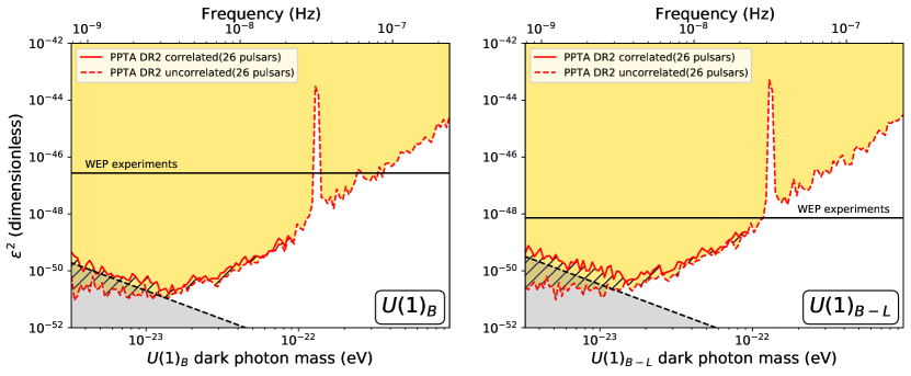
Figure 1: Constraints on the dark photon mass $m_{A}$ and the coupling constant $\epsilon^{2}$ for the $U(1)_{B}$ (left) and $U(1)_{B-L}$ (right) gauge groups. The red solid and dashed lines are derived in this work using the PPTA DR2 data, under the assumptions that the dark photon field polarizations are correlated and uncorrelated among various pulsars, respectively. The horizontal solid line is the limit from the MICROSCOPE WEP experiment MICROSCOPE . The black dashed line and the gray shaded region indicate the parameter space where the gravitational effect (studied in Refs. Porayko2018 ; gw_effect_1 ; gw_effect_2 ) dominates over the gauge interaction (studied here), for pulsar timing observations. More details about the WEP experiments and gravitational effects are presented in the Supplemental Material supp . Note that in the WEP experiments, the dark photon is not required to be the dark matter.

Statistical analysis — We perform a likelihood-ratio test, which assesses the goodness of fit using the following statistic

$$\lambda_{\rm LR}=2\ln\frac{\mathcal{L}_{\rm max}(\mathcal{H}_{1})}{\mathcal{L}_{\rm max}(\mathcal{H}_{0})},$$ (8)

where $\mathcal{H}_{0}$ is the null hypothesis that the timing residuals contain only the noise contributions, and $\mathcal{H}_{1}$ is the signal hypothesis that the DPDM signal is present. In both hypotheses the noise parameters $\boldsymbol{\vartheta}_{\rm W}$ (white noise parameters), $\boldsymbol{\vartheta}_{\rm SN}$ (spin noise parameters), $\boldsymbol{\vartheta}_{\rm DM}$ (dispersion-measure noise parameters), and $\boldsymbol{\vartheta}_{\rm BN}$ (band noise parameters) are fixed at their best-fit values obtained from single pulsar analyses. The free parameters include $\boldsymbol{\vartheta}_{\rm BE}$ (Bayes ephemeris parameters, vary in both $\mathcal{H}_{0}$ and $\mathcal{H}_{1}$; see Ref. bayes_ephmeris for details) and $\boldsymbol{\vartheta}_{\rm DPDM}$ (DPDM parameters, vary only in $\mathcal{H}_{1}$). The priors of all the parameters mentioned above are listed in Supplemental Table S2 supp .

We adopt the Bayesian approach to derive the constraints on the DPDM parameters. We set the upper limit on the coupling constant, $\bar{\epsilon}$, at 95% credibility as

$$0.95=\int_{0}^{\overline{\epsilon}}P(\epsilon)d\epsilon\int\mathcal{L}(\epsilon,\boldsymbol{\vartheta}^{\prime}_{\rm DPDM},\boldsymbol{\vartheta}_{\rm BE})P(\boldsymbol{\vartheta}^{\prime}_{\rm DPDM})P(\boldsymbol{\vartheta}_{\rm BE})\times$$

$$d\boldsymbol{\vartheta}^{\prime}_{\rm DPDM}d\boldsymbol{\vartheta}_{\rm BE},$$ (9)

where $\boldsymbol{\vartheta}^{\prime}_{\rm DPDM}$ are the DPDM parameters excluding $m_{A}$ and $\epsilon$, and $P$ are the prior probabilities of those parameters (see Supplemental Table S2 supp ). Here the dark photon mass $m_{A}$ is singled out from $\boldsymbol{\vartheta}_{\rm DPDM}$ as we search for possible signals for a given range of masses. In the computation of the upper limits, we fix both the white noise and the red noise parameters as their best-fit values obtained in single-pulsar analyses.

Results and discussion — Our main results about the $95\%$ upper limits on the coupling constant $\epsilon^{2}$, where $\epsilon$ is the dimensionless coupling constant $\epsilon$ and $\epsilon e$ is the coupling strength of the $U(1)_{B}$ or $U(1)_{B-L}$ interaction with $e$ being the electromagnetic coupling, are shown in Fig. 1. For comparison, the constraints on these parameters from experiments testing the weak equivalence principle (WEP), e.g., Ref. MICROSCOPE , are also presented. See the Supplemental Material supp for a description of the WEP results. We find that our study imposes significantly improved limits in the low-mass region with $m_{A}\lesssim 3\times 10^{-22}$ eV for $U(1)_{B}$ and $m_{A}\lesssim 10^{-22}$ eV for $U(1)_{B-L}$. Compared with the WEP results, the PPTA constraints on $\epsilon$ are stronger by one to two orders of magnitude.

We find that for a few particular frequencies, the signal hypothesis fits the PPTA DR2 data better than the null hypothesis. The strongest “signal” is at $f\simeq 1.02\times 10^{-7}~{}{\rm Hz}$. The corresponding $m_{A}$ and $\epsilon$ are given in Supplemental Table S3 supp . We note that the favored value of the coupling constant has already been ruled out by existing WEP experiments MICROSCOPE . Therefore, it may be due to some unmodeled noise effect. A similar spurious signal also appeared in the analysis Ref. Porayko2018 , which was speculated to be caused by the unmodeled perturbations of Solar System barycenter from Mercury.

In order to have a better understanding of the “signal” at $f\simeq 1.02\times 10^{-7}~{}{\rm Hz}$, we reduce the number of pulsars and perform a consistency test. We choose two sets of pulsars: The first one includes five pulsars that contribute the most to this strongest “signal”, the second one is the same except that we do not included PSR J0437-4715. Additionally, we allow red-noise parameters $\boldsymbol{\vartheta}_{\rm SN}$, $\boldsymbol{\vartheta}_{\rm DM}$, and $\boldsymbol{\vartheta}_{\rm BN}$ to vary along with $\boldsymbol{\vartheta}_{\rm DPDM}$ and $\boldsymbol{\vartheta}_{\rm BE}$. We calculate the Bayes factor between the null and the signal hypothesis. We find that the “signal” is mainly contributed by PSR J0437-4715. For the analysis with the other four pulsars excluding PSR J0437-4715 gives a logarithmic Bayes factor of 37 in favor of the $\mathcal{H}_{1}$ hypothesis at $f\simeq 6.58\times 10^{-8}~{}{\rm Hz}$, which is significantly smaller than the five-pulsar analysis. The results of the tests are presented in Supplemental Table S4 supp . Note also that the best-fit frequency differs from that of the five-pulsar analysis, and the best-fit coupling constant lies above the WEP upper limit, indicating that this may be due to unmodelled noise. More careful studies need to be carried out in the future to understand the sources of these systematics.

We note that the mass range with the strongest constraint is below the typical fuzzy dark matter mass ($10^{-22}$ eV). Currently there is no consensus on the constraints on the mass of the fuzzy dark matter. The stellar kinematics of dwarf spheroidal galaxies tend to favor a lower mass Gonzalez2017 ; Kendal2020 (a few times of $10^{-23}$ eV), while the halo mass function derived from the Lyman-$\alpha$ forest suggests a higher lower limit Hui2017 ; Armengaud2017 ($\gtrsim 10^{21}$ eV). Most of these constraints rely on assumptions about the structure formation in the fuzzy dark matter scenario. More detailed studies of the interplay between the fuzzy dark matter and the baryonic matter, such as the dark matter-to-baryon mass ratio or various baryonic effects in fuzzy dark matter simulations, are required to reach a robust and consistent result.

The gray shaded regions in Fig. 1 indicate the parameter space for which the “gravitational effect” due to the space-time metric oscillation induced by the wavelike DPDM field dominates over the gauge interaction discussed in this work. See the Supplemental Material supp for more details of the estimate of the gray regions. In such parameter regions, dedicated analysis with both effects being included in the signal model is required and will be studied in future work.

Summary — Ultralight fuzzy dark matter is proposed as an attractive candidate of dark matter in the universe which helps solve the small-scale crises of the classical cold dark matter scenario. Using the precise timing observations of 26 pulsars by the PPTA project, we study the possible couplings between ultralight dark matter and ordinary matter. Taking the DPDM as an example, we obtain by far the strongest constraints on the parameters of the DPDM. The upper limits on the dimensionless coupling constant $\epsilon$ derived in our study are improved by up to two orders of magnitude when the dark photon mass is smaller than $3\times 10^{-22}$ eV ($10^{-22}$ eV) for the $U(1)_{B}$ ($U(1)_{B-L}$) scenario.

The search sensitivity for the DPDM is expected to improve significantly in the near future as more pulsars are monitored with continually extending data spans by the worldwide PTA campaigns including the PPTA, the North American Nanohertz Observatory for Gravitational Waves (NANOGrav NANOGrav ), and the European PTA (EPTA EPTA ), which have jointly formed the International PTA (IPTA IPTA ). The Five-hundred-meter Aperture Spherical Telescope (FAST FAST ) and the Square Kilometer Array (SKA SKA ) are also expected to join the IPTA collaboration. These efforts are likely to bring revolutionary progress in studying a wide range of dark matter models, and more generally in answering the related fundamental questions in physics.

Acknowledgements This work is supported by the National Natural Science Foundation of China (No. 11722328, No. 11851305, No. 12003069, No. 11947302, No. 11690022, No. 11851302, No. 11675243, and No. 11761141011). X.X. is supported by Deutsche Forschungsgemeinschaft under Germany’s Excellence Strategy EXC2121 “Quantum Universe” 390833306. Q.Y. is supported by the Key Research Program of the Chinese Academy of Sciences (No. XDPB15) and the Program for Innovative Talents and Entrepreneur in Jiangsu. J.S. is supported by the Strategic Priority Research Program of the Chinese Academy of Sciences under Grants No. XDB21010200 and No. XDB23000000. X.J.Z., A.D.C., B.G., D.J.R. and R.M.S. are supported by ARC CE170100004. Z.Q.X. is supported by the Entrepreneurship and Innovation Program of Jiangsu Province. Y.Z. is supported by U.S. Department of Energy under Award Number DESC0009959. R.M.S. is the recipient of ARC Future Fellowship FT190100155. J.W. is supported by the Youth Innovation Promotion Association of Chinese Academy of Sciences. S.D. is the recipient of an Australian Research Council Discovery Early Career Award (DE210101738) funded by the Australian Government. The Parkes radio telescope is part of the Australia Telescope, which is funded by the Commonwealth Government for operation as a National Facility managed by CSIRO.

Supplemental Material

.1 Noise model

Following Porayko2018 , we assume ${\Delta t}_{\rm Noise}$ follows a multivariate Gaussian distribution with a covariance matrix $\boldsymbol{C}^{\rm tot}$. In the most general case, for each pulsar, $\boldsymbol{C^{\rm tot}}$ contains four terms:

$$\boldsymbol{C^{\rm tot}}=\boldsymbol{N}+\boldsymbol{C}^{\rm SN}+\boldsymbol{C}^{\rm DM}+\boldsymbol{C}^{\rm BN},$$ (10)

where $\boldsymbol{N}$ accounts for white noise, $\boldsymbol{C}^{\rm SN}$, $\boldsymbol{C}^{\rm DM}$ and $\boldsymbol{C}^{\rm BN}$ arise from red-noise processes. $\boldsymbol{C}^{\rm SN}$ is the spin noise that describes the time-correlated spin noise which might be induced by rotational irregularities of the pulsar. $\boldsymbol{C}^{\rm DM}$ accounts for the time variations of the dispersion measures. $\boldsymbol{C}^{\rm BN}$ is the band noise which is used to account for unknown additional red noise that is only present in a specific radio-frequency band red_noise_exp_2 . In our analysis, we only include band noise for two pulsars that are known to exhibit significant band noise red_noise_exp_2 , PSR J0437-4715 and J1939+2124. We apply the band noise for these two pulsars in four bands: 10 cm, 20 cm, 40 cm and 50 cm. All the terms in Eq. (10) are $n\times n$ matrices, with $n$ being the number of ToAs for each pulsar. In practice, the white noise of the actual timing data is usually larger than the ToA measurement uncertainties. Empirically, for each receiver/backend system and each pulsar, a re-scaling factor EFAC (Error FACtor) is multiplied to the measurement uncertainty, and an extra white noise component EQUAD (Error added in QUADrature) is also included S (1, 2, 3). The rescaled ToA uncertainty $\sigma_{s}$ is related to the original uncertainty $\sigma$

$$\sigma_{s}^{2}=({\tt EFAC}\times\sigma)^{2}+{\tt EQUAD}^{2}.$$ (11)

We model the power spectra of the spin noise, band noise and dispersion-measure noise as power-law functions,

$$P(f)=\frac{A^{2}}{12\pi}\left(\frac{f}{\rm yr^{-1}}\right)^{-\gamma}~{}{\rm yr}^{3},$$ (12)

where $A$ and $\gamma$ are the noise amplitude and noise spectral index at a reference frequency of ${\rm yr^{-1}}$, respectively. The noise covariance matrices are,

$$\boldsymbol{C}_{ij}^{\rm SN,BN}=\int_{f_{L}}{\rm d}fP(f)\cos\left(2\pi f(t_{i}-t_{j})\right),$$ (13)

$$\boldsymbol{C}_{ij}^{\rm DM}=\int_{f_{L}}{\rm d}fP(f)\left(\frac{\nu^{\rm ref}}{\nu^{\rm obs}_{i}}\right)^{2}\left(\frac{\nu^{\rm ref}}{\nu^{\rm obs}_{j}}\right)^{2}\cos\left(2\pi f(t_{i}-t_{j})\right),$$ (14)

here $t_{i}$ and $t_{j}$ are $i$-th and $j$-th ToAs, $\nu^{\rm obs}_{i}$ and $\nu^{\rm obs}_{j}$ are their respective radio frequencies, $f_{L}$ is the low-frequency cutoff, $\nu^{\rm ref}=1400$ MHz is the reference radio frequency. Earlier work shows that setting $f_{L}=1/T$, with $T$ being the observational time interval, is sufficient for pulsar timing analysis due to the fitting for the quadratic spin-down in the timing model red_noise_1 ; temponest . Note that in Eq. (13), the elements of band-noise covariance matrics is non-zero only when radio frequencies of $i$-th and $j$-th ToAs belong to the same frequency band.

We adopt the “time-frequency” method to calculate the integral in Eq. (13,14). Namely, we approximate the integral as a discrete summation of different Fourier frequency modes. In this approximation, a uniform interval of Fourier frequency modes is usually adopted up to an upper limit. One may choose an interval of ${\rm d}f\equiv\Delta f=1/T$, which we call “T uniform”. However, such a choice is sub-optimal red_noise_2 . Instead, we adopt the “2T uniform” sampling where $\Delta f=1/(2T)$ for the approximation of Eq. (13,14). We found a better approximation is achieved with the “2T uniform” interval. On this basis, we find that additional periodic patterns may appear due to the approximation, when $\gamma$ is small. We also compare the influence of the total number of Fourier frequency modes (time-frequency modes) $M$ when $M=30$ and $M=40$, and find that the frequencies of their periodic patterns are different. This is used to remove the potential fake signal introduced during this calculation. The discussions above are demonstrated in Fig. S1.

In the “time-frequency” method, the covariance matrices in Eq. (13, 14) can be rewritten as

$$\boldsymbol{C} \approx \boldsymbol{C}^{(S)}+\boldsymbol{C}^{(C)}=\boldsymbol{F}^{(S)}\boldsymbol{\Phi}(\boldsymbol{F}^{(S)})^{T}+\boldsymbol{F}^{(C)}\boldsymbol{\Phi}(\boldsymbol{F}^{(C)})^{T},$$ (15)

with $\boldsymbol{\Phi}_{\alpha\beta}=(A^{2}/12\pi^{2})(1/T)(f_{\alpha})^{-\gamma}\delta_{\alpha\beta}$. For spin and band noise, $\boldsymbol{F}^{(S)}_{i\alpha}=\sin\left(2\pi f_{\alpha}t_{i}\right)$ and $\boldsymbol{F}^{(C)}_{i\alpha}=\cos\left(2\pi f_{\alpha}t_{i}\right)$; For dispersion-measure noise $\boldsymbol{F}^{(S)}_{i\alpha}=(\nu^{\rm ref}/\nu^{\rm obs}_{i})^{2}\sin\left(2\pi f_{\alpha}t_{i}\right)$ and $\boldsymbol{F}^{(C)}_{i\alpha}=(\nu^{\rm ref}/\nu^{\rm obs}_{i})^{2}\cos\left(2\pi f_{\alpha}t_{i}\right)$. Here $i$ is the index for ToAs, and $\alpha$ is used to label the discretized Fourier frequency. We follow Ref. Porayko2018 in terms of the definition and calculation of the likelihood function.

The parameter description and prior ranges of the noise model is given in Table S2. In Table S1 we also present the posterior credible intervals for spin noise and dispersion-measure noise based on the results of single pulsar analyses, where we analyze the noise properties of each pulsar independently. In Bayesian analyses detailed below, we fix the noise parameters at their maximal likelihood values obtained from single pulsar analyses in some cases to reduce the computational costs. They are referred to as the ”best fit” parameter values, which are available in our code repository.

Figure S1: The comparison between the 2T uniform approximation and T uniform approximation of Eq. (13) with different $\gamma$. The y-axis is the value of the noise covariance matrix element at different $\tau_{ij}$. The red thick lines are the true values of Eq. (13) without disretization and high frequency cut. In first two panels, the solid black lines are the results from the 2T uniform approximation, the dashed black lines are from the T uniform approximation. In the last panel, we show the 2T uniform approximation of Eq. (13) when the time-frequency modes $M$ equals to $30$ and $40$ with solid gray line and dashed black line respectively. As an illustration, we choose $T\approx 13.1$ years, which is shown as the vertical dashed gray line in these plots. The approximation may create additional periodic patterns. To remove the fake signal, we change the number of time-frequency modes from $M=30$ to $M=40$ in the likelihood-ratio test. If the excess only exists in one of the choices of $M$, it will not be identified as our signal.

.2 Simulation of the DPDM background

Here we provide details on how to simulate the DPDM background. The interference among the wave-functions of these dark photon particles induces fluctuations on the dark matter field strength. Here we study this amplitude distribution, and it will be used to inform our priors in the statistical analysis. In addition, by studying the spatial correlations among various quantities of the dark photon background, we demonstrate the concept of coherence length. Within the coherence length, the DPDM can be approximated as a plane wave, whereas this approximation breaks down once the spatial separation becomes larger.

The dark photon background $\boldsymbol{A}^{(tot)}$ can be modeled as the summation of many, $N\gg 1$, freely propagating planewaves,

$$\boldsymbol{A}^{(tot)}(t,\boldsymbol{x})=\sum_{n=1}^{N}\boldsymbol{A}^{(n)}(t,\boldsymbol{x})=\sum_{n=1}^{N}\boldsymbol{A}_{0}^{(n)}\sin(\omega^{(n)}t-\boldsymbol{k}^{(n)}\cdot\boldsymbol{x}+\alpha^{(n)}),$$ (16)

where $n$ is the index for each dark photon particle and $\alpha^{(n)}$ is the phase term in a plane wave. $\boldsymbol{A}_{0}^{(n)}$ is the gauge potential vector, whose magnitude is the same for all particles, but the direction is isotropically distributed. $\omega^{(n)}$ and $\boldsymbol{k}^{(n)}$ are the particle’s energy and momentum, distributed according to Boltzmann velocity distribution with virial velocity $v_{vir}\sim 220$ km/s.

The normalization of the dark photon field is determined by the local dark matter energy density $\rho_{0}$,

$$\int_{0}^{T}{\rm d}t\int_{V}{\rm d}^{3}\boldsymbol{x}~{}\frac{1}{2}m_{A}^{2}|\boldsymbol{A}^{(tot)}(t,\boldsymbol{x})|^{2}=(VT)~{}\rho_{0},$$ (17)

where $V$ and $T$ need to be sufficiently large, much larger than the coherence volume and time. Since $v_{vir}\ll c$, we have $\omega^{(n)}\simeq m_{A}$. For the mass range that we are interested in, the coherence time is much larger than the observation time. Also as discussed previously, the phase variations, induced by the motions of pulsars and the Earth in the Galaxy during the period of observation, are negligible. Thus in our analysis, we can approximate the wave-function for the DPDM as

$$A_{i}^{(tot)}(\boldsymbol{x})=A_{0,i}^{(tot)}(\boldsymbol{x})\sin(m_{A}t+\alpha_{i}(\boldsymbol{x})),$$ (18)

where the index $i$ labels the spatial component of the dark photon field, i.e. $\{x,y,z\}$. The averaged magnitude of the gauge potential component can written as

$$E[(A^{(tot)}_{0,i})^{2}]=\frac{2}{3}\frac{\rho_{0}}{m_{A}^{2}}.$$ (19)

For simplicity we introduce a normalized DPDM amplitude

$$\tilde{A}^{(\rm{tot})}_{0,i}\equiv\frac{\sqrt{3}m_{A}}{\sqrt{2\rho_{0}}}A^{(\rm{tot})}_{0,i}.$$ (20)

To study the statistic behaviors of the DPDM, we set $N=2^{15}$ and simulate the background field for $10^{5}$ times. This ensures the results we obtain are statistically stable. We first focus on the DPDM amplitude. In the left panel of Fig. S2, we show the distribution of $(\tilde{A}^{(\rm{tot})}_{0,x})^{2}$ at $\boldsymbol{x}=\boldsymbol{0}$. This distribution can be well fit by an exponential function, which will be used as the prior probability of $(\tilde{A}^{(\rm{tot})}_{0,i})^{2}$ in our Bayesian analysis.

Next we study the coherence of the dark photon field as a function of the spatial separation between two points. The coherence between two quantities, $X$ and $Y$, can be described by their two-point correlation function as

$$corr(X,Y)=\frac{E[(X-\mu_{X})(Y-\mu_{Y})]}{\sigma_{X}\sigma_{Y}},$$ (21)

where $\mu_{X}$, $\mu_{Y}$ are expectation values, and $\sigma_{X}$, $\sigma_{Y}$ are standard deviations. Let us consider $X\in\{\tilde{A}^{(\rm{tot})}_{0,i}(0,0,0),~{}\alpha_{i}(0,0,0)\}$ and $Y\in\{\tilde{A}^{(\rm{tot})}_{0,i}(d,0,0),~{}\alpha_{i}(d,0,0)\}$, where $d$ represents the separation between two points. In the right panel of Fig. S2, we show $corr(X,Y)$ as a function of spatial separation. Here we clearly see that the correlation function reduces significantly once the spatial separation is longer than the coherence length, i.e., the de Broglie wavelength. We compare our result with the separations among the Earth and pulsars. We find that when $m_{A}>10^{-22}$ eV, it is safe to assume that the dark photon field at these locations are completely uncorrelated.

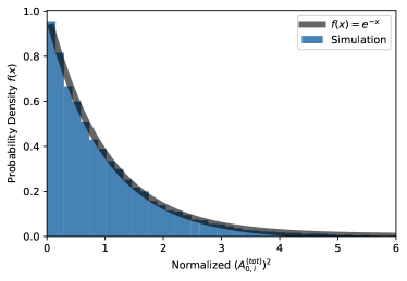
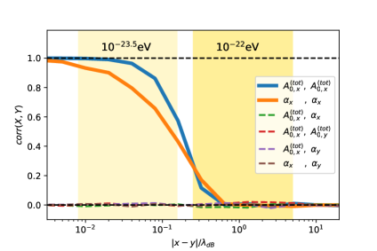
Figure S2: Left: the probability distribution of normalized $A^{(tot)}_{0,i}$ ($\tilde{A}^{(tot)}_{0,i}$) from the simulation. The black curve shows an exponential function fit. Right: the correlations between different variables as functions of spatial separation. $\lambda_{dB}=2\pi/(m_{A}v_{vir})$ is the de Broglie wavelength. The correlation is non-zero only when the random variables $X$ and $Y$ have the same spatial indices, and thus the three spatial components of the DPDM field are always independent. The two yellow bands indicate the distances between the Earth and most pulsars ($0.1-2$ kpc) when $m_{A}=10^{-23.5}$ eV and $m_{A}=10^{-22}$ eV.

.3 Limits from the WEP experiment

The experiments testing the weak equivalence principle (WEP) can also impose stringent constraints on the coupling constant of the $U(1)_{B}$ or $U(1)_{B-L}$ gauge force. In the WEP experiments, the dark photon is not required to be the dark matter. Here we compare our results with those obtained by WEP experiments. For the mass regime that we are interested in this study, the best limit is given by the satellite experiment, MICROSCOPE MICROSCOPE . The effect is characterized by the Eötvös parameter as

$$\eta_{\rm E-s}\simeq\frac{e^{2}\epsilon^{2}}{4\pi G}\left[\left(\frac{q_{1}}{m_{1}}\right)-\left(\frac{q_{2}}{m_{2}}\right)\right]\frac{q_{E}}{m_{E}},$$ (22)

where $q_{1,2,E}$ and $m_{1,2,E}$ are the “dark charges” and masses of the two test bodies in the MICROSCOPE satellite and the Earth, respectively. The best sensitivity achieved by the MICROSCOPE experiment MICROSCOPE is $|\eta|<2.7\times 10^{-14}$ at $2\sigma$ level. This can be translated to constraints on coupling constants as $\epsilon>10^{-23.28}$ for $U(1)_{B}$ and $\epsilon>10^{-24.07}$ for $U(1)_{B-L}$. The results are consistent with Ref. Pierre1 . In Fig. 1, we find our results improves upon that of MICROSCOPE when $m_{A}\lesssim 3\times 10^{-22}$ eV for $U(1)_{B}$ and $m_{A}\lesssim 10^{-22}$ eV for $U(1)_{B-L}$, by up to two orders of magnitudes.

.4 Gravitational effect of DPDM on the ToA

The quantum pressure of the ultralight bosonic dark matter field can induce a periodic oscillation of the metric. This will affect the propagation of photons and lead to detectable oscillatory effects at pulsar timing experiments. Such an effect has been studied in Refs. gw_effect_1 ; Porayko2018 in the case of ultralight scalar field. Ultralight vector field, such as the dark photon, can also be searched in this way. Thus it is instructive to compare this pure gravitational effect with the effect studied in this paper.

According to Refs. gw_effect_1 ; gw_effect_2 , the timing residual caused by the oscillating quantum pressure can be written as,

$$\Delta t_{\rm scalar}=\frac{\Psi_{c}}{\pi f}\times\sin(\Delta\alpha_{p})\cos(2\pi ft+2\alpha_{e}+\Delta\alpha_{p}),$$ (23)

$$\Delta t_{\rm vector}\leq 3\times\Delta t_{\rm scalar}.$$ (24)

Here $\Psi_{c}\equiv G\rho_{0}/(\pi f^{2})$ with $f=m_{\rm DM}/\pi$, and $m_{\rm DM}$ is the mass of the dark matter particle. The root-mean-square value of $\Delta t$ is

$$\sqrt{\langle\Delta t_{\rm scalar}^{2}\rangle}\simeq 0.5~{}\pi\times\frac{G\rho_{0}}{m_{\rm DM}^{3}},$$ (25)

$$\sqrt{\langle\Delta t_{\rm vector}^{2}\rangle}\simeq 1.5~{}\pi\times\frac{G\rho_{0}}{m_{\rm DM}^{3}},$$ (26)

where we take the maximal value of vector dark matter’s timing residual. Meanwhile, the effect induced by the gauge coupling of the DPDM has the root-mean-square value as

$$\sqrt{\langle(\Delta t_{\rm dp}^{(B)})^{2}\rangle}\simeq 0.577\ \epsilon e\frac{\sqrt{2\rho_{0}}}{m_{A}^{2}},$$ (27)

$$\sqrt{\langle(\Delta t_{\rm dp}^{(B-L)})^{2}\rangle}\simeq 0.456\ \epsilon e\frac{\sqrt{2\rho_{0}}}{m_{A}^{2}}.$$ (28)

where the prefactors are obtained through our numerical simulation. By comparing the root-mean-square value of these two effects, we find that the gauge interaction of the dark photon induces a stronger effect when $\epsilon\times m_{A}/{\rm eV}>10^{-48.35}$ for $U(1)_{B}$ and $10^{-48.24}$ for $U(1)_{B-L}$. This comparison is shown as the black dashed line in Fig. 1.

Table S1: Properties of the 26 pulsars used in this analysis. This table doesn’t include the band noise properties of pulsars J0437-4715 and J1939+2134.

Pulsars	$N_{\rm obs}$	$T$ (years)	$\bar{\sigma}\times 10^{-6}$ (s)	$\log A_{\rm SN}$	$\gamma_{\rm SN}$	$\log A_{\rm DM}$	$\gamma_{\rm DM}$
J0437-4715	29262	15.03	0.296	$-15.76^{+0.17}_{-0.18}$	$6.63^{+0.17}_{-0.13}$	$-13.05^{+0.10}_{-0.08}$	$2.26^{+0.32}_{-0.44}$
J0613-0200	5920	14.20	2.504	$-14.63^{+0.77}_{-0.68}$	$4.93^{+1.33}_{-1.61}$	$-13.02^{+0.08}_{-0.08}$	$0.95^{+0.33}_{-0.31}$
J0711-6830	5547	14.21	6.197	$-12.85^{+0.14}_{-0.16}$	$0.97^{+0.64}_{-0.55}$	$-14.54^{+0.72}_{-0.89}$	$4.43^{+1.68}_{-1.72}$
J1017-7156	4053	7.77	1.577	$-12.89^{+0.07}_{-0.07}$	$0.54^{+0.53}_{-0.37}$	$-12.72^{+0.06}_{-0.06}$	$2.18^{+0.45}_{-0.44}$
J1022+1001	7656	14.20	5.514	$-12.79^{+0.12}_{-0.13}$	$0.54^{+0.55}_{-0.37}$	$-13.04^{+0.10}_{-0.12}$	$0.58^{+0.47}_{-0.36}$
J1024-0719	2643	14.09	4.361	$-14.28^{+0.27}_{-0.20}$	$6.51^{+0.35}_{-0.60}$	$-14.53^{+0.54}_{-0.56}$	$5.22^{+1.14}_{-1.18}$
J1045-4509	5611	14.15	9.186	$-12.75^{+0.24}_{-0.40}$	$1.58^{+1.28}_{-0.93}$	$-12.18^{+0.09}_{-0.08}$	$1.86^{+0.36}_{-0.32}$
J1125-6014	1407	12.34	1.981	$-12.64^{+0.11}_{-0.12}$	$0.51^{+0.55}_{-0.37}$	$-13.14^{+0.19}_{-0.21}$	$3.36^{+0.73}_{-0.66}$
J1446-4701	508	7.36	2.200	$-16.46^{+2.88}_{-3.17}$	$2.74^{+2.49}_{-1.89}$	$-13.49^{+0.32}_{-1.87}$	$2.48^{+1.92}_{-1.45}$
J1545-4550	1634	6.97	2.249	$-17.33^{+2.50}_{-2.55}$	$3.25^{+2.45}_{-2.18}$	$-13.40^{+0.24}_{-0.38}$	$3.90^{+1.61}_{-1.09}$
J1600-3053	7047	14.21	2.216	$-17.63^{+2.10}_{-2.29}$	$3.28^{+2.34}_{-2.15}$	$-13.27^{+0.12}_{-0.13}$	$2.79^{+0.43}_{-0.40}$
J1603-7202	5347	14.21	4.947	$-12.82^{+0.14}_{-0.16}$	$1.01^{+0.67}_{-0.60}$	$-12.66^{+0.10}_{-0.09}$	$1.44^{+0.40}_{-0.38}$
J1643-1224	5941	14.21	4.039	$-12.32^{+0.08}_{-0.09}$	$0.51^{+0.42}_{-0.34}$	$-12.27^{+0.07}_{-0.07}$	$0.55^{+0.32}_{-0.29}$
J1713+0747	7804	14.21	1.601	$-14.09^{+0.25}_{-0.38}$	$2.98^{+1.00}_{-0.64}$	$-13.35^{+0.08}_{-0.08}$	$0.53^{+0.32}_{-0.31}$
J1730-2304	4549	14.21	5.657	$-17.39^{+2.39}_{-2.51}$	$3.05^{+2.59}_{-2.12}$	$-14.11^{+0.40}_{-0.57}$	$4.22^{+1.42}_{-1.04}$
J1732-5049	807	7.23	7.031	$-16.51^{+3.04}_{-2.97}$	$3.29^{+2.37}_{-2.97}$	$-13.38^{+0.54}_{-0.84}$	$4.07^{+1.96}_{-1.93}$
J1744-1134	6717	14.21	2.251	$-13.39^{+0.14}_{-0.15}$	$1.49^{+0.66}_{-0.57}$	$-13.35^{+0.09}_{-0.09}$	$0.86^{+0.40}_{-0.33}$
J1824-2452A	2626	13.80	2.190	$-12.56^{+0.13}_{-0.12}$	$3.61^{+0.41}_{-0.39}$	$-12.18^{+0.11}_{-0.10}$	$1.64^{+0.46}_{-0.59}$
J1832-0836	326	5.40	1.430	$-16.47^{+2.63}_{-3.09}$	$3.66^{+2.33}_{-2.52}$	$-13.07^{+0.24}_{-0.63}$	$3.77^{+2.00}_{-1.05}$
J1857+0943	3840	14.21	5.564	$-14.76^{+0.74}_{-0.50}$	$5.75^{+0.91}_{-1.53}$	$-13.40^{+0.20}_{-0.25}$	$2.66^{+0.83}_{-0.67}$
J1909-3744	14627	14.21	0.672	$-13.60^{+0.13}_{-0.12}$	$1.60^{+0.43}_{-0.46}$	$-13.48^{+0.09}_{-0.08}$	$0.69^{+0.38}_{-0.35}$
J1939+2134	4941	14.09	0.468	$-14.38^{+0.22}_{-0.18}$	$6.24^{+0.49}_{-0.62}$	$-11.59^{+0.07}_{-0.07}$	$0.13^{+0.19}_{-0.10}$
J2124-3358	4941	14.21	8.863	$-14.79^{+0.82}_{-0.67}$	$5.07^{+1.37}_{-1.97}$	$-13.35^{+0.18}_{-0.33}$	$0.95^{+1.11}_{-0.66}$
J2129-5721	2879	13.88	3.496	$-15.48^{+1.92}_{-3.54}$	$2.91^{+2.29}_{-1.83}$	$-13.31^{+0.13}_{-0.14}$	$1.07^{+0.65}_{-0.65}$
J2145-0750	6867	14.09	5.086	$-12.82^{+0.10}_{-0.11}$	$0.62^{+0.50}_{-0.40}$	$-13.33^{+0.14}_{-0.16}$	$1.38^{+0.54}_{-0.55}$
J2241-5236	5224	8.20	0.830	$-13.40^{+0.09}_{-0.08}$	$0.44^{+0.40}_{-0.30}$	$-13.79^{+0.10}_{-0.10}$	$1.42^{+0.61}_{-0.59}$

Table S2: The model parameters of the analysis. $\tilde{A}_{0}^{p}$ and $\tilde{A}_{0}^{e,i}$ are normalized amplitudes of the DPDM field. We consider only one set of DPDM parameters for each pulsar, $\tilde{A}_{0}^{p}$ and $\alpha_{p}$, while all three spatial components for the Earth are included. This is because only the DPDM oscillation along the line of sight is detectable. * suggests that the parameters only exist in the uncorrelated case.

	Parameter	Prior	Description
White Noise $\boldsymbol{\vartheta}_{\rm W}$	EFAC	U[$0.01$,$10$]	one per backend
	EQUAD	log-U [$10^{-10}$,$10^{-4}$]	one per backend
Spin Noise $\boldsymbol{\vartheta}_{SN}$	$\gamma_{\rm SN}$	U[$0$,$7$]	one per pulsar
	$A_{\rm SN}$	log-U[$10^{-21}$,$10^{-9}$]	one per pulsar
DM Noise $\boldsymbol{\vartheta}_{\rm DM}$	$\gamma_{\rm DM}$	U[$0$,$7$]	one per pulsar
	$A_{\rm DM}$	log-U[$10^{-21}$,$10^{-9}$]	one per pulsar
Band Noise $\boldsymbol{\vartheta}_{\rm BN}$ for J0437 and J1939	$\gamma_{\rm BN}$	U[$0$,$7$]	one per band
	$A_{\rm BN}$	log-U[$10^{-21}$,$10^{-9}$]	one per band
Dark photon Parameters $\boldsymbol{\vartheta}_{\rm DPDM}$	$\alpha_{p}$	U[$0$,$2\pi$]	one per pulsar
	$\alpha_{e}^{i}$	U[$0$,$2\pi$]	three per PTA
	$(\tilde{A}_{0}^{p})^{2}$	$f(x)=e^{-x}$	one per pulsar*
	$(\tilde{A}_{0}^{e,i})^{2}$	$f(x)=e^{-x}$	three per PTA
	$\epsilon$	log-U[$10^{-28}$,$10^{-16}$]	one per PTA
	$m_{A}$	log-U[$10^{-23.5}$,$10^{-21}$]	one per PTA
BayesEphem Parameters $\boldsymbol{\vartheta}_{\rm BE}$	$z_{\rm drift}$	U[$-10^{-9}$,$10^{-9}$]	one per PTA
	$\Delta M_{\rm Jupiter}$	N$(0,1.5\times 10^{-11})$	one per PTA
	$\Delta M_{\rm Saturn}$	N$(0,8.2\times 10^{-12})$	one per PTA
	$\Delta M_{\rm Uranus}$	N$(0,5.7\times 10^{-11})$	one per PTA
	$\Delta M_{\rm Neptune}$	N$(0,7.9\times 10^{-11})$	one per PTA
	${\rm PCA}_{i}$	U[$-0.05$,$0.05$]	six per PTA

Table S3: The best-fit dark photon parameters that favor the $\mathcal{H}_{1}$ hypothesis with a total of 26 pulsars.

Interaction	$m_{A}{\rm(eV)}$	$f{\rm(Hz)}$	$\epsilon$	$\lambda_{LR}^{max}$
$U(1)_{B}$	$10^{-21.37}$	$1.02\times 10^{-7}$	$10^{-22.68}$	472
$U(1)_{B-L}$	$10^{-21.37}$	$1.02\times 10^{-7}$	$10^{-22.87}$	498

Table S4: The Bayes factor and maximal-likelihood parameters with different choices of pulsars and DPDM parameters. As a demonstration, here we only show the results for the $U(1)_{B}$ model with uncorrelated dark photon background field. The “5 pulsars” includes J0437-4715, J1022+1001, J1744-1134, J1909-3744 and J2145-0750, while the “4 pulsars” excludes J0437-4715 in the analysis.

Target	Range of $m_{A}{\rm(eV)}$	ln(Bayes Factor)	Best Fit Parameters	$\lambda_{LR}^{max}$
			$(m_{A}$,$\epsilon,f)$
5 pulsars	$[10^{-23.5},10^{-22}]$	3.5	$(10^{-22.98}{\rm eV},10^{-24.60},2.51\times 10^{-9}{\rm Hz})$	7.2
	$[10^{-22},10^{-21}]$	207.0	$(10^{-21.37}{\rm eV},10^{-22.66},1.02\times 10^{-7}{\rm Hz})$	458
	$[10^{-23.5},10^{-21}]$	212.3
4 pulsars	$[10^{-23.5},10^{-21}]$	37.2	$(10^{-21.56}{\rm eV},10^{-22.89},6.58\times 10^{-8}{\rm Hz})$	114

References

- (1) N. A. Bahcall, J. P. Ostriker, S. Perlmutter, and P. J. Steinhardt, The Cosmic triangle: Revealing the state of the universe, Science, 284, 1481-1488 (1999).
- (2) D. H. Weinberg, J. S. Bullock, F. Governato, R. K. de Naray, and A. H. G. Peter, Cold dark matter: Controversies on small scales, Proc. Nat. Acad. Sci. U. S. A., 112, 12249-12255 (2015).
- (3) T. K. Chan, D. Kereš, J. Onorbe, P. F. Hopkins, A. L. Muratov, C.-A. Faucher-Giguere, and E. Quataert, The impact of baryonic physics on the structure of dark matter haloes: The view from the FIRE cosmological simulations, Mon. Not. R. Astron. Soc. 454, 2981-3001 (2015).
- (4) P. Bode, J. P. Ostriker, and N. Turok, Halo formation in warm dark matter models, Astrophys. J., 556, 93 (2001).
- (5) S. Tulin, and H. B. Yu, Dark matter self-interactions and small scale structure, Phys. Rept. , 730, 1-57 (2018).
- (6) W. Hu, R. Barkana, and A. Gruzinov, Fuzzy Cold Dark Matter: TheWave Properties of Ultralight Particles, Phys. Rev. Lett., 85, 1158-1161 (2000).
- (7) C. P. Burgess, J. P. Conlon, L.-Y. Hung, C. H. Kom, A. Maharana, and F. Quevedo, Continuous global symmetries and hyperweak interactions in string compactifications, J. High Energy Phys., 07, 073 (2008).
- (8) M. Goodsell, J. Jaeckel, J. Redondo, and A. Ringwald, Naturally light hidden photons in LARGE volume string compactifications, J. High Energy Phys., 11, 027 (2009).
- (9) M. Cicoli, M. Goodsell, J. Jaeckel, and A. Ringwald, Testing string vacua in the lab: From a hidden CMB to dark forces in flux compactifications, J. High Energy Phys., 07, 114 (2011).
- (10) In order to give a mass to the dark photon, a Higgs boson in the dark section may be introduced. Since such a Higgs is also very weakly coupled to the Standard Model sector, its existence is challenging to be tested. Furthermore, if one pushes the dark Higgs coupling to be very small, takes its vacuum expectation value to be very large, meanwhile maintains the product of these two parameters to be finite, we reach the Stueckelberg limit where the dark Higgs is very heavy and effectively decoupled from the rest of the theory, except the dark photon mass it generates.
- (11) The occupation number is , where is the local dark matter energy density.
- (12) H.-Y. Schive, T. Chiueh, and T. Broadhurst, Cosmic structure as the quantum interference of a coherent dark wave, Nature Phys., 10, 496-499 (2014).
- (13) H.-Y. Schive, M.-H. Liao, T.-P. Woo, S.-K. Wong, T. Chiueh, T. Broadhurst, and W. Y. P. Hwang, Understanding the Core-Halo Relation of Quantum Wave Dark Matter from 3D Simulations, Phys. Rev. Lett., 113, 261302 (2014).
- (14) J. Zhang, Y.-L. S. Tsai, J.-L. Kuo, K. Cheung, and M.-C. Chu, Ultralight axion dark matter and its impact on dark halo structure in N-body simulations, Astrophys. J., 853, 51 (2018).
- (15) J. F. Navarro, C. S. Frenk, and S. D. M. White, A universal density profile from hierarchical clustering, Astrophys. J., 490, 493 (1997).
- (16) L. Hui, J. P. Ostriker, S. Tremaine, and E. Witten, Ultralight scalars as cosmological dark matter, Phys. Rev. D 95, 043541 (2017).
- (17) X. Cui, A. Abdukerim, W. Chen, X. Chen, Y. Chen, B. Dong, D. Fang, C. Fu, K. Giboni, F. Giuliani, et al. (PandaX-II Collaboration), Dark Matter Results from 54-Ton-Day Exposure of PandaX-II Experiment, Phys. Rev. Lett., 119, 181302 (2017).
- (18) D. S. Akerib, S. Alsum, H. M. Araújo, X. Bai, A. J. Bailey, J. Balajthy, P. Beltrame, E. P. Bernard, A. Bernstein, T. P. Biesiadzinski, et al. (LUX Collaboration), Results from a Search for Dark Matter in the Complete LUX Exposure, Phys. Rev. Lett., 118, 021303 (2017).
- (19) E. Aprile, J. Aalbers, F. Agostini, M. Alfonsi, L. Althueser, F. D. Amaro, M. Anthony, F. Arneodo, L. Baudis, B. Bauermeister, et al. (XENON Collaboration), Dark Matter Search Results from a One Ton-Year Exposure of XENON1T, Phys. Rev. Lett., 121, 111302 (2018).
- (20) J. Bergé, P. Brax, G. Métris, M. Pernot-Borràs, P. Touboul, J.-P. Uzan, MICROSCOPE mission: First Constraints on the Violation of the Weak Equivalence Principle by a Light Scalar Dilaton, Phys. Rev. Lett., 119 231101 (2017).
- (21) T. K. Poddar, S. Mohanty, S. Jana, Vector gauge boson radiation from compact binary systems in a gauged L - L scenario, Phys. Rev. D, 100, 123023 (2019).
- (22) P. Fayet, The fifth force charge as a linear combination of baryonic, leptonic (or BL) and electric charges, Phys. Lett. B, 227, 127-132 (1989)
- (23) P. Fayet, Extra U(1)’s and new forces, Nucl. Phys. B, 347, 743-768 (1990)
- (24) P. Fayet, MICROSCOPE limits for new long-range forces and implications for unified theories, Phys. Rev. D, 97, 055039 (2018).
- (25) P. W. Graham, D. E. Kaplan, J. Mardon, S. Rajendran, W. A. Terrano, Dark matter direct detection with accelerometers, Phys. Rev. D., 93, 075029 (2016).
- (26) H.-K Guo, Y. Ma, J. Shu, X. Xue, Q. Yuan, and Y. Zhao, Detecting dark photon dark matter with Gaia-like astrometry observations, J. Cosmol. Astropart. Phys. 05, 015 (2019).
- (27) E. Armengaud, N. Palanque-Delabrouille, C. Yeche, D. J. E. Marsh, and J. Baur, Constraining the mass of light bosonic dark matter using SDSS Lyman- forest, Mon. Not. R. Astron. Soc. 471, 4606-4614 (2017).
- (28) N. K. Porayko, X. Zhu, Y. Levin, L. Hui, G. Hobbs, A. Grudskaya, K. Postnov, M. Bailes, N. D. R. Bhat, W. Coles, et al. (PPTA Collaboration), Parkes pulsar timing array constraints on ultralight scalar-field dark matter, Phys. Rev. D. 98, 102002 (2018).
- (29) I. De Martino, T. Broadhurst, S.-H. H. Tye, T. Chiueh, H.-Y. Schive, and R. Lazkoz, Recognizing Axionic Dark Matter by Compton and De Broglie Scale Modulation of Pulsar Timing, Phys. Rev. Lett., 119, 221103 (2017).
- (30) A. Pierce, K. Riles, and Y. Zhao, Searching for Dark Photon Dark Matter with Gravitational-Wave Detectors, Phys. Rev. Lett., 121 061102 (2018).
- (31) H.-K. Guo, K. Riles, F.-W.Yang, and Y. Zhao, Searching for dark photon dark matter in LIGO O1 data, Commun. Phys. 2 (2019), 155
- (32) R. Abbott, T. D. Abbott, F. Acernese, K. Ackley, C. Adams, N. Adhikari, R. X. Adhikari, V. B. Adya, C. Affeldt, D. Agarwal, et al. (LIGO Scientific, Virgo and KAGRA), Constraints on dark photon dark matter using data from LIGO’s and Virgo’s third observing run, arXiv preprint arXiv:2105.13085
- (33) Recently, the NANOGrav team claimed a detection of a common-spectrum stochastic process in their 12.5-yr data set NANOGrav12.5 . The NANOGrav “feature” which is modeled as a power-law spectrum in the low-frequency range, is different from the monochromatic signal induced by the DPDM studied in this work.
- (34) Z. Arzoumanian, P. T. Baker, H. Blumer, B. Becsy, A. Brazier, P. R. Brook, S. Burke-Spolaor, S. Chatterjee, S. Chen, J. M. Cordes, et al. (NANOGrav collaboration), The NANOGrav 12.5 yr data set: Search for an isotropic stochastic gravitational-wave background, Astrophys. J. Lett. , 905(2), L34 (2020).
- (35) R. N. Manchester, G. Hobbs, M. Bailes, W. A. Coles, W. van Straten, M. J. Keith, R. M. Shannon, N. D. R. Bhat, A. Brown, S. G. Burke-Spolaor, et al., The Parkes Pulsar Timing Array Project, Publ. Astron. Soc. Aust., 30, e017 (2013).
- (36) M. Kerr, D. J. Reardon, G. Hobbs, R. M. Shannon, R. N. Manchester, S. Dai, C. J. Russell, S.-B. Zhang, W. van Straten, S. Osłowski, et al., The Parkes Pulsar Timing Array Project: Second data release, Publ. Astron. Soc. Aust., 37, e020 (2020).
- (37) R. M. Shannon, V. Ravi, L. T. Lentati, P. D. Lasky, G. Hobbs, M. Kerr, R. N. Manchester, W. A. Coles, Y. Levin, M. Bailes, et al., Gravitational waves from binary supermassive black holes missing in pulsar observations, Science, 349, 1522 (2015).
- (38) See Supplemental Material for the properties of the pulsar used in the analyses, as well as the details of the noise model, the statistical properties of the DPDM field, the parameter setting for the Bayesian analyses, and results of the Bayesian search.
- (39) G. B, Hobbs, R. T. Edwards, and R. N. Manchester, TEMPO2, a new pulsar-timing package-I. An overview, Mon. Not. R. Astron. Soc., 369, 655-672 (2006).
- (40) R. T. Edwards, G. B. Hobbs, and R. N. Manchester, TEMPO2, a new pulsar timing package-II. The timing model and precision estimates, Mon. Not. R. Astron. Soc., 372, 1549-1574 (2006).
- (41) https://doi.org/10.25919/5db90a8bdeb59
- (42) J. A. Ellis, M. Vallisneri, S. R. Taylor, and P. T. Baker, ENTERPRISE: Enhanced Numerical Toolbox Enabling a Robust PulsaR Inference SuitE, Zenodo, (2020).
- (43) J. Ellis and R. van Haasteren, jellis18/PTMCMCSampler: Official Release, Zenodo, (2017).
- (44) J. Buchner, A. Georgakakis, K. Nandra, L. Hsu, C. Rangel, M. Brightman, A. Merloni, M. Salvato, J. Donley, and D. Kocevski, X-ray spectral modelling of the AGN obscuring region in the CDFS: Bayesian model selection and catalogue, Astron. Astrophys., 564, 25 (2014).
- (45) R. van Haasteren and Y. Levin, Understanding and analysing time-correlated stochastic signals in pulsar timing, Mon. Not. R. Astron. Soc., 428, 1147-1159 (2012).
- (46) R. van Haasteren and M. Vallisneri, Low-rank approximations for large stationary covariance matrices, as used in the Bayesian and generalized-least-squares analysis of pulsar-timing data, Mon. Not. R. Astron. Soc., 446, 1170-1174 (2014).
- (47) R. N. Caballero, K. J. Lee, L. Lentati, G. Desvignes, D. J. Champion, J. P. W. Verbiest, G. H. Janssen, B. W. Stappers, M. Kramer, P. Lazarus, et al., The noise properties of 42 millisecond pulsars from the European Pulsar Timing Array and their impact on gravitational-wave searches, Mon. Not. R. Astron. Soc., 457, 4421-4440 (2016).
- (48) L. Lentati, R. M. Shannon, W. A. Coles, J. P. W. Verbiest, R. van Haasteren, J. A. Ellis, R. N. Caballero, R. N. Manchester, Z. Arzoumanian, S. Babak, et al., From spin noise to systematics: Stochastic processes in the first International Pulsar Timing Array data release, Mon. Not. R. Astron. Soc., 458, 2161-2187 (2016).
- (49) X. P. You, G. Hobbs, W. A. Coles, R. N. Manchester, R. Edwards, M. Bailes, J. Sarkissian, J. P. W. Verbiest, W. Van Straten, A. Hotan, et al., Dispersion measure variations and their effect on precision pulsar timing, Mon. Not. R. Astron. Soc., 378, 493-506 (2007).
- (50) M. J. Keith, W. Coles, R. M. Shannon, G. B. Hobbs, R. N. Manchester, M. Bailes, N. D. R. Bhat, S. Burke-Spolaor, D. J. Champion, A. Chaudhary, et al., Measurement and correction of variations in interstellar dispersion in high-precision pulsar timing, Mon. Not. R. Astron. Soc., 429, 2161-2174 (2012).
- (51) L. Lentati, P. Alexander, M. P. Hobson, F. Feroz, R. van Haasteren, K. J. Lee, and R. M. Shannon, TEMPONEST: A Bayesian approach to pulsar timing analysis, Mon. Not. R. Astron. Soc., 437, 3004-3023 (2013).
- (52) R. Catena and P. Ullio, A novel determination of the local dark matter density, J. Cosmol. Astropart. Phys., 08, 004 (2010).
- (53) A. Khmelnitsky and V. Rubakov, Pulsar timing signal from ultralight scalar dark matter, J. Cosmol. Astropart. Phys. 2014, 019 (2014).
- (54) Z. Arzoumanian, P. T. Baker, A. Brazier, S. Burke-Spolaor, S. J. Chamberlin, S. Chatterjee, B. Christy, J. M. Cordes, N. J. Cornish, F. Crawford, et al., The NANOGrav 11-year data set: Pulsar-timing constraints on the stochastic gravitational-wave background, Astrophys. J. , 859, 47 (2018).
- (55) K. Nomura, A. Ito, and J. Soda, Pulsar timing residual induced by ultralight vector dark matter, Eur. Phys. J. C 80, 5, 419 (2020).
- (56) A. X. Gonzaláz-Morales, D. J. E. Marsh, J. Peñarrubia, and L. A. Ureña-López, Unbiased constraints on ultralight axion mass from dwarf spheroidal galaxies, Mon. Not. R. Astron. Soc. 472, 1346-1360 (2017).
- (57) E. Kendal and R. Easther, The Core-Cusp problem revisited: ULDM vs. CDM, Publ. Astron. Soc. Austral. 37, e009 (2020).
- (58) M. A. McLaughlin, The North American Nanohertz Observatory for gravitational waves, Class. Quant. Grav., 30, 224008 (2013).
- (59) M. Kramer and D. J. Champion, The European pulsar timing array and the large European array for pulsars, Class. Quant. Grav., 30 224009 (2013).
- (60) R. N. Manchester, The International Pulsar Timing Array, Class. Quant. Grav., 30 224010 (2013).
- (61) R. Nan, D. Li, C. Jin, Q. Wang, L. Zhu, W. Zhu, H. Zhang, Y. Yue, L. Qian, The Five-Hundred-Meter Aperture Spherical Radio Telescope (FAST) Project, Int. J. Mod. Phys. D, 20 989-1024 (2011).
- (62) T. J. W. Lazio, The square kilometre array Pulsar Timing Array, Class. Quant. Grav., 30, 224011 (2013).
- S (1) R. van Haasteren, et al., Placing limits on the stochastic gravitational-wave background using European Pulsar Timing Array data, Mon. Not. R. Astron. Soc., 414 3117-3128 (2011).
- S (2) K. Liu, et al., Prospects for high-precision pulsar timing, Mon. Not. R. Astron. Soc., 417 2916-2926 (2011).
- S (3) K. Liu, et al., Profile-shape stability and phase-jitter analyses of millisecond pulsars, Mon. Not. R. Astron. Soc., 420, 361-368 (2012).