Quantum expectation-value estimation by computational basis sampling

Abstract

Measuring expectation values of observables is an essential ingredient in variational quantum algorithms. A practical obstacle is the necessity of a large number of measurements for statistical convergence to meet requirements of precision, such as chemical accuracy in the application to quantum chemistry computations. Here we propose an algorithm to estimate the expectation value based on its approximate expression as a weighted sum of classically-tractable matrix elements with some modulation, where the weight and modulation factors are evaluated by sampling appropriately prepared quantum states in the computational basis on quantum computers. Each of those states is prepared by applying a unitary transformation consisting of at most $N$ CNOT gates, where $N$ is the number of qubits, to a target quantum state whose expectation value is evaluated. Our algorithm is expected to require fewer measurements than conventional methods for a required statistical precision of the expectation value when the target quantum state is concentrated in particular computational basis states. We provide numerical comparisons of our method with existing ones for measuring electronic ground state energies (expectation values of electronic Hamiltonians for the lowest-energy states) of various small molecules. Numerical results show that our method can reduce the numbers of measurements to obtain the ground state energies for a targeted precision by several orders of magnitudes for molecules whose ground states are concentrated. Our results provide another route to measure expectation values of observables, which could accelerate the variational quantum algorithms.

I Introduction

With the advent of noisy intermediate-scale quantum (NISQ) devices [1], there are intense studies on variational quantum algorithms (see, e.g., [2, 3, 4] for review). In particular, the variational quantum eigensolver (VQE) [5] is a promising algorithm in application to condensed matter physics and quantum chemistry [6, 7]. Those hybrid quantum-classical algorithms typically utilize quantum computers to measure expectation values of observables for a given state realized by a parametrized quantum circuit. A practical obstacle is the necessity to repeat measurements many times to suppress the statistical fluctuation of the expectation value down to a sufficient precision for practical use. For instance, quantum chemical calculations require an accuracy of $1$ kcal/mol $\simeq 1.6\times 10^{-3}$ Hartree, the so-called chemical accuracy, to discuss energy differences. Such a demanding requirement could make VQE impractical due to a huge amount of time needed even for small molecules [8]. Thus, it is highly desirable to find a way to measure expectation values of observables with better statistical convergence.

A prototype way [5] to estimate the expectation value $\expectationvalue{O}{\psi}$ of an observable $O$ for a quantum state $\ket{\psi}$ on NISQ devices is as follows: first, we expand $O$ in terms of Pauli strings $P_{i}$, i.e., tensor products of Pauli operators on single qubits; we then measure the expectation value $\expectationvalue{P_{i}}{\psi}$ term by term and those results are assembled by classical post-processing to yield the entire expectation value $\expectationvalue{O}{\psi}$. Estimating the expectation value of each Pauli string with a precision $\epsilon$ requires $\mathcal{O}(1/\epsilon^{2})$ measurements, and hence the total number of measurements is $\mathcal{O}(M/\epsilon^{2})$, where $M$ is the number of the Pauli strings in the expansion of $O$ (note that the corresponding precision of $\expectationvalue{O}{\psi}$ is $\mathcal{O}(\sqrt{M}\epsilon)$). When the observable $O$ is a Hamiltonian for electrons in a molecule, $M$ is $\mathcal{O}(N^{4})$ with $N$ being the number of qubits. This factor of $M$, albeit polynomial in $N$, can be numerically large, which would be problematic in practical applications to quantum chemistry. There are various studies to reduce the numbers of measurements to obtain expectation values of observables with a fixed accuracy by, e.g., grouping Pauli strings which can be simultaneously measured [9, 10, 11, 12, 13, 14, 15, 16, 17, 18, 19, 20, 21, 22, 23, 24] with or without optimized allocation of measurement budget to each group of Pauli strings [25, 26, 27], using a technique called classical shadows [28, 29, 30, 31], or decomposing a quantum state into a classically-tractable part and a part dealt with a quantum computer [32]. However, we still need to greatly reduce the measurement counts for practical applications.

In this study, we propose a hybrid quantum-classical algorithm to efficiently measure the expectation values of observables, focusing on a property of quantum states rather than that of observables. Our algorithm is designed to be effective when the state is concentrated, i.e., when only a small number of amplitudes in a measurement basis are non-negligible. This relies on an empirical insight that, in many cases, practically-interesting quantum states are concentrated: especially in quantum chemistry problems with second quantization, low-lying eigenstates of a molecular Hamiltonian are often well-described by a small number of computational basis states, or Slater determinants, such as the Hartree-Fock state and excited states proximate to it. Concretely, by taking the computational basis as the measurement basis, we rewrite the expectation value $\expectationvalue{O}{\psi}$ as a weighted sum of transition matrix elements of the observable, modulated by density matrix elements of the state, for the computational basis states (the formula is explicitly given in Eq. (6)). While the transition matrix elements can be estimated by classical computers, the weight and modulation factors can be obtained by sampling appropriately-prepared states in the computational basis on quantum computers. The preparation for each of such states can be performed by applying a unitary transformation consisting of at most $N$ CNOT gates to the state $\ket{\psi}$, where $N$ is the number of qubits. For a concentrated state, the sum can be approximated with a limited number of computational basis states, which leads to the reduction of the number of quantities to be measured, enabling a faster expectation value estimation.

We also make quantitative comparisons of our method with other methods by taking electronic Hamiltonians and their ground states of small molecules as examples. Specifically, we numerically evaluate the variances of estimated expectation values and infer the numbers of measurements to achieve a precision comparable to the chemical accuracy. We find several illustrative cases where our approach outperforms the conventional methods, reassuring our intuition that certain ground states are concentrated (main results of this work are summarized in Fig. 2). Our approach focuses on the nature of quantum states rather than observables unlike conventional methods, and hence provides another route to quantum expectation value estimations, which may facilitate efficient executions of variational quantum algorithms.

The rest of this article is organized as follows. In Sec. II, we first review conventional methods for estimating expectation values of observables and then introduce our algorithm. In Sec. III, numerical comparisons with conventional methods are given by evaluating variances of energy expectation values for small molecules. In Sec. IV, we discuss potential advantages of our work and how our method is related to existing classical computational methods. We summarize this work in Sec. V. Formulas for variances of expectation values, details of numerical calculations and discussion on possible improvements of our algorithm are given in Appendices.

II Methods

Our interest in this article is to estimate the expectation values of observables with smaller numbers of measurements. To be specific, we consider the expectation value of a Hermitian operator $O$ for a state $\ket{\psi}$ defined on $N$ qubits, given by

$$\expectationvalue{O}=\expectationvalue{O}{\psi}.$$ (1)

We eventually consider a molecular Hamiltonian and its ground state as the observable and state, respectively, aiming at its application to VQE, but the formalism of our method in this section is not limited to those examples. We discuss under which condition our method can be effective later in this section.

II.1 Conventional methods to estimate expectation values

We first recapitulate conventional methods for estimating the expectation values of observables before introducing our method.

The observable $O$ defined on $N$ qubits can be expressed as a linear combination of Pauli strings, or tensor products of Pauli and identity operators on single qubits, $P_{i}\in\{I,X,Y,Z\}^{\otimes N}$:

$$O=\sum_{i=1}^{M}c_{i}P_{i},$$ (2)

where $c_{i}$ are real coefficients and $M$ is the number of the Pauli strings. The expectation value of $O$ can be written as

$$\expectationvalue{O}{\psi}=\sum_{i=1}^{M}c_{i}\expectationvalue{P_{i}}{\psi}.$$ (3)

In the simplest way to estimate the expectation value, each of $\expectationvalue{P_{i}}{\psi}$ is measured on a quantum computer and then assembled into $\expectationvalue{O}{\psi}$ by classical post-processing. If we perform $L_{i}$ times of measurements for each Pauli string $P_{i}$, the standard deviation of the estimated $\expectationvalue{P_{i}}{\psi}$ due to a finite $L_{i}$ is $\epsilon_{i}^{\mathrm{naive}}=\sqrt{(1-\expectationvalue{P_{i}}{\psi}^{2})/L_{i}}$, as an outcome of the single $P_{i}$ measurement is either $+1$ or $-1$ and follows the Bernoulli distribution. The standard deviation of the estimated $\expectationvalue{O}{\psi}$ is then given by

$$\epsilon^{\mathrm{naive}}=\sqrt{\sum_{i=1}^{M}c_{i}^{2}\frac{1-\expectationvalue{P_{i}}{\psi}^{2}}{L_{i}}}.$$ (4)

In this simplest setting, there are $M$ quantities to be measured. In applications to condensed matter physics and quantum chemistry, for instance, an observable of interest is Hamiltonian. Such Hamiltonians contain $M=\mathcal{O}(\mathrm{poly}(N))$ terms of Pauli strings. This sparsity of the observables is one of the bases for the efficient simulation of quantum systems by quantum computers [33]. Nevertheless, in the first-principle electronic state calculations of molecules, $M$ is $\mathcal{O}(N^{4})$ and a nominal target of quantum computations would be a simulation of $N\geq 100$ that is beyond the capacity of the state-of-the-art classical simulations. This can result in a numerically large prefactor in the scaling of the standard deviation $\epsilon$ with the total number of measurements, $L=\sum_{i}L_{i}$, and would require a practically huge value of $L$ to suppress $\epsilon$ down to the precision comparable to the chemical accuracy.

To reduce the total number of measurements, or equivalently, to suppress the standard deviation $\epsilon$, a plenty of studies have been performed given the estimation of the expectation values is an indispensable subroutine of many variational quantum algorithms [3, 2]. One strategy is to group Pauli strings which can be simultaneously measured [9, 10, 11, 12, 13, 14, 15, 16, 17, 18, 19, 20, 21, 22, 23, 24]. The grouping reduces the number of quantities to be measured on quantum computers and can decrease the total number of measurements. Another strategy is to optimize the value of $L_{i}$, or the number of measurements performed for $\expectationvalue{P_{i}}{\psi}$, to decrease the overall standard deviation shown in Eq. (4) [25, 26, 27, 23]. By choosing $L_{i}$ depending on the value of $c_{i}^{2}(1-\expectationvalue{P_{i}}{\psi}^{2})$, the overall standard deviation can be minimized with the total number of measurements $L=\sum_{i}L_{i}$ fixed. Note that two strategies, the grouping and the optimization of the number of measurements for each measured quantities, can be employed at the same time. Despite those efforts, however, further improvements are still awaited for practical applications in quantum chemistry; for instance, a recent work by Gonthier et al. [8] demonstrates that, even with grouping and optimization techniques, it may take several days to estimate a single energy expectation value even for a small molecule such as methane in a sufficient precision to analyze the combustion energy. Further technical details of the conventional expectation value estimations can be found in Appendices D.2 and E.

II.2 Our method

While the conventional methods are based on the expansion of the observable $O$ by Pauli strings, our method exploits the expansion of the state $\ket{\psi}$ by basis states. In principle, any basis may be chosen to expand $\ket{\psi}$ as long as (1) transition matrix elements of $O$ for the basis states can be computed classically and (2) single weight factors and interference factors for the basis states, both of which are shortly defined, can be measured on quantum computers. For illustration, we take the computational basis states $\ket{n}$ ($n=0,1,\cdots,2^{N}-1$) to expand the state $\ket{\psi}$ throughout this article.

II.2.1 Idea: concentrated states

By using the computational basis states $\ket{n}$, the state $\ket{\psi}$ can be expressed as

$$\ket{\psi}=\sum_{n=0}^{2^{N}-1}\innerproduct{n}{\psi}\ket{n}.$$ (5)

With this expansion, the expectation value may be rewritten as

$$\expectationvalue{O}{\psi} =\sum_{m,n=0}^{2^{N}-1}\bra{\psi}\ket{m}\matrixelement{m}{O}{n}\bra{n}\ket{\psi}$$

$$={\sum_{m,n}}^{\prime}\absolutevalue{\bra{m}\ket{\psi}}^{2}\absolutevalue{\bra{n}\ket{\psi}}^{2}\frac{\matrixelement{m}{O}{n}}{\bra{m}\ket{\psi}\bra{\psi}\ket{n}},$$ (6)

where the summation with prime in the last line is meant to exclude terms with $\bra{m}\ket{\psi}=0$ or $\bra{n}\ket{\psi}=0$. Equation (6) is central to our proposal though it may look rather innocuous. We interpret this equation as a weighted sum of $\matrixelement{m}{O}{n}/(\bra{m}\ket{\psi}\bra{\psi}\ket{n})$, or the transition matrix elements of the observable modulated by $\bra{m}\ket{\psi}\bra{\psi}\ket{n}$, with the weight $\absolutevalue{\bra{m}\ket{\psi}}^{2}\absolutevalue{\bra{n}\ket{\psi}}^{2}$. There are exponentially many terms in the sum, but if only a limited number of the basis states $\ket{n}$ have non-negligible overlaps with the state $\ket{\psi}$, or non-negligible $|\innerproduct{n}{\psi}|^{2}$, the number of terms to be summed up can be significantly reduced for some precision. In that case, we can truncate the summation in Eq. (6) keeping only the basis states $\ket{n}$ that have non-negligible $|\innerproduct{n}{\psi}|^{2}$. We call a state a concentrated state in some basis when a small number of the basis states have non-negligible overlaps with the state $\ket{\psi}$ of our interest. In this explicit demonstration of our idea, we focus on concentrated states in the computational basis. Our proposal to estimate the expectation value, elaborated in the rest of this section, is effective for concentrated states.

Our observation is that, in many physical and chemical problems of our interest, a target state $\ket{\psi}$ is often concentrated. Especially in quantum chemistry problems, low-lying electronic eigenstates (including the ground state) of a molecular Hamiltonian are often considered to be described by linear combinations of a small number of Slater determinants, which are translated into the computational basis states on quantum computers under a typical mapping of the molecular Hamiltonian to the qubit Hamiltonian. In such a case, including only a limited number of the basis states is sufficient to estimate the double sum. We see this point by concrete numerical examples in Sec. III.

There are several ways to calculate the summation in Eq. (6) by using classical and quantum computers. One way is to implement the sum a la importance sampling: that is, we draw pairs of numbers $(m,n)$ from a probability distribution $p(m,n)=\absolutevalue{\bra{m}\ket{\psi}}^{2}\absolutevalue{\bra{n}\ket{\psi}}^{2}$ (done by sampling the state $\ket{\psi}$ in the computational basis) and take a sample average of $\matrixelement{m}{O}{n}/(\bra{m}\ket{\psi}\bra{\psi}\ket{n})$ calculated for each pair. This is reminiscent of the variational Monte Carlo (VMC) [34, 35] and we discuss the relationship in Sec. IV. Another way is to construct the weight $\absolutevalue{\bra{m}\ket{\psi}}^{2}\absolutevalue{\bra{n}\ket{\psi}}^{2}$ in advance for a small subset of computational basis states and then take the summation with $\matrixelement{m}{O}{n}/(\bra{m}\ket{\psi}\bra{\psi}\ket{n})$ explicitly over the subset. Both ways can offer efficient calculations of the sum when the state $\ket{\psi}$ is concentrated. Yet, in this article, we focus on the latter way due to the ease of statistical analysis.

In the latter way to calculate Eq. (6), we have to evaluate three elementary quantities by using classical and quantum computers. The first one is $|\innerproduct{n}{\psi}|^{2}$, which we call the single weight factor. The second is the transition matrix element $\matrixelement{m}{O}{n}$. The third is $\bra{m}\ket{\psi}\bra{\psi}\ket{n}$, which we call the interference factor for a possible complex phase. The single weight and interference factors can be obtained by quantum computations while the transition matrix elements by classical computations, as explained in the following subsection.

II.2.2 Evaluation of each component in the summation

The first quantity, the single weight factor $\absolutevalue{\bra{n}\ket{\psi}}^{2}$, can be estimated by performing the projective measurement on $\ket{\psi}$ in the computational basis. That is, one repeats a preparation of the state $\ket{\psi}$ on quantum computers followed by the measurement in the computational basis set $\{\ket{m}\}_{m=0}^{2^{N}-1}$. The observed frequency of an outcome “$n$” gives an estimator of $|\innerproduct{n}{\psi}|^{2}$.

On the other hand, the second quantity, or the transition matrix element $\matrixelement{m}{O}{n}$, can be obtained solely by classical computation. We use Eq. (2) to express the transition matrix element as

$$\matrixelement{m}{O}{n}=\sum_{i=1}^{M}c_{i}\matrixelement{m}{P_{i}}{n}.$$ (7)

Because $P_{i}$ are products of Pauli operators on single qubits and $\ket{m},\ket{n}$ are the computational basis states, $\matrixelement{m}{P_{i}}{n}$ can be estimated simply by algebra that takes the classical computational time linear in $N$. The total classical computational time to estimate the matrix element $\matrixelement{m}{O}{n}$ is then $\mathcal{O}(MN)$. As mentioned before, $M$ is polynomial in $N$ in typical applications; hence, $\matrixelement{m}{O}{n}$ can be efficiently estimated by classical computation, so long as the observable $O$ is sparse, or contains at most a polynomial number of Pauli strings in the number of qubits $N$. With the approximation and notation introduced around Eq. (12), the total number of $\matrixelement{m}{O}{n}$ to be evaluated is $\mathcal{O}(R^{2})$. In some specific cases, the evaluation of the matrix elements may be performed even faster. For instance, in the application to quantum chemistry where $O$ is a molecular Hamiltonian and $\ket{m},\ket{n}$ are Slater determinants, $\matrixelement{m}{O}{n}$ can be more easily evaluated in the fermionic basis directly through the Slater-Condon rules; in particular, $\matrixelement{m}{O}{n}$ vanishes for the Slater determinants that differ by three or more spin orbitals.

The remaining ingredient is $\bra{m}\ket{\psi}\bra{\psi}\ket{n}$, the interference factor. When $m=n$, it is equivalent to the single weight factor $\absolutevalue{\bra{n}\ket{\psi}}^{2}$. When $m\neq n$, it may have a phase and requires a dedicated method to estimate. Here, we explain one of possible methods for such an estimation. We first observe that $\bra{m}\ket{\psi}\bra{\psi}\ket{n}$ may be written as

$$\bra{m}\ket{\psi}\bra{\psi}\ket{n}$$

$$=\mathcal{A}_{m,n}+i\mathcal{B}_{m,n}-\frac{1+i}{2}\left(\absolutevalue{\bra{m}\ket{\psi}}^{2}+\absolutevalue{\bra{n}\ket{\psi}}^{2}\right)$$ (8)

for $m\neq n$, where $\mathcal{A}_{m,n}$ and $\mathcal{B}_{m,n}$ are defined by

$$\mathcal{A}_{m,n}\equiv\absolutevalue{\frac{\bra{m}+\bra{n}}{\sqrt{2}}\ket{\psi}}^{2},~{}\mathcal{B}_{m,n}\equiv\absolutevalue{\frac{\bra{m}+i\bra{n}}{\sqrt{2}}\ket{\psi}}^{2}.$$ (9)

Let $U_{m,n}$ be a unitary operator such that

$$U_{m,n}\pqty{\frac{\ket{m}+\ket{n}}{\sqrt{2}}}=\ket{0},$$ (10)

for a given pair of $m\neq n$. Then, one may rewrite $\mathcal{A}_{m,n}$ as $\mathcal{A}_{m,n}=\absolutevalue{\bra{0}U_{m,n}\ket{\psi}}^{2}$, implying that $\mathcal{A}_{m,n}$ can be estimated by the probability for obtaining “0” when measuring the state $U_{m,n}\ket{\psi}$ in the computational basis. Similarly, $\mathcal{B}_{m,n}$ can be rewritten as $\mathcal{B}_{m,n}=\absolutevalue{\bra{0}V_{m,n}\ket{\psi}}^{2}$ by a unitary operator $V_{m,n}$ satisfying

$$V_{m,n}\pqty{\frac{\ket{m}-i\ket{n}}{\sqrt{2}}}=\ket{0},$$ (11)

and can be estimated by the probability for obtaining “0” when measuring the state $V_{m,n}\ket{\psi}$. Combining $\mathcal{A}_{m,n}$, $\mathcal{B}_{m,n}$ and the single weight factors $\absolutevalue{\bra{m}\ket{\psi}}^{2},\absolutevalue{\bra{n}\ket{\psi}}^{2}$, one can estimate the interference factor $\bra{m}\ket{\psi}\bra{\psi}\ket{n}$ for each pair of $m\neq n$ by Eq. (8).

The circuits for $U_{m,n}$ and $V_{m,n}$ can be constructed by the method in Ref. [36]. Those circuits are required to produce the superposition of computational basis states $\ket{m}$ and $\ket{n}$ (note that $U_{m,n}^{\dagger}\ket{0}=(\ket{m}+\ket{n})/\sqrt{2}$ and $V_{m,n}^{\dagger}\ket{0}=(\ket{m}-i\ket{n})/\sqrt{2}$ ). Such a superposition can be realized by combining $\mathrm{Hamming}(m,n)$ CNOT gates and several single-qubit gates, where $\mathrm{Hamming}(m,n)$ is the Hamming distance between the binary representations of integers $m$ and $n$. In short, at most $N$ CNOT gates are needed to construct the circuits $U_{m,n}$ and $V_{m,n}$.

II.2.3 Explicit algorithm

Having all the ingredients for the expectation value $\expectationvalue{O}{\psi}$ in Eq. (6) explained, we are now in the position to describe the explicit procedure of our algorithm.

Before going into the actual procedure, we introduce some premise of the algorithm. Let $R$ be a number of the computational basis states kept in the sum. Concretely, we first approximate the original state $\ket{\psi}$ of Eq. (5) by

$$\ket{\psi}\approx\ket{\psi_{R}}=\mathcal{N}_{R}\sum_{r=1}^{R}\bra{z_{r}}\ket{\psi}\ket{z_{r}},$$ (12)

where $z_{1},\cdots,z_{R}\in\{0,1,\cdots,2^{N}-1\}$ represent labels of the computational basis states that have $R$ most-significant weights in descending order, $|\innerproduct{z_{1}}{\psi}|^{2}\geq\cdots\geq|\innerproduct{z_{R}}{\psi}|^{2}$, and $\mathcal{N}_{R}=1/\sqrt{\sum_{r=1}^{R}\absolutevalue{\bra{z_{r}}\ket{\psi}}^{2}}$ is the normalization factor. Eq. (6) under this approximation becomes

$$\expectationvalue{O}{\psi} \approx\expectationvalue{O}{\psi_{R}}$$

$$={\mathcal{N}_{R}}^{2}\sum_{r,{r^{\prime}}=1}^{R}\absolutevalue{\bra{z_{r}}\ket{\psi}}^{2}\absolutevalue{\bra{z_{{r^{\prime}}}}\ket{\psi}}^{2}\frac{\matrixelement{z_{r}}{O}{z_{{r^{\prime}}}}}{\bra{z_{r}}\ket{\psi}\bra{\psi}\ket{z_{{r^{\prime}}}}}.$$ (13)

Picking up $z_{1},..,z_{R}$ and evaluating their single weight factors $|\innerproduct{z_{r}}{\psi}|^{2}$ as well as the normalization factor $\mathcal{N}_{R}$ can be done solely based on a single type of projective measurements of $\ket{\psi}$ in the computational basis, as explicitly prescribed later. The transition matrix elements $\matrixelement{z_{r}}{O}{z_{{r^{\prime}}}}$ can be efficiently calculated by classical computers. The interference factors $\innerproduct{z_{r}}{\psi}\innerproduct{\psi}{z_{{r^{\prime}}}}$, for off-diagonal $r\neq{r^{\prime}}$ elements, can be evaluated based on Eq. (8), which requires the runs of $\mathcal{O}(R^{2})$ distinct quantum circuits in addition to those for single weight factors, naively, as explained in the precious subsection. However, by using an equality

$$\bra{z_{r}}\ket{\psi}\bra{\psi}\ket{z_{{r^{\prime}}}}=\frac{(\bra{\ell}\ket{\psi}\bra{\psi}\ket{z_{r}})^{*}\bra{\ell}\ket{\psi}\bra{\psi}\ket{z_{{r^{\prime}}}}}{\absolutevalue{\bra{\ell}\ket{\psi}}^{2}}$$ (14)

for $\ell\neq z_{r},z_{{r^{\prime}}}$ satisfying $\bra{\ell}\ket{\psi}\neq 0$, one can reduce the number of the required circuits to $2(R-1)=\mathcal{O}(R)$. That is, one can reconstruct all the off-diagonal elements of $\innerproduct{z_{r}}{\psi}\innerproduct{\psi}{z_{{r^{\prime}}}}$ based on a subset of interference factors $\{\bra{\ell}\ket{\psi}\bra{\psi}\ket{z_{r}}\}_{z_{r}\neq\ell}$ and the single-weight factor $\absolutevalue{\bra{\ell}\ket{\psi}}^{2}$ for some fixed $\ell\in\{z_{1},\cdots,z_{R}\}$. For example, choosing $\ell=z_{1}$, one can calculate all the interference factors $\innerproduct{z_{r}}{\psi}\innerproduct{\psi}{z_{{r^{\prime}}}}$ from the set $\{\bra{z_{1}}\ket{\psi}\bra{\psi}\ket{z_{2}},\cdots,\bra{z_{1}}\ket{\psi}\bra{\psi}\ket{z_{R}}\}$ that requires $2(R-1)$ distinct quantum circuits to evaluate, besides one quantum circuit for the single-weight factors $\absolutevalue{\bra{z_{r}}\ket{\psi}}^{2}$. (See Sec. IV.2 and Appendix A for possible improvements.) After all the elementary quantities (single weight factors, normalization factor, transition matrix elements, and interference factors) are evaluated, summing up all the terms in Eq. (13) by classical computers yields the approximate estimate of the expectation value $\expectationvalue{O}{\psi}$.

The following is the actual procedure of our algorithm.

Algorithm:

1. Prepare the state $\ket{\psi}$ on quantum computers, followed by the measurement in the computational basis $\ket{n}$ ($n=0,1,\cdots,2^{N}-1$). Repeat the measurement $L_{f}$ times resulting in a sequence of outcomes $\quantity{x}=x^{(1)},x^{(2)},\cdots,x^{(L_{f})}$, where $x^{(i)}\in\{0,1,\cdots,2^{N}-1\}$.

2. Pick up the most frequent $R$ elements from $\quantity{x}$, and sort them into descending order of frequency, leading to a rearranged sequence of $\quantity{z}=z_{1},z_{2},\cdots,z_{R}$, where $z_{r}\in\{0,1,\cdots,2^{N}-1\}$ and $z_{r}\neq z_{{r^{\prime}}}$ for $r\neq{r^{\prime}}$. Suppose $z_{r}$ appears $T_{r}$ times in $\quantity{x}$. Then, quantities defined by

   $$f_{r} \equiv\frac{T_{r}}{L_{f}}\quad(r=1,2,\cdots,R),$$ (15)

   $$c_{R} \equiv\frac{1}{\sqrt{\sum_{r=1}^{R}T_{r}/L_{f}}},$$ (16)

   provide estimates for the single-weight factors and the normalization factor, i.e., $f_{r}\simeq\absolutevalue{\bra{z_{r}}\ket{\psi}}^{2}$ and $c_{R}\simeq\mathcal{N}_{R}$, respectively.

3. Evaluate relevant transition matrix elements $\matrixelement{z_{r}}{O}{z_{r^{\prime}}}$ ($r,r^{\prime}=1,2,\cdots,R$) by classical computations.

4. For $r=2,\cdots,R$, prepare a quantum state $U_{z_{1},z_{r}}\ket{\psi}$, followed by the measurement in the computational basis; repeat the measurement $L_{A_{r}}$ times and count the occurrence of the outcome “0”. When “0” appears $T^{(A)}_{r}$ times, construct

   $$A_{r} \equiv\frac{T^{(A)}_{r}}{L_{A_{r}}}$$ (17)

   $$\simeq\absolutevalue{\matrixelement{0}{U_{z_{1},z_{r}}}{\psi}}^{2}=\absolutevalue{\frac{\bra{z_{1}}+\bra{z_{r}}}{\sqrt{2}}\ket{\psi}}^{2},$$

   which is equivalent to $\mathcal{A}_{z_{1},z_{r}}$. In a similar way, estimate the quantity equivalent to $\mathcal{B}_{z_{1},z_{r}}$:

   $$B_{r} \equiv\frac{T_{r}^{(B)}}{L_{B_{r}}}$$ (18)

   $$\simeq\absolutevalue{\matrixelement{0}{V_{z_{1},z_{r}}}{\psi}}^{2}=\absolutevalue{\frac{\bra{z_{1}}+i\bra{z_{r}}}{\sqrt{2}}\ket{\psi}}^{2}$$

   by repeating $L_{B_{r}}$ measurements for the state $V_{z_{1},z_{r}}\ket{0}$ in the computational basis and obtaining the outcome “0” $L^{(B)}_{r}$ times.

5. Combine $f_{r},A_{r},B_{r}$ on classical computers to estimate interference factors. Equation (8) now reads

   $$g_{r} \equiv A_{r}+iB_{r}-\frac{1+i}{2}(f_{1}+f_{r})$$ (19)

   $$\simeq\bra{z_{1}}\ket{\psi}\bra{\psi}\ket{z_{r}}$$

   for $r=2,\cdots,R$. The rest of the off-diagonal elements, i.e., $\bra{z_{r}}\ket{\psi}\bra{\psi}\ket{z_{r^{\prime}}}$ for $r,{r^{\prime}}=2,\cdots,R$ with $r\neq{r^{\prime}}$, are estimated by Eq. (14), now recast as

   $$G_{r,r^{\prime}}\equiv\frac{g_{r}^{*}g_{r^{\prime}}}{f_{1}}\simeq\bra{z_{r}}\ket{\psi}\bra{\psi}\ket{z_{r^{\prime}}}.$$ (20)

   The diagonal elements of the interference factors are $\absolutevalue{\bra{z_{r}}\ket{\psi}}^{2}$, which are already obtained.

6. Estimate the expectation value by substituting the quantities in Eq. (13) with $f_{r},c_{R},A_{r},B_{r},g_{r}$ and $G_{r,r^{\prime}}$, accordingly.

Before ending this section, let us discuss the number of distinct quantum circuits to be measured in our algorithm. We need one quantum circuit to obtain $\{f_{r}\}$ and $2(R-1)$ quantum circuits to obtain $A_{r},B_{r}(r=2,\cdots,R)$; hence the total number of the distinct quantum circuits is $2R-1$ . In contrast, the conventional method to estimate expectation values, in the simplest implementation, requires $M$ quantities (i.e., distinct quantum circuits) to be measured with $M$ being the number of Pauli strings in the expansion of the observable $O$. We therefore expect that our algorithm is more efficient when $R$ is significantly smaller than $M$, i.e., when the state is well-concentrated. Yet, this comparison is obviously not enough to show efficiency of our algorithm. For instance, in the conventional method, Pauli strings with small coefficients could be truncated in the expansion of the observable in Eq. (2) on similar footing as truncating the expansion of the wavefunction in Eq. (12), which would reduce the number of quantities to be measured. We can effectively perform such a truncation by optimizing the measurement allocation. We can also do so for our proposed algorithm to effectively reduce the number of quantities to be measured. Besides, in the conventional method, grouping simultaneously-measurable Pauli strings can further reduce the number of quantities to be measured. Therefore, in the next section, we numerically evaluate statistical fluctuations of the expectation values estimated in the conventional and our methods, to discuss efficiency.

III Numerical comparisons of statistical fluctuations for small molecules

In this section, we evaluate performance of our method in comparison with the conventional methods to estimate the expectation values by taking Hamiltonians of small molecules as examples. First, we numerically examine whether and how ground states of those Hamiltonians are concentrated in the computational basis, where each of the basis states corresponds to a Slater determinant state. Second, we evaluate variances of the estimated expectation values originating from finite numbers of measurements. Then, we estimate the required number of measurements to ensure the standard deviation is as small as $10^{-3}$ Hartree, with the chemical accuracy in mind, for each molecule.

III.1 Setup for numerical analysis

Table 1: Molecules adopted in our numerical study. The number of qubits and the number of Pauli strings ($M$) contained in the Hamiltonian are shown for each molecule. $R$ is the number of computational basis states retained in the approximate expectation value (Eq. (13)) for the exact ground state. The number of quantities to be measured is $M$ in the simplest implementation of the conventional method, while is $\mathcal{O}(R)$ in our algorithm. The reduction of this number suggests an efficacy of our method, although a quantitative comparison with numerical evaluation of variances is necessary as performed in Sec. III. $E_{R}-E_{\rm exact}$ is the difference between the energy expectation values for the truncated state and the exact ground state.

Molecule	Qubits	Pauli terms	$R$	$E_{R}-E_{\rm exact}$ [$10^{-4}$ Hartree]
H_2	$4$	$15$	$2$	$0$
LiH	$12$	$631$	$9$	$2.4$
H2O	$14$	$1086$	$30$	$2.8$
NH3	$16$	$3057$	$171$	$4.4$
CH4	$18$	$2212$	$322$	$4.2$
CO	$20$	$4427$	$379$	$5.4$
H2S	$22$	$6246$	$31$	$6.4$
C2H2	$24$	$5185$	$1556$	$5.0$

To see the performance of our method, we consider various molecular Hamiltonians for electronic states under the Born-Oppenheimer approximation and their ground states with 4 to 24 spin orbitals, listed in Table 1. The second-quantized electronic Hamiltonians of those molecules are generated by OpenFermion [37] interfaced with PySCF [38, 39]. We employ the Hartree-Fock orbitals with the STO-3G minimal basis set as spin orbitals and use the Jordan-Wigner transformation to map fermionic Hamiltonians into qubit ones (see a review [6] for technical details). We take a point group symmetry of a molecule into account in the Hartree-Fock calculation when the symmetry is present. In this setup, each of the computational basis states corresponds to a single Slater determinant state. The molecular geometries are chosen to match Refs. [30, 31] except for CH4, CO, H2S, and C2H2. The geometries for these four molecules are taken from CCCBDB database by NIST [40]. The detailed information on the geometries is given in Table 2 in Appendix B. We calculate the exact ground states of the Hamiltonians by the full-configuration interaction (FCI, or exact diagonalization) method and take it as the state $\ket{\psi}$ to evaluate the variances of the expectation values of the Hamiltonians. A numerical library Qulacs [41], a fast simulator of quantum circuits, is used for calculations of expectation values like $\expectationvalue{P_{i}}{\psi}$.

The amplitudes $\bra{n}\ket{\psi}$ are real for all the molecular ground states $\ket{\psi}$ we consider. As such, the estimated energy expectation values are insensitive to $B_{r}$, which enter as imaginary part of $\bra{z_{1}}\ket{\psi}\bra{\psi}\ket{z_{r}}$ (see Eq. (19)), and hence one does not need to perform measurements to estimate $B_{r}$. In this case, $R$ distinct quantum circuits are required in total for our algorithm. In the expressions below, we still keep possible contributions from $B_{r}$ for the purpose of generality.

III.2 Concentration in computational basis and error caused by truncation

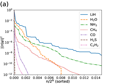
Figure 1: (a) Concentration in the computational basis shown for ground states $\ket{\psi}$ of molecular Hamiltonians listed in Table 1. The distribution of $\absolutevalue{\bra{n}\ket{\psi}}^{2}$ is plotted for $n/2^{N}$, where $\ket{n}$ is a computational basis state and $N$ is the number of qubits. The index $n$ of the computational basis is sorted in descending order of $\absolutevalue{\bra{n}\ket{\psi}}^{2}$. (b) The relative error vs infidelity plot for points corresponding to various $R$ values of different molecular ground states. The relative error $\Delta E=(E_{R}-E_{\mathrm{exact}})/|E_{\mathrm{exact}}|$ is defined for the energy expectations values of the exact ground state $\ket{\psi}$ and truncated state $\ket{\psi_{R}}$ of Eq. (12). The infidelity is given by $1-|\innerproduct{\psi_{R}}{\psi}|^{2}$. See the text for detailed explanation.

We first see whether and how actual ground states of the molecular Hamiltonians are concentrated in the computational basis. Fig. 1(a) shows the distribution of the single-weight factors $\absolutevalue{\bra{n}\ket{\psi}}^{2}$ in the computational basis ($n=0,1,\cdots,2^{N}-1$) sorted in descending order, for each of molecular ground states. The basis index $n$ is normalized by the total number of basis states $2^{N}$ for comparison between molecules of different numbers of qubits $N$. We observe the distributions decay quickly with $n/2^{N}$, implying the ground states are concentrated. Hence we expect only a small fraction of the basis states are relevant in the estimation of the energy expectation values for those molecules.

Next, we investigate the error caused by truncating less-significant computational basis states in the calculation of the expectation value. As explained in the previous section, we retain $R$ most-significant computational basis states by truncating the double sum in the expectation value formula of Eq. (6), and adopt Eq. (13) as an estimator for the expectation value. One must choose a value of $R$ so that the error caused by this truncation is within a required accuracy of the expectation value. Here we present a criterion for this, guided by a formal argument in Appendix C.

As shown in Eq. (29), the difference between expectation values of an observable $O$ for the original state $\ket{\psi}$ and approximate state $\ket{\psi_{R}}$ is bounded by their fidelity:

$$|\expectationvalue{O}{\psi}-\expectationvalue{O}{\psi_{R}}|\leq 2\|O\|_{\infty}\sqrt{1-|\innerproduct{\psi_{R}}{\psi}|^{2}},$$ (21)

where $\|O\|_{\infty}$ is the largest singular value of $O$ and $|\innerproduct{\psi_{R}}{\psi}|^{2}$ is the fidelity between the two states. The fidelity can be expressed as

$$\absolutevalue{\bra{\psi_{R}}\ket{\psi}}^{2}=\sum_{r=1}^{R}\absolutevalue{\bra{z_{r}}\ket{\psi}}^{2},$$ (22)

and hence can be estimated by $1/c_{R}^{2}=\sum_{r=1}^{R}T_{r}/L_{f}$ in our algorithm. This does not require additional measurements. Therefore we are led to take the estimated fidelity $|\innerproduct{\psi}{\psi_{R}}|^{2}$ as a quick indicator to determine $R$.

In the application to the molecular Hamiltonian, our interest is constraining the difference of energy expectation values $E_{\mathrm{exact}}=\expectationvalue{H}{\psi}$ and $E_{R}=\expectationvalue{H}{\psi_{R}}$, for the exact ground state $\ket{\psi}$ and truncated state $\ket{\psi_{R}}$. In Fig. 1(b), the relative error $\Delta E=(E_{R}-E_{\mathrm{exact}})/|E_{\mathrm{exact}}|$ and the infidelity $1-|\innerproduct{\psi_{R}}{\psi}|^{2}$ are plotted for various $R$ values of different molecules. The relative error and infidelity seem positively correlated, and we observe $\Delta E$ is a factor of $0.1$–$0.01$ smaller than the infidelity depending on molecular species. It is notable that this dependence is rather mild. Based on this result, we adopt a constraint on the infidelity as the concrete criterion for determining $R$ in our numerical analysis, which is given as follows: we choose the minimum integer $R^{\prime}$ which satisfies $1-|\innerproduct{\psi_{R^{\prime}}}{\psi}|^{2}\leq 10^{-4}$ as $R$, for all the molecules in our study. In Table 1, the values of $R$ determined by this procedure are shown with the (absolute) truncation error $E_{R}-E_{\rm exact}$. All the molecules exhibit the error smaller than $10^{-3}$ Hartree.

III.3 Comparisons of statistical fluctuations with conventional methods

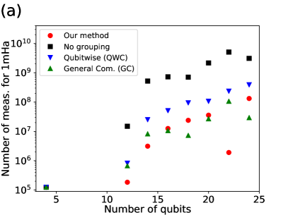
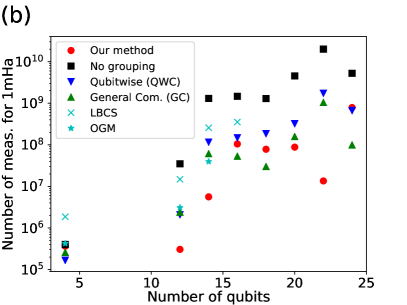
Figure 2: The total number of measurements required to achieve the standard deviation of $10^{-3}$ Hartree in the energy expectation value estimation with the ground state for each of molecules listed in Table 1, based on a different estimation method and measurement allocation strategy. (a) The results based on the measurement allocations optimized for the exact ground states (obtained by FCI calculations). (b) The results based on the heuristic measurement allocations. LBCS and OGM stand for locally-biased classical shadow [30] and overlapped grouping measurement [31], respectively. See the text for detailed explanation.

We estimate statistical fluctuations of expectation values estimated by our method and compare them with those by the other existing methods.

As for our method, we formulate the variances of estimated expectation values in Appendix D.3, where the details can be found. We here consider only the statistical fluctuations caused by finite numbers of measurements $L_{f},\{L_{A_{r}}\}$, and $\{L_{B_{r}}\}$ for $f_{r},A_{r}$ and $B_{r}$, respectively, and do not include any other sources of fluctuations and deviations such as coherent noises in quantum devices. Then, the variance of an expectation value estimated by our method, Eq. (13), can be expressed in terms of the numbers of measurements as

$$\mathrm{Var}[\expectationvalue{O}{\psi}]=\frac{v_{f}}{L_{f}}+\sum_{r=2}^{R}\pqty{\frac{v_{A_{r}}}{L_{A_{r}}}+\frac{v_{B_{r}}}{L_{B_{r}}}},$$ (23)

where the coefficients $v_{f}$, $v_{A_{r}}$ and $v_{B_{r}}$ are defined by Eq. (64). The total number of measurements is

$$L=L_{f}+\sum_{r=2}^{R}\pqty{L_{A_{r}}+L_{B_{r}}}.$$ (24)

We also investigate how to optimally allocate the measurement budget to each of $L_{f},\{L_{A_{r}}\}$, and $\{L_{B_{r}}\}$, when the total number of measurements $L$ is fixed to a certain value. That is, we consider the minimization of the variance (23), under the condition of a fixed $L$. We consider two cases: the first case is when one knows true values of coefficients $v_{f}$, $v_{A_{r}}$ and $v_{B_{r}}$ appearing in the variance formula (23); the second case is when one cannot access those values. In the first case, the optimal allocation of measurements can be achieved and is given by

$$L_{f}:L_{A_{r}}:L_{B_{r}}=\sqrt{v_{f}}:\sqrt{v_{A_{r}}}:\sqrt{v_{B_{r}}},$$ (25)

recasting the variance formula into Eq. (67). In a practical situation where the algorithm is applied to a general state, however, it would be unrealistic to assume values of $v_{f}$, $v_{A_{r}}$ and $v_{B_{r}}$ are known before the measurements are conducted, as those values depend on quantities such as $f_{r}$, $A_{r}$ and $B_{r}$ (see Eq. (64)), which are supposed to be constructed based on the measurement outcomes. Hence, as a more practical case, we also consider the second case.

In the second case, where we are ignorant of values of $v_{f}$, $v_{A_{r}}$ and $v_{B_{r}}$ for a given state, we adopt a heuristic method: we take a reference state for which values of $v_{f}$, $v_{A_{r}}$ and $v_{B_{r}}$ are classically calculated prior to the measurements, and optimize the measurement allocation for this state by Eq. (25); then, we apply the same allocation to arbitrary states considered in the algorithm. In this article, we take the following state as the reference state:

$$\ket{\psi_{w}}=\sqrt{w}\ket{z_{1}}+\sum_{r=2}^{R}\sqrt{\frac{1-w}{R-1}}\ket{z_{r}},$$ (26)

where $w$ is a positive real parameter with $0<w<1$. This is designed as a simplified representative for concentrated states. Using the measurement allocation optimized for $\ket{\psi_{w}}$ with some $w$, we estimate the variance for a given state in the second case (see Eqs. (73) and (74) for explicit formulas). The formulas with detailed derivations are presented in Appendix D.3.

As for the conventional methods, we consider the methods based on the decomposition of an observable into Pauli strings with or without partitioning into co-measurable groups, as briefly described in Sec. II.1. The way of grouping of Pauli strings and the choice of the measurement allocation to each group both affect the variance of the estimated expectation value. We examine combinations of three types of Pauli-string grouping and two types of measurement allocation to each of grouped Pauli strings. For the grouping, we consider (i) no grouping, i.e., all the Pauli strings in an observable are separately measured, (ii) qubit-wise commuting (QWC) grouping, and (iii) general-commuting (GC) grouping. The QWC grouping requires no additional two-qubit gates to simultaneously measure all the Pauli strings in each group [10, 14], while the GC grouping needs extra $\mathcal{O}(N^{2}/\log N)$ two-qubit gates [15, 42] (see also [16, 18]). The details of the three grouping methods are summarized in Appendix E. For the measurement allocation, we again consider the situation where one knows true expectation values of Pauli strings such as $\expectationvalue{P_{i}}{\psi}$ prior to the measurements, and the situation where one cannot access those values without the measurements, just as in our method. The measurement allocation is optimized for the state $\ket{\psi}$ under consideration in the former, while is optimized for Haar random states in the latter. The variances for those two ways of allocation are given by Eqs. (42) and (44), respectively (see Appendix D.2 for details).

Besides the conventional methods, we also consider two recently-proposed methods based on a technique called classical shadow for comparison: one is locally-biased classical shadow (LBCS) [30] and the other is overlapped grouping measurement (OGM) [31]. These methods work without knowing expectation values of observables before measurements and hence are compared with our heuristic method of the measurement allocation. We take the values of the variances presented in Refs. [30, 31] for H2, LiH, H2O (LBCS and OGM) and NH3 (only LBCS).

In Fig. 2, we show the total number of measurements $L$ required to achieve the standard deviation of $10^{-3}$ Hartree, in energy expectation value estimation with the ground state (obtained by the FCI calculation) for each of molecules listed in Table 1, based on a different estimation method and measurement allocation strategy explained above. In Fig. 2(a) the measurement allocations are optimized for the exact ground states in both of the conventional and our methods, while in Fig. 2(b) they are optimized for some reference states, i.e., for the Haar random states in the conventional methods and for the heuristic reference states (Eq. (26)) in our method. As the variances can be parameterized as $c_{v}/L$ for a total number of measurements $L$ with some measurement allocation (see Eq. (35)), one may infer the required $L$ for $10^{-3}$ Hartree by

$$L=\quantity(\frac{\sqrt{c_{v}}}{10^{-3}~{}\ce{Hartree}})^{2},$$ (27)

where $c_{v}$ is a constant defined by Eq. (35) with Eqs. (32) and (34). We take $w=0.75$ in Eq. (26) for our heuristic way of the measurement allocation. In both cases of the measurement allocation strategies, we observe that our method tends to require a smaller number of measurements than two conventional methods, no grouping and QWC grouping. In contrast, the GC grouping tends to compete with our method. Nevertheless, this may still indicate an advantage of our method, given gate complexity of two methods: that is, our method needs $\mathcal{O}(N)$ two-qubit gates while the GC grouping requires $\mathcal{O}(N^{2}/\log N)$ two-qubit gates to estimate an expectation value, in addition to gates for constructing a circuit of the state $\ket{\psi}$ of interest. We note that both of our method and GC grouping tend to demand fewer measurements than the classical-shadow based approaches, LBCS and OGM.

The results in Fig. 2 support the effectiveness of our method in estimating expectation values of molecular Hamiltonians for their ground states.

IV Discussion

We comment on several points in our study before summarizing this article.

IV.1 Potential advantages of our method over conventional methods

Our method performs the summation in Eq. (13), which has $R^{2}$ terms, by classical computers. In general, a value of $R$ that is large enough to approximate the expectation value with sufficient accuracy may be exponentially large in the number of qubits $N$, which will deteriorate the efficiency of our method. The numerical analysis in the previous section demonstrates examples in molecular systems where $R$ can be taken small enough to efficiently process the summation in Eq. (13) with sufficient accuracy retained. Although the scaling of $R$ with $N$ for larger molecules is not known, we expect that values of $R$ do not become so large for ground states of weakly-correlated molecules. In Appendix G, we also investigate the effect of electron correlation by performing the same numerical analysis to the nitrogen molecule N2 for various bond lengths. As N2 is stretched from the equilibrium bond length and the triple bond is broken, the electron correlation is considered to be large, but our method is still more effective than the QWC grouping method. Our numerical results give concrete examples in which our method realizes an actual speedup over the conventional methods in expectation value estimation of observables.

Let us discuss the noise robustness of our method. Since our method picks up dominant computational basis states in the first step of the algorithm, it is easy to mitigate errors of quantum devices that change a symmetry of the computational basis states, by the method called symmetry verification [43, 44, 21]. For example, when we treat an electronic Hamiltonian of some molecule conserving the particle number and employ its qubit representation in which each computational basis state has a definite particle number, e.g., the Jordan-Wigner transformation, the bit-flipping error that changes the count of “1” in the binary representation of the basis state can be easily detected; the ground state must have some fixed particle number, i.e., the number of electrons, and we can simply reject (if any) an observed basis state $\ket{z_{r}}$ that does not have such a particle number. Other types of noises such as dephasing error can be mitigated by the standard techniques of quantum error mitigation [45, 46] in the same manner as the conventional methods.

IV.2 Improvements and extensions of our method

We discuss possible improvements and extensions of our algorithm. First, it may be possible to calculate the interference factors $\bra{m}\ket{\psi}\bra{\psi}\ket{n}$ or $\bra{z_{r}}\ket{\psi}\bra{\psi}\ket{z_{r^{\prime}}}$ in different ways than our explicit algorithm described in Sec. II.2, with lower quantum computational costs. We discuss possible directions in Appendix A. For instance, if $\mathrm{Hamming}(m,n)=1$, where $\mathrm{Hamming}(m,n)$ is the Hamming distance between the binary representations of integers $m$ and $n$, all the interference factors $\bra{m}\ket{\psi}\bra{\psi}\ket{n}$ for possible combinations of arbitrary $m$ and $n$ can be evaluated just based on $2N$ distinct quantum circuits, given the single-weight factors $\absolutevalue{\bra{m}\ket{\psi}}^{2}$ and $\absolutevalue{\bra{n}\ket{\psi}}^{2}$ are already obtained. Each of the quantum circuits only requires an application of the Hadamard (and phase) gates on the state $\ket{\psi}$. Similarly, if $\mathrm{Hamming}(m,n)=2$, all the possible interference factors $\bra{m}\ket{\psi}\bra{\psi}\ket{n}$ can be evaluated just based on $N(N-1)$ distinct quantum circuits, each of which requires a consecutive application of the CNOT and Hadamard (and phase) gates on the state $\ket{\psi}$. These procedures combined with the relation (14) may lead to an improved way to evaluate the interference factors which requires a smaller number of distinct quantum circuits. See Appendix A for details.

Second, in the application to quantum chemistry, fermionic states other than Slater determinants may be identified as the computational basis states, so long as they meet the requirements such as concentration of the state and feasibility of efficient calculation for the transition matrix elements in the basis states. For example, the configuration state functions (CSFs) [47, 48], which preserve the particle number, the total spin, etc., may be identified as the computational basis states, given transition matrix elements between two CSFs can be classically evaluated in $\mathcal{O}(\mathrm{poly}(N))$ time. In the conventional methods to evaluate expectation values, the number of Pauli strings in a Hamiltonian written in such a basis is larger than that written in a basis of Slater determinants and it becomes more costly to evaluate the expectation value. On the other hand, in our method, putting more focus on a quantum state, the expectation value will be evaluated efficiently as long as the state is concentrated.

IV.3 Relationship to classical computational methods

Finally, we would like to discuss relationship between our algorithm and classical computational methods in quantum chemistry. Performing the importance sampling for Eq. (6) is considered in the variational Monte Carlo (VMC) [49, 50], although the summations for $m$ and $n$ are separately done. Compared to VMC, our approach uses quantum computers and we can, in principle, use an arbitrary unitary quantum circuit $U$ to generate a general quantum state $\ket{\psi}=U\ket{0}$ on qubits. On the other hand, in VMC, a quantum state is supposed to have a property that complex amplitudes $\innerproduct{n}{\psi}$ are efficiently calculable on classical computers. For example, when the unitary coupled-cluster ansatz [51] is employed for $U$, it is suggested that classical computation of $\innerproduct{n}{\psi}$ is hard [52]. In that case, we may potentially have a quantum advantage in the sense that we can use wavefunctions that are difficult to be used with VMC. We also analyze variances of expectation values obtained by the importance sampling of Eq. (6) in the same manner as VMC in Appendix H.

Other related classical computational methods are the adaptive-sampling configuration interaction (ASCI) and similar methods [53, 54, 55, 56, 57], where important basis states to represent the ground state of a given Hamiltonian $H$ are adaptively chosen and the exact diagonalization within the selected basis states is iteratively performed. From the viewpoint of searching for important basis states, our algorithm automatically picks up such basis states by projective measurements on a quantum state $\ket{\psi}$ if $\ket{\psi}$ is concentrated in the basis states, whereas ASCI relies on state-of-the-art techniques in classical computation [57] to search through a large number (possibly exponential in $N$) of basis states. Note that our algorithm described in this article focuses on the evaluation of just the expectation value $\expectationvalue{H}{\psi}$ for a given state $\ket{\psi}$, and cannot be compared on the same footing with ASCI which performs the exact diagonalization of $H$.

V Summary

In this study, we proposed a hybrid quantum-classical algorithm to efficiently measure expectation values of observables for quantum states concentrated in a measurement basis. Taking the computational basis with $\ket{n}$ ($n=0,1,\cdots,2^{N}-1$) as the measurement basis, we first rewrote the expectation value $\expectationvalue{O}{\psi}$ of an observable $O$ for a state $\ket{\psi}$ by expanding the state in terms of the computational basis states. This resulted in a weighted sum of transition matrix elements $\matrixelement{m}{O}{n}$ with interference factors $\bra{m}\ket{\psi}\bra{\psi}\ket{n}$. We then approximated the sum with a limited number of computational basis states based on the empirical insight that quantum states in which we are interested are often concentrated: for example, in quantum chemistry, only a small number of Slater determinants such as the Hartree-Fock state are sufficient to describe low-lying electronic energy eigenstates for weakly-correlated molecules; though our method is applicable beyond the weak correlation.

We gave explicit procedures to measure and calculate the ingredients appearing in the truncated summation. The single weight factors $|\innerproduct{n}{\psi}|^{2}$ and the normalization factor are estimated by projective measurement for $\ket{\psi}$ in the computational basis, while the transition matrix elements $\matrixelement{m}{O}{n}$ are efficiently calculated by classical computation. The interference factors $\bra{m}\ket{\psi}\bra{\psi}\ket{n}$ are estimated by projective measurements of some states in the computational basis, where each of the states is realized by an appropriate unitary transformation, consisting of at most $N$ CNOT gates, applied to $\ket{\psi}$. In our method, the number of quantities measured on quantum computers depends on the quantum state instead of the observable. This contrasts with the conventional methods of expectation value estimation, where the observable is expanded into a plethora of Pauli strings that are separately measured on quantum computers.

For a quantitative comparison, we numerically estimated variances for estimated expectation values of Hamiltonians for electronic states of small molecules, i.e., energy expectation values. We derived formulas to calculate the variances of expectation values estimated by our method. We employed the exact ground states to estimate the variances of the energy expectation values and inferred the total numbers of measurements to achieve the standard deviation of $10^{-3}$ Hartree, which is comparable to the so-called chemical accuracy in quantum chemistry. The numerical results illustrate that our approach can outperform the conventional methods to estimate the expectation values.

As a future work, combining our method with VQE, e.g., as a subroutine to estimate expectation values, would be interesting not only for accelerating VQE, but also for envisioning how our proposal can contribute to various variational quantum algorithms. In the numerical analysis, we used exact ground states of Hamiltonians for estimating the variances because our focus was to illustrate the performance in a single evaluation of expectation values. In application to VQE, the estimation of expectation values is needed during the optimization procedure and hence a target quantum state may not be well concentrated, especially at initial steps of the optimization. In such a case, the summation in our expectation value formula would require the inclusion of many basis states, possibly spoiling the effectiveness of our algorithm. Although we focused on the application to quantum chemistry for demonstrating effectiveness of our algorithm, the algorithm is open to general applications that rely on expectation value estimation.

Appendix A Alternative ways to estimate interference factors

We gave an explicit algorithm to calculate the interference factors $\bra{m}\ket{\psi}\bra{\psi}\ket{n}$ or $\bra{z_{r}}\ket{\psi}\bra{\psi}\ket{z_{r^{\prime}}}$ in Sec. II.2. It was meant just for illustration, and it may be possible to calculate them in different ways hopefully with lower quantum computational costs.

For example, suppose the Hadamard gate is applied on the first qubit ($\mathrm{Had}_{1}$) of a state $\ket{\psi}$ and the projective measurement is performed for the overall state in the computational basis. By this measurement, one can estimate the probabilities with which each of all the $N$-bit strings, from “$0\cdots 0$” to “$1\cdots 1$”, appears. When $N=4$, for instance, the probability for “0011” is written as $|\matrixelement{0011}{\mathrm{Had}_{1}}{\psi}|^{2}=|\frac{1}{\sqrt{2}}(\bra{0011}+\bra{1011})\ket{\psi}|^{2}$, contributing to the $\mathcal{A}$ term (see Eq. (8) for definition) of the interference factor $\bra{0011}\ket{\psi}\bra{\psi}\ket{1011}$; the probability for “0101” is $|\matrixelement{0101}{\mathrm{Had}_{1}}{\psi}|^{2}=|\frac{1}{\sqrt{2}}(\bra{0101}+\bra{1101})\ket{\psi}|^{2}$, contributing to the $\mathcal{A}$ term of $\bra{0101}\ket{\psi}\bra{\psi}\ket{1101}$. This example indicates that one can evaluate all the $2^{N-1}$ possible $\mathcal{A}$ terms consisting of $\ket{0b_{2}\cdots b_{N}}$ and $\ket{1b_{2}\cdots b_{N}}$ ($b_{2},\cdots,b_{N}=0,1$), solely based on a single quantum circuit. The $\mathcal{B}$ term counterparts can be similarly evaluated but by measuring the state ${\mathrm{Had}_{1}}S_{1}\ket{\psi}$, augmented by the phase gate on the first qubit $S_{1}={\rm diag}(1,i)$. Then, all the corresponding interference factors can be obtained via Eq. (8), with the single-weight factors evaluated by measuring the state $\ket{\psi}$. This procedure combined with the relation (14) may lead to an improved way to evaluate the interference factors which requires a smaller number of distinct quantum circuits.

We remind that, in the application to electronic structure problems with the Jordan-Wigner mapping, the above procedure gives interference factors between electronic states of different electron numbers and would not be useful in settings where the electron number is conserved. Yet, even in such a case, similar procedures may still work to evaluate interference factors between electronic states of an equal electron number based on the parity mapping or Bravyi-Kitaev mapping [58] for encoding fermionic states onto qubits. Or, keeping the Jordan-Wigner mapping, one can consecutively apply the CNOT and Hadamard (and phase) gates on the state $\ket{\psi}$ to obtain $\mathcal{A}$ ($\mathcal{B}$) terms with $\ket{01b_{3}\cdots b_{N}}$ and $\ket{10b_{3}\cdots b_{N}}$, both having a same electron number. In line with these ideas, our algorithm may be better implemented with lower computational costs.

Appendix B Detail of numerical analysis

The geometries of molecules used in Sec. III are summarized in Table 2.

Table 2: Geometries of molecules. “$(\mathrm{X},(x,y,z))$” denotes three dimensional coordinates $x,y,z$ of atom X in units of Å.

Molecule	Geometry
H2	(H, (0, 0, 0)), (H, (0, 0, 0.735))
LiH	(Li, (0, 0, 0)), (H, (0, 0, 1.548))
H2O	(O, (0, 0, 0.137)), (H, (0,0.769,-0.546)), (H, (0,-0.769,-0.546))
NH3	(N, (0,0,0.149)), (H, (0,0.947,-0.348)), (H, (0.821,-0.474,-0.348)), (H, (-0.821,-0.474,-0.348))
CH4	(C, (0, 0, 0)), (H, (0.6276, 0.6276, 0.6276)), (H, (0.6276, -0.6276, -0.6276)),
	(H, (-0.6276, 0.6276, -0.6276)), (H, (-0.6276, -0.6276, 0.6276))
CO	(C, (0, 0, 0)), (O, (0, 0, 1.128))
H2S	(S, (0, 0, 0.1030)), (H, (0, 0.9616, -0.8239)), (H, (0, -0.9616, -0.8239))
C2H2	(C, (0, 0, 0.6013)), (C, (0, 0, -0.6013)), (H, (0, 0, 1.6644)), (H, (0, 0, -1.6644))

Appendix C Approximating wavefunctions and expectation values

In this section, we prove Eq. (21) in the main text.

Let us consider two quantum states (density matrices) $\rho,\sigma$ and an observable $O$ which is written as $O=\sum_{i}o_{i}E_{i}$ by the spectral decomposition (i.e., $o_{i}\in\mathbb{R}$ is an eigenvalue and $E_{i}$ is the corresponding projector). We can bound the difference of expectation values of $O$ with respect to $\rho$ and $\sigma$ as

$$\Tr((\rho-\sigma)O) =\sum_{i}o_{i}\Tr((\rho-\sigma)E_{i})$$

$$\leq\sum_{i}|o_{i}||\Tr((\rho-\sigma)E_{i})|$$

$$\leq\|O\|_{\infty}\sum_{i}\Tr(|\rho-\sigma|E_{i})$$

$$=2\|O\|_{\infty}D(\rho,\sigma),$$

where $\|O\|_{\infty}$ is the infinite norm (the largest singular value) of $O$ and $D(\rho,\sigma)=\Tr(|\rho-\sigma|)/2$ is the trace distance. We have used an inequality $|\Tr((\rho-\sigma)E_{i})|\leq\Tr(|\rho-\sigma|E_{i})$ (see Section 9.2 of [33]) and the completeness relation of the projectors $\sum_{i}E_{i}=I$. When two states are both pure, i.e., $\rho=\ket{\psi}\!\bra{\psi}$ and $\sigma=\ket{\phi}\!\bra{\phi}$, the trace distance is expressed by the fidelity $|\innerproduct{\psi}{\phi}|^{2}$:

$$D(\rho,\sigma)=\sqrt{1-|\innerproduct{\psi}{\phi}|^{2}}.$$ (28)

Therefore, when we approximate an original quantum state $\ket{\psi}$ by the truncated state $\ket{\psi_{R}}$, the difference of expectation values is bounded by their infidelity:

$$|\expectationvalue{O}{\psi}-\expectationvalue{O}{\psi_{R}}|\leq 2\|O\|_{\infty}\sqrt{1-|\innerproduct{\psi}{\psi_{R}}|^{2}}.$$ (29)

Appendix D Variance formulas

In this section, we first review the formulas for variances of estimated expectation values of an observable $O$ with a given state $\ket{\psi}$ in the conventional methods based on the decomposition of $O$ into Pauli strings. We also present the ways how to (near) optimally allocate the measurement budget to each of quantities measured in the estimation procedures in the view of minimizing the variance, depending on whether one can access the values of the quantities to be measured prior to the measurements or not. Then, we show the formulas for variances of estimated expectation values in our method. The (near) optimal allocations of measurements to minimize the variance are also considered for the same situations as the conventional methods.

D.1 General formulas for optimal allocation of measurement budget

Both in the conventional and our methods, the variance of an expectation value can be written as

$$\mathrm{Var}[\expectationvalue{O}{\psi}]=\sum_{\lambda}\frac{v_{\lambda}}{L_{\lambda}},$$ (30)

where $L_{\lambda}$ is the number of measurements to evaluate some quantity labeled by $\lambda$ and $v_{\lambda}$ is the variance per single measurement for that quantity. Minimizing the variance under the constraint of a fixed total number of measurements, $\sum_{\lambda}L_{\lambda}=L$, one obtains the optimal number of measurements for each $\lambda$ given by [25, 26, 27]

$$L_{\lambda}=L\frac{\sqrt{v_{\lambda}}}{\sum_{\lambda^{\prime}}\sqrt{v_{\lambda^{\prime}}}}.$$ (31)

Plugging this into Eq. (30) gives the variance for the optimal allocation of the measurement budget:

$$\quantity(\mathrm{Var}[\expectationvalue{O}{\psi}])^{*}=\frac{\quantity(\sum_{\lambda}\sqrt{v_{\lambda}})^{2}}{L}.$$ (32)

This derivation tacitly assumes one can access the values of $v_{\lambda}$ for the state $\ket{\psi}$ of interest prior to the measurements, which would be, however, unrealistic in practical situations. When those values are unknown, one can still make a heuristic guess for the measurement allocation to reduce the variance. That is, one introduces a reference state $\ket{\psi^{\rm ref}}$ for which the values of $v_{\lambda}^{\rm ref}$ in Eq. (30) can be obtained by classical computation, and then optimizes the measurement allocation with respect to this state:

$$L_{\lambda}=L\frac{\sqrt{v_{\lambda}^{\rm ref}}}{\sum_{\lambda^{\prime}}\sqrt{v^{\rm ref}_{\lambda^{\prime}}}}.$$ (33)

With this measurement allocation, the variance for the state $\ket{\psi}$ of interest becomes

$$\quantity(\mathrm{Var}[\expectationvalue{O}{\psi}])^{\rm ref}=\frac{1}{L}\quantity(\sum_{\lambda}\sqrt{v_{\lambda}^{\rm ref}})\quantity(\sum_{\lambda}\frac{v_{\lambda}}{\sqrt{v_{\lambda}^{\rm ref}}}).$$ (34)

Both in the conventional and our methods for both ways of the measurement allocation, the variance as a function of the total number of measurements $L$ can be written as

$$\quantity(\mathrm{Var}[\expectationvalue{O}{\psi}])^{\rm opt}=\frac{c_{v}}{L},$$ (35)

where $c_{v}$ is a constant consisting of $v_{\lambda}$ and/or $v_{\lambda}^{\rm ref}$ (see Eqs. (32) and (34) for the definition). We will use these general formulas when deriving the optimal allocation of measurements in the following.

D.2 Conventional methods based on grouping of Pauli strings

The conventional methods for expectation value estimation utilize the expansion of the target observable $O$ by Pauli strings $P_{i}$, given in Eq. (2):

$$O=\sum_{i=1}^{M}c_{i}P_{i},$$ (36)

where $c_{i}$ are real coefficients, and $M$ is the number of the Pauli strings. Moreover, to save the measurement budget, one can divide Pauli strings into several groups where all Pauli strings in each group can be measured simultaneously:

$$O =\sum_{g}O_{g},$$ (37)

$$O_{g} =\sum_{k=1}^{M_{g}}c_{k}^{(g)}P_{k}^{(g)}.$$ (38)

In this expression, $g$ labels the groups; $c_{k}^{(g)}$ and $P_{k}^{(g)}$ are coefficients and Pauli strings in a group $g$, respectively; $M_{g}$ is the number of Pauli strings in a group $g$. The ability to perform the simultaneous measurement is assured by imposing the condition $[P_{k}^{(g)},P_{k^{\prime}}^{(g)}]=P_{k}^{(g)}P_{k^{\prime}}^{(g)}-P_{k^{\prime}}^{(g)}P_{k}^{(g)}=0$ in grouping, for any pair of $k,k^{\prime}$ within a group $g$. How to group Pauli strings in the original observable [Eq. (36)] is explained in Appendix E.

The expectation value and the (single-measurement) variance for $O_{g}$ are given by

$$\mathrm{Exp}[O_{g}] =\expectationvalue{O_{g}}{\psi},$$ (39)

$$\mathrm{Var}[O_{g}] =\expectationvalue{O_{g}^{2}}{\psi}-\expectationvalue{O_{g}}{\psi}^{2},$$ (40)

respectively. When one performs $L_{g}$ times of measurements for each group $g$, the variance for the overall expectation value $\expectationvalue{O}{\psi}$ is given by

$$\mathrm{Var}[\expectationvalue{O}{\psi}]_{\mathrm{grouping}}=\sum_{g}\frac{\mathrm{Var}[O_{g}]}{L_{g}},$$ (41)

because measurements for different groups are independent.

When one can access the value of $\mathrm{Var}[O_{g}]$, or $\expectationvalue{O_{g}}{\psi}$ and $\expectationvalue{O_{g}^{2}}{\psi}$, it is possible to optimize the number of measurements $L_{g}$ for each group $g$ by using Eq. (31) and the minimal variance under the constraint $\sum_{g}L_{g}=L$ is obtained as

$$\quantity(\mathrm{Var}[\expectationvalue{O}{\psi}]_{\mathrm{grouping}})^{*} =\frac{1}{L}\quantity(\sum_{g}\sqrt{\mathrm{Var}[O_{g}]})^{2}$$

$$=\frac{1}{L}\quantity(\sum_{g}\sqrt{\sum_{k,k^{\prime}}c_{k}^{(g)}c_{k^{\prime}}^{(g)}\quantity(\expectationvalue{P_{k}^{(g)}P_{k^{\prime}}^{(g)}}{\psi}-\expectationvalue{P_{k}^{(g)}}{\psi}\!\expectationvalue{P_{k^{\prime}}^{(g)}}{\psi})})^{2},$$ (42)

according to Eq. (32). However, in most practical cases, one does not know the values for $\expectationvalue{O_{g}^{2}}{\psi}$ and $\expectationvalue{O_{g}}{\psi}$. In such cases, the optimal numbers of measurements can be heuristically guessed by using expectation values for Haar random states [25, 16]. The expectation values for Haar random state satisfy $\expectationvalue{P_{i}}_{\mathrm{Haar}}=0$ for any Pauli string $P_{i}$, and the guessed variance is

$$\mathrm{Var}[O_{g}]^{\mathrm{Haar}}=\sum_{k}(c_{k}^{(g)})^{2}.$$ (43)

By employing the numbers of measurements Eq. (31) for these variances and putting them into Eq. (30), the resulting variance for this heuristic choice of the numbers of measurements is

$$\quantity(\mathrm{Var}[\expectationvalue{O}{\psi}]_{\mathrm{grouping}})^{\mathrm{Haar}}$$

$$=\frac{1}{L}\quantity(\sum_{g}\frac{\mathrm{Var}[O_{g}]}{\sqrt{\mathrm{Var}[O_{g}]^{\mathrm{Haar}}}})\quantity(\sum_{g}\sqrt{\mathrm{Var}[O_{g}]^{\mathrm{Haar}}}).$$ (44)

This corresponds to the general formula of Eq. (34). Here we adopt the Haar random state to decide the measurement allocation in part because of its simplicity, but the use of other classically tractable states, e.g., the state obtained by CISD method, is also possible [8]. The latter could in principle reduce the variance of the expectation value for some state of interest, but this is beyond the scope of this work.

D.3 Our method

Here we give the formulas for the variance of the expectation value $\expectationvalue{O}{\psi}$ in our method as well as the (near) optimal allocation of the measurement budget to minimize the variance of the estimated expectation value.

D.3.1 Variance of $\expectationvalue{O}{\psi}$

We estimate the expectation value by the algorithm described in Sec. II.2. The expectation value is approximated as

$$\expectationvalue{O}{\psi}\approx{\mathcal{N}_{R}}^{2}\sum_{r,r^{\prime}=1}^{R}|\innerproduct{z_{r}}{\psi}|^{2}|\innerproduct{z_{r^{\prime}}}{\psi}|^{2}\frac{\matrixelement{z_{r}}{O}{z_{r^{\prime}}}}{\innerproduct{z_{r}}{\psi}\innerproduct{\psi}{z_{r^{\prime}}}},$$ (45)

which is evaluated by the measured quantities $f_{r},c_{R},A_{r}$, and $B_{r}$:

$$|\innerproduct{z_{r}}{\psi}|^{2} \simeq f_{r},$$ (46)

$$\mathcal{N}_{R} \simeq c_{R},$$ (47)

$$\bra{z_{1}}\ket{\psi}\bra{\psi}\ket{z_{r}} \simeq g_{r}\quad(r=2,\cdots,R),$$ (48)

$$\bra{z_{r}}\ket{\psi}\bra{\psi}\ket{z_{1}} \simeq g_{r}^{*}\quad(r=2,\cdots,R),$$ (49)

$$\bra{z_{r}}\ket{\psi}\bra{\psi}\ket{z_{r^{\prime}}} \simeq\frac{g_{r}^{*}g_{r^{\prime}}}{f_{1}}\>(r\neq r^{\prime}\text{and}\>r,r^{\prime}=2,\cdots,R),$$ (50)

with

$$g_{r}=A_{r}+iB_{r}-\frac{1+i}{2}(f_{1}+f_{r}).$$ (51)

In the following derivation of the variance formula, we omit the effect of normalization, $\mathcal{N}_{R}$, to ease the analysis of the variance. More precisely, we approximate $\ket{\psi}$ by $\ket{\psi_{R}}$ and set $\mathcal{N}_{R}=1$ throughout in this subsection. Numerical results in Sec. III.3 are computed under this assumption. Since we consider $\mathcal{N}_{R}\approx 1-10^{-4}$ in our study, the error in the variance estimations caused by this approximation will be small and we believe it does not affect the conclusion in Sec. III.3. This point is explicitly examined in Appendix F and we find the error is small.

The expectation value $\expectationvalue{O}{\psi}$ depends on measured quantities $\{f_{r}\}_{r=1}^{R},\{A_{r}\}_{r=2}^{R}$, and $\{B_{r}\}_{r=2}^{R}$. The variance of $\expectationvalue{O}{\psi}$ is given by the error propagation formula as

$$\mathrm{Var}[\expectationvalue{O}{\psi}]_{\text{our method}}$$

$$=\sum_{r=1}^{R}\sum_{r^{\prime}=1}^{R}\frac{\partial\expectationvalue{O}}{\partial f_{r}}\frac{\partial\expectationvalue{O}}{\partial f_{r^{\prime}}}{\rm Cov}[f_{r},f_{r^{\prime}}]$$

$$\quad+\sum_{r=2}^{R}\left(\frac{\partial\expectationvalue{O}}{\partial A_{r}}\right)^{2}{\rm Var}[A_{r}]+\sum_{r=2}^{R}\left(\frac{\partial\expectationvalue{O}}{\partial B_{r}}\right)^{2}{\rm Var}[B_{r}],$$ (52)

where we denote $\expectationvalue{O}=\expectationvalue{O}{\psi}$ and the derivatives are explicitly given by

$$\frac{\partial\expectationvalue{O}}{\partial f_{1}}$$

$$=\matrixelement{z_{1}}{O}{z_{1}}+2{\rm Re}\sum_{r=2}^{R}\frac{f_{r}}{g_{r}}\left[1+\left(\frac{1+i}{2}\right)\frac{f_{1}}{g_{r}}\right]\matrixelement{z_{1}}{O}{z_{r}}$$

$$\quad+2{\rm Re}\sum_{r=2}^{R}\sum_{r^{\prime}=r+1}^{R}\frac{f_{r}f_{r^{\prime}}}{g_{r}^{*}g_{r^{\prime}}}$$

$$\quad\times\left[1+\left(\frac{1+i}{2}\right)\frac{f_{1}}{g_{r^{\prime}}}+\left(\frac{1-i}{2}\right)\frac{f_{1}}{g_{r}^{*}}\right]\matrixelement{z_{r}}{O}{z_{r^{\prime}}},$$ (53)

and

$$\frac{\partial\expectationvalue{O}}{\partial f_{r}}$$

$$=\matrixelement{z_{r}}{O}{z_{r}}+2{\rm Re}\frac{f_{1}}{g_{r}}\left[1+\left(\frac{1+i}{2}\right)\frac{f_{r}}{g_{r}}\right]\matrixelement{z_{1}}{O}{z_{r}}$$

$$\quad+2{\rm Re}\sum_{r^{\prime}\geq 2,\neq r}\frac{f_{1}f_{r^{\prime}}}{g_{r}^{*}g_{r^{\prime}}}\left[1+\left(\frac{1-i}{2}\right)\frac{f_{r}}{g_{r}^{*}}\right]\matrixelement{z_{r}}{O}{z_{r^{\prime}}},$$ (54)

$$\frac{\partial\expectationvalue{O}}{\partial A_{r}}$$

$$=-2{\rm Re}\frac{f_{1}f_{r}}{g_{r}^{2}}\pqty{\matrixelement{z_{1}}{O}{z_{r}}+\sum_{r^{\prime}\geq 2,\neq r}\frac{f_{r^{\prime}}}{g_{r^{\prime}}^{*}}\matrixelement{z_{r^{\prime}}}{O}{z_{r}}},$$ (55)

$$\frac{\partial\expectationvalue{O}}{\partial B_{r}}$$

$$=2{\rm Im}\frac{f_{1}f_{r}}{g_{r}^{2}}\pqty{\matrixelement{z_{1}}{O}{z_{r}}+\sum_{r^{\prime}\geq 2,\neq r}\frac{f_{r^{\prime}}}{g_{r^{\prime}}^{*}}\matrixelement{z_{r^{\prime}}}{O}{z_{r}}},$$ (56)

for $r=2,\cdots,R$, and $\mathrm{Cov}[f_{r},f_{r^{\prime}}],\mathrm{Var}[A_{r}]$, and $\mathrm{Var}[B_{r}]$ represent the covariance between $f_{r}$ and $f_{r^{\prime}}$, the variance of $A_{r}$, and the variance of $B_{r}$, respectively. Note that we evaluate all $f_{1},\cdots,f_{R}$ at the same time (in one experiment) and the covariance between $f_{r}$ and $f_{r^{\prime}}$ is non-zero.

As described in Sec. II, the values of measured $f_{1},\cdots,f_{R}$ are evaluated by the numbers of occurrence of the result $z_{1},\cdots,z_{R}$ in the projective measurement for $\ket{\psi}$ which is repeated $L_{f}$ times. The numbers of the occurrence $T_{1},\cdots,T_{R}$ obey the multinomial distribution, and the variance and covariance are given by

$$\mathrm{Var}[T_{r}] =L_{f}p_{r}(1-p_{r}),$$ (57)

$$\mathrm{Cov}[T_{r},T_{r^{\prime}}] =-L_{f}p_{r}p_{r^{\prime}}\quad(r\neq r^{\prime}),$$ (58)

where $p_{r}=|\innerproduct{z_{r}}{\psi}|^{2}$ is the probability for measuring $z_{r}$ (note that only $z_{1},\cdots,z_{R}$ are observed since we approximate $\ket{\psi}$ by $\ket{\psi_{R}}$). Since $f_{r}=T_{r}/L_{f}$, we reach

$$\mathrm{Var}[f_{r}] =\frac{f_{r}(1-f_{r})}{L_{f}}\quad(r=1,\cdots,R),$$ (59)

$$\mathrm{Cov}[f_{r},f_{r^{\prime}}] =-\frac{f_{r}f_{r^{\prime}}}{L_{f}}\quad(r\neq r^{\prime}).$$ (60)

We define $\mathrm{Cov}[f_{r},f_{r}]=\mathrm{Var}[f_{r}]$ for simplifying the notation. On the other hand, $A_{r}$ ($r=2,\cdots,R$) is measured as a frequency of obtaining the result “0” when measuring a state $U_{z_{1},z_{r}}\ket{\psi}$ in the computational basis. Since we repeat the measurement $L_{A_{r}}$ times for each $r$, the variance of $A_{r}$ is given by a simple binomial distribution of the probability $|\matrixelement{0}{U_{z_{1},z_{r}}}{\psi}|^{2}\simeq A_{r}$:

$$\mathrm{Var}[A_{r}]=\frac{A_{r}(1-A_{r})}{L_{A_{r}}},$$ (61)

for $r=2,\cdots,R$. Similarly, the variance of $B_{r}$ for $L_{B_{r}}$ measurements is given by

$$\mathrm{Var}[B_{r}]=\frac{B_{r}(1-B_{r})}{L_{B_{r}}},$$ (62)

for $r=2,\cdots,R$.

By putting Eqs. (59)-(62) into Eq. (52), we eventually reach the formula in the form of Eq. (30):

$$\mathrm{Var}[\expectationvalue{O}{\psi}]_{\text{our method}}=\frac{v_{f}}{L_{f}}+\sum_{r=2}^{R}\pqty{\frac{v_{A_{r}}}{L_{A_{r}}}+\frac{v_{B_{r}}}{L_{B_{r}}}},$$ (63)

where

$$v_{f} =\sum_{r=1}^{R}\left(\frac{\partial\expectationvalue{O}}{\partial f_{r}}\right)^{2}f_{r}(1-f_{r})-\sum_{r\neq r^{\prime}}\frac{\partial\expectationvalue{O}}{\partial f_{r}}\frac{\partial\expectationvalue{O}}{\partial f_{r^{\prime}}}f_{r}f_{r^{\prime}},$$

$$v_{A_{r}} =\left(\frac{\partial\expectationvalue{O}}{\partial A_{r}}\right)^{2}A_{r}(1-A_{r}),$$

$$v_{B_{r}} =\left(\frac{\partial\expectationvalue{O}}{\partial B_{r}}\right)^{2}B_{r}(1-B_{r}).$$ (64)

D.3.2 Optimal allocation of measurement budget

We discuss the optimization of the numbers of measurements $L_{f},\{L_{A_{r}}\}_{r=2}^{R},\{L_{B_{r}}\}_{r=2}^{R}$ to minimize the variance (63). We fix the total number of measurements:

$$L=L_{f}+\sum_{r=2}^{R}\pqty{L_{A_{r}}+L_{B_{r}}}.$$ (65)

We again consider the situation where one can use information of values for $f_{r},A_{r},B_{r}$, or the situation where one cannot.

When the values can be used, by the results in Sec. D.1, the optimal numbers of measurements are

$$L_{f}=L\sqrt{\frac{v_{f}}{v}},~{}L_{A_{r}}=L\sqrt{\frac{v_{A_{r}}}{v}},~{}L_{B_{r}}=L\sqrt{\frac{v_{B_{r}}}{v}},$$ (66)

where $\sqrt{v}=\sqrt{v_{f}}+\sum_{r=2}^{R}\pqty{\sqrt{v_{A_{r}}}+\sqrt{v_{B_{r}}}}$. The minimal variance achieved by those numbers of measurements is

$$\quantity(\mathrm{Var}[\expectationvalue{O}{\psi}]_{\text{our method}})^{*}$$

$$=\frac{1}{L}\pqty{\sqrt{v_{f}}+\sum_{r=2}^{R}\pqty{\sqrt{v_{A_{r}}}+\sqrt{v_{B_{r}}}}}^{2}.$$ (67)

When one cannot utilize the values of $f_{r},A_{r},B_{r}$ prior to the measurements, we propose using the following heuristic wavefunction,

$$\ket{\psi_{w}}=\sqrt{w}\ket{z_{1}}+\sum_{r=2}^{R}\sqrt{\frac{1-w}{R-1}}\ket{z_{r}},$$ (68)

where $w$ is a real parameter in $0<w<1$, set by hand. This state mimics a quantum state concentrating especially on $\ket{z_{1}}$ with a (large) weight $w$ and having equal weights for the other computational basis states $\ket{z_{2}},\cdots,\ket{z_{R}}$. For the ground states of molecular Hamiltonians, the Hartree-Fock states (mean-field solutions of the Hamiltonians) typically have large overlaps with the exact ground states; so the use of the heuristic state $\ket{\psi_{w}}$ might be helpful to guess the variances of $f_{r},A_{r},B_{r}$ and to choose the numbers of measurements leading to a relatively small variance of the expectation value $\expectationvalue{O}{\psi}$. We use the values of $f_{r},A_{r},B_{r}$ for this state,

$$f_{1}^{w} =w,\quad f_{2}^{w}=\cdots=f_{R}^{w}=\frac{1-w}{R-1},$$ (69)

$$A_{2}^{w} =\cdots=A_{R}^{w}=\frac{1}{2}\absolutevalue{\sqrt{w}+\sqrt{\frac{1-w}{R-1}}}^{2},$$ (70)

$$B_{2}^{w} =\cdots=B_{R}^{w}=\frac{1}{2}\absolutevalue{\sqrt{w}+i\sqrt{\frac{1-w}{R-1}}}^{2},$$ (71)

and guess the coefficients in Eq. (63) as

$$v_{f}^{w} =\sum_{r=1}^{R}\left.\quantity(\partialderivative{\expectationvalue{O}}{f_{r}})^{2}\right|_{\ket{\psi_{w}}}f_{r}^{w}(1-f_{r}^{w})$$

$$-\sum_{r\neq r^{\prime}}\left.\partialderivative{\expectationvalue{O}}{f_{r}}\right|_{\ket{\psi_{w}}}\left.\partialderivative{\expectationvalue{O}}{f_{r^{\prime}}}\right|_{\ket{\psi_{w}}}f_{r}^{w}f_{r^{\prime}}^{w},$$

$$v_{A_{r}}^{w} =\left.\left(\frac{\partial\expectationvalue{O}}{\partial A_{r}}\right)^{2}\right|_{\ket{\psi_{w}}}A_{r}^{w}(1-A_{r}^{w}),$$

$$v_{B_{r}}^{w} =\left.\left(\frac{\partial\expectationvalue{O}}{\partial B_{r}}\right)^{2}\right|_{\ket{\psi_{w}}}B_{r}^{w}(1-B_{r}^{w}),$$ (72)

where $\left.\partialderivative{\expectationvalue{O}}{f_{r}}\right|_{\ket{\psi_{w}}},\left.\partialderivative{\expectationvalue{O}}{A_{r}}\right|_{\ket{\psi_{w}}},\left.\partialderivative{\expectationvalue{O}}{B_{r}}\right|_{\ket{\psi_{w}}}$ mean that we use $f_{r}^{w},A_{r}^{w}$, and $B_{r}^{w}$ in the formulas Eqs. (53)-(56). We decide the measurement allocation for the state $\ket{\psi}$, with which the expectation value is estimated, based on these guessed variances,

$$L_{f}^{w}=L\sqrt{\frac{v_{f}^{w}}{v^{w}}},~{}L_{A_{r}}^{w}=L\sqrt{\frac{v_{A_{r}}^{w}}{v^{w}}}~{},L_{B_{r}}^{w}=L\sqrt{\frac{v_{B_{r}}^{w}}{v^{w}}},$$ (73)

where $\sqrt{v^{w}}=\sqrt{v_{f}^{w}}+\sum_{r=2}^{R}\pqty{\sqrt{v_{A_{r}}^{w}}+\sqrt{v_{B_{r}}^{w}}}$. The variance with this measurement allocation is

$$\quantity(\mathrm{Var}[\expectationvalue{O}{\psi}]_{\text{our method}})^{w}$$

$$=\frac{1}{L}\pqty{\sqrt{v_{f}^{w}}+\sum_{r=2}^{R}\pqty{\sqrt{v_{A_{r}}^{w}}+\sqrt{v_{B_{r}}^{w}}}}$$

$$\quad\times\pqty{\frac{v_{f}}{\sqrt{v_{f}^{w}}}+\sum_{r=2}^{R}\pqty{\frac{v_{A_{r}}}{\sqrt{v_{A_{r}}^{w}}}+\frac{v_{B_{r}}}{\sqrt{v_{B_{r}}^{w}}}}}.$$ (74)

This corresponds to the general formula of Eq. (34).

Appendix E Grouping of Pauli strings

In this section, we review algorithms to divide Pauli strings contained in an observable into simultaneously-measurable groups, which are used in numerical analysis in Sec. III to estimate the variances of the conventional methods.

As explained in the main text and Appendix  D.2, the grouping of Pauli strings appearing in a Hamiltonian can reduce the variance of the estimated expectation value [18]. We define two types of commutability among Pauli strings $P=\otimes_{s=1}^{N}P^{[s]}$, where $P^{[s]}\in\{I,X,Y,Z\}$ is the Pauli operator acting on a qubit $s=1,\cdots,N$: one type is qubit-wise commuting [10, 14] and the other is generally commuting. Two Pauli strings $P=\otimes_{s=1}^{N}P^{[s]}$ and $Q=\otimes_{s=1}^{N}Q^{[s]}$ are qubit-wise commuting if and only if $[P^{[s]},Q^{[s]}]=0$ for all $s=1,\cdots,N$, while two Pauli strings are generally commuting if and only if $[P,Q]=0$. It is evident that if $P$ and $Q$ are qubit-wise commuting then they are also generally commuting.

For a group of Pauli strings $\{P_{1},P_{2},..,P_{M_{g}}\}$ in which all elements are qubit-wise commuting each other, one can construct a quantum circuit $U_{g}$ consisting of at most $N$ one-qubit gates that diagonalizes all elements of the group simultaneously, i.e., $U_{g}^{\dagger}P_{i}U_{g}=$ (a sum of Pauli strings consisting only from $I$ and $Z$) for all $i=1,\cdots,M_{g}$. In other words, by using $U_{g}$, one can perform the projective measurement of $O_{g}=\sum_{k=1}^{M_{g}}c_{k}^{(g)}P_{k}^{(g)}$ whose expectation value and variance are given in Eqs. (39) and (40), respectively. When a group of Pauli strings in which all elements are generally commuting each other, it is possible to construct a quantum circuit $V_{g}$ consisting of $\mathcal{O}(N^{2}/\log N)$ two-qubit gates and perform a projective measurement of $O_{g}$ [15, 42].

In the numerical analysis in Sec. III, we employ the sorted insertion algorithm [18] to determine the grouping of Pauli stings contained in the Hamiltonian $H=\sum_{i}c_{i}P_{i}$ with $P_{i}\neq I^{\otimes N}$. This algorithm works in reasonable classical computational time and it has been shown that the resulting groups exhibit smaller measurement cost than those obtained by other groping strategies [18]. We first sort Pauli strings in descending order of the magnitudes of the coefficients $|c_{i}|$. We then pick up the Pauli string which has the largest magnitude, say $|c_{L}|$, and create the first group $G_{1}=\{P_{L}\}$. We grow the group $G_{1}$ by going through the sorted Pauli strings in descending order and putting a Pauli string in the group if it is commuting with all other elements already included in $G_{1}$. Here, commuting means either qubit-wise commuting or generally commuting, depending on which we want to use in the numerical analysis. The growth of $G_{1}$ is terminated once all the Pauli strings are exhausted, and we then pick up the Pauli string with the largest magnitude among the remaining Pauli strings, i.e., not included in $G_{1}$, and make a new group $G_{2}$. We again grow $G_{2}$ in the same manner as we do for $G_{1}$ and repeat this procedure until all the Pauli strings contained in the Hamiltonian are included in one of the groups, $G_{1},\cdots,G_{n}$.

Appendix F Effect of normalization factor in estimating variance

In the analysis of the variance in Appendix D.3 and the numerical analysis in Sec. III.3, we ignore the effect of the normalization factor $\mathcal{N}_{R}$ on the variance of estimated expectation values. For completeness, we perform additional numerical calculation which includes the effect of the normalization factor and more closely resembles an actual experimental setup on real quantum computers.

To determine the variance per single measurement of our method in a realistic setup using sampling, we run the following calculations.

• Procedure 1:

  • Step 1: Choose and fix an integer $L_{f}$. Perform the projective measurement on $\ket{\psi}$ in the computational basis $L_{f}$ times and pick up the $\tilde{R}$-most-frequent basis states, $\ket{\tilde{z}_{1}},\cdots,\ket{\tilde{z}_{\tilde{R}}}$. The value of $\tilde{R}$ is chosen as the smallest integer $R^{\prime}$ such that the sum of the relative frequencies of the $R^{\prime}$-most-frequent basis states becomes larger than $1-10^{-4}$. The relative frequency of occurrence of each basis is used as the estimate of $f_{r}$ in Step 3. The normalization factor $\mathcal{N}_{\tilde{R}}$ is also estimated by $1/\mathcal{N}_{\tilde{R}}^{2}\simeq\sum_{r=1}^{\tilde{R}}f_{r}$.

  • Step 2: For the basis states selected in the previous step, classically calculate the values of $f_{r}\>(r=1,\cdots,\tilde{R})$ and $A_{r},B_{r}\>(r=2,\cdots,\tilde{R})$ using the state $\ket{\psi}$ (not $\ket{\psi_{\tilde{R}}}$). Determine the numbers of measurements $L_{A_{r}}$ ($L_{B_{r}}$) for $A_{r}$ ($B_{r}$) using the formulas (65) and (66). Note that we round the numerical values of $L_{A_{r}}$ and $L_{B_{r}}$ to nearest integers and that the total number of measurements, $L=L_{f}+\sum_{r=2}^{\tilde{R}}(L_{A_{r}}+L_{B_{r}})$, depends on the basis states $\ket{\tilde{z}_{1}},\cdots,\ket{\tilde{z}_{\tilde{R}}}$ selected in Step 1 because we fix $L_{f}$.

  • Step 3: Perform the measurement $L_{A_{r}}$ ($L_{B_{r}}$) times to estimate $A_{r}$ ($B_{r}$) for each $r$ and obtain estimated values of them. Combine the results with the estimates of $f_{r}$ and $\mathcal{N}_{R}$ in Step 1 to calculate an estimate of the energy expectation value by using Eq. (13).

• Procedure 2: Repeat Procedure 1, $M$ times, and get pairs of an estimated energy and the total number of measurements $(E_{1},L_{1}),\cdots,(E_{M},L_{M})$. Calculate the sample mean $\mu$ and unbiased sample standard deviation $\sigma^{\prime}$ of $E_{1},\cdots,E_{M}$. Calculate the average of the total numbers of measurements $\bar{L}=(L_{1}+\cdots L_{M})/M$ to obtain an approximate standard deviation of the energy expectation value per single measurement, $\sigma_{1}\equiv\sigma^{\prime}\times\sqrt{\bar{L}}$.

• Procedure 3: Repeat Procedure 2 for $M^{\prime}$ times and get pairs of the mean of the estimated energy expectation value and the standard deviation per single measurement, $(\mu_{1},(\sigma_{1})_{1}),\cdots,(\mu_{M^{\prime}},(\sigma_{1})_{M^{\prime}})$. Take the sample mean and unbiased sample standard deviation of $\{\mu_{i}\}_{i=1}^{M^{\prime}}$ and $\{(\sigma_{1})_{i}\}_{i=1}^{M^{\prime}}$.

We perform calculation of Procedure 3 for LiH and H2O molecules with $L_{f}=10^{5},M=100,M^{\prime}=100$. (The numerical setup is the same as in Sec. III.) We denote the sample means of $\{\mu_{i}\}_{i=1}^{M^{\prime}}$ and $\{(\sigma_{1})_{i}\}_{i=1}^{M^{\prime}}$ by $E_{\mathrm{sampled}}$ and $\sigma_{\mathrm{1shot,sampled}}$, respectively. We compare $E_{\mathrm{sampled}}$ and $\sigma_{\mathrm{1shot,sampled}}$ with the values $E_{R}$ and $\sigma_{\mathrm{1shot,R}}$ obtained by ignoring the normalization factor, which is presented in the main text. Note $\sigma_{\mathrm{1shot,R}}$ is the standard deviation of $\expectationvalue{H}{\psi}$ analytically evaluated for $L=1$.

The results are summarized in Table 3. The sampled version of the estimated energy is slightly larger than that obtained by ignoring the normalization factor, but the deviation from the exact energy is as small as $\mathcal{O}(10^{-4})$ Hartree. As for the standard deviation per single measurement, $\sigma_{\mathrm{1shot,sampled}}$ is also slightly larger than $\sigma_{\mathrm{1shot,R}}$ for each of molecules, but the difference is within the uncertainty and would not give any significant changes to the results in Fig. 2. These results numerically support the numerical analysis in the main text and the analysis in Appendix D.3.

Table 3: Effect of normalization. All units are Hartree.

molecule	$E_{R}-E_{\mathrm{exact}}$	$E_{\mathrm{sampled}}-E_{\mathrm{exact}}$	$\sigma_{\mathrm{1shot,R}}$	$\sigma_{\mathrm{1shot,sampled}}$
LiH	$2.4\times 10^{-4}$	$(2.7\pm 0.8)\times 10^{-4}$	$0.429$	$0.435\pm 0.03$
H2O	$2.8\times 10^{-4}$	$(4.0\pm 3.5)\times 10^{-4}$	$1.77$	$1.88\pm 0.14$

Appendix G Numerical analysis for the nitrogen molecule with various bond lengths

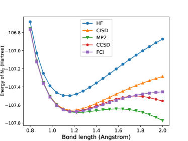
Figure 3: Potential energy curves for the ground state of N2 calculated by various classical computational methods. The ground state energies are calculated by the Hartree-Fock (HF) method, configuration interaction singles and doubles (CISD), second-order Møller–Plesset perturbation theory (MP2), coupled cluster singles and doubles (CCSD), and full configuration interaction (FCI, or exact ground state energy).

Table 4: Properties of the Hamiltonian and the ground state for N2 shown for various values of the bond length. “Pauli terms” is the number of Pauli strings contained in the Hamiltonian, $R$ is the number of computational basis states retained in the approximate expectation value (Eq. (13)) for the exact ground state, and $E_{R}-E_{\rm exact}$ is the difference between the energy expectation values for the truncated state and the exact ground state.

Bond length [Å]	Pauli terms	$R$	$E_{R}-E_{\rm exact}$ [$10^{-4}$ Hartree]
1.0	$2239$	$138$	$7.0$
1.2	$2239$	$183$	$5.5$
1.6	$2239$	$237$	$3.3$
2.0	$2239$	$209$	$1.7$

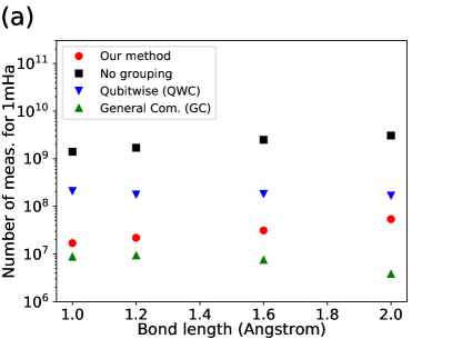
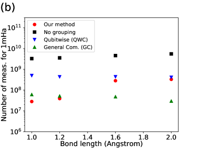
Figure 4: The total number of measurements required to achieve the standard deviation of $10^{-3}$ Hartree in the energy expectation value estimation with the ground state for the nitrogen molecule N2 with various bond lengths, based on a different estimation method and measurement allocation strategy. (a) The results based on the measurement allocations optimized for the exact ground states (obtained by FCI calculations). (b) The results based on the heuristic measurement allocations.

In this section, we perform the same analysis as in Sec. III for the nitrogen molecule N2 with various bond lengths. N2 with a stretched geometry is known as an example for a correlated electron system where the theoretical descriptions based on a single reference state (typically Hartree-Fock state) fail. We investigate whether our method based on the approximation of the wavefunction by a limited number of computational basis states or Slater determinants still works in such a case.

First, we calculate the potential energy curves for the ground state of N2 by various classical computational methods with the STO-3G minimal basis set (Fig. 3). As the bond length becomes larger than the equilibrium distance around 1.2Å, the energies computed by the classical methods based on the single-reference state (HF, CISD, MP2, CCSD) deviate more and more from the exact one. This may indicate that the ground state of stretched N2 is not well-described by a small number of Slater determinants, casting doubt on the assumption of concentration of the state in our approach. But, there may be a possibility that the ground state is still concentrated enough even though the degree of concentration is beyond the capability of those classical methods.

Next, we perform the same analysis as in Sec. III.2 by choosing four different bond lengths: 1.0Å, 1.2Å, 1.6Å, and 2.0Å. In Table 4 (corresponding to Table 1), the number of the Pauli strings in the Hamiltonian and the value of $R$, which is the minimum number of computational basis states satisfying $1-\absolutevalue{\innerproduct{\psi_{R}}{\psi}}^{2}\leq 10^{-4}$, are shown for each bond length. The value of $R$ slightly increases when the bond length becomes larger than 1.2Å, which is close to the equilibrium distance, possibly reflecting the nature of the wavefunction that is not described by the single-reference methods.

Finally, we evaluate the standard deviation in the estimation of energy expectation value for the ground state of N2 in the same way as presented in Sec. III.3 (all the conditions for numerical calculations are taken to be the same). Then, in Fig. 4, the estimation for the total number of measurements to realize the standard deviation of $10^{-3}$ Hartree is shown for each of the bond lengths and for various methods (presented in the similar way as in Fig. 2). Our method gets slightly worse as the bond length increases, but is still more efficient than QWC. The overall tendency of the results between the different methods (no grouping, QWC or general-commuting grouping, and our method) is the same as discussed in Sec. III.3.

The results presented in this section demonstrate a case where our method works efficiently even for a correlated electron system that cannot be well-described by the single-reference methods but still has a concentrated wavefunction. This supports the applicability of our method beyond weakly-correlated molecules.

Appendix H Variance for explicit importance sampling

We point out that the variance of expectation values evaluated by the explicit importance sampling of Eq. (6),

$$\expectationvalue{O}{\psi}={\sum_{m,n}}^{\prime}\absolutevalue{\bra{m}\ket{\psi}}^{2}\absolutevalue{\bra{n}\ket{\psi}}^{2}\frac{\matrixelement{m}{O}{n}}{\bra{m}\ket{\psi}\bra{\psi}\ket{n}},$$ (75)

may be exponentially large in the number of qubits $N$. In the discussion here, we assume the quantum state $\ket{\psi}$ is real for simplicity. Here we mean by the explicit importance sampling that one samples a quantity $f(m,n)=\frac{\matrixelement{m}{O}{n}}{\bra{m}\ket{\psi}\bra{\psi}\ket{n}}$ with a probability of $p(m,n)=\absolutevalue{\bra{m}\ket{\psi}}^{2}\absolutevalue{\bra{n}\ket{\psi}}^{2}$ and takes an average of the results from repeated sampling. If we could evaluate $f(m,n)$ exactly without any sampling error, the variance of the sampling would be

$${\sum_{m,n}}^{\prime}(f(m,n))^{2}p(m,n)-\quantity({\sum_{m,n}}^{\prime}f(m,n)p(m,n))^{2}$$

$$= {\sum_{m,n}}^{\prime}\frac{\matrixelement{m}{O}{n}^{2}}{\bra{m}\ket{\psi}^{2}\bra{\psi}\ket{n}^{2}}\absolutevalue{\bra{m}\ket{\psi}}^{2}\absolutevalue{\bra{n}\ket{\psi}}^{2}-\quantity(\expectationvalue{O}{\psi})^{2}$$

$$= {\sum_{m,n}}^{\prime}\matrixelement{m}{O}{n}^{2}-\quantity(\expectationvalue{O}{\psi})^{2},$$

where we use the assumption that $\innerproduct{n}{\psi}$ and $\innerproduct{m}{\psi}$ are real. When we write a subspace in which the state $\ket{\psi}$ lives as $\mathcal{M}$, i.e., $\mathcal{M}=\mathrm{span}\quantity(\{\ket{n}|\innerproduct{n}{\psi}\neq 0\})$, the first term reads

$${\sum_{m,n}}^{\prime}\matrixelement{m}{O}{n}^{2} ={\sum_{m,n}}^{\prime}\matrixelement{m}{O}{n}\!\matrixelement{n}{O}{m}$$

$$={\sum_{m}}^{\prime}\bra{m}OP_{\mathcal{M}}O\ket{m}$$

$$=\Tr_{\mathcal{M}}[(O|_{\mathcal{M}})^{2}],$$

where $P_{\mathcal{M}}$ is a projection operator onto $\mathcal{M}$ and $O|_{\mathcal{M}}=P_{\mathcal{M}}OP_{\mathcal{M}}$ is the operator $\mathcal{O}$ projected on $\mathcal{M}$. Since the dimension of $\mathcal{M}$ grows exponentially with $N$ in general, $\Tr_{\mathcal{M}}[(O|_{\mathcal{M}})^{2}]$ is $\mathcal{O}(2^{N})$. By considering the fact that $\expectationvalue{O}{\psi}$ is typically $\mathcal{O}(N)$ especially in applications to condensed matter physics and quantum chemistry, the variance of the explicit importance sampling can be exponentially large in some cases, regardless if the state is concentrated. We remark that we here assume $f(m,n)$ can be exactly evaluated but this oversimplifies the case; in actual applications, values of $f(m,n)$ should be also estimated by sampling and hence fluctuate for finite numbers of sampling. We also stress that this analysis would not deteriorate the validity of our results in large quantum systems because our algorithm described in Sec. II.2 is formally different from the explicit importance sampling.

References

- Preskill [2018] J. Preskill, Quantum computing in the NISQ era and beyond, Quantum 2, 79 (2018).
- Cerezo et al. [2021] M. Cerezo, A. Arrasmith, R. Babbush, S. C. Benjamin, S. Endo, K. Fujii, J. R. McClean, K. Mitarai, X. Yuan, L. Cincio, and P. J. Coles, Variational quantum algorithms, Nature Reviews Physics 3, 625 (2021).
- Endo et al. [2021] S. Endo, Z. Cai, S. C. Benjamin, and X. Yuan, Hybrid quantum-classical algorithms and quantum error mitigation, Journal of the Physical Society of Japan 90, 032001 (2021).
- Tilly et al. [2021] J. Tilly, H. Chen, S. Cao, D. Picozzi, K. Setia, Y. Li, E. Grant, L. Wossnig, I. Rungger, G. H. Booth, and J. Tennyson, The variational quantum eigensolver: a review of methods and best practices (2021), arXiv:2111.05176 [quant-ph] .
- Peruzzo et al. [2014] A. Peruzzo, J. McClean, P. Shadbolt, M.-H. Yung, X.-Q. Zhou, P. J. Love, A. Aspuru-Guzik, and J. L. O’Brien, A variational eigenvalue solver on a photonic quantum processor, Nature communications 5, 1 (2014).
- McArdle et al. [2020] S. McArdle, S. Endo, A. Aspuru-Guzik, S. C. Benjamin, and X. Yuan, Quantum computational chemistry, Rev. Mod. Phys. 92, 015003 (2020).
- Cao et al. [2019] Y. Cao, J. Romero, J. P. Olson, M. Degroote, P. D. Johnson, M. Kieferová, I. D. Kivlichan, T. Menke, B. Peropadre, N. P. Sawaya, et al., Quantum chemistry in the age of quantum computing, Chemical reviews 119, 10856 (2019).
- Gonthier et al. [2022] J. F. Gonthier, M. D. Radin, C. Buda, E. J. Doskocil, C. M. Abuan, and J. Romero, Measurements as a roadblock to near-term practical quantum advantage in chemistry: resource analysis quantum advantage through resource estimation: the measurement roadblock in the variational quantum eigensolver, Phys. Rev. Research 4, 033154 (2022).
- McClean et al. [2016] J. R. McClean, J. Romero, R. Babbush, and A. Aspuru-Guzik, The theory of variational hybrid quantum-classical algorithms, New Journal of Physics 18, 023023 (2016).
- Kandala et al. [2017] A. Kandala, A. Mezzacapo, K. Temme, M. Takita, M. Brink, J. M. Chow, and J. M. Gambetta, Hardware-efficient variational quantum eigensolver for small molecules and quantum magnets, Nature 549, 242 (2017).
- Jena et al. [2019] A. Jena, S. Genin, and M. Mosca, Pauli partitioning with respect to gate sets, arXiv preprint arXiv:1907.07859 (2019).
- Izmaylov et al. [2019] A. F. Izmaylov, T.-C. Yen, and I. G. Ryabinkin, Revising the measurement process in the variational quantum eigensolver: is it possible to reduce the number of separately measured operators?, Chem. Sci. 10, 3746 (2019).
- Izmaylov et al. [2020] A. F. Izmaylov, T.-C. Yen, R. A. Lang, and V. Verteletskyi, Unitary partitioning approach to the measurement problem in the variational quantum eigensolver method, Journal of Chemical Theory and Computation 16, 190 (2020).
- Verteletskyi et al. [2020] V. Verteletskyi, T.-C. Yen, and A. F. Izmaylov, Measurement optimization in the variational quantum eigensolver using a minimum clique cover, The Journal of Chemical Physics 152, 124114 (2020).
- Yen et al. [2020] T.-C. Yen, V. Verteletskyi, and A. F. Izmaylov, Measuring all compatible operators in one series of single-qubit measurements using unitary transformations, Journal of Chemical Theory and Computation 16, 2400 (2020).
- Gokhale et al. [2020] P. Gokhale, O. Angiuli, Y. Ding, K. Gui, T. Tomesh, M. Suchara, M. Martonosi, and F. T. Chong, measurement cost for variational quantum eigensolver on molecular hamiltonians, IEEE Transactions on Quantum Engineering 1, 1 (2020).
- Zhao et al. [2020] A. Zhao, A. Tranter, W. M. Kirby, S. F. Ung, A. Miyake, and P. J. Love, Measurement reduction in variational quantum algorithms, Phys. Rev. A 101, 062322 (2020).
- Crawford et al. [2021] O. Crawford, B. van Straaten, D. Wang, T. Parks, E. Campbell, and S. Brierley, Efficient quantum measurement of Pauli operators in the presence of finite sampling error, Quantum 5, 385 (2021).
- Bonet-Monroig et al. [2020] X. Bonet-Monroig, R. Babbush, and T. E. O’Brien, Nearly optimal measurement scheduling for partial tomography of quantum states, Phys. Rev. X 10, 031064 (2020).
- Hamamura and Imamichi [2020] I. Hamamura and T. Imamichi, Efficient evaluation of quantum observables using entangled measurements, npj Quantum Information 6, 56 (2020).
- Huggins et al. [2021] W. J. Huggins, J. R. McClean, N. C. Rubin, Z. Jiang, N. Wiebe, K. B. Whaley, and R. Babbush, Efficient and noise resilient measurements for quantum chemistry on near-term quantum computers, npj Quantum Information 7, 23 (2021).
- Yen and Izmaylov [2021] T.-C. Yen and A. F. Izmaylov, Cartan subalgebra approach to efficient measurements of quantum observables, PRX Quantum 2, 040320 (2021).
- Shlosberg et al. [2021] A. Shlosberg, A. J. Jena, P. Mukhopadhyay, J. F. Haase, F. Leditzky, and L. Dellantonio, Adaptive estimation of quantum observables, arXiv preprint arXiv:2110.15339 (2021).
- Yen et al. [2022] T.-C. Yen, A. Ganeshram, and A. F. Izmaylov, Deterministic improvements of quantum measurements with grouping of compatible operators, non-local transformations, and covariance estimates, arXiv preprint arXiv:2201.01471 (2022).
- Wecker et al. [2015] D. Wecker, M. B. Hastings, and M. Troyer, Progress towards practical quantum variational algorithms, Phys. Rev. A 92, 042303 (2015).
- Rubin et al. [2018] N. C. Rubin, R. Babbush, and J. McClean, Application of fermionic marginal constraints to hybrid quantum algorithms, New Journal of Physics 20, 053020 (2018).
- Arrasmith et al. [2020] A. Arrasmith, L. Cincio, R. D. Somma, and P. J. Coles, Operator sampling for shot-frugal optimization in variational algorithms, arXiv preprint arXiv:2004.06252 (2020).
- Huang et al. [2020] H.-Y. Huang, R. Kueng, and J. Preskill, Predicting many properties of a quantum system from very few measurements, Nature Physics 16, 1050 (2020).
- Zhao et al. [2021] A. Zhao, N. C. Rubin, and A. Miyake, Fermionic partial tomography via classical shadows, Phys. Rev. Lett. 127, 110504 (2021).
- Hadfield et al. [2020] C. Hadfield, S. Bravyi, R. Raymond, and A. Mezzacapo, Measurements of quantum hamiltonians with locally-biased classical shadows, arXiv preprint arXiv:2006.15788 (2020).
- Wu et al. [2021] B. Wu, J. Sun, Q. Huang, and X. Yuan, Overlapped grouping measurement: A unified framework for measuring quantum states, arXiv preprint arXiv:2105.13091 (2021).
- Radin and Johnson [2021] M. D. Radin and P. Johnson, Classically-boosted variational quantum eigensolver, arXiv preprint arXiv:2106.04755 (2021).
- Nielsen and Chuang [2010] M. A. Nielsen and I. L. Chuang, Quantum computation and quantum information, 10th ed. (Cambridge University Press, 2010).
- McMillan [1965] W. L. McMillan, Ground state of liquid , Phys. Rev. 138, A442 (1965).
- Ceperley et al. [1977] D. Ceperley, G. V. Chester, and M. H. Kalos, Monte carlo simulation of a many-fermion study, Phys. Rev. B 16, 3081 (1977).
- Eddins et al. [2022] A. Eddins, M. Motta, T. P. Gujarati, S. Bravyi, A. Mezzacapo, C. Hadfield, and S. Sheldon, Doubling the size of quantum simulators by entanglement forging, PRX Quantum 3, 010309 (2022).
- McClean et al. [2020] J. R. McClean, N. C. Rubin, K. J. Sung, I. D. Kivlichan, X. Bonet-Monroig, Y. Cao, C. Dai, E. S. Fried, C. Gidney, B. Gimby, P. Gokhale, T. Häner, T. Hardikar, V. Havlíček, O. Higgott, C. Huang, J. Izaac, Z. Jiang, X. Liu, S. McArdle, M. Neeley, T. O’Brien, B. O’Gorman, I. Ozfidan, M. D. Radin, J. Romero, N. P. D. Sawaya, B. Senjean, K. Setia, S. Sim, D. S. Steiger, M. Steudtner, Q. Sun, W. Sun, D. Wang, F. Zhang, and R. Babbush, OpenFermion: the electronic structure package for quantum computers, Quantum Science and Technology 5, 034014 (2020).
- Sun et al. [2018] Q. Sun, T. C. Berkelbach, N. S. Blunt, G. H. Booth, S. Guo, Z. Li, J. Liu, J. D. McClain, E. R. Sayfutyarova, S. Sharma, S. Wouters, and G. K.-L. Chan, PySCF: the Python-based simulations of chemistry framework, WIREs Comput. Mol. Sci. 8, e1340 (2018).
- Sun et al. [2020] Q. Sun, X. Zhang, S. Banerjee, P. Bao, M. Barbry, N. S. Blunt, N. A. Bogdanov, G. H. Booth, J. Chen, Z.-H. Cui, J. J. Eriksen, Y. Gao, S. Guo, J. Hermann, M. R. Hermes, K. Koh, P. Koval, S. Lehtola, Z. Li, J. Liu, N. Mardirossian, J. D. McClain, M. Motta, B. Mussard, H. Q. Pham, A. Pulkin, W. Purwanto, P. J. Robinson, E. Ronca, E. R. Sayfutyarova, M. Scheurer, H. F. Schurkus, J. E. T. Smith, C. Sun, S.-N. Sun, S. Upadhyay, L. K. Wagner, X. Wang, A. White, J. D. Whitfield, M. J. Williamson, S. Wouters, J. Yang, J. M. Yu, T. Zhu, T. C. Berkelbach, S. Sharma, A. Y. Sokolov, and G. K.-L. Chan, Recent developments in the pyscf program package, The Journal of Chemical Physics 153, 024109 (2020), https://doi.org/10.1063/5.0006074 .
- Editor: Russell D. Johnson III [2020] Editor: Russell D. Johnson III, NIST Computational Chemistry Comparison and Benchmark Database, NIST Standard Reference Database Number 101, http://cccbdb.nist.gov/ (2020).
- Suzuki et al. [2021] Y. Suzuki, Y. Kawase, Y. Masumura, Y. Hiraga, M. Nakadai, J. Chen, K. M. Nakanishi, K. Mitarai, R. Imai, S. Tamiya, et al., Qulacs: a fast and versatile quantum circuit simulator for research purpose, Quantum 5, 559 (2021).
- Aaronson and Gottesman [2004] S. Aaronson and D. Gottesman, Improved simulation of stabilizer circuits, Physical Review A 70, 052328 (2004).
- Bonet-Monroig et al. [2018] X. Bonet-Monroig, R. Sagastizabal, M. Singh, and T. E. O’Brien, Low-cost error mitigation by symmetry verification, Phys. Rev. A 98, 062339 (2018).
- McArdle et al. [2019] S. McArdle, X. Yuan, and S. Benjamin, Error-mitigated digital quantum simulation, Phys. Rev. Lett. 122, 180501 (2019).
- Temme et al. [2017] K. Temme, S. Bravyi, and J. M. Gambetta, Error mitigation for short-depth quantum circuits, Phys. Rev. Lett. 119, 180509 (2017).
- Endo et al. [2018] S. Endo, S. C. Benjamin, and Y. Li, Practical quantum error mitigation for near-future applications, Phys. Rev. X 8, 031027 (2018).
- Helgaker et al. [2014] T. Helgaker, P. Jorgensen, and J. Olsen, Molecular electronic-structure theory (John Wiley & Sons, 2014).
- Jensen [2017] F. Jensen, Introduction to computational chemistry (John wiley & sons, 2017).
- Sabzevari and Sharma [2018] I. Sabzevari and S. Sharma, Improved speed and scaling in orbital space variational monte carlo, Journal of Chemical Theory and Computation 14, 6276 (2018).
- Mahajan and Sharma [2020] A. Mahajan and S. Sharma, Efficient local energy evaluation for multi-slater wave functions in orbital space quantum monte carlo, The Journal of Chemical Physics 153, 194108 (2020).
- Anand et al. [2022] A. Anand, P. Schleich, S. Alperin-Lea, P. W. K. Jensen, S. Sim, M. Díaz-Tinoco, J. S. Kottmann, M. Degroote, A. F. Izmaylov, and A. Aspuru-Guzik, A quantum computing view on unitary coupled cluster theory, Chem. Soc. Rev. 51, 1659 (2022).
- Huggins et al. [2022] W. J. Huggins, B. A. O’Gorman, N. C. Rubin, D. R. Reichman, R. Babbush, and J. Lee, Unbiasing fermionic quantum monte carlo with a quantum computer, Nature 603, 416 (2022).
- Tubman et al. [2016] N. M. Tubman, J. Lee, T. Y. Takeshita, M. Head-Gordon, and K. B. Whaley, A deterministic alternative to the full configuration interaction quantum monte carlo method, The Journal of Chemical Physics 145, 044112 (2016).
- Evangelista [2014] F. A. Evangelista, Adaptive multiconfigurational wave functions, The Journal of Chemical Physics 140, 124114 (2014).
- Holmes et al. [2016] A. A. Holmes, N. M. Tubman, and C. J. Umrigar, Heat-bath configuration interaction: An efficient selected configuration interaction algorithm inspired by heat-bath sampling, Journal of Chemical Theory and Computation 12, 3674 (2016).
- Schriber and Evangelista [2016] J. B. Schriber and F. A. Evangelista, Communication: An adaptive configuration interaction approach for strongly correlated electrons with tunable accuracy, The Journal of Chemical Physics, The Journal of Chemical Physics 144, 161106 (2016).
- Tubman et al. [2020] N. M. Tubman, C. D. Freeman, D. S. Levine, D. Hait, M. Head-Gordon, and K. B. Whaley, Modern approaches to exact diagonalization and selected configuration interaction with the adaptive sampling ci method, Journal of Chemical Theory and Computation 16, 2139 (2020).
- Bravyi and Kitaev [2002] S. B. Bravyi and A. Y. Kitaev, Fermionic quantum computation, Annals of Physics 298, 210 (2002).