Stochastic Planner-Actor-Critic for Unsupervised Deformable Image Registration

Abstract

Large deformations of organs, caused by diverse shapes and nonlinear shape changes, pose a significant challenge for medical image registration. Traditional registration methods need to iteratively optimize an objective function via a specific deformation model along with meticulous parameter tuning, but which have limited capabilities in registering images with large deformations. While deep learning-based methods can learn the complex mapping from input images to their respective deformation field, it is regression-based and is prone to be stuck at local minima, particularly when large deformations are involved. To this end, we present Stochastic Planner-Actor-Critic (SPAC), a novel reinforcement learning-based framework that performs step-wise registration. The key notion is warping a moving image successively by each time step to finally align to a fixed image. Considering that it is challenging to handle high dimensional continuous action and state spaces in the conventional reinforcement learning (RL) framework, we introduce a new concept ‘Plan’ to the standard Actor-Critic model, which is of low dimension and can facilitate the actor to generate a tractable high dimensional action. The entire framework is based on unsupervised training and operates in an end-to-end manner. We evaluate our method on several 2D and 3D medical image datasets, some of which contain large deformations. Our empirical results highlight that our work achieves consistent, significant gains and outperforms state-of-the-art methods. Code is available at https://github.com/Algolzw/SPAC-Deformable-Registration

Introduction

Deformable image registration (DIR) is an important task in medical imaging and has been actively studied for decades. DIR consists of establishing a spatial anatomical non-linear dense correspondence between a pair of fixed and moving images. The central task of DIR is the estimation of the ill-posed free-form transformation field that consists of a combination of global and local displacements (Eppenhof et al. 2019). Moreover, an accurate DIR on large deformation is needed due to soft organs (e.g., the brain, liver, and stomach) may undergo large deformations caused by patient re-positioning, surgical manipulation, or other physiological differences (Holden 2007). Large deformation diffeomorphic metric mapping (LDDMM) (Beg et al. 2005), derived from the group structure of the manifold of diffeomorphisms, is one of the most popular methods to tackle large deformations in DIR. However, achieving an optimal solution of the diffeomorphic image registration is computationally intensive and time-consuming, attempts at speeding up diffeomorphic image registration have thus been proposed to improve numerical approximation schemes (Wang and Zhang 2020).

Most existing DL-based solutions (Balakrishnan et al. 2019; Dalca et al. 2019; Mok and Chung 2020) are enforced to make a straightforward prediction, which is incapable to handle complicated deformations (Zhao et al. 2019). The step-wise image registration methods, such as R2N2 (Sandkühler et al. 2019) and RCN (Zhao et al. 2019), have shown the potential in DIR, in which the final deformation field (probably with large displacements) can be considered as a composition of the progressively predicted deformation field. But both of them are complex and computationally costly, and cannot deal with long step-wise registration. Inspired by the way that a human expert aligns two images by applying a sequence of local or global deformations, some RL-based image registration methods have been introduced in the past (Liao et al. 2017; Ma et al. 2017; Miao and Liao 2019; Sun et al. 2018; Hu et al. 2021; Luo et al. 2020). However, most of them merely focus on global rigid transformation since it only includes rotation and translation and can be easily represented by a low-dimensional discrete parametric model. Compared to rigid registration, DIR has huge, continuous state and action spaces, especially in 3D, which makes RL training extremely difficult. Krebs et al. (Krebs et al. 2017) proposed an RL-based approach for DIR, but their method uses supervised learning with ground truth deformation field, which is infeasible for most DIR tasks. And they incorporate the traditional statistical deformation model to reduce and discretize the action space, which leads to inferior performance in complex deformation registration.

In this paper, we propose a new RL architecture for unsupervised DIR problems, known as the Stochastic Planner-Actor-Critic (SPAC), to handle high dimensional continuous state and action spaces. As shown in Figure 1, the SPAC framework is formed with three core deep neural networks: the planner, the actor, and the critic. We introduce new a concept ‘plan’ which breaks the decision-making process into two steps, state $\rightarrow$ plan and plan $\rightarrow$ action. We call this process as meta policy, where the plan is a subspace of appropriate actions based on the current state, but it is not applied to the state directly, it is used to guide the actor to generate a tractable high-dimensional action that applies to the environment. The plan could be considered as an intermediate transition between state and action. As the input of the actor, the plan has a much lower dimension comparing with the state, which is easier for the actor to learn to predict actions. Meanwhile, the plan can be evaluated by the critic efficiently, since the Q function is easier to learn in the low-dimensional latent space. Furthermore, we employ an unsupervised registration learning strategy to learn the similarity of appearance between fixed and moving image pairs. The main contributions of our work can be summarized as follows:

• We describe a new RL framework, stochastic planner-actor-critic (SPAC), to handle large deformations by decomposing the monolithic learning process in DIR into small steps with high-dimensional continuous actions.

• To tackle the high-dimensional continuous action learning problem, we propose a stochastic meta policy that breaks the decision-making processing into two steps: state $\rightarrow$ low-dimensional plan and plan $\rightarrow$ deformation field action. The plan guides the actor to predict a tractable action, and the critic evaluates the plan, which makes the whole learning process feasible and computationally efficient.

• We design an registration environment which incorporates a K-means clustering module (Dice 1945) to obtain coarse segmentation maps to compute the Dice reward in an unsupervised manner, which obviates the need to collect real data with abundant and reliable ground-truth annotations. Besides, our method can be applied to entire 3D volumes.

• Experimental results on a variety of 2D/3D datasets show that the SPAC achieves state-of-the-art performance and consistently improves the results along with iterations.

Background

Deformable Image Registration

Deformable image registration (DIR) aims to learn a transformation between a fixed image and a moving image (Yang, Kwitt, and Niethammer 2016; Balakrishnan et al. 2018; de Vos et al. 2019). The DIR can be defined as an optimization problem. Given a pair of images ($I_{F},I_{M}$), both of which on the image domain ${\cal X}\rightarrow\mathbb{R}^{d}$, where $d$ is the dimension. $I_{F}$ is the fixed image and $I_{M}$ is the moving image. Denote $\Omega_{w}$ as a registration model parameterized by $w$. The output of it is a deformation filed, which can be warped on the moving image to align to the fixed image, denoted as $I_{M}\circ\Omega_{w}(I_{F},I_{M})$. We formulated the pairwise registration as a minimization problem based on energy function:

$$\min_{w}E(w):=G(I_{F},I_{M}\circ\Omega_{w}(I_{F},I_{M}))+\lambda R(\Omega_{w}(I_{F},I_{M}))$$ (1)

where $G$ represents a metric quantifying the similarity between the fixed image and the warped image, $R$ represents a regularization constraining the deformation field, $\lambda$ is a hyperparameter to balance these two terms. In the DL-based DIR task, the DL model tries to learn $\Omega_{w}(I_{F},I_{M})$ from a training dataset, which contains a large number of image pairs ($I_{F},I_{M}$). The potential choice of $G$ could be any similarity metric, such as the sum of squared differences (SSD), the normalized mutual information (NMI), or the negative normalized cross-correlation (NCC) (Haskins, Kruger, and Yan 2020; Balakrishnan et al. 2018).

Reinforcement Learning

RL is described by an infinite-horizon Markov decision process (MDP), defined by the tuple $({\cal S},{\cal A},{\cal U},{r},{\gamma})$. ${\cal S}$ is a set of states, ${\cal A}$ is action, and ${\cal U}:{\cal S}\times{\cal S}\times{\cal A}\rightarrow[0,\infty)$ represents the state transition probability density given state $s\in{\cal S}$ and action ${\bf a}\in{\cal A}$. ${r}:{\cal S}\times{\cal A}\rightarrow\mathbb{R}$ is the reward emitted from each transition, and $\gamma\in[0,1]$ is the reward discount factor. Standard RL learns to maximize the expected sum of rewards from the episodic environments under the trajectory distribution ${\rho}_{\pi}$. It can be modified to incorporate an entropy term with the policy. Therefore, the resulting objective is defined as $\sum\nolimits_{t=1}^{T}\mathbb{E}_{({\bf s}_{t},{\bf a}_{t})\sim{\rho}_{\pi}}\left[r_{t}({\bf s}_{t},{\bf a}_{t})+\alpha{\cal H}(\pi_{\phi}(\cdot|{\bf s}_{t}))\right]$, where $\alpha$ is a temperature parameter controlling the balance of the entropy ${\cal H}$ and the reward $r_{t}$.

Soft Actor-critic (SAC) (Haarnoja et al. 2018) is a promising framework for learning continuous actions, which is an off-policy actor-critic method that uses the above entropy-based framework to derive the soft policy iteration. Stochastic latent actor-critic (SLAC) improves the SAC by learning the representation spaces with a latent variable model which is more stable and efficient for complex continuous control tasks. It can improve both the exploration and robustness of the learned model. However, SLAC is far from enough for handling DIR, which has huge continuous action spaces such as voxel-wise estimation of a deformation field.

Stochastic Planner-Actor-Critic

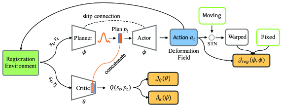
Figure 1: The network architecture of the proposed SPAC  for DIR problem. At time step $t$, the registration environment receives action ${\bf a}_{t}$, and outputs state and reward ($s_{t},r_{t}$). The plan ${\bf p}_{t}$ is sampled from the planner and evaluated by the critic. The action ${\bf a}_{t}$ is actually an immediate deformation field based on state $s_{t}$. The spatial transformer network (STN) is used as the warping function.

Concretely, in our framework, the SPAC is formed with three core deep neural networks: the planner, the actor, and the critic with parameters $\psi$, $\phi$, and $\theta$, respectively (see Figure 1). The planner aims to generate a high-level plan in the low-dimensional latent space to guide the actor. In some sense, the plan can be considered as action clusters or action templates, which are high-level crude actions. Different from classic actor-critic models, the input of the actor is a stochastic plan instead of the state. That is, the generated plan is forwarded to the actor to further create the high dimensional action for DIR, and meanwhile, this plan is evaluated by the critic. We also add skip-connections from each down-sampling layer of the planner to the corresponding up-sampling layer of the actor. The information passed by skip-connections contains the details of the state ${\bf s}_{t}$ that are needed to reconstruct a natural-looking image. Using the proposed stochastic planner-actor-critic structure and supervision of similarity of appearance between fixed and moving image, SPAC could extend readily to complex DIR tasks.

Problem Formulation

In forming SPAC, we apply the same notations as we defined for the conventional reinforcement learning in background section and introduce an additional component ${\cal P}$ for the continuous plan space to the infinite-horizon Markov decision process (MDP). Therefore, the MDP for SPAC can be defined by the tuple $({\cal S},{\cal P},{\cal A},{\cal U},{r},{\gamma})$. ${\cal S}$ is a set of states, ${\cal P}$ is continuous plan, ${\cal A}$ is continuous action, and ${\cal U}:{\cal S}\times{\cal P}\times{\cal S}\times{\cal A}\rightarrow[0,\infty)$ represents the state transition probability density of the next state $s_{t+1}$ given state ${\bf s}_{t}\in{\cal S}$, plan $p_{t}\in{\cal P}$ and action ${\bf a}_{t}\in{\cal A}$.

Step-wise Deformable Registration.

Leveraging the sequential characteristic of reinforcement learning, we decompose the registration into $T$ steps instead of predicting the deformation field in one-shot. At time step $t$, action ${\bf a}_{t}$ is the current deformation field generated by the Planner $\kappa_{\psi}$ and Actor $\pi_{\phi}$ based on fixed image $I_{F}$ and intermediate moving image $I_{M_{t}}$. Let $\Omega^{t}_{\psi,\phi}$ represents the accumulated deformation field composed by ${\bf a}_{t}$ and the previous deformation field $\Omega^{t-1}_{\psi,\phi}$. We can compute $\Omega^{t}_{\psi,\phi}$ with a recursive composition function:

$$\Omega^{t}_{\psi,\phi}=\begin{cases}0&\mbox{if $t=0$,}\\ {\cal C}({\bf a_{t}},\Omega^{t-1}_{\psi,\phi})&\mbox{otherwise,}\end{cases}$$ (2)

where

$$\ {\cal C}({\bf a_{t}},\Omega^{t-1}_{\psi,\phi})=\Omega^{t-1}_{\psi,\phi}+({\bf a}_{t}\circ\Omega^{t-1}_{\psi,\phi}).$$ (3)

To eliminate the warping bias in the multi-step recursive registration process (Zhao et al. 2019), we warp the initial moving image $I_{M}$ using accumulated the deformation field $\Omega^{t}_{\psi,\phi}$. Then the warped image $I_{M_{t+1}}$ is used as the next moving image in time step $t+1$. Therefore, the registration result can be progressively improved by predicting deformation from coarse to the local refined. Using the notion of step-wise, the DIR optimization problem (Eq.(1)) in our SPAC framework can be rewritten as

$$\min_{\psi,\phi}E({\psi,\phi}):=\frac{1}{T}\sum_{t=1}^{T}G(I_{F},I_{M_{t}}\circ\Omega^{t}_{\psi,\phi})+\lambda R(\Omega^{t}_{\psi,\phi}),$$ (4)

where we use a tuple ($\psi,\phi$) instead of the parameter $w$ in Eq.(1) since the deformation field will be learned from the SPAC framework. In the following, we provide the details of the environment and policy in our method.

DIR Environment

The overview of the step-wise deformable registration environment is shown in Figure 2. In the beginning, the environment only contains an image pair ($I_{F}$, $I_{M}$), then we performs K-means (MacQueen et al. 1967) with three clustering labels to obtain the corresponding segmentation maps ($U_{F}$, $U_{M}$) in an unsupervised manner. The generated segmentation map assigns each voxel to a virtual anatomical structure, which facilitates computing rewards. At time step $t$, the state ${\bf s}_{t}$ is the pair of fixed image $I_{F}$ and moving image $I_{M_{t}}$, ${\bf s}_{t}=(I_{F},I_{M_{t}})$. The next state $s_{t+1}$ is obtained by warping $I_{M}$ with composed deformable field $\Omega^{t}_{\psi,\phi}$: $s_{t+1}=(I_{F},I_{M}\circ\Omega^{t}_{\psi,\phi})$. We incorporate the widely used spatial transformer network (STN) (Jaderberg et al. 2015) as the warping operator. The reward ${r_{t}}$ is defined based on the Dice (Dice 1945) score:

$$r_{t}={\rm Dice}(U_{F},U_{M}\circ\Omega^{t}_{\psi,\phi})-{\rm Dice}(U_{F},U_{M}\circ\Omega^{t-1}_{\psi,\phi}),$$ (5)

where ${\rm Dice}(U_{1},U_{2})=2\cdot\frac{|U_{1}\cap U_{2}|}{|U_{1}|+|U_{2}|}$. This reward function explicitly assesses the improvement of the predicted deformation field $\Omega^{t}_{\psi,\phi}$.

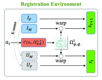
Figure 2: The architecture of the step-wise deformable registration environment. When the environment receives an action ${\bf a}_{t}$, it outputs the next state $s_{t+1}$ and reward $r_{t}$. Specifically, the environment is composed by a pair of image ($I_{F}$, $I_{M}$), and generates the corresponding segmentation maps ($U_{F}$, $U_{M}$) with K-means clustering. ${\cal C}(a_{t},\Omega^{t-1}_{\psi,\phi})$ is the compose function which composes action $a_{t}$ to the accumulated deformation field $\Omega^{t}_{\psi,\phi}$. The next state $s_{t+1}$ is obtained by concatenating $I_{F}$ and the warped moving image $I_{M}\circ\Omega^{t}_{\psi,\phi}$. The reward $r_{t}$ is obtained by Eq. (5) which represents the improvement of Dice score.

Stochastic Meta Policy

In our formulation, we have a meta policy ($\kappa,\pi$), where the stochastic plan is modeled as a subspace of the deformation field that gives low-dimensional vector ${\bf p}_{t}$ given state ${\bf s}_{t}$. While the actor’s action is actually a deterministic deformation field ${\bf a}_{t}$ determined by the plan ${\bf p}_{t}$. Consider a parameterized planner $\kappa_{\psi}$ and actor $\pi_{\phi}$, the stochastic plan is sampled as a representation: ${\bf p}_{t}\sim\kappa_{\psi}({\bf p}_{t}|{\bf s}_{t})$, and the action is generated by decoding the plan vector ${\bf p}_{t}$ to a high-dimensional deformation field: ${\bf a}_{t}=\pi_{\phi}({\bf a}_{t}|{\bf p}_{t})$ In practice, we reparameterize the the planner and the stochastic plan jointly using a neural network approximation ${\bf p}_{t}=f_{\psi}({\bf\epsilon}_{t},{\bf s}_{t})$, known as reparameterization trick (Kingma and Welling 2013), where ${\bf\epsilon}_{t}$ is an input noise vector sampled from a fixed Gaussian distribution. Moreover, we maximize the entropy of plan to improve exploration and robustness. The augmented objective function is formulated as:

$$\max_{\psi,\phi}\sum\limits_{t=1}^{T}\mathbb{E}_{({\bf s}_{t},{\bf p}_{t},{\bf a}_{t})\sim{\rho}_{(\kappa,\pi)}}\left[r_{t}({\bf s}_{t},{\bf p}_{t},{\bf a}_{t})+\alpha{\cal H}(\kappa_{\psi}(\cdot|{\bf s}_{t}))\right].$$

where $\alpha$ is the temperature and ${\rho}_{(\kappa,\pi)}$ is a trajectory distribution under $\kappa_{\psi}({\bf p}_{t}|{\bf s}_{t})$ and $\pi_{\phi}({\bf a}_{t}|{\bf p}_{t})$.

Learning Planner and Critic

Different from conventional RL algorithms, the critic $Q_{\theta}$ evaluates plan ${\bf P}_{t}$ instead of action ${\bf a}_{t}$. since learning a low-dimensional plan in the DIR problem is easier and more effective. Specifically, the low-dimensional plan is concatenated to the downsampled vector of the critic and outputs soft Q function $Q_{\theta}({\bf s}_{t},{\bf p}_{t})$ which is an estimation of the current state plan value, as shown in Figure 1.

When the critic is used to evaluate the planner, the rewards and the soft Q values are used to iteratively guide the stochastic policy improvement. In the evaluation step, following SAC (Haarnoja et al. 2018), SPAC learns a policy $\kappa_{\psi}$ (planner) and fits the parametric Q-function $Q_{\theta}({\bf s}_{t},{\bf p}_{t})$ (critic) using transitions sampled from the replay pool $\mathcal{D}$ by minimizing the soft Bellman residual:

$$J_{Q}(\theta)=$$

$$\mathbb{E}_{({\bf s}_{t},{\bf p}_{t})\sim\mathcal{D}}\left[\frac{1}{2}\Big{(}Q_{\theta}({\bf s}_{t},{\bf p}_{t})-\big{(}r_{t}+\gamma\mathbb{E}_{{\bf s}_{t+1}}\left[V_{\bar{\theta}}({\bf s}_{t+1})\right]\big{)}\Big{)}^{2}\right],$$

where $V_{\bar{\theta}}({\bf s}_{t})=\mathbb{E}_{{\bf p}_{t}\sim\kappa_{\psi}}[Q_{\bar{\theta}}({\bf s}_{t},{\bf p}_{t})-\alpha\log\kappa_{\psi}({\bf p}_{t}|{\bf s}_{t})]$. We use a target network $Q_{\bar{\theta}}$ to stabilize training, whose parameters $\bar{\theta}$ are obtained by an exponentially moving average of parameters of the critic network (Lillicrap et al. 2015): $\bar{\theta}\rightarrow\tau\theta+(1-\tau)\bar{\theta}$. The hyper-parameter $\tau\in[0,1]$. To optimize the $J_{Q}(\theta)$, we can do the stochastic gradient descent with respect to the parameters $\theta$ as follows,

$$\theta=\theta -\eta_{Q}\triangledown_{\theta}Q_{\theta}({\bf s}_{t},{\bf p}_{t})\Big{(}Q_{\theta}({\bf s}_{t},{\bf p}_{t})-r_{t}$$ (6)

$$-\gamma\left[Q_{\bar{\theta}}({\bf s}_{t+1},{\bf p}_{t+1})-\alpha\log\kappa_{\psi}({\bf p}_{t+1}|{\bf s}_{t+1})\right]\Big{)}.$$

Since the critic works on the planner, the optimization procedure will also influence the planner decisions. Following (Haarnoja et al. 2018), we can use the following objective to minimize the KL divergence between the policy and a Boltzmann distribution induced by the Q-function,

$$J_{\kappa}(\psi)= \mathbb{E}_{{\bf s}_{t}\sim\mathcal{D}}\big{[}\mathbb{E}_{{\bf p}_{t}\sim\kappa_{\psi}}\left[\alpha\log(\kappa_{\psi}({\bf p}_{t}|{\bf s}_{t}))-Q_{\theta}({\bf s}_{t},{\bf p}_{t})\right]\big{]}$$

$$= \mathbb{E}_{{\bf s}_{t}\sim\mathcal{D},{\bf\epsilon}_{t}\sim\mathcal{N}(\mu,\sigma)}\big{[}\alpha\log(\kappa_{\psi}(f_{\psi}({\bf\epsilon}_{t},{\bf s}_{t})|{\bf s}_{t}))$$

$$\phantom{=\;;;;;;;;;;;;;;;;;;;;;;;;}-Q_{\theta}({\bf s}_{t},f_{\psi}({\bf\epsilon}_{t},{\bf s}_{t}))\big{]}.$$

The last equation holds because ${\bf p}_{t}$ can be evaluated by $f_{\psi}({\bf\epsilon}_{t},{\bf s}_{t})$ as we discussed before. It should be mentioned that the hyperparameter $\alpha$ can be automatically adjusted by using one proposed method from (Haarnoja et al. 2018). Then we can apply the stochastic gradient method to optimize parameters as follows,

$$\psi= \psi-\eta_{\psi}\Big{(}\triangledown_{\psi}\alpha\log(\kappa_{\psi}(p_{t}|s_{t}))+$$ (7)

$$\big{(}\triangledown_{p_{t}}\alpha\log(\kappa_{\psi}(p_{t}|s_{t}))-\triangledown_{p_{t}}Q_{\theta}(s_{t},p_{t})\big{)}\triangledown_{\psi}f_{\psi}(\epsilon_{t},s_{t})\Big{)}.$$

Learning Planner and Actor with Unsupervised Registration

After getting action ${\bf a}_{t}$ and following meta policy ($\kappa_{\psi},\pi_{\phi}$), we can obtain $\Omega^{t}_{\psi,\phi}$ based on Eq.(2). We learn the similarity of appearance between the fixed image and the warped image using local normalized cross-correlation (NCC) (Balakrishnan et al. 2018): $G(I_{F},I_{M_{t}})=NCC(I_{F},I_{M}\circ\Omega^{t}_{\psi,\phi})$. A higher value of the NCC indicates a better alignment.

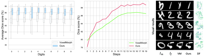
Figure 3: Left: The plot box of Dice scores over 9 fixed digits. Center: Step-wise comparison of our method and VoxelMorph (VM) (Balakrishnan et al. 2018). Right: Visual comparison of our method with VM. The scaled and rotated digits are transformed to other fixed digits. The Deformation Filed (DF) column shows the visualized deformable fields of our method.

In order to generate realistic warped images, we use a total variation regularizer (Rudin, Osher, and Fatemi 1992) to smooth the deformation field on its spatial gradients: $R(\Omega^{t}_{\psi,\phi})=\|\nabla\Omega^{t}_{\psi,\phi}\|^{2}_{2}$ . The final registration loss $J_{reg}$ is defined as

$$J_{reg}(\psi,\phi)= \mathbb{E}_{s_{t}\sim{\cal D}}[-NCC(I_{F},I_{M}\circ\Omega^{t}_{\psi,\phi})+\lambda\|\nabla\Omega^{t}_{\psi,\phi}({\bf s}_{t})\|^{2}_{2}].$$

We can update $\psi$ and $\phi$ from the planner and the actor by performing the following steps:

$$\psi=\psi-\eta\triangledown_{\psi}J_{reg}(\psi,\phi),\ \ \ \phi=\phi-\eta\triangledown_{\phi}J_{reg}(\psi,\phi)$$ (8)

The pseudo-code of optimizing SPAC is described in Algorithm 1. All parameters of SPAC are optimized base on the samples from replay pool $\cal D$.

Input: $I_{F}$, $I_{M}$, $U_{F}$, $U_{M}$, replay pool $\mathcal{D}$

Init: $\psi$, $\phi$, $\theta$, $\bar{\theta}$, $\mathcal{D}$ and environment $\cal E$

for each iteration do

       for each environment step do

             ${\bf p}_{t}\sim\kappa_{\psi}({\bf p}_{t}|{\bf s}_{t})$, ${\bf a}_{t}\sim\pi_{\phi}({\bf a}_{t}|{\bf p}_{t})$

            ${\bf s}_{t+1},{r_{t}}\sim\mathcal{U}({\bf s}_{t+1}|{\bf s}_{t},{\bf p}_{t},{\bf a}_{t})$

            $\mathcal{D}=\mathcal{D}\cup\{({\bf s}_{t},{\bf p}_{t},{\bf a}_{t},r_{t},s_{t+1})\}$

       end for

      

      for each gradient step do

             Sample from $\mathcal{D}$

            Update $\theta$, $\psi$, $\phi$ with Eq.(6), Eq.(7), Eq. (8)

       end for

      

end for

Algorithm 1 Stochastic Planner-Actor-Critic

Experiments

Experimental Settings

Datasets.

We evaluate our method on three types of images: MNIST digits, 2D brain MRI scans, and 3D liver CT scans. MNIST (LeCun et al. 1998) is regarded as a standard sanity check for the proposed registration method. The goal is to transform between two different $28\times 28$ images of handwritten digits. In testing, we fixed ten digits from 0 to 9 as the atlases, and select 1000 randomly scaled and rotated digits as moving images to be aligned with the atlas.

The 2D brain MRI training dataset consists of 2302 pre-processed 2D scans from ADNI (Mueller et al. 2005), ABIDE (Di Martino et al. 2014) and ADHD (Bellec et al. 2017). The evaluation dataset uses 40 pre-processed slices from LONI Probabilistic Brain Atlas (LPBA) (Shattuck et al. 2008), each of which contains a segmentation ground truth of 56 manually delineated anatomical structures. All images are resampled to $128\times 128$ pixels. The first slice of LPBA is served as the atlas, and all the remaining images are used as the moving image. For 3D registration, we use Liver Tumor Segmentation (LiTS) (Bilic et al. 2019) challenge data for training, which contains 131 CT scans with the segmentation ground truth manually annotated by experts. The SLIVER (Heimann et al. 2009) dataset has 20 scans with liver segmentation ground truth. We divide them into 10 pairs as the regular testing data. We also evaluated our method on the challenging Liver Segmentation of Pigs (LSPIG) (Zhao et al. 2019) dataset, which contains 17 paired CT scans from pigs, along with liver segmentation ground truth. All 3D volumes are resampled to $128\times 128\times 128$ pixels and pre-affined as standard pre-processing steps.

Method	2D Registration			3D Registration
	LPBA	Time(s)	#Params	SLIVER	LSPIG	Time(s)	#Params
SyN (Avants et al. 2008)	55.47$\pm$3.96	4.57	-	89.57$\pm$3.34	81.83$\pm$8.30	269	-
Elastix (Klein et al. 2009)	53.64$\pm$3.97	2.20	-	90.23$\pm$2.39	81.19$\pm$7.47	87.0	-
LDDMM (Beg et al. 2005)	52.18$\pm$3.48	3.27	-	83.94$\pm$3.44	82.33$\pm$7.14	41.4	-
VM (Balakrishnan et al. 2019)	55.36$\pm$3.94	0.02	105K	86.37$\pm$4.15	81.13$\pm$7.28	0.13	356K
VM-diff (Dalca et al. 2019)	55.88$\pm$3.78	0.02	118K	87.24$\pm$3.26	81.38$\pm$7.21	0.16	396K
R2N2 (Sandkühler et al. 2019)	51.84$\pm$3.30	0.46	3,591K	-	-	-	-
RCN (Zhao et al. 2019)	-	-	-	89.59$\pm$3.18	82.87$\pm$5.69	2.44	21,291K
SYMNet (Mok and Chung 2020)	-	-	-	86.97$\pm$3.82	82.78$\pm$7.20	0.18	1,124K
SPAC ($t$=20, SSIM reward)	56.43$\pm$3.76	0.16	107K	90.27$\pm$3.85	83.69$\pm$6.74	1.05	458K
SPAC ($t$=1, Dice reward)	55.21$\pm$3.55	0.02	107K	84.81$\pm$4.42	80.61$\pm$7.94	0.07	458K
SPAC ($t$=10, Dice reward)	56.12$\pm$3.68	0.08	107K	90.01$\pm$3.79	84.67$\pm$6.05	0.55	458K
SPAC ($t$=20, Dice reward)	56.57$\pm$3.71	0.16	107K	90.28$\pm$3.66	84.40$\pm$6.24	1.05	458K

Table 1: Dice score (%) results of our SPAC  ($t$ indicates the $t$-th step) with other methods over all datasets. The running times of 3D registration is test on SLIVER dataset. Note that R2N2 works only for 2D registration. The official RCN and SYMNet are implemented only for 3D registration.

Baselines.

This work focus on unsupervised deformable registration. We compare our method with several deep learning based image registration (DLIR) methods: VoxelMorph (VM) (Balakrishnan et al. 2019), VM-diff (Dalca et al. 2019), SYMNet (Mok and Chung 2020), R2N2 (Sandkühler et al. 2019) and RCN (Zhao et al. 2019). VM employs a U-Net structure with NCC loss to learn deformable registration, and VM-diff is a probabilistic diffeomorphic variant of VM. SYMNet is a state-of-the-art single-pass 3D registration method. R2N2 and RCN are sequence-based methods for 2D and 3D registration, respectively. To illustrate the effectiveness of the proposed method, we use the same network structure as VM. We also compare with two top-performing conventional registration algorithms, SyN (Avants et al. 2008) and Elastix (Klein et al. 2009) with B-Spline (Rueckert et al. 1999). In addition, we provide the result of using SSIM as the reward function. We use Dice score as the evaluation metric.

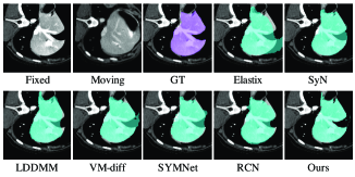
Figure 4: Visual results of our SPAC with other methods on 3D liver dataset. The warped moving image obtained by our SPAC is closer to the ground truth.

Experimental Results

MNIST Digits Transform.

Figure 3 shows the representative results and average Dice scores on MNIST digits transforms. In testing, the moving images are randomly scaled and rotated, which results in a larger and more challenging deformation field. Our method outperforms VM over all kinds of digits with significant improvements quantitatively and qualitatively, which also demonstrates that the proposed method has better generalizability and can work well on image pairs with large deformations.

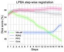
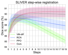
Figure 5: Step-wise registration results overall datasets. The RL-based methods (Our SPAC  and PPO) perform more stable than other DL-based methods, and our SPAC  achieved the best performance.

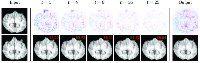
Figure 6: A step-wise registration example of our method on the LPBA dataset. Top row is the visualized displacement field, where deep color represents a large deformation. The Dice score (red) keeps increasing along the steps.

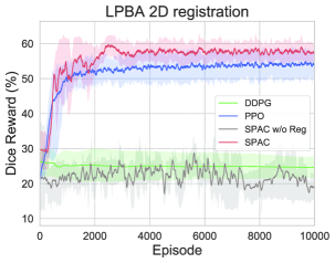
Figure 7: Learning curves of several RL-based methods on LPBA dataset.

Medical Image Registration.

Table 1 summarizes the performance of our method with other state-of-the-art methods. The SPAC outperforms other methods over all 2D and 3D datasets. Moreover, the LSPIG dataset has large deformation fields and is quite different from the training dataset (LiTS) in structure and appearance. The quantitative results on LSPIG illustrate that our framework works well in large deformation dataset and has better generalizability than other conventional DL-based methods. Note that our method performs registration in a step-wise manner, which results in a slower speed than most one-step methods such as VM and SYMNet. But SPAC is still faster than other multi-step methods such as R2N2 and RCN. The SSIM reward based SPAC  achieve good result on SLIVER but performs worse on LSPIG dataset compared with Dice reward based SPAC . We visualized an example of registration results on the LSPIG dataset by overlaying the warped moving segmentation map on the fixed image in Figure 4. The result shows that our model successfully learns registration even with a challenging, large deformation. The SPAC exceeds the performance of another step-wise method RCN, which demonstrates the effectiveness of our framework.

Analysis

Step-wise registration.

The key idea of our method is to decompose the monolithic registration process into small steps by a lighter-weight CNN and progressively improves the transformed results. Figure 6 shows an example of step-wise registration process. The deformation fields visualized on the upper row illustrate that our method predicts transformation from coarse to the local refines step by step. We compared our method with PPO (Schulman et al. 2017) and other DL-based methods using step-wise registration in Figure 5. As the registration step increases, the performance of DL-based methods gets worse, while the RL-based methods are more stable. The Dice score of SPAC is increasing all the time on LPBA and SLIVER datasets.

	LPBA	SLIVER	LSPIG
PPO-modified	55.82$\pm$3.49	89.30$\pm$3.63	83.55$\pm$6.24
SPAC-action	55.58$\pm$3.70	88.75$\pm$3.69	81.80$\pm$7.51
SPAC w/o RL	54.89$\pm$3.80	85.43$\pm$4.14	80.72$\pm$7.34
SPAC w/o Reg	44.67$\pm$3.74	79.34$\pm$4.02	72.45$\pm$6.25
SPAC	56.57$\pm$3.71	90.28$\pm$3.66	84.40$\pm$6.24

Table 2: Dice score (%) over several variants of our methods. ‘SPAC-action’ indicates that the critic evaluates the actor’s action instead of planner in SPAC.

Compare with other RL methods.

To demonstrate our method in the reinforcement learning side. We modify our framework with other popular RL algorithms such as PPO (Schulman et al. 2017) and DDPG (Lillicrap et al. 2015) in Planner-Critic learning process. Moreover, we compare with the method discarding DL-based unsupervised registration loss (SPAC w/o Reg). The qualitative result of PPO-modified is shown in Table 2. The training curves of each method are shown in Figure 7. Our SPAC achieves batter performance than PPO. And the DDPG which uses deterministic policy is failed to convergence. The results also indicate that the RL agent can hardly deal with the DIR problem without unsupervised registration loss.

Ablation Experiments.

We study the effect of some important settings in our framework, such as reinforcement learning, unsupervised registration learning, and evaluating plan with the critic. Note that in the settings without using registration loss, we evaluate the deformation field as the only action, and both the planner and actor are trained with the RL objective. As summarized in Table 2, the result is unsatisfactory if we train SPAC without reinforcement learning, and it becomes worse if the training discards unsupervised registration loss. Critic evaluates actor’s action (SPAC-action) results in an inferior performance compared with the SPAC (critic evaluates planner).

Conclusion

In this paper, a step-wise registration network based on reinforcement learning is proposed to handle large deformation problem which is especially observed in soft tissues. This method, SPAC, an off-policy actor-critic model, can efficiently learn good policies in spaces with high-dimensional continuous actions and states. Central to SPAC is the proposed component ‘plan’ which is defined in latent subspace and can guide the actor to generate high-dimensional actions. To the best of our knowledge, we are the first to propose a pure RL model to deformable medical image registration. Experiments based on diverse medical image datasets demonstrate that this architecture achieves significant gains over state-of-the-art methods, especially for the case with large deformations. With the superiority of good performance, we expect that the proposed architecture can potentially be extended to all deformable image registration tasks.

References

- Avants et al. (2008) Avants, B. B.; Epstein, C. L.; Grossman, M.; and Gee, J. C. 2008. Symmetric diffeomorphic image registration with cross-correlation: evaluating automated labeling of elderly and neurodegenerative brain. Medical image analysis, 12(1): 26–41.
- Balakrishnan et al. (2018) Balakrishnan, G.; Zhao, A.; Sabuncu, M. R.; Guttag, J.; and Dalca, A. V. 2018. An unsupervised learning model for deformable medical image registration. In Proceedings of the IEEE conference on computer vision and pattern recognition, 9252–9260.
- Balakrishnan et al. (2019) Balakrishnan, G.; Zhao, A.; Sabuncu, M. R.; Guttag, J.; and Dalca, A. V. 2019. VoxelMorph: a learning framework for deformable medical image registration. IEEE transactions on medical imaging, 38(8): 1788–1800.
- Beg et al. (2005) Beg, M. F.; Miller, M. I.; Trouvé, A.; and Younes, L. 2005. Computing large deformation metric mappings via geodesic flows of diffeomorphisms. International journal of computer vision, 61(2): 139–157.
- Bellec et al. (2017) Bellec, P.; Chu, C.; Chouinard-Decorte, F.; Benhajali, Y.; Margulies, D. S.; and Craddock, R. C. 2017. The neuro bureau ADHD-200 preprocessed repository. Neuroimage, 144: 275–286.
- Bilic et al. (2019) Bilic, P.; Christ, P. F.; Vorontsov, E.; Chlebus, G.; Chen, H.; Dou, Q.; Fu, C.-W.; Han, X.; Heng, P.-A.; Hesser, J.; et al. 2019. The liver tumor segmentation benchmark (lits). arXiv preprint arXiv:1901.04056.
- Dalca et al. (2019) Dalca, A. V.; Balakrishnan, G.; Guttag, J.; and Sabuncu, M. R. 2019. Unsupervised learning of probabilistic diffeomorphic registration for images and surfaces. Medical image analysis, 57: 226–236.
- de Vos et al. (2019) de Vos, B. D.; Berendsen, F. F.; Viergever, M. A.; Sokooti, H.; Staring, M.; and Išgum, I. 2019. A deep learning framework for unsupervised affine and deformable image registration. Medical image analysis, 52: 128–143.
- Di Martino et al. (2014) Di Martino, A.; Yan, C.-G.; Li, Q.; Denio, E.; Castellanos, F. X.; Alaerts, K.; Anderson, J. S.; Assaf, M.; Bookheimer, S. Y.; Dapretto, M.; et al. 2014. The autism brain imaging data exchange: towards a large-scale evaluation of the intrinsic brain architecture in autism. Molecular psychiatry, 19(6): 659–667.
- Dice (1945) Dice, L. R. 1945. Measures of the amount of ecologic association between species. Ecology, 26(3): 297–302.
- Eppenhof et al. (2019) Eppenhof, K. A.; Lafarge, M. W.; Veta, M.; and Pluim, J. P. 2019. Progressively trained convolutional neural networks for deformable image registration. IEEE transactions on medical imaging, 39(5): 1594–1604.
- Haarnoja et al. (2018) Haarnoja, T.; Zhou, A.; Hartikainen, K.; Tucker, G.; Ha, S.; Tan, J.; Kumar, V.; Zhu, H.; Gupta, A.; Abbeel, P.; et al. 2018. Soft actor-critic algorithms and applications. arXiv preprint arXiv:1812.05905.
- Haskins, Kruger, and Yan (2020) Haskins, G.; Kruger, U.; and Yan, P. 2020. Deep learning in medical image registration: a survey. Machine Vision and Applications, 31(1): 1–18.
- Heimann et al. (2009) Heimann, T.; Van Ginneken, B.; Styner, M. A.; Arzhaeva, Y.; Aurich, V.; Bauer, C.; Beck, A.; Becker, C.; Beichel, R.; Bekes, G.; et al. 2009. Comparison and evaluation of methods for liver segmentation from CT datasets. IEEE transactions on medical imaging, 28(8): 1251–1265.
- Holden (2007) Holden, M. 2007. A review of geometric transformations for nonrigid body registration. IEEE transactions on medical imaging, 27(1): 111–128.
- Hu et al. (2021) Hu, J.; Luo, Z.; Wang, X.; Sun, S.; Yin, Y.; Cao, K.; Song, Q.; Lyu, S.; and Wu, X. 2021. End-to-end multimodal image registration via reinforcement learning. Medical Image Analysis, 68: 101878.
- Jaderberg et al. (2015) Jaderberg, M.; Simonyan, K.; Zisserman, A.; and Kavukcuoglu, K. 2015. Spatial transformer networks. arXiv preprint arXiv:1506.02025.
- Kingma and Welling (2013) Kingma, D. P.; and Welling, M. 2013. Auto-encoding variational bayes. arXiv preprint arXiv:1312.6114.
- Klein et al. (2009) Klein, S.; Staring, M.; Murphy, K.; Viergever, M. A.; and Pluim, J. P. 2009. Elastix: a toolbox for intensity-based medical image registration. IEEE transactions on medical imaging, 29(1): 196–205.
- Krebs et al. (2017) Krebs, J.; Mansi, T.; Delingette, H.; Zhang, L.; Ghesu, F. C.; Miao, S.; Maier, A. K.; Ayache, N.; Liao, R.; and Kamen, A. 2017. Robust non-rigid registration through agent-based action learning. In International Conference on Medical Image Computing and Computer-Assisted Intervention, 344–352. Springer.
- LeCun et al. (1998) LeCun, Y.; Bottou, L.; Bengio, Y.; and Haffner, P. 1998. Gradient-based learning applied to document recognition. Proceedings of the IEEE, 86(11): 2278–2324.
- Liao et al. (2017) Liao, R.; Miao, S.; de Tournemire, P.; Grbic, S.; Kamen, A.; Mansi, T.; and Comaniciu, D. 2017. An artificial agent for robust image registration. In Proceedings of the Thirty-First AAAI Conference on Artificial Intelligence, 4168–4175.
- Lillicrap et al. (2015) Lillicrap, T. P.; Hunt, J. J.; Pritzel, A.; Heess, N.; Erez, T.; Tassa, Y.; Silver, D.; and Wierstra, D. 2015. Continuous control with deep reinforcement learning. arXiv preprint arXiv:1509.02971.
- Luo et al. (2020) Luo, Z.; Wang, X.; Wu, X.; Yin, Y.; Cao, K.; Song, Q.; and Hu, J. 2020. A Spatiotemporal Agent for Robust Multimodal Registration. IEEE Access, 8: 75347–75358.
- Ma et al. (2017) Ma, K.; Wang, J.; Singh, V.; Tamersoy, B.; Chang, Y.-J.; Wimmer, A.; and Chen, T. 2017. Multimodal image registration with deep context reinforcement learning. In International Conference on Medical Image Computing and Computer-Assisted Intervention, 240–248. Springer.
- MacQueen et al. (1967) MacQueen, J.; et al. 1967. Some methods for classification and analysis of multivariate observations. In Proceedings of the fifth Berkeley symposium on mathematical statistics and probability, volume 1, 281–297. Oakland, CA, USA.
- Miao and Liao (2019) Miao, S.; and Liao, R. 2019. Agent-based methods for medical image registration. In Deep Learning and Convolutional Neural Networks for Medical Imaging and Clinical Informatics, 323–345. Springer.
- Mok and Chung (2020) Mok, T. C.; and Chung, A. 2020. Fast symmetric diffeomorphic image registration with convolutional neural networks. In Proceedings of the IEEE/CVF conference on computer vision and pattern recognition, 4644–4653.
- Mueller et al. (2005) Mueller, S. G.; Weiner, M. W.; Thal, L. J.; Petersen, R. C.; Jack, C. R.; Jagust, W.; Trojanowski, J. Q.; Toga, A. W.; and Beckett, L. 2005. Ways toward an early diagnosis in Alzheimer’s disease: the Alzheimer’s Disease Neuroimaging Initiative (ADNI). Alzheimer’s & Dementia, 1(1): 55–66.
- Rudin, Osher, and Fatemi (1992) Rudin, L. I.; Osher, S.; and Fatemi, E. 1992. Nonlinear total variation based noise removal algorithms. Physica D: nonlinear phenomena, 60(1-4): 259–268.
- Rueckert et al. (1999) Rueckert, D.; Sonoda, L. I.; Hayes, C.; Hill, D. L.; Leach, M. O.; and Hawkes, D. J. 1999. Nonrigid registration using free-form deformations: application to breast MR images. IEEE transactions on medical imaging, 18(8): 712–721.
- Sandkühler et al. (2019) Sandkühler, R.; Andermatt, S.; Bauman, G.; Nyilas, S.; Jud, C.; and Cattin, P. C. 2019. Recurrent Registration Neural Networks for Deformable Image Registration. In Wallach, H.; Larochelle, H.; Beygelzimer, A.; d'Alché-Buc, F.; Fox, E.; and Garnett, R., eds., Advances in Neural Information Processing Systems, volume 32. Curran Associates, Inc.
- Schulman et al. (2017) Schulman, J.; Wolski, F.; Dhariwal, P.; Radford, A.; and Klimov, O. 2017. Proximal policy optimization algorithms. arXiv preprint arXiv:1707.06347.
- Shattuck et al. (2008) Shattuck, D. W.; Mirza, M.; Adisetiyo, V.; Hojatkashani, C.; Salamon, G.; Narr, K. L.; Poldrack, R. A.; Bilder, R. M.; and Toga, A. W. 2008. Construction of a 3D probabilistic atlas of human cortical structures. Neuroimage, 39(3): 1064–1080.
- Sun et al. (2018) Sun, S.; Hu, J.; Yao, M.; Hu, J.; Yang, X.; Song, Q.; and Wu, X. 2018. Robust multimodal image registration using deep recurrent reinforcement learning. In Asian Conference on Computer Vision, 511–526. Springer.
- Wang and Zhang (2020) Wang, J.; and Zhang, M. 2020. Deepflash: An efficient network for learning-based medical image registration. In Proceedings of the IEEE/CVF conference on computer vision and pattern recognition, 4444–4452.
- Yang, Kwitt, and Niethammer (2016) Yang, X.; Kwitt, R.; and Niethammer, M. 2016. Fast predictive image registration. In Deep Learning and Data Labeling for Medical Applications, 48–57. Springer.
- Zhao et al. (2019) Zhao, S.; Dong, Y.; Chang, E. I.; Xu, Y.; et al. 2019. Recursive cascaded networks for unsupervised medical image registration. In Proceedings of the IEEE/CVF International Conference on Computer Vision, 10600–10610.