Input Sensitivity on the Performance of Configurable Systems: An Empirical Study

Abstract

Widely used software systems such as video encoders are by necessity highly configurable, with hundreds or even thousands of options to choose from. Their users often have a hard time finding suitable values for these options (i.e., finding a proper configuration of the software system) to meet their goals for the tasks at hand, e.g., compress a video down to a certain size. One dimension of the problem is of course that performance depends on the input data: e.g., a video as input to an encoder like x264 or a file fed to a tool like xz. To achieve good performance, users should therefore take into account both dimensions of (1) software variability and (2) input data. This paper details a large study over $8$ configurable systems that quantifies the existing interactions between input data and configurations of software systems. The results exhibit that (1) inputs fed to software systems can interact with their configuration options in non-monotonous ways, significantly impacting their performance properties (2) input sensitivity can challenge our knowledge of software variability and question the relevance of performance predictive models for a field deployment. Given the results of our study, we call researchers to address the problem of input sensitivity when tuning, predicting, understanding, and benchmarking configurable systems.

1 Introduction

Widely used software systems are by necessity highly configurable, with hundreds or even thousands of options to choose from. According to Svahnberg et al. [90], software variability is the ”ability of a software system or artifact to be efficiently extended, changed, customized or configured for use in a particular context”. For example, a tool like x264 offers $118$ run-time options such as --ref, --no-mbtree or --no-cabac for encoding a video. The same applies to Linux kernels or compiler such as gcc: they all provide configuration options through compilation options, feature toggles or command-line parameters. Software engineers often have a hard time finding suitable values for those options (i.e., finding a proper configuration of the software system) to meet their goals for the tasks at hand, e.g., compile a program into a high-performance binary or compress a video down to a certain size while keeping its perceived quality.

Since the number of possible configurations grows exponentially with the number of options, even experts may end up recommending sub-optimal configurations for such complex software [40].

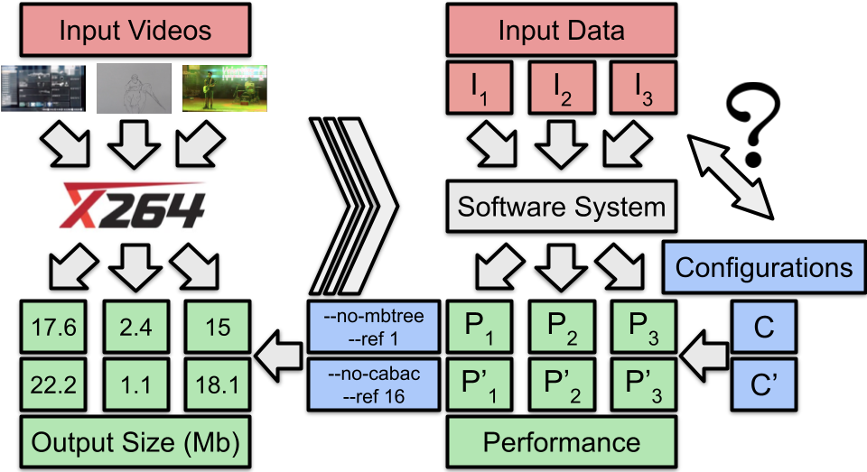
Figure 1: This paper explores and quantifies how inputs fed to software systems impact performance of configurations.

However, there exists cases where inputs (e.g., files fed to an archiver like xz or SAT formulae provided as input to a solver like lingeling) can also impact software variability [105, 54]. The x264 encoder typifies this problem, as illustrated in Figure 1. For example, Kate, an engineer working for a VOD company, wants x264 to compress input videos to the smallest possible size. She executes x264 with two configurations C (with options --no-mbtree --ref $1$) and C’ (with options --no-cabac --ref $16$) on the input video $I_{1}$ and states that C is more appropriate than C’ in this case. But when trying it on a second input video $I_{2}$, she draws opposite conclusions; for $I_{2}$, C’ leads to a smaller output size than C. Now, Kate wonders what configuration to choose for other inputs, C or C’? More generally, do configuration options have the same effect on the output size despite a different input? Do options interact in the same way no matter the inputs? These are crucial practical issues: the diversity of existing inputs can alter her knowledge of x264’s variability. If it does, Kate would have to configure x264 as many times as there are inputs, making her work really tedious and difficult to automate for a field deployment.

Numerous research works have proposed to model performance of software configurations, with several use-cases in mind for developers and users of software systems: the maintenance and understanding of configuration options and their interactions [83], the selection of an optimal configuration (tuning) [70, 25, 67], the performance prediction of arbitrary configurations [5, 44, 72] or the automated specialization of configurable systems [93, 92]. These works measure the performance of several configurations (a sample) under specific settings to then build a performance model. Input data further challenges these use-cases, since both the software configuration and the input spaces should be handled. Inputs also question and can threaten the generalization of configuration knowledge e.g., a performance prediction model for a given input may well be meaningless and inaccurate for another input.

On the one hand, some works have been addressing the performance analysis of software systems [76, 12, 23, 27, 53, 86] depending on different input data (also called workloads or benchmarks), but all of them only considered a rather limited set of configurations. On the other hand, works and studies on configurable systems usually neglect input data (e.g., using a unique video for measuring the configurations of a video encoder). We aim to combine both dimensions by performing an in-depth, controlled study of several configurable systems to make it vary in the large, both in terms of configurations and inputs. In contrast to research papers mixing multiple factors of the executing environment [42, 98], we concentrate on inputs and software configurations only, which allow us to draw reliable conclusions regarding the specific impact of inputs on software variability.

In this paper, we conduct, to our best knowledge, the first in-depth empirical study that measures how inputs individually interacts with software variability. To do so, we systematically explore the impact of inputs and configuration options on the performance properties of $8$ software systems. This study reveals that inputs fed to software systems can indeed interact with their options in non-monotonous ways, thus significantly impacting their performance properties. This observation questions the applicability of performance predictive models trained on only one input: are they still useful for other inputs? We then survey state-of-the-art papers on configurable systems to assess whether they address this kind of input sensitivity issue. Our contributions are as follows:

• To our best knowledge, the first in-depth empirical study that investigates the interactions between input data and configurations of $8$ software systems over $1\,976\,025$ measurements;

• We show that inputs fed to software systems can interact with their configuration options in non monotonous ways, thus changing performance of software systems and making it difficult to (automatically) configure them;

• The quantification of input sensitivity through several indicators and metrics per system and performance property;

• An analysis of how $65$ state-of-the-art research papers on configurable systems address this problem in practice;

• A discussion on the impacts of our study (including key insights and open problems) for different engineering tasks of configurable systems (tuning, prediction, understanding, testing, etc.);

• Open science: a replication bundle that contains docker images, produced datasets of measurements and code.

The remainder of this paper is organized as follows: Section 2 explains the problem of input sensitivity and the research questions addressed in this paper. Section 3 presents the experimental protocol. Section 4 details the results. Section 5 shows how researchers address input sensitivity. Section 6 discusses the implications of our work. Section 7 details threats to validity. Section 9 summarizes key insights of our paper.

Typographic Convention. For this paper, we adopt the following typographic convention: emphasized will be relative to a software system, slanted to its configuration options and underlined to its performance properties.

2 Problem Statement

2.1 Sensitivity to Inputs of Configurable Systems

Configuration options of software systems can have different effects on performance (e.g., runtime), but so can the input data. For example, a configurable video encoder like x264 can process many kinds of inputs (videos) in addition to offering options on how to encode. Our hypothesis is that there is an interplay between configuration options and input data: some (combinations of) options may have different effects on performance depending on input.

Researchers observed input sensitivity in multiple fields, such as SAT solvers [105, 22], compilation [74, 16], video encoding [61], data compression [47]. However, existing studies either consider a limited set of configurations (e.g., only default configurations), a limited set of performance properties, or a limited set of inputs [1, 76, 12, 23, 27, 53, 86]. It limits some key insights about the input sensitivity of configurable systems. Valov et al. [98] studied the impact of hardware on software configurations, but fixed the input fed to software systems. Jamshidi et al. [41] explored how environmental conditions (hardware, input, and software versions) impact performances of software configurations. Besides considering a limited set of inputs (e.g., 3 input videos for x264), their study did not aim to isolate the individual effects of input data on software configurations. As a result, it is impossible to draw reliable conclusions about the specific variability factors – among hardware, inputs and versions.

This work details, to the best of our knowledge, the first systematic empirical study that analyzes the interactions between input data and configuration options for different configurable systems. Through four research questions introduced in the next section, we characterise the input sensitivity problem and explore how this can alter our understanding of software variability.

2.2 Research Questions

When a developer provides a default configuration for its software system, one should ensure it will perform at best for a large panel of inputs. That is, this configuration will be near-optimal whatever the input. Hence, a hidden assumption is that two performance distributions over two different inputs are somehow related and close. In its simplest form, there could be a linear relationship between these two distributions: they simply increase or decrease with each other. RQ₁ - To what extent are the performance distributions of configurable systems changing with input data? To answer this, we compute and compare performance distributions of different inputs. For software systems, unstable performance distributions across inputs induce that their optimal configuration change with their inputs. In particular, the default configuration should be adapted according to their input data.

But configuration options influence software performance, e.g., the energy consumption [13]. An option is called influential for a performance when its values have a strong effect on this performance [42, 18]. For example, developers might wonder whether the option they add to a configurable system has an influence on its performance. However, is an option identified as influential for some inputs still influential for other inputs? If not, it would become both tedious and time-consuming to find influential options on a per-input basis. Besides, it is unclear whether activating an option is always worth it in terms of performance; an option could improve the overall performance while reducing it for few inputs. If so, users may wonder which options to enable to improve software performance based on their input data. RQ₂ - To what extent the effects of configuration options are consistent with input data? In this question, we quantify how the effects and importance of software options change with input data. If this change is significant, tuning these options to optimize performance should be adapted to the current input.

$RQ_{1}$ and $RQ_{2}$ study how inputs affect (1) performance distributions and (2) the effects of different configuration options. However, the performance distributions could change in a negligible way, without affecting the software user’s experience. Before concluding on the real impact of the input sensitivity, it is necessary to quantify how much this performance changes from one input to another. RQ₃ - How much performance are lost when reusing a configuration across inputs? In particular, we estimate the loss in performance when configuring a software while ignoring the input sensitivity to inputs. To put it more positively, this loss is also the potential gain, in terms of performance, to tune a software system for its input data.

$RQ_{1}$ to $RQ_{3}$ present the problem of input sensitivity. The fourth and last question explores the limits of this problem and give insights on how to address it concretely. Though all inputs are different, the number of possible interactions between the software systems and the processed inputs is limited. Therefore, there might exist inputs interacting in the same way with the software, and thus having similar performance profiles. RQ₄ - What is the benefit of grouping the inputs? For this question, we form, analyze and characterize different groups of inputs having similar performance distributions and show the benefits of these groups to address the input sensitivity issue.

3 Experimental protocol

We designed the following experimental protocol to answer these research questions.

Table 1: Subject Systems. See Figure 2 for notations.

System	Domain	Commit	#LoCs	Configs #C	Inputs I	#I	#M	Performance(s) P	Docker	Dataset
gcc	Compilation	ccb4e07	$9\,606\,697$	$80$	.c programs	$30$	$2400$	size, ctime, exec	Link	Link
ImageMagick	Image processing	5ee49d6	$648\,984$	$100$	images	$1000$	$100\,000$	size, time	Link	Link
lingeling	SAT solver	7d5db72	$33\,402$	$100$	SAT formulae	$351$	$35\,100$	#confl.,#reduc.	Link	Link
nodeJS	JS runtime env.	78343bb	$6\,205\,618$	$50$	.js scripts	$1939$	$96\,950$	#operations/s	Link	Link
poppler	PDF rendering	42dde68	$197\,019$	$16$	.pdf files	$1480$	$23\,680$	size, time	Link	Link
SQLite	DBMS	53fa025	$320\,049$	$50$	databases	$150$	$7500$	$15$ query times q$1$-q$15$	Link	Link
x264	Video encoding	e9a5903	$110\,642$	$201$	videos	$1397$	$280\,797$	cpu, fps, kbs, size, time	Link	Link
xz	Data compression	e7da44d	$37\,489$	$30$	system files	$48$	$1440$	size, time	Link	Link

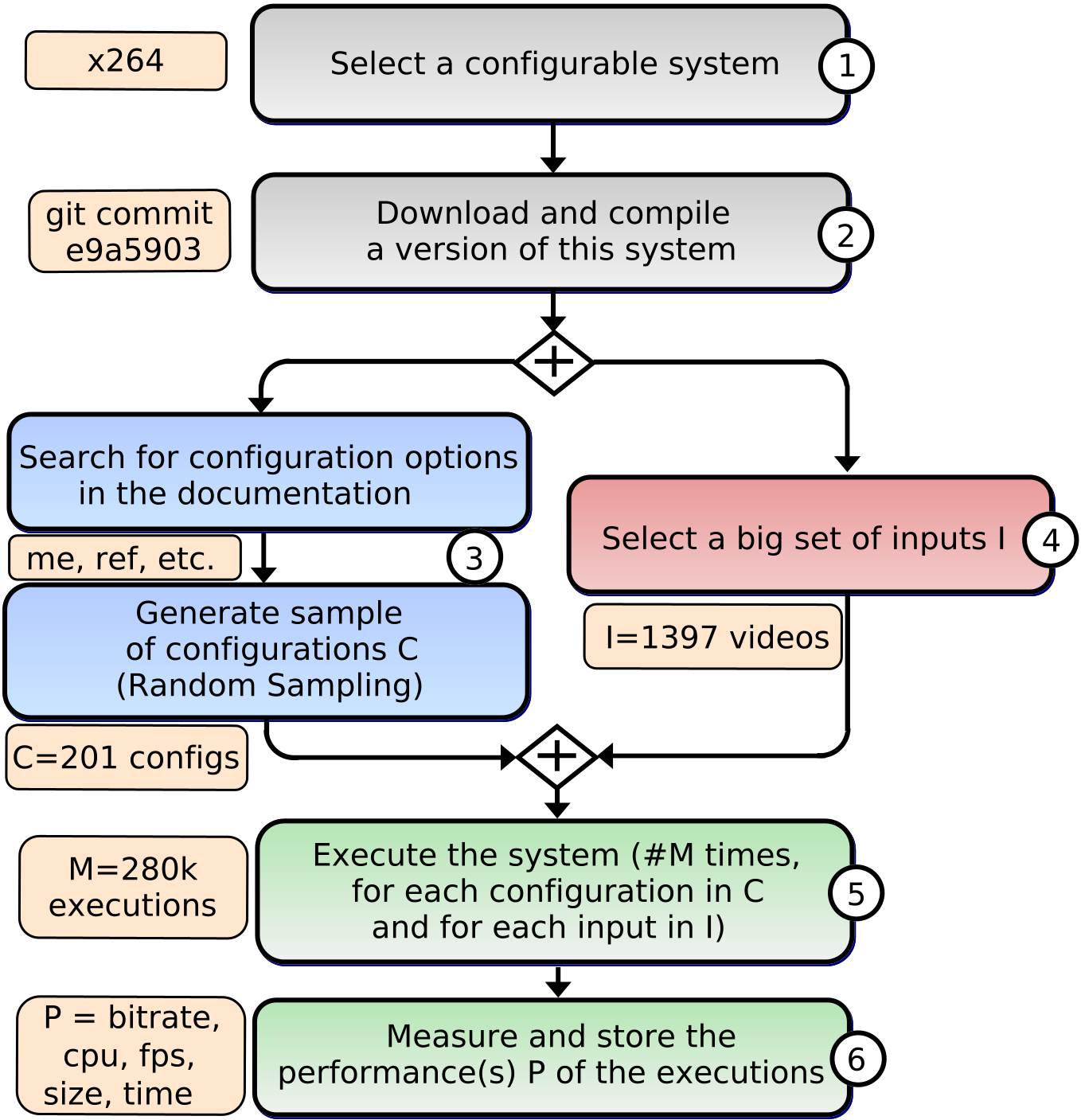
Figure 2: Measuring performance - Protocol

3.1 Data Collection

We first collect measurements of systems processing inputs.

Protocol. Figure 2 depicts the step-by-step protocol we respect to measure performance of software systems. Each line of Table 1 should be read following Figure 2: System with Steps $1$ and $2$; Configurations #C with Step $3$; the nature of inputs I and their number #I with Step $4$; Performance P with Steps $5$ and $6$; Docker links a container for executing all the steps and Data the datasets containing the performance measurements. Figure 2 shows in beige an example with the x264 encoder. Hereafter, we provide details for each step of the protocol.

Steps 1 & 2 - Software Systems. We consider $8$ software systems. We choose them because they are open-source, well-known in various fields and already studied in the literature: gcc [74, 10], the compiler for gnu operating system; ImageMagick [88, 87], a software system processing pictures and images; lingeling [36, 22], a SAT solver; nodeJS [38, 89], a widely-used JavaScript execution environment; poppler [48, 58], a library designed to process .pdf files; SQLite [92, 41], a database manager system; x264 [41, 5], a video encoder based on H264 specifications; xz [98, 64], a file system manager. We also choose these systems because they handle different types of input data, allowing us to draw conclusions as general as possible. For each software system, we use a unique private server with the same configuration running over the same operating system. We download and compile a unique version of the system. All performance are measured with this version of the software.

Step 3 - Configuration options C. To select the configuration options, we read the documentation of each system and manually extract the options affecting the performance of the system. For instance, according to the documentation of x264, the option --mbtree ”can lead to large savings for very flat content” and ”animated content should use stronger --deblock settings”. Out of these configuration options, we then sample #C configurations by using random sampling [73]. In the previous example, after the selection of --mbtree and --deblock, the sampling step would generate multiple configurations with combinations of options’ values: $C_{1}$, with --mbtree activated and --deblock set to ”0:0”; $C_{2}$, with --mbtree deactivated and --deblock set to ”-2:-2”; $C_{3}$, with --mbtree deactivated and --deblock set to ”0:0”. To ensure that each value of a software option is well represented in the final set of configurations, we statistically test the uniformity of its values. To do so, we apply a Kolmogorov-Smirnov test [60] to each option of our eight software systems. In the previous example, for a boolean option like --mbtree that can be either activated or deactivated, a valid Kolmogorov-Smirnov test guarantees that --mbtree is activated in roughly $50\text{\,}\mathrm{\char 37\relax}$ of the configurations. To mitigate the threat of only using random sampling, we also considered various informed configurations picked in the documentation. For instance, for x264, we considered the ten presets configurations recommended by the documentation

Step 4 - Inputs I. For each system, we select a different set of input data: for gcc, PolyBench v$3.1$ [78]; for ImageMagick, a sample of ImageNet [14] images (from $1.1\text{\,}\mathrm{kB}$ to $7.3\text{\,}\mathrm{MB}$); for lingeling, the 2018 SAT competition’s benchmark [36]; for nodeJS, its test suite; for poppler, the Trent Nelson’s PDF Collection [68]; for SQLite, a set of generated TPC-H [75] databases (from $10\text{\,}\mathrm{MB}$ to $6\text{\,}\mathrm{GB}$); for x264, the YouTube User General Content dataset [101] of videos (from $2.7\text{\,}\mathrm{MB}$ to $39.7\text{\,}\mathrm{GB}$); for xz, a combination of the Silesia [15] and the Canterbury[8] corpus. We choose them because these are large and freely available datasets of inputs, well-known in their field and already used by researchers and practitioners.

Steps 5 & 6 - Performance properties P. For each system, we systematically execute all the configurations of C on all the inputs of I. For the #M resulting executions, we measure as many performance properties as possible: for gcc, ctime and exec the times needed to compile and execute a program and the size of the binary; for ImageMagick, the time to apply a Gaussian blur [37] to an image and the size of the resulting image; for lingeling, the number of conflicts and reductions found in $10$ seconds of execution; for nodeJS, the number of operations per second (ops) executed by the script; for poppler, the time needed to extract the images of the pdf, and the size of the images; for SQLite, the time needed to answer $15$ different queries q$1$ $\to$ q$15$; for x264, the bitrate (the average amount of data encoded per second), the cpu usage (percentage), the average number of frames encoded per second (fps), the size of the compressed video and the elapsed time; for xz, the size of the compressed file, and the time needed to compress it. It results in a set a tabular data, one for each input and each software system, consisting of a list of configurations with their performance property values.

Replication. To allow researchers to easily replicate the measurement process, we provide a docker container for each system (see the links in the Docker column of Table 1). We also publish the resulting datasets online (see the links in the Data column) and in the companion repository with replication details.

3.2 Performance Correlations ($RQ_{1}$)

Based on the analysis of the data collected in Section 3.1, we can now answer the first research question: RQ₁ - To what extent are the performance distributions of configurable systems changing with input data? To check this hypothesis, we compute, analyze and compare the Spearman’s rank-order correlation [46] of each couple of inputs for each system. It is appropriate in our case since all performance properties are quantitative variables measured on the same set of configurations.

Spearman correlations. The correlations are considered as a measure of similarity between the configurations’ performance over two inputs. We compute the related $p$-values: a correlation whose $p$-value is higher than the chosen threshold $0.05$ is considered as null. We use the Evans rule [21] to interpret these correlations. In absolute value, we refer to correlations by the following labels; very low: 0-0.19, low: 0.2-0.39, moderate: 0.4-0.59, strong: 0.6-0.79, very strong: 0.8-1.00. A negative score tends to reverse the ranking of configurations. Very low or negative scores have practical implications: a good configuration for an input can very well exhibit bad performance for another input.

3.3 Effects of Options ($RQ_{2}$)

To understand how a performance model can change based on a given input, we next study how input data interact with configuration options. RQ₂ - To what extent the effects of configuration options are consistent with input data? To assess the relative significance and effect of options, we use two well-known statistical methods [81, 9], also widely used in the context of interpretable machine learning and configurable systems [72, 62, 41]. For instance, Jamshidi et al. [41] used similar indicators to measure the sensitivity of configurations regarding computing environmental conditions (hardware, input, and software versions).

Random forest importances. The tree structure provides insights about the most essential options for prediction, because such a tree first splits w.r.t. options that provide the highest information gain. We use random forests [9], a vote between multiple decision trees: we can derive, from the forests trained on the inputs, estimates of the options importance. The computation of option importance is realized through the observation of the effect on random forest accuracy when randomly shuffling each predictor variable [62]. For a random forest, we consider that an option is influential if the median (on all inputs) of its option importance is greater than $\frac{1}{n_{opt}}$, where $n_{opt}$ is the number of options considered in the dataset. This threshold represents the theoretic importance of options for a software having equally important options.

Linear regression coefficients. The coefficients of an ordinary least square regression [81] weight the effect of configuration options. These coefficients can be positive (resp. negative) if a bigger (resp. lower) option value results in a bigger performance. Ideally, the sign of the coefficients of a given option should remain the same for all inputs: it would suggest that the effect of an option onto performance is stable. We also provide details about coefficients related to feature interactions [96, 80] in the companion repository.

3.4 Impact of Inputs on Performance ($RQ_{3}$)

To complete this experimental protocol, we ask whether adapting the software to its input data is worth the cost of finding the right set of parameters i.e., the concrete impact of input sensitivity. RQ₃ - How much performance are lost when reusing a configuration across inputs? To estimate how much we can lose, we first define two scenarios of reuse $S_{1}$ and $S_{2}$:

1. Baseline. In this scenario, we value input sensitivity and just train a simple performance model on a target input. We choose the best configuration according to the model, configure the related software with it and execute it on the target input.

2. Ignoring input sensitivity. In this scenario, let us pretend that we ignore the input sensitivity issue. We train a model related to a given input i.e., the source input, and then predict the best configuration for this source input. If we ignore the issue of input sensitivity, we should be able to easily reuse this model for any other input, including the target input of $S_{1}$. Finally, we execute the software with the predicted configuration on the target input.

In this part, we systematically compare $S_{1}$ and $S_{2}$ in terms of performance for all inputs, all performance properties and all software systems. For $S_{1}$, we repeat the scenario ten times with different sources, uniformly chosen among other inputs and compute the average performance. For both scenarios, due to the imprecision of the learning procedure, the models can recommend sub-optimal configurations. Since this imprecision can alter the results, we consider an ideal case for both scenarios and assume that the performance models always recommend the best possible configuration.

Performance ratio. To compare $S_{1}$ and $S_{2}$, we use a performance ratio i.e., the performance obtained in $S_{1}$ over the performance obtained in $S_{2}$. If the ratio is equal to $1$, there is no difference between $S_{1}$ and $S_{2}$ and the input sensitivity does not exist. A ratio of $1.4$ would suggest that the performance of $S_{1}$ is worth $1.4$ times the performance of $S_{2}$; therefore, it is possible to gain up to $(1.4-1)*100=40\%$ performance by choosing $S_{1}$ instead of $S_{2}$. We also report on the standard deviation of the performance ratio distribution. A standard deviation of 0 implies that we gain or lose the same proportion of performance when picking $S_{1}$ over $S_{2}$.

3.5 Groups of Inputs ($RQ_{4}$)

Lastly, we explore how the issue of input sensitivity can be concretely addressed. For mitigating input sensitivity, an idea is to group together inputs based on their performance distributions. RQ₄ - What is the benefit of grouping the inputs? The inputs belonging to the same group are supposed to share common properties and be processed in a similar manner by the software [16]. We perform hierarchical clustering [69] to gather inputs having similar performance profiles.

Hierarchical clustering. This technique considers the correlations between performance distributions as a measure of similarity between inputs. Based on these values, it forms groups of inputs minimizing the intra-class variance ( discrepancy of performance among a group) and maximizing the inter-class variance (discrepancy of performance between different groups of inputs). As linkage criteria, we choose the Ward method [69] since in our case, (1) single link (minimum of distance) leads to numerous tiny groups (2) centroid or average tend to split homogeneous groups of inputs and (3) complete link aggregates unbalanced groups. As a metric, we kept the Euclidian distance - used as default. We manually select the final number of groups.

For each group, we then report on few key indicators summarizing the specifics of inputs’ performance: the Spearman correlations between performance distributions of inputs ($RQ_{1}$), the importance and effects of options ($RQ_{2}$) as well as few properties characterizing the inputs e.g., the spatial complexity of an input video or the number of lines of a .c program. We compare their average value in the different groups.

4 Results

4.1 Performance Correlations ($RQ_{1}$)

We first explain the results of $RQ_{1}$ and their consequences on the poppler use case i.e., an extreme case of input sensitivity, and then generalize to our other software systems.

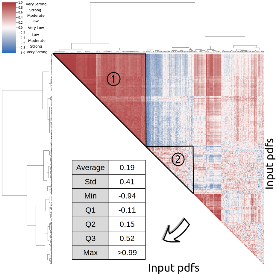
Each square_(i,j) represents the Spearman correlation between the time needed to extract the images of pdfs $i$ and $j$. The color of this square respects the top-left scale: high positive correlations are red; low in white; negative in blue. Because we cannot describe each correlation individually, we added a table describing their distribution.

Figure 3: Spearman rank based correlations - poppler, time.

Extract images of input pdfs with poppler. The content of pdf files fed to poppler may vary; the input pdf can contain a $2$-page extended abstract with plain text, a $10$-page conference article with few figures or a $300$-page book full of pictures. Depending on this content, extracting the images embedded in those files can be quicker or slower for the same configuration. Moreover, different configurations could be adapted for the conference paper but not for the book (or conversely), leading to different rankings of extraction time and thus different rank-based correlation values.

Figure 3 depicts the Spearman rank-order correlations of extraction time between pairs of input pdfs fed to poppler. Results suggest a positive correlation (see dark red cells), though there are pairs of inputs with lower (see white cells) and even negative (see dark blue cells) correlations. More than a quarter of the correlations between input pdfs are positive and at least moderate - third quartile Q3 greater than $0.52$.

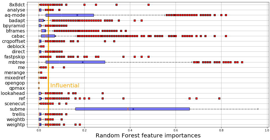
((a)) Importance

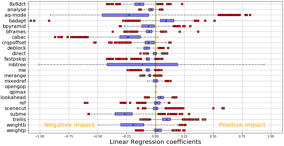
((b)) Effect

Figure 4: Importance and effect (x-axis) of configuration options (y-axis) - x264, bitrate

Meta-analysis. Over the $8$ systems, we observe different cases. There exist software systems not sensitive at all to inputs. In our experiment, gcc, imagemagick and xz present almost exclusively high and positive correlations between inputs e.g., Q1 = $0.82$ for the compressed size and xz. For these, un- or negatively-correlated inputs are an exception more than a rule. In contrast, there are software systems, namely lingeling, nodeJS, SQLite and poppler, for which performance distributions completely change and depend on input data e.g., Q2 = $0.09$ for nodeJS and ops, Q3 = $0.12$ for lingeling and conflicts. For these, we draw similar conclusions as in the poppler case. In between, x264 is only input-sensitive w.r.t. a performance property; it is for bitrate and size but not for cpu, fps and time e.g., $0.29$ as deviation for size against $0.08$ for time.

4.2 Effects of Options ($RQ_{2}$)

We first explain the results of $RQ_{2}$ and their concrete consequences on the bitrate of x264 - an input-sensitive case, to then generalize to other software systems.

Encoding input videos with x264. Figures 4(a) and 4(b) report on respectively the boxplots of configuration options’ feature importances and effects when predicting x264’s bitrate for all input videos. On the top graph, we displayed the boxplots of the distribution of importances for each option (y-axis). On the bottom graph, we displayed the boxplots of the distribution of regression coefficients for each option (y-axis). Each red square is representing a model trained on one input, and all of them constitute the resulting distribution. Each algorithm is using $100\text{\,}\mathrm{\char 37\relax}$ of the configurations in the training set. We also compute the Mean Absolute Percentage Error (MAPE) for all the systems, inputs and non functional properties when predicting the performance with random forests and linear regression. For random forest, we can ensure that our models are giving a good prediction, the median value of the MAPE across all inputs being systematically under $5\text{\,}\mathrm{\char 37\relax}$ for each couple of software systems and performance properties. For Linear Regression, results tend to show higher values of MAPE, suggesting that the configurations spaces are too hard to learn from for such simple models. Other variants of feature importances and linear regression (permutation importance, drop-column importance and Shapley values) have been computed to ensure the robustness of results in the companion repository. They reached similar results, which confirms our conclusions with the chosen indicators.

Three options are strongly influential for a majority of videos on Figure 4(a): subme, mbtree and aq-mode, but their importance can differ depending on input videos: for instance, the importance of subme is $0.83$ for video #$1365$ and only $0.01$ for video #$40$. Because influential options vary with inputs, performance models and approaches based on feature selection [62] such as performance-influence model [83, 102] may not generalize well to all input videos.

Most of the options have positive and negative coefficients on Figure 4(b); thus, the specific effects of options heavily depend on input videos. It is also true for influential options: mbtree can have positive and negative (influential) effects on the bitrate i.e., activating mbtree may be worth only for few input videos. The consequence is that tuning the options of a software system should be adapted to the current input, and not done once for all the inputs.

Meta-analysis. For gcc, imagemagick and xz, the importances are quite stable. As an extreme case of stability, the importances of the compressed size for xz are exactly the same, except for two inputs. For these systems, the coefficients of linear regression mostly keep the same sign across inputs i.e., the effects of options do not change with inputs. For input-sensitive software systems, we always observe high variations of options’ effects (lingeling, poppler or SQLite), sometimes coupled to high variations of options’ importances (nodeJS). For instance, the option format for poppler can have an importance of $0$ or $1$ depending on the input. For all software systems, there exists at least one performance property whose effects are not stable for all inputs e.g., one input with negative coefficient and another with a positive coefficient. For x264, it depends on the performance property; for cpu, fps and time, the effect of influential options are stable for all inputs, while for the bitrate and the size, we can draw the conclusions previously presented.

4.3 Impact of Inputs on Performance ($RQ_{3}$)

This section presents the evaluation of $RQ_{3}$ w.r.t. the protocol of Section 3.4. Figure 5 presents the loss of performance (y-axis, in %) due to input sensitivity for the different software systems and their performance properties.

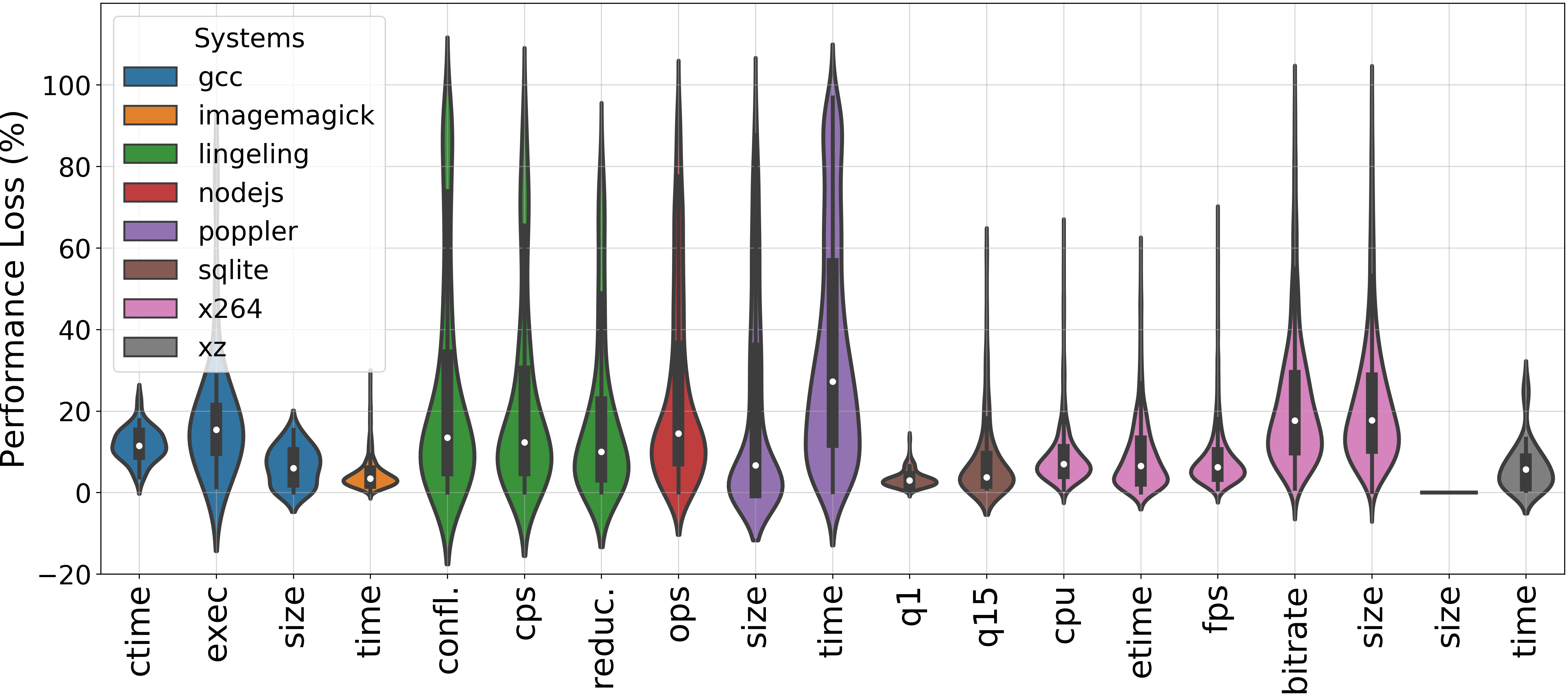
Figure 5: Performance loss (%, y-axis) when ignoring input sensitivity per system and performance property (x-axis)

Key result. The average performance ratio across all the software systems is $1.38$: we can expect an average drop of $38\text{\,}\mathrm{\char 37\relax}$ in terms of performance when ignoring the input sensitivity.

Meta-analysis. For software systems whose performance are stable across inputs (gcc, imagemagick and xz), there are few differences between inputs. For instance, for the output size of xz, there is no variation between scenarios $S_{1}$ (i.e., using the best configuration) and $S_{2}$ (i.e., reusing a the best configuration of a given input for another input): all performance ratios (i.e., performance $S_{1}$ over performance $S_{2}$) are equals to $1$ whatever the input.

For input-sensitive software systems (lingeling, nodeJS, SQLite and poppler), changing the configuration can lead to a negligible change in a few cases. For instance, for the time to answer the first query q1 with SQLite, the median is $1.03$; in this case, SQLite is sensitive to inputs, but its variations of performance -less than $4\text{\,}\mathrm{\char 37\relax}$- do not justify the complexity of tuning the software. But it can also be a huge change; for lingeling and solved conflicts, the $95^{th}$ percentile ratio is equal to $8.05$ i.e., a factor of $8$ between $S_{1}$ and $S_{2}$. It goes up to a ratio of $10.11$ for poppler’s extraction time: there exists an input pdf for which extracting its images is ten times slower when reusing a configuration compared to the fastest.

In between, x264 is a complex case. For its low input-sensitive performance (e.g., cpu and etime), it moderately impacts the performance when reusing a configuration from one input to another - average ratios at resp. $1.42$ and $1.43$. In this case, the rankings of performance do not change a lot with inputs, but a small ranking change does make the difference in terms of performance.

On the contrary, for the input-sensitive performance (e.g., the bitrate), there are few variations of performance: we can lose $1-\frac{1}{1.11}\simeq$ $9\text{\,}\mathrm{\char 37\relax}$ of bitrate in average. In this case, it is up to the compression experts to decide; if losing up to $1-\frac{1}{1.32}\simeq$ $24\text{\,}\mathrm{\char 37\relax}$ of bitrate is acceptable, then we can ignore input sensitivity. Otherwise, we should consider tuning x264 for its input video.

4.4 Groups of Inputs ($RQ_{4}$)

We illustrate the results of this section using the bitrate of x264 when encoding input videos. In Figure 6, we first compute the correlations between performance of all input videos, as in $RQ_{1}$. Then, we perform hierarchical clustering on x264 measurements to gather inputs having similar bitrate distributions and visually group correlated videos together. The resulting groups are delimited and numbered directly in the figure. For instance, the group \raisebox{-.9pt} {1}⃝ is located in the top-left part of the correlogram by the triangle \raisebox{-.9pt} {1}⃝).

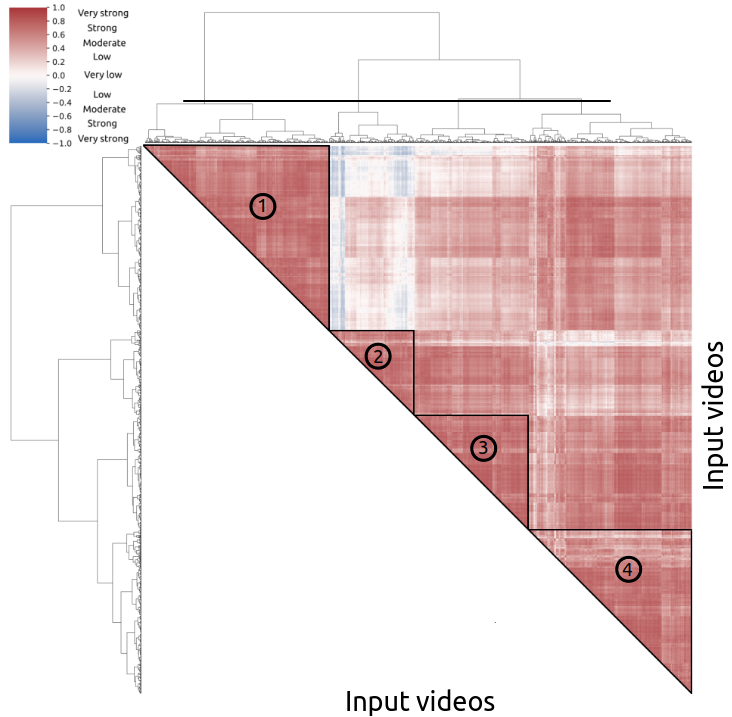
Figure 6: Performance groups of input videos - x264, bitrate

Table 2: Performance groups of input videos - x264, bitrate

Group		\raisebox{-.9pt} {1}⃝ Action	\raisebox{-.9pt} {2}⃝ Big	\raisebox{-.9pt} {3}⃝ Still image	\raisebox{-.9pt} {4}⃝ Standard
# Inputs		470	219	292	416
Input Properties		Spatial ++	Spatial ––	Spatial ––	Width -
		Chunk ++	Temporal ++	Temporal ––	Height -
			Width ++	Chunk ––	Temporal -
Main Category		Sports	HDR	Lecture	Music
		News		HowTo	Vertical
Avg Correlation		0.82 $\pm$ 0.11	0.79 $\pm$ 0.14	0.85 $\pm$ 0.09	0.74 $\pm$ 0.17
(e.g., fig. 3)
Imp.	––mbtree	0.09 $\pm$ 0.09	0.47 $\pm$ 0.2	0.34 $\pm$ 0.22	0.05 $\pm$ 0.07
(fig. 4(a))	––aq-mode	0.27 $\pm$ 0.19	0.13 $\pm$ 0.13	0.04 $\pm$ 0.07	0.15 $\pm$ 0.18
Effect	––mbtree	0.33 $\pm$ 0.19	-0.68 $\pm$ 0.18	-0.42 $\pm$ 0.15	-0.11 $\pm$ 0.15
(fig. 4(b))	––aq-mode	-0.5 $\pm$ 0.14	0.36 $\pm$ 0.21	-0.14 $\pm$ 0.14	-0.29 $\pm$ 0.18

Group description. In total, we isolate four groups of input videos. These groups are presented and described in Table 2:

• Group \raisebox{-.9pt} {1}⃝ is mostly composed of moving or action videos, often picked in the sports or news categories and with high spatial and chunk complexities;

• Group \raisebox{-.9pt} {2}⃝ gathers large input videos, with big resolution videos, taken for instance in the High Dynamic Range category. They typically have a low spatial complexity and a high temporal complexity;

• Group \raisebox{-.9pt} {3}⃝ is composed of ”still image” videos i.e., input videos with few changes of background, with low temporal and chunk complexities. A typical example of this kind of video would be a course with a fixed board, chosen in the Lecture or in the HowTo category;

• Group \raisebox{-.9pt} {4}⃝ is a group of average videos with average properties values and various contents.

Revisiting $RQ_{1}$. In a group of inputs, performance distributions of inputs are highly correlated with each other - positively, strong or very strong. The input videos of the same group have similar bitrate rankings; their performance react the same way to the same configurations of x264. However, the group \raisebox{-.9pt} {1}⃝ is uncorrelated (very low, low) or negatively correlated (moderate, strong and very strong) with the group \raisebox{-.9pt} {2}⃝ - see the intersection area between triangles \raisebox{-.9pt} {1}⃝ and \raisebox{-.9pt} {2}⃝. In this case, a single configuration of x264 working for the group \raisebox{-.9pt} {1}⃝ should not be reused directly on a video of the group \raisebox{-.9pt} {2}⃝. So, these groups are capturing the difference of performance between inputs; once in a group, input sensitivity does not represent a problem anymore.

Revisiting $RQ_{2}$. Within a group, the effect and importance of options are stable and the inputs all react the same way to the same options, while they differ between the different groups. For instance, for the group \raisebox{-.9pt} {1}⃝, aq-mode is influential (Imp = $0.27$), while it is not for the group \raisebox{-.9pt} {3}⃝ (Imp = $0.04$). Likewise, the effects of mbtree vary with the group of inputs; for the group \raisebox{-.9pt} {1}⃝, activating mbtree always increases the bitrate (Effect = +$0.33$), while for the groups \raisebox{-.9pt} {2}⃝, \raisebox{-.9pt} {3}⃝ and \raisebox{-.9pt} {4}⃝, it diminishes the bitrate (Effects = -$0.68$, -$0.42$, -$0.11$ respectively). Under these circumstances, configuring the software system once per group of inputs is probably a reasonable solution for tackling input sensitivity.

Revisiting $RQ_{3}$. For the bitrate of x264, reusing a configuration from a source input to a target input generate a lower performance drop if the source and the target inputs are selected in the same group (e.g., $13\text{\,}\mathrm{\char 37\relax}$ for group 2) compared to a random selection ($34\text{\,}\mathrm{\char 37\relax}$ in general). If we are able to find the best configuration for one input video in a group, this configuration will be good-enough for the rest of the inputs in this group.

Meta-analysis. For the other input-sensitive systems, results tend to show similar results as for x264 and the bitrate. For instance, with poppler, grouping tend to gather inputs with the same influence and effect of options; for the size, the importance of format is influential in groups 2 and 4 but not in groups 1 and 3; for the execution time, in groups 1 and 2, -jp2 has a positive effect overall while a negative effect for groups 3 and 4. When the groups discriminate inputs with different effects of options, $RQ_{3}$ results tend to be more impressive e.g., the average performance loss of $49\text{\,}\mathrm{\char 37\relax}$ vanishes when grouping the inputs (in the four groups, $1\text{\,}\mathrm{\char 37\relax}$-$4\text{\,}\mathrm{\char 37\relax}$-$12\text{\,}\mathrm{\char 37\relax}$-$2\text{\,}\mathrm{\char 37\relax}$ when reusing a configuration inside the group). The same applies for Nodejs : --jitless is influential for groups 2, 3 and 4 but not for group 1. In $RQ_{3}$ results, the average performance drop of $44\text{\,}\mathrm{\char 37\relax}$ becomes $7.4\text{\,}\mathrm{\char 37\relax}$-$6.7\text{\,}\mathrm{\char 37\relax}$-$13.7\text{\,}\mathrm{\char 37\relax}$-$9.0\text{\,}\mathrm{\char 37\relax}$ in the four groups. For non input-sensitive systems, we do not observe such difference between the groups. Grouping seems to be ineffective; the same effect of options are observed; it does not change the performance loss, already low e.g., for the execution time of imagemagick, $6\text{\,}\mathrm{\char 37\relax}$ in general and $1\text{\,}\mathrm{\char 37\relax}$-$1\text{\,}\mathrm{\char 37\relax}$-$2\text{\,}\mathrm{\char 37\relax}$-$6\text{\,}\mathrm{\char 37\relax}$ in the groups.

Classify inputs into groups. In short, grouping together inputs seems a right approach to reduce input sensitivity. However there is now a problem: we need to map a given input into a group a priori, without having access to all measurements. Since these four groups are consistent and share common properties, one domain expert or one machine learning model could classify these inputs a priori into a group without measuring their performance just by looking at the properties of the inputs.

Benefits for benchmarking. These groups allow to increase the representativeness of profiles of inputs used to test software systems, while greatly lowering the number of inputs of this set. In the companion repository, we operate on previous results to create a short but representative set of input videos dedicated to the benchmarking of x264: we reduce the dataset, initially composed of $1397$ input videos [101], to a subset of $8$ videos, selecting $2$ cheap videos in each group of performance.

5 Sensitivity to Inputs in Research

Table 3: Input sensitivity in research. Q-A. Is there a software system processing input data in the study? Q-B. Does the experimental protocol include several inputs? Q-C. Is the problem of input sensitivity mentioned in the paper? Q-D. Does the paper propose a solution to generalize the performance model across inputs?  Justifications in the companion repository.

ID	Authors	Conference	Year	Title	Q-A	Q-B	Q-C	Q-D
1	Guo et al. [31]	ESE	2017	Data-efficient performance learning for configurable systems	X
2	Jamshidi et al. [43]	SEAMS	2017	Transfer learning for improving model predictions […]	X	X	X
3	Jamshidi et al. [41]	ASE	2017	Transfer learning for performance modeling of configurable […]	X	X	X	X
4	Oh et al. [70]	ESEC/FSE	2017	Finding near-optimal configurations in product lines by […]	X
5	Kolesnikov et al. [49]	SoSyM	2018	Tradeoffs in modeling performance of highly configurable […]	X
6	Nair et al. [65]	ESEC/FSE	2017	Using bad learners to find good configurations	X	X
7	Nair et al. [67]	TSE	2018	Finding Faster Configurations using FLASH	X	X	X
8	Murwantara et al. [63]	iiWAS	2014	Measuring Energy Consumption for Web Service Product […]	X	X	X	X
9	Temple et al. [94]	SPLC	2016	Using Machine Learning to Infer Constraints for Product Lines
10	Temple et al. [92]	IEEE Soft.	2017	Learning Contextual-Variability Models	X		X
11	Valov et al. [98]	ICPE	2017	Transferring performance prediction models across different […]	X		X	X
12	Weckesser et al. [103]	SPLC	2018	Optimal reconfiguration of dynamic software product […]
13	Acher et al. [2]	VaMoS	2018	VaryLATEX: Learning Paper Variants That Meet Constraints	X	X
14	Sarkar et al. [80]	ASE	2015	Cost-Efficient Sampling for Performance Prediction of […]	X
15	Temple et al. [91]	Report	2018	Towards Adversarial Configurations for Software Product Lines
16	Nair et al. [66]	ASE	2018	Faster Discovery of Faster System Configurations with […]	X
17	Siegmund et al. [83]	ESEC/FSE	2015	Performance-Influence Models for Highly Configurable Systems	X
18	Valov et al. [96]	SPLC	2015	Empirical comparison of regression methods for […]	X
19	Zhang et al. [106]	ASE	2015	Performance Prediction of Configurable Software Systems […]	X		X
20	Kolesnikov et al. [50]	ESE	2019	On the relation of control-flow and performance feature […]	X
21	Couto et al. [13]	SPLC	2017	Products go Green: Worst-Case Energy Consumption […]	X		X
22	Van Aken et al. [99]	SIGMOD	2017	Automatic Database Management System Tuning Through […]	X	X	X	X
23	Kaltenecker et al. [45]	ICSE	2019	Distance-based sampling of software configuration spaces	X
24	Jamshidi et al. [42]	ESEC/FSE	2018	Learning to sample: exploiting similarities across […]	X	X	X	X
25	Jamshidi et al. [40]	MASCOTS	2016	An Uncertainty-Aware Approach to Optimal Configuration of […]	X	X	X
26	Lillacka et al. [56]	Soft. Eng.	2013	Improved prediction of non-functional properties in Software […]	X	X	X	X
27	Zuluaga et al. [108]	JMLR	2016	$\varepsilon$-pal: an active learning approach […]	X	X
28	Amand et al. [6]	VaMoS	2019	Towards Learning-Aided Configuration in 3D Printing […]	X	X	X
29	Alipourfard et al. [4]	NSDI	2017	Cherrypick: Adaptively unearthing the best cloud […]	X	X	X
30	Saleem et al. [79]	TSC	2015	Personalized Decision-Strategy based Web Service Selection […]	X	X
31	Zhang et al. [107]	SPLC	2016	A mathematical model of performance-relevant […]	X
32	Ghamizi et al. [26]	SPLC	2019	Automated Search for Configurations of Deep Neural […]	X	X	X
33	Grebhahn et al. [28]	CPE	2017	Performance-influence models of multigrid methods […]
34	Bao et al. [7]	ASE	2018	AutoConfig: Automatic Configuration Tuning for Distributed […]	X	X
35	Guo et al. [30]	ASE	2013	Variability-aware performance prediction: A statistical […]	X
36	Švogor et al. [109]	IST	2019	An extensible framework for software configuration optim[…]	X	X
37	El Afia et al. [3]	CloudTech	2018	Performance prediction using support vector machine for the […]	X	X
38	Ding et al. [16]	PLDI	2015	Autotuning algorithmic choice for input sensitivity	X	X	X	X
39	Duarte et al. [20]	SEAMS	2018	Learning Non-Deterministic Impact Models for Adaptation	X	X	X	X
40	Thornton et al. [95]	KDD	2013	Auto-WEKA: Combined selection and hyperparameter […]	X	X	X
41	Siegmund et al. [84]	ICSE	2012	Predicting performance via automated feature-inter[…]	X	X	X
42	Siegmund et al. [85]	SQJ	2012	SPL Conqueror: Toward optimization of non-functional […]	X	X
43	Westermann et al. [104]	ASE	2012	Automated inference of goal-oriented performance prediction […]	X	X
44	Velez et al. [100]	ICSE	2021	White-Box Analysis over Machine Learning: Modeling […]	X	X
45	Pereira et al. [5]	ICPE	2020	Sampling Effect on Performance Prediction of Configurable […]	X	X	X
46	Shu et al. [82]	ESEM	2020	Perf-AL: Performance prediction for configurable software […]	X
47	Dorn et al. [19]	ASE	2020	Mastering Uncertainty in Performance Estimations of […]	X
48	Kaltenecker et al. [44]	IEEE Soft.	2020	The Interplay of Sampling and Machine Learning for Software […]	X
49	Krishna et al. [51]	TSE	2020	Whence to Learn? Transferring Knowledge in Configurable […]	X	X	X	X
50	Weber et al. [102]	ICSE	2021	White-Box Performance-Influence Models: A Profiling […]	X	X
51	Mühlbauer et al. [64]	ASE	2020	Identifying Software Performance Changes Across Variants […]	X	X
52	Han et al. [34]	Report	2020	Automated Performance Tuning for Highly-Configurable […]	X	X
53	Han et al. [35]	ICPE	2021	ConfProf: White-Box Performance Profiling of Configuration […]	X		X
54	Valov et al. [97]	ICPE	2020	Transferring Pareto Frontiers across Heterogeneous Hardware […]	X			X
55	Liu et al. [57]	CF	2020	Deffe: a data-efficient framework for performance […]	X	X	X	X
56	Fu et al. [24]	NSDI	2021	On the Use of ML for Blackbox System Performance Prediction	X	X	X
57	Larsson et al. [52]	IFIP	2021	Source Selection in Transfer Learning for Improved Service […]	X	X	X	X
58	Chen et al. [10]	ICSE	2021	Efficient Compiler Autotuning via Bayesian Optimization	X	X	X
59	Chen et al. [11]	SEAMS	2019	All Versus One: An Empirical Comparison on Retrained […]	X	X
60	Ha et al. [32]	ICSE	2019	DeepPerf: Performance Prediction for Configurable Software […]	X
61	Pei et al. [71]	Report	2019	DeepXplore: automated white box testing of deep […]	X	X
62	Ha et al. [33]	ICSME	2019	Performance-Influence Model for Highly Configurable […]	X
63	Iorio et al. [39]	CloudCom	2019	Transfer Learning for Cross-Model Regression in Performance […]	X	X	X	X
64	Koc et al. [77]	ASE	2021	SATune: A Study-Driven Auto-Tuning Approach for […]	X	X	X	X
65	Ding et al. [17]	ESEC/FSE	2021	Generalizable and Interpretable Learning for […]	X	X	X	X
Total					$61$	$39$	$29$	$15$

In this section, we explore the significance of the input sensitivity problem in research. Do researchers know the issue of input sensitivity? How do they deal with inputs in their papers? Is the interaction between software configurations and input sensitivity a well-known issue?

5.1 Experimental Protocol

First, we aim at gathering research papers [29] predicting the performance of configurable systems i.e., with a performance model [30].

Gather research papers. We focused on the publications of the last ten years. To do so, we analyzed the papers published (strictly) after 2011 from the survey of Pereira et al. [72] - published in 2019. We completed those papers with more recent papers (2019-2021), following the same procedure as in [72]. We have only kept research work that trained performance models.

Search for input sensitivity. We read each selected paper and answered four different questions: Q-A. Is there a software system processing input data in the study?  If not, the impact of input sensitivity in the existing research work would be relatively low. The idea of this research question is to estimate the proportion of the performance models that could be affected by input sensitivity. Q-B. Does the experimental protocol include several inputs?  If not, it would suggest that the performance model only captures a partial truth, and might not generalize for other inputs fed to the software system. Q-C. Is the problem of input sensitivity mentioned in the paper?  This question aims to state whether researchers are aware of the input sensitivity issue, and estimate the proportion of the papers that mention it as a potential threat to validity. Q-D. Does the paper propose a solution to generalize the performance model across inputs?  Finally, we check whether the paper proposes a solution managing input sensitivity i.e., if the proposed approach could be adapted to our problem and predict a near-optimal configuration for any input. The results were obtained by one author and validated by all other co-authors.

5.2 How do Research Papers Address Input Sensitivity?

Table 3 lists the $65$ research papers we identified following this protocol, as well as their individual answers to Q-A$\to$Q-D. A checked cell indicates that the answer to the corresponding question (column) for the corresponding paper (line) is yes. Since answering Q-B, Q-C or Q-D only makes sense if Q-A is checked, we grayed and did not consider Q-B, Q-C and Q-D if the answer of Q-A is no. We also provide full references and detailed justifications in the companion repository. We now comment the average results:

Q-A. Is there a software system processing input data in the study?  Of the $65$ papers, $60$ ($94\text{\,}\mathrm{\char 37\relax}$) consider at least one configurable system processing inputs. This large proportion gives credits to input sensitivity and its potential impact on research work.

Q-B. Does the experimental protocol include several inputs?  $63\text{\,}\mathrm{\char 37\relax}$ of the research work answering yes to Q-A include different inputs in their protocol. But what about the other $37\text{\,}\mathrm{\char 37\relax}$? It is understandable not to consider several inputs because of the cost of measurements. However, if we reproduce all experiments of Table 3 using other input data, will we draw the same conclusions for each paper? Based on the results of $RQ_{1}$ $\to$ $RQ_{3}$, we encourage researchers to consider at least a set of inputs in their protocol (see Section 6).

Q-C. Is the problem of input sensitivity mentioned in the paper?  Only half ($47\text{\,}\mathrm{\char 37\relax}$) of the papers mention the issue of input sensitivity, mostly without naming it or using a domain-specific keyword e.g., workload variation [98]. For the other half, we cannot guarantee with certainty that input sensitivity concerns all papers. But we shed light on this issue: ignoring input sensitivity can prevent the generalization of performance models across inputs. This is especially true for the $37\text{\,}\mathrm{\char 37\relax}$ of papers answering no to Q-B i.e., considering one input per system: only $14\text{\,}\mathrm{\char 37\relax}$ of these research works mention it.

Q-D. Does the paper propose a solution to generalize the performance model across inputs?  We identified $15$ papers [99, 16, 20, 77, 41, 98, 42, 51, 97, 52, 39, 63, 56, 57, 17] proposing contributions that may help in better managing the input sensitivity problem. However, most of them have not been designed to operate over actual inputs, but rather changes of computing environments [41, 98, 42, 51, 97, 52, 39]. Other works [99, 16, 20, 77, 57] only apply it to a specific domain (database [99], compilation [16], cloud computing [20, 57, 17] or programs analysis [77]) with open questions about applicability and effectiveness in other areas. We plan to confront these techniques on our dataset for multiple systems.

6 Implications of our study

In this section, we first summarize results of our study and then discuss their impacts on several research directions.

Table 4: Summary of the input sensitivity on our dataset

System	Perf.	Correlation	Most infl. opt.	Impact (%)	IS
		[$C_{min}$, $C_{max}$]	Effect [min, max]	$100*(Q_{2}-1)$	Score
					(0$\to$1)
		($RQ_{1}$)	($RQ_{2}$)	($RQ_{3}$)	($RQ_{4}$)
gcc	ctime	[$0.72$, $0.97$]	[$-0.26$, $-0.18$]	$13$	0.32
	exec	[$-0.69$, $1$]	[$-0.21$, $0.64$]	$27$	0.92
	size	[$0.48$, $1$]	[$-0.03$, $0$]	$7$	0.27
image	time	[$-0.24$, $1$]	[$-0.18$, $0.95$]	$4$	0.39
lingeling	# conf	[$-0.9$, $0.92$]	[$-0.79$, $0.91$]	$15$	0.75
	# reduc	[$-0.99$, $1$]	[$-0.79$, $0.91$]	$10$	0.7
nodejs	ops	[$-0.87$, $0.95$]	[$-1<$, $0.93$]	$17$	0.79
poppler	size	[$-1$, $1$]	[$-1<$, $>1$]	$7$	0.64
	time	[$-0.94$, $1$]	[$-0.93$, $>1$]	$37$	0.98
SQLite	q1	[$-0.78$, $0.87$]	[$-0.69$, $0.58$]	$2$	0.45
	q15	[$-0.3$, $0.94$]	[$-0.59$, $0.6$]	$3$	0.37
x264	bitrate	[$-0.69$, $1$]	[$-0.55$, $0.28$]	$21$	0.84
	cpu	[$-0.31$, $1$]	[$-0.1$, $0.84$]	$7$	0.47
	fps	[$0.01$, $1$]	[$-0.62$, $0.23$]	$6$	0.37
	size	[$-0.69$, $1$]	[$-0.58$, $0.28$]	$21$	0.84
	time	[$0.02$, $1$]	[$-0.17$, $0.45$]	$7$	0.39
xz	size	[$0.14$, $1$]	[$-0.02$, $0.94$]	$0$	0.22
	time	[$-0.03$, $0.97$]	[$-0.98$, $-0.15$]	$6$	0.37

6.1 Synthesis and interpretation of results

To support the discussions, we rely on a table that summarizes the major results of $RQ_{1}$, $RQ_{2}$ and $RQ_{3}$ by providing different indicators per software system and per performance property. Specifically, Table 4 reports the standard deviation of Spearman correlations (as in $RQ_{1}$), the minimal and maximal effects of the most influential option (as in $RQ_{2}$), the average relative difference of performance due to inputs (as in $RQ_{3}$). Out of the results of Table 4, we can make further observations. First, input sensitivity is specific to both a configurable system and a performance property. For instance, the sensitivity of x264 configurations differs depending on whether bitrate or cpu are considered. Second, there are configurable systems for which inputs threaten the generalization of configuration knowledge, but the performance ratios remain affordable (e.g., SQLite for q1). Intuitively, one needs a way to assess the level of input sensitivity per system and per performance property. We propose a metric that aggregates both indicators of $RQ_{1}$, $RQ_{2}$ and $RQ_{3}$. We define the score of $I$nput $S$ensitivity as follows:

$IS=\frac{1}{4}*|C_{max}-C_{min}|+\frac{1}{2\alpha}*\min(Q_{2}-1,\alpha)$

where $C_{min}$ and $C_{max}$ are the minimal and maximal Spearman correlations $Q_{2}$ is the median of the performance ratio distribution, and $\alpha$ a threshold representing the maximal proportion of variability due to inputs we can tolerate. The first part of the formula quantifies (in $[0,0.5]$, as $|C_{max}-C_{min}|$ is in $[0,2]$) how the input sensitivity changes the configuration knowledge ($RQ_{1}$ and $RQ_{2}$). For instance, a textbook case of software system with no input sensitivity would have only performance correlations of $1$, leading to a first part equal to $\frac{1}{4}*|1-1|=0$. But if the correlations are completely opposite between different inputs, this first part would be equal to $\frac{1}{4}*|1-(-1)|=\frac{2}{4}=0.5$. The second part quantifies (in $[0,0.5]$) the impact of input sensitivity ($RQ_{3}$) in the actual performance. For instance, a software system with no impact of input sensitivity would have only performance ratios equals to $1$, leading to $Q_{2}=1$ and $\frac{1}{2\alpha}*\min(Q_{2}-1,\alpha)=0$. Conversely, for high performance ratios, $Q_{2}-1>>\alpha$, $\min(Q_{2}-1,\alpha)=\alpha$ and $\frac{1}{2\alpha}*\min(Q_{2}-1,\alpha)=\frac{\alpha}{2\alpha}=0.5$ $IS$ thus varies between $0$ (no input sensitivity) and $1$ (high input sensitivity). We compute $IS$ for each couple of systems and performance properties of our dataset, with $\alpha$ fixed at $25\text{\,}\mathrm{\char 37\relax}$ (see Table 4). Empirical evidences show that $IS$ values are robust and trustworthy when using the measurements of $15$ inputs or more.

$IS$ scores are reported in Table 4 as follows: systems and performance properties with scores higher than $0.5$ as input-sensitive (lightgray), and those with $IS$ greater than $0.8$ as highly input-sensitive (gray). $IS$ scores highlight the input sensitive cases e.g., $0.98$ for the time of poppler, $0.84$ for the bitrate and the size of x264. Systems like xz or imagemagick exhibit low $IS$ scores that reflect their low sensitivity to inputs. As a small validation, we also compute the $IS$ of x264 for input videos used in [5]. We retrieve scores of $0.31$ and $0.66$ for the time and the size of x264 .

6.2 Implications, insights, open challenges

Our study has several implications for different tasks related to the performance of software system configurations. For each task, we systematically discuss the key insights and open problems brought by our results and not addressed in the state of the art.

Tuning configurable systems. Numerous works aim to find optimal configurations of a configurable system.
Key insights. Our empirical results show that the best configuration can be differently ranked (see $RQ_{1}$) depending on an input. The tuning cannot be reused as such, but should be redone or adapted whenever a system processes a new input. Another key result is that it is worth taking input into account when tuning: relatively high performance gains can be obtained (see $RQ_{3}$).
Open challenges. The main challenge is thus to deliver algorithms and practical tools capable of tuning the performance of a system, whatever the input. A related issue is to minimize the cost of tuning. For instance, tuning from scratch – each time a new input is fed to a software system – seems impractical since too costly. Approaches that reuse configuration knowledge through e.g., prioritized sampling or transfer learning can be helpful here, but should be carefully assessed w.r.t. costs and actual performance improvements.

Performance prediction of configurable systems. Numerous works aim to predict the performance of an arbitrary configuration.
Key insights. Looking at indicators of $RQ_{1}$ and $RQ_{2}$, inputs can threaten the generalization of configuration knowledge. That is, a performance prediction model trained out of one input can be highly inaccurate for many other inputs.
Open challenges. The ability to transfer configuration knowledge across inputs is a critical issue. Transfer learning techniques have been explored, but mostly for hardware or version changes [98, 59] and not for inputs’ changes. Such techniques require measuring several configurations each time an input is targeted. It also requires training performance models that can be reused. Owing to the huge space of possible inputs, this computational cost can be a barrier if systematically applied. A possible direction for reducing measurements’ cost is to group together similar inputs.

Understanding of configurable systems. Understanding the effects of options and their interactions is hard for developers and users yet crucial for maintaining, debugging or configuring a software system. Some works (e.g., [102]) have proposed to build performance models that are interpretable and capable of communicating the influence of individual options on performance.
Key insights. Our empirical results show that performance models, options and their interactions are sensitive to inputs (see indicators of $RQ_{2}$). To concretely illustrate this, we present a minimal example using SPLConqueror [85] a tool to synthesize interpretable models. We trained two performance models predicting the encoding sizes of two different input videos fed to x264. Unfortunately, the two related models do not share any common (interaction of) option. Let us be clear: the fault lies not with SPLConqueror, but with the fact that a model simply does not generalize to any input.
Open challenges. Hence, a first open issue is to communicate when and how options interact with input data. The properties of the input can be exploited, but they must be understandable to developers and users. Another challenge is to identify a minimal set of representative inputs (see $RQ_{4}$) in such a way interpretable performance models can be learnt out of observations of configurable systems.

Effectiveness of sampling and learning strategies. Measuring a few configurations (a sample) to learn and predict the performance of any configurations has been subject to intensive research. The problem is to sample a small and representative set of configurations and inputs that leads to a good accuracy.
Key insights. A key observation of $RQ_{2}$ is that the importance of options can vary across inputs. Therefore, sampling strategies that prioritize or neglect some options may miss important observations if the specifics of inputs are not considered. We thus warn researchers that the effectiveness of sampling strategies for a given configurable system can be biased by the inputs and the performance property used.
Open challenges. Pereira et al. [5] showed that some sampling strategies are more or less effective depending on the 19 videos and 2 performance properties of x264. Kaltenecker et al. [44] empirically showed that there is no one-size-fits-all solution when choosing a sampling strategy together with a learning technique. We suspect that input sensitivity further exacerbates the phenomenon. Using our dataset, we are seeing two opportunities for researchers: (1) assessing state-of-the-art sampling strategies; (2) designing input-aware sampling strategies i.e., cost-effective for any input.

Testing and benchmarking configurable systems. With limited budget, developers continuously test the performance of configurable systems for ensuring non-regression.
Key insights. Testing software configurations on a single, fixed input can hide several interesting insights related to software properties (e.g., performance bugs). From this perspective, indicators of $RQ_{2}$ about influences of options should be analyzed and controlled. Similarly, performance drop (see $RQ_{3}$) should be handled.
Open challenges. To reduce the cost of measurements, the ideal would be to select a set of input data, both representative of the usage of the system and cheap to measure. We believe our work (see $RQ_{4})$ can be helpful here. On the x264 case study, for the bitrate, we isolate four encoding groups of input videos - see Table 2 in $RQ_{2}$. Within a group, the videos share common properties, and x264 processes them in the same way i.e., same performance distributions ($RQ_{1}$), same options’ effects ($RQ_{2}$) and a negligible impact of input sensitivity ($RQ_{3}$). Automating this grouping could drastically reduce the cost of testing. An approach applicable to any kind of input and configurable software is yet to be defined and assessed.

Detecting input sensitivity. Practitioners and scientists should have the means to determine whether a software under study is input-sensitive w.r.t. the performance property of interest.
Key insights. We propose several indicators (as part of $RQ_{1}$, $RQ_{2}$, and $RQ_{3}$) as well as $IS$ a simple, aggregated score to quantify the level of input sensitivity. Such metrics can be leveraged to take inform decisions as part of the tasks previously discussed.
Open challenges. Detecting input sensitivity has a computational cost. Selecting the right subset of configurations and input data is thus a key issue. Our empirical experiments (see Section 6.1) suggest that a limited percentage of inputs (around $10\text{\,}\mathrm{\char 37\relax}$) can be used to quantify sensitivity. Other indicators and metrics can also be proposed to quantify sensitivity to inputs. Our study is the first to providence evidence of input sensitivity. We also share data with $1\,976\,025$ measurements that can be analyzed and reused to consolidate configuration knowledge. However, further empirical knowledge is more than welcome to understand the significance of input sensitivity on other software systems and performance properties.

7 Threats to Validity

This section discusses the threats to validity related to our protocol.

Construct validity. Due to resource constraints, we did not include all the options of the configurable systems in the experimental protocol. We may have forgotten configuration options that matter when predicting the performance of our configurable systems. However, we consider features that impact the performance properties according to the documentation, which is sufficient to show the existence of the input sensitivity issue. The use of random sampling also represents a threat, in the sense that the measured configurations could not be representative of a real-world usage of the software systems. To mitigate this threat, we toke care of selecting documented and informed options, typically part of custom configurations and profiles, that are supposed to have an effect of performance. We mainly relied on documentation and guides associated to the projects. The validity of the conclusions can depend on the choice of systems under test. In the context of [55], we conducted an additional experiment to ensure the robustness of our results for x265, an alternative software to x264. Results show that the performance distributions are different from x264 to x265 (except for size) but the input sensitivity problem holds for x265 when it is observed for x264.

Internal Validity. First, our results can be subject to measurement bias. We alleviated this threat by making sure only our experiment was running on the server we used to measure the performance of software systems. It has several benefits: we can guarantee we use similar hardware (both in terms of CPU and disk) for all measurements; we can control the workload of each machine (basically we force the machine to be used only by us); we can avoid networking and I/O issues by placing inputs on local folders. But it could also represent a threat: our experiments may depend on the hardware and operating system. To mitigate this, we conducted an additional experiment on x264 over a subset of inputs to show the robustness of results whatever the hardware platforms. The measurement process is launched via Docker containers. If this aims at making this work reproducible, this can also alter the results of our experiment. Because of the amount of resources needed to compute all the measures, we did not repeat the process of Figure 2 several times per system. We consider that the large number of inputs under test overcomes this threat. Moreover, related work (e.g., [5] for x264) has shown that inputs lead to stable performance measurements across different launches of the same configuration. Finally, the measurement process can also suffer from a lack of inputs. To limit this problem, we took relevant dataset of inputs produced and widely used in their field. For $RQ_{3}$, we consider oracles when predicting the best configurations for both scenarios, thus neglecting the imprecision of performance models: these results might change on a real-world case. In Section 5, our results are subject to the selection of research papers: since we use and reproduce [72], we face the same threats to validity.

External Validity. A threat to external validity is related to the used case studies and the discussion of the results. Because we rely on specific systems and interesting performance properties, the results may be subject to these systems and properties. To reduce this bias, we selected multiple configurable systems, used for different purposes in different domains.

8 Related Work

In this section, we discuss other related work (see also Section 5).

Workload Performance Analysis. On the one hand some work have been addressing the performance analysis of software systems [76, 12, 23, 27, 53, 86] depending on different input data (also called workloads or benchmarks), but all of them only considered a rather limited set of configurations. On the other hand, as already discussed in Section 5, works and studies on configurable systems usually neglect input data (e.g., using a unique video for measuring the configurations of a video encoder). In this paper, we combined both dimensions by performing an in-depth, controlled study of several configurable systems to make it vary in the large, both in terms of configurations and inputs. In contrast to research papers considering multiple factors of the executing environment in the wild [42, 98], we concentrated on inputs and software configurations only, which allowed us to draw reliable conclusions regarding the specific impact of inputs on software variability.

Performance Prediction. Research work have shown that machine learning could predict the performance of configurations [30, 80, 106, 96]. These works measure the performance of a configuration sample under specific settings to then build a model capable of predicting the performance of any other configuration, i.e., a performance model. Numerous works have proposed to model performance of software configurations, with several use-cases in mind for developers and users of software systems: the maintenance and understanding of configuration options and their interactions [83], the selection of an optimal configuration [70, 25, 67], the automated specialization of configurable systems [93, 92]. Input sensitivity complicates their task; since inputs affect software performance, it is yet a challenge to train reusable performance prediction models i.e., that we could apply on multiple inputs.

Input-aware tuning. The input sensitivity issue has been partly considered in some specific domains (SAT solvers [105, 22], compilation [74, 16], video encoding [61], data compression [47], etc.). It is unclear whether these ad hoc solutions are cost-effective. As future work, we plan to systematically assess domain-specific techniques as well as generic, domain-agnostic approach (e.g., transfer learning) using our dataset. Furthermore, the existence of a general solution applicable to all domains and software configurations is an open question. For example, is it always possible and effective to extract input properties for all kinds of inputs?

Input Data and other Variability Factors. Most of the studies support learning models restrictive to specific static settings (e.g., inputs, hardware, and version) such that a new prediction model has to be learned from scratch once the environment change [72]. Jamshidi et al. [41] conducted an empirical study on four configurable systems (including SQLite and x264), varying software configurations and environmental conditions, such as hardware, input, and software versions. But without isolating the individual effect of input data on software configurations, it is challenging to understand the existing interplay between the inputs and any other variability factor [54] e.g., the hardware.

9 Conclusion

We conducted a large study over the inputs fed to $8$ configurable systems that shows the significance of the input sensitivity problem on performance properties. We deliver one main message: inputs interact with configuration options in non-monotonous ways, thus making it difficult to (automatically) configure a system.

There are also some opportunities when tackling the input sensitivity problem. We have shown it is possible to select a representative set of inputs and thus to greatly reduce the cost of benchmarking software e.g., $1397$ $\to$ $8$ inputs for x264 despite high sensitivity.

Our analysis of the literature showed that input sensitivity has been either overlooked or partially addressed. We have pointed out several open problems to consider related to tuning, prediction, understanding, and testing of configurable systems. In light of the results of our study, we encourage researchers to confront existing methods and explore future ideas with our dataset.

As future work, it is an open challenge to solve the issue of input sensitivity when predicting, tuning, understanding, or testing configurable systems. In particular, a direct follow-up work aim at adapting the current practice of performance models to overcome input sensitivity and train models robusts to the change of input data.

References

- [1] Jan De Cock, Aditya Mavlankar, Anush Moorthy, and Anne Aaron: A Large-Scale Comparison of x264, x265, and libvpx – a Sneak Peek. netflix-study (2016)
- [2] Acher, M., Temple, P., Jézéquel, J.M., Galindo, J.A., Martinez, J., Ziadi, T.: Varylatex: Learning paper variants that meet constraints. In: Proc. of VAMOS’18, p. 83–88 (2018). DOI https://doi.org/10.1145/3168365.3168372
- [3] Afia, A.E., Sarhani, M.: Performance prediction using support vector machine for the configuration of optimization algorithms. In: Proc. of CloudTech’17, pp. 1–7 (2017). DOI 10.1109/CloudTech.2017.8284699
- [4] Alipourfard, O., Liu, H.H., Chen, J., Venkataraman, S., Yu, M., Zhang, M.: Cherrypick: Adaptively unearthing the best cloud configurations for big data analytics. In: Proc. of NSDI’17, p. 469–482 (2017)
- [5] Alves Pereira, J., Acher, M., Martin, H., Jézéquel, J.M.: Sampling effect on performance prediction of configurable systems: A case study. In: Proc. of ICPE’20, p. 277–288 (2020)
- [6] Amand, B., Cordy, M., Heymans, P., Acher, M., Temple, P., Jézéquel, J.M.: Towards learning-aided configuration in 3d printing: Feasibility study and application to defect prediction. In: Proc. of VAMOS’19 (2019). DOI 10.1145/3302333.3302338. URL https://doi.org/10.1145/3302333.3302338
- [7] Bao, L., Liu, X., Xu, Z., Fang, B.: Autoconfig: Automatic configuration tuning for distributed message systems. In: Proc. of ASE’18, p. 29–40 (2018). DOI 10.1145/3238147.3238175. URL https://doi.org/10.1145/3238147.3238175
- [8] Bell, T., Powell, M.: URL https://corpus.canterbury.ac.nz/
- [9] Breiman, L.: Random forests. Machine learning 45(1), 5–32 (2001)
- [10] Chen, J., Xu, N., Chen, P., Zhang, H.: Efficient compiler autotuning via bayesian optimization. In: Proc. of ICSE’21, pp. 1198–1209 (2021). DOI 10.1109/ICSE43902.2021.00110
- [11] Chen, T.: All versus one: An empirical comparison on retrained and incremental machine learning for modeling performance of adaptable software. In: Proc. of SEAMS’19, pp. 157–168 (2019). DOI 10.1109/SEAMS.2019.00029
- [12] Coppa, E., Demetrescu, C., Finocchi, I., Marotta, R.: Estimating the Empirical Cost Function of Routines with Dynamic Workloads. In: Proc. of CGO’14, p. 230:239 (2014). DOI 10.1145/2581122.2544143. URL http://doi.acm.org/10.1145/2581122.2544143
- [13] Couto, M., Borba, P., Cunha, J., Fernandes, J.a.P., Pereira, R., Saraiva, J.a.: Products go green: Worst-case energy consumption in software product lines. In: Proc. of SPLC’17, p. 84–93 (2017). DOI 10.1145/3106195.3106214. URL https://doi.org/10.1145/3106195.3106214
- [14] Deng, J., Dong, W., Socher, R., Li, L.J., Li, K., Fei-Fei, L.: Imagenet: A large-scale hierarchical image database. In: 2009 IEEE Conference on Computer Vision and Pattern Recognition, pp. 248–255 (2009). DOI 10.1109/CVPR.2009.5206848
- [15] Deorowicz, S.: Silesia corpus. (2003). URL http://sun.aei.polsl.pl/~sdeor/index.php?page=silesia
- [16] Ding, Y., Ansel, J., Veeramachaneni, K., Shen, X., O’Reilly, U.M., Amarasinghe, S.: Autotuning algorithmic choice for input sensitivity. In: ACM SIGPLAN Notices, vol. 50, pp. 379–390. ACM (2015)
- [17] Ding, Y., Pervaiz, A., Carbin, M., Hoffmann, H.: Generalizable and interpretable learning for configuration extrapolation. In: Proceedings of the 29th ACM Joint Meeting on European Software Engineering Conference and Symposium on the Foundations of Software Engineering, ESEC/FSE 2021, p. 728–740. Association for Computing Machinery, New York, NY, USA (2021). DOI 10.1145/3468264.3468603. URL https://doi.org/10.1145/3468264.3468603
- [18] Dorn, J., Apel, S., Siegmund, N.: Generating attributed variability models for transfer learning. In: Proc. of VAMOS’20 (2020)
- [19] Dorn, J., Apel, S., Siegmund, N.: Mastering uncertainty in performance estimations of configurable software systems. In: Proc. of ASE’20, p. 684–696 (2020). DOI 10.1145/3324884.3416620. URL https://doi.org/10.1145/3324884.3416620
- [20] Duarte, F., Gil, R., Romano, P., Lopes, A., Rodrigues, L.: Learning non-deterministic impact models for adaptation. In: Proc. of SEAMS’18, p. 196–205 (2018). DOI 10.1145/3194133.3194138. URL https://doi.org/10.1145/3194133.3194138
- [21] Evans, J.D.: Straightforward statistics for the behavioral sciences. Brooks/Cole Publishing Company (1996)
- [22] Falkner, S., Lindauer, M., Hutter, F.: Spysmac: Automated configuration and performance analysis of sat solvers. In: Proc. of SAT’15, pp. 215–222 (2015)
- [23] FathyAtlam, H., Attiya, G., El-Fishawy, N.: Comparative study on CBIR based on color feature. International Journal of Computer Applications 78(16), 9–15 (2013). DOI 10.5120/13605-1387. URL https://doi.org/10.5120/13605-1387
- [24] Fu, S., Gupta, S., Mittal, R., Ratnasamy, S.: On the use of ML for blackbox system performance prediction. In: Proc. of NSDI’21, pp. 763–784 (2021). URL https://www.usenix.org/conference/nsdi21/presentation/fu
- [25] Fu, W., Menzies, T.: Easy over hard: A case study on deep learning. In: Proc. of ESEC-FSE’17, p. 49–60 (2017). DOI 10.1145/3106237.3106256. URL https://doi.org/10.1145/3106237.3106256
- [26] Ghamizi, S., Cordy, M., Papadakis, M., Traon, Y.L.: Automated search for configurations of convolutional neural network architectures. In: Proc. of SPLC’19, p. 119–130 (2019). DOI 10.1145/3336294.3336306. URL https://doi.org/10.1145/3336294.3336306
- [27] Goldsmith, S.F., Aiken, A.S., Wilkerson, D.S.: Measuring empirical computational complexity. In: Proc. of ESEC-FSE’07, p. 395–404 (2007)
- [28] Grebhahn, A., Rodrigo, C., Siegmund, N., Gaspar, F., Apel, S.: Performance‐influence models of multigrid methods: A case study on triangular grids. Concurrency and Computation: Practice and Experience 29 (2017)
- [29] Guizzo, G., Sarro, F., Harman, M.: Cost Measures Matter for Mutation Testing Study Validity, p. 1127–1139. Association for Computing Machinery, New York, NY, USA (2020). URL https://doi.org/10.1145/3368089.3409742
- [30] Guo, J., Czarnecki, K., Apely, S., Siegmundy, N., Wasowski, A.: Variability-aware performance prediction: A statistical learning approach. In: Proc. of ASE’13, p. 301–311 (2013)
- [31] Guo, J., Yang, D., Siegmund, N., Apel, S., Sarkar, A., Valov, P., Czarnecki, K., Wasowski, A., Yu, H.: Data-efficient performance learning for configurable systems. Empirical Software Engineering 23(3), 1826–1867 (2017)
- [32] Ha, H., Zhang, H.: Deepperf: Performance prediction for configurable software with deep sparse neural network. In: Proc. of ICSE’19, pp. 1095–1106 (2019). DOI 10.1109/ICSE.2019.00113
- [33] Ha, H., Zhang, H.: Performance-influence model for highly configurable software with fourier learning and lasso regression. In: Proc. of ICSME’19, pp. 470–480 (2019)
- [34] Han, X., Yu, T.: Automated performance tuning for highly-configurable software systems. arXiv preprint arXiv:2010.01397 (2020)
- [35] Han, X., Yu, T., Pradel, M.: Confprof: White-box performance profiling of configuration options. In: Proc. of ICPE’12, p. 1–8 (2021)
- [36] Heule, M., Järvisalo, M., Suda, M. (eds.): Proceedings of SAT Competition 2018: Solver and Benchmark Descriptions, Department of Computer Science Series of Publications B, vol. B-2018-1. University of Helsinki, Finland (2018)
- [37] Hummel, R.A., Kimia, B., Zucker, S.W.: Deblurring gaussian blur. Computer Vision, Graphics, and Image Processing 38(1), 66–80 (1987)
- [38] Incerto, E., Tribastone, M., Trubiani, C.: Software performance self-adaptation through efficient model predictive control. In: Proc. of ASE’17, pp. 485–496 (2017). DOI 10.1109/ASE.2017.8115660
- [39] Iorio, F., Hashemi, A.B., Tao, M., Amza, C.: Transfer learning for cross-model regression in performance modeling for the cloud. In: Proc. of CloudCom’19, pp. 9–18 (2019). DOI 10.1109/CloudCom.2019.00015
- [40] Jamshidi, P., Casale, G.: An uncertainty-aware approach to optimal configuration of stream processing systems. CoRR (2016). URL http://arxiv.org/abs/1606.06543
- [41] Jamshidi, P., Siegmund, N., Velez, M., Kästner, C., Patel, A., Agarwal, Y.: Transfer learning for performance modeling of configurable systems: An exploratory analysis. In: Proc. of ASE’17, p. 497–508 (2017)
- [42] Jamshidi, P., Velez, M., Kästner, C., Siegmund, N.: Learning to sample: Exploiting similarities across environments to learn performance models for configurable systems. In: Proc. of ESEC/FSE’18, p. 71–82 (2018). DOI 10.1145/3236024.3236074. URL https://doi.org/10.1145/3236024.3236074
- [43] Jamshidi, P., Velez, M., Kästner, C., Siegmund, N., Kawthekar, P.: Transfer learning for improving model predictions in highly configurable software. In: Proc. of SEAMS’17, pp. 31–41 (2017). DOI http://dx.doi.org/10.1109/SEAMS.2017.11. URL https://arxiv.org/abs/1704.00234
- [44] Kaltenecker, C., Grebhahn, A., Siegmund, N., Apel, S.: The interplay of sampling and machine learning for software performance prediction. IEEE Softw. 37(4), 58–66 (2020)
- [45] Kaltenecker, C., Grebhahn, A., Siegmund, N., Guo, J., Apel, S.: Distance-based sampling of software configuration spaces. In: Proc. of ICSE’19, p. 1084–1094 (2019). DOI 10.1109/ICSE.2019.00112. URL https://doi.org/10.1109/ICSE.2019.00112
- [46] Kendall, M.G.: Rank correlation methods. Griffin (1948)
- [47] Khavari Tavana, M., Sun, Y., Bohm Agostini, N., Kaeli, D.: Exploiting adaptive data compression to improve performance and energy-efficiency of compute workloads in multi-gpu systems. In: Proc. of IPDPS’19, pp. 664–674 (2019). DOI 10.1109/IPDPS.2019.00075
- [48] Kilgard, M.J.: Anecdotal survey of variations in path stroking among real-world implementations (2020)
- [49] Kolesnikov, S., Siegmund, N., Kästner, C., Grebhahn, A., Apel, S.: Tradeoffs in modeling performance of highly configurable software systems. Software & Systems Modeling 18(3), 2265–2283 (2018). DOI 10.1007/s10270-018-0662-9. URL https://doi.org/10.1007/s10270-018-0662-9
- [50] Kolesnikov, S., Siegmund, N., Kästner, C., Apel, S.: On the relation of external and internal feature interactions: A case study (2018)
- [51] Krishna, R., Nair, V., Jamshidi, P., Menzies, T.: Whence to learn? transferring knowledge in configurable systems using BEETLE. CoRR pp. 1–16 (2019). URL http://arxiv.org/abs/1911.01817
- [52] Larsson, H., Taghia, J., Moradi, F., Johnsson, A.: Source selection in transfer learning for improved service performance predictions. In: Proc. of Networking’21, pp. 1–9 (2021). DOI 10.23919/IFIPNetworking52078.2021.9472818
- [53] Leitner, P., Cito, J.: Patterns in the chaos—a study of performance variation and predictability in public iaas clouds. ACM Trans. Internet Technol. 16(3) (2016). DOI 10.1145/2885497. URL https://doi.org/10.1145/2885497
- [54] Lesoil, L., Acher, M., Blouin, A., Jézéquel, J.M.: Deep software variability: Towards handling cross-layer configuration. In: VaMoS, VaMoS’21. ACM, New York, NY, USA (2021). DOI 10.1145/3442391.3442402. URL https://doi.org/10.1145/3442391.3442402
- [55] Lesoil, L., Martin, H., Acher, M., Blouin, A., Jézéquel, J.M.: Transferring performance between distinct configurable systems: A case study. In: Proceedings of the 16th International Working Conference on Variability Modelling of Software-Intensive Systems, pp. 1–6 (2022)
- [56] Lillack, M., Müller, J., Eisenecker, U.W.: Improved prediction of non-functional properties in software product lines with domain context. Software Engineering 2013 1(1), 1–14 (2013)
- [57] Liu, F., Miniskar, N.R., Chakraborty, D., Vetter, J.S.: Deffe: A data-efficient framework for performance characterization in domain-specific computing. In: Proc. of CF’20, p. 182–191 (2020). DOI 10.1145/3387902.3392633. URL https://doi.org/10.1145/3387902.3392633
- [58] Maiorca, D., Biggio, B.: Digital investigation of pdf files: Unveiling traces of embedded malware. IEEE Security Privacy 17(1), 63–71 (2019)
- [59] Martin, H., Acher, M., Lesoil, L., Jezequel, J.M., Khelladi, D.E., Pereira, J.A.: Transfer learning across variants and versions : The case of linux kernel size. IEEE Transactions on Software Engineering pp. 1–1 (2021). DOI 10.1109/TSE.2021.3116768
- [60] Massey Jr, F.J.: The kolmogorov-smirnov test for goodness of fit. Journal of the American statistical Association 46(253), 68–78 (1951)
- [61] Maxiaguine, A., Yanhong Liu, Chakraborty, S., Wei Tsang Ooi: Identifying ”representative” workloads in designing mpsoc platforms for media processing. In: Proc. of ESTImedia’04, pp. 41–46 (2004). URL https://ieeexplore.ieee.org/document/1359702
- [62] Molnar, C.: Interpretable Machine Learning. Lulu. com, Munich (2020)
- [63] Murwantara, I.M., Bordbar, B., Minku, L.L.: Measuring energy consumption for web service product configuration. In: Proc. of iiWAS’14, p. 224–228 (2014). DOI 10.1145/2684200.2684314. URL https://doi.org/10.1145/2684200.2684314
- [64] Mühlbauer, S., Apel, S., Siegmund, N.: Identifying software performance changes across variants and versions. In: Proc. of ASE’20, pp. 611–622 (2020)
- [65] Nair, V., Menzies, T., Siegmund, N., Apel, S.: Using bad learners to find good configurations. In: Proc. of ESEC/FSE’17, pp. 257–267 (2017)
- [66] Nair, V., Menzies, T., Siegmund, N., Apel, S.: Faster discovery of faster system configurations with spectral learning. Automated Software Engg. 25(2), 247–277 (2018). DOI 10.1007/s10515-017-0225-2. URL https://doi.org/10.1007/s10515-017-0225-2
- [67] Nair, V., Yu, Z., Menzies, T., Siegmund, N., Apel, S.: Finding faster configurations using flash. IEEE Transactions on Software Engineering 46(7), 794–811 (2020). DOI 10.1109/TSE.2018.2870895
- [68] Nelson, T.: Technically-oriented pdf collection (2014). URL https://github.com/tpn/pdfs
- [69] Nielsen, F.: Hierarchical clustering. In: Introduction to HPC with MPI for Data Science, pp. 195–211. Springer (2016)
- [70] Oh, J., Batory, D., Myers, M., Siegmund, N.: Finding near-optimal configurations in product lines by random sampling. In: Proc. of ESEC/FSE’17, p. 61–71 (2017). DOI 10.1145/3106237.3106273. URL https://doi.org/10.1145/3106237.3106273
- [71] Pei, K., Cao, Y., Yang, J., Jana, S.: Deepxplore: Automated whitebox testing of deep learning systems. Commun. ACM 62(11), 137–145 (2019). DOI 10.1145/3361566. URL https://doi.org/10.1145/3361566
- [72] Pereira, J.A., Acher, M., Martin, H., Jézéquel, J.M., Botterweck, G., Ventresque, A.: Learning software configuration spaces: A systematic literature review. JSS p. 111044 (2021). DOI https://doi.org/10.1016/j.jss.2021.111044. URL https://www.sciencedirect.com/science/article/pii/S0164121221001412
- [73] Plazar, Q., Acher, M., Perrouin, G., Devroey, X., Cordy, M.: Uniform sampling of sat solutions for configurable systems: Are we there yet? In: Proc. of ICST’19, pp. 240–251 (2019)
- [74] Plotnikov, D., Melnik, D., Vardanyan, M., Buchatskiy, R., Zhuykov, R., Lee, J.H.: Automatic tuning of compiler optimizations and analysis of their impact. Procedia Computer Science 18, 1312–1321 (2013). DOI 10.1016/j.procs.2013.05.298. URL https://doi.org/10.1016/j.procs.2013.05.298
- [75] Poess, M., Floyd, C.: New tpc benchmarks for decision support and web commerce. SIGMOD Rec. 29(4), 64–71 (2000)
- [76] Pongnumkul, S., Siripanpornchana, C., Thajchayapong, S.: Performance analysis of private blockchain platforms in varying workloads. In: Proc. of ICCCN’17, pp. 1–7 (2017). DOI 10.1109/icccn.2017.8038517. URL https://doi.org/10.1109/icccn.2017.8038517
- [77] Porter, U.K.A.M.S.W.J.S.F.A.: Satune: A study-driven auto-tuning approach for configurable software verification tools (2021)
- [78] Pouchet, L.N., et al.: Polybench: The polyhedral benchmark suite. URL: http://www. cs. ucla. edu/pouchet/software/polybench 437, 1–1 (2012)
- [79] Saleem, M.S., Ding, C., Liu, X., Chi, C.H.: Personalized decision-strategy based web service selection using a learning-to-rank algorithm. IEEE TSC 8(5), 727–739 (2015)
- [80] Sarkar, A., Guo, J., Siegmund, N., Apel, S., Czarnecki, K.: Cost-efficient sampling for performance prediction of configurable systems. In: Proc. of ASE’30, p. 342–352 (2015). DOI 10.1109/ASE.2015.45. URL https://doi.org/10.1109/ASE.2015.45
- [81] Seber, G.A., Lee, A.J.: Linear regression analysis, vol. 329. John Wiley & Sons (2012)
- [82] Shu, Y., Sui, Y., Zhang, H., Xu, G.: Perf-al: Performance prediction for configurable software through adversarial learning. In: Proc. of ESEM’20 (2020). DOI 10.1145/3382494.3410677. URL https://doi.org/10.1145/3382494.3410677
- [83] Siegmund, N., Grebhahn, A., Apel, S., Kästner, C.: Performance-influence models for highly configurable systems. In: Proc. of ESEC/FSE’15, p. 284–294 (2015). DOI 10.1145/2786805.2786845. URL https://doi.org/10.1145/2786805.2786845
- [84] Siegmund, N., Kolesnikov, S.S., Kästner, C., Apel, S., Batory, D., Rosenmüller, M., Saake, G.: Predicting performance via automated feature-interaction detection. In: Proc. of ICSE’12, pp. 167–177 (2012)
- [85] Siegmund, N., Rosenmüller, M., Kuhlemann, M., Kästner, C., Apel, S., Saake, G.: Spl conqueror: Toward optimization of non-functional properties in software product lines. Software Quality Journal 20(3–4), 487–517 (2012). DOI 10.1007/s11219-011-9152-9. URL https://doi.org/10.1007/s11219-011-9152-9
- [86] Sinha, U., Cashman, M., Cohen, M.B.: Using a genetic algorithm to optimize configurations in a data-driven application. In: Proc. of SSBSE’20, pp. 137–152 (2020). DOI 10.1007/978-3-030-59762-7“˙10. URL https://doi.org/10.1007/978-3-030-59762-7_10
- [87] Smitha, M., Antony, P., Sachin, D.: Document image analysis using imagemagick and tesseract-ocr. International Advanced Research Journal in Science, Engineering and Technology (IARJSET) 3, 108–112 (2016)
- [88] Still, M.: Imagemagick (2006)
- [89] Sun, H., Bonetta, D., Humer, C., Binder, W.: Efficient dynamic analysis for node.js. In: Proceedings of the 27th International Conference on Compiler Construction, CC 2018, p. 196–206. Association for Computing Machinery, New York, NY, USA (2018). DOI 10.1145/3178372.3179527. URL https://doi.org/10.1145/3178372.3179527
- [90] Svahnberg, M., van Gurp, J., Bosch, J.: A taxonomy of variability realization techniques: Research articles. Softw. Pract. Exper. 35(8), 705–754 (2005). DOI http://dx.doi.org/10.1002/spe.v35:8
- [91] Temple, P., Acher, M., Biggio, B., Jézéquel, J.M., Roli, F.: Towards adversarial configurations for software product lines (2018)
- [92] Temple, P., Acher, M., Jezequel, J.M., Barais, O.: Learning contextual-variability models. IEEE Software 34(6), 64–70 (2017)
- [93] Temple, P., Acher, M., Jézéquel, J.M.A., Noel-Baron, L.A., Galindo, J.A.: Learning-based performance specialization of configurable systems. Research report, IRISA (2017). URL https://hal.archives-ouvertes.fr/hal-01467299
- [94] Temple, P., Galindo, J.A., Acher, M., Jézéquel, J.M.: Using machine learning to infer constraints for product lines. In: Proc. of SPLC’16 (2016)
- [95] Thornton, C., Hutter, F., Hoos, H.H., Leyton-Brown, K.: Auto-weka: Combined selection and hyperparameter optimization of classification algorithms. In: Proc. of KDD’13, p. 847–855 (2013)
- [96] Valov, P., Guo, J., Czarnecki, K.: Empirical comparison of regression methods for variability-aware performance prediction. In: Proc. of SPLC’15, p. 186–190 (2015)
- [97] Valov, P., Guo, J., Czarnecki, K.: Transferring pareto frontiers across heterogeneous hardware environments. In: Proc. of ICPE’20, p. 12–23 (2020). DOI 10.1145/3358960.3379127. URL https://doi.org/10.1145/3358960.3379127
- [98] Valov, P., Petkovich, J.C., Guo, J., Fischmeister, S., Czarnecki, K.: Transferring performance prediction models across different hardware platforms. In: Proc. of ICPE’17, p. 39–50 (2017)
- [99] Van Aken, D., Pavlo, A., Gordon, G.J., Zhang, B.: Automatic database management system tuning through large-scale machine learning. In: Proc. of ICMD’17, p. 1009–1024 (2017)
- [100] Velez, M., Jamshidi, P., Siegmund, N., Apel, S., Kästner, C.: White-box analysis over machine learning: Modeling performance of configurable systems (2021)
- [101] Wang, Y., Inguva, S., Adsumilli, B.: YouTube UGC dataset for video compression research. In: Proc. of MMSP’19), pp. 1–5 (2019). DOI 10.1109/mmsp.2019.8901772
- [102] Weber, M., Apel, S., Siegmund, N.: White-box performance-influence models: A profiling and learning approach (2021)
- [103] Weckesser, M., Kluge, R., Pfannemüller, M., Matthé, M., Schürr, A., Becker, C.: Optimal reconfiguration of dynamic software product lines based on performance-influence models. In: Proc. of SPLC’18 (2018)
- [104] Westermann, D., Happe, J., Krebs, R., Farahbod, R.: Automated inference of goal-oriented performance prediction functions. In: Proc. of ASE’12, p. 190–199 (2012). DOI 10.1145/2351676.2351703. URL https://doi.org/10.1145/2351676.2351703
- [105] Xu, L., Hutter, F., Hoos, H.H., Leyton-Brown, K.: Satzilla: portfolio-based algorithm selection for sat. Journal of artificial intelligence research 32, 565–606 (2008)
- [106] Zhang, Y., Guo, J., Blais, E., Czarnecki, K.: Performance prediction of configurable software systems by fourier learning (t). In: Proc. of ASE’15, pp. 365–373 (2015). DOI 10.1109/ASE.2015.15
- [107] Zhang, Y., Guo, J., Blais, E., Czarnecki, K., Yu, H.: A mathematical model of performance-relevant feature interactions. In: Proc. of SPLC’16, p. 25–34 (2016). DOI 10.1145/2934466.2934469. URL https://doi.org/10.1145/2934466.2934469
- [108] Zuluaga, M., Krause, A., Püschel, M.: e-pal: An active learning approach to the multi-objective optimization problem. Journal of Machine Learning Research 17(104), 1–32 (2016)
- [109] Švogor, I., Crnković, I., Vrček, N.: An extensible framework for software configuration optimization on heterogeneous computing systems: Time and energy case study. Information and Software Technology 105 (2019)