Compensatory model for quantile estimation and application to VaR

Abstract

In contrast to the usual procedure of estimating the distribution of a time series and then obtaining the quantile from the distribution, we develop a compensatory model to improve the quantile estimation under a given distribution estimation. A novel penalty term is introduced in the compensatory model. We prove that the penalty term can control the convergence error of the quantile estimation of a given time series, and obtain an adaptive adjusted quantile estimation. Simulation and empirical analysis indicate that the compensatory model can significantly improve the performance of the value at risk (VaR) under a given distribution estimation.

KEYWORDS: Quantile estimation; VaR; Normal distribution

1 Introduction

For a given time series, the mean, variance, and quantiles are important statistics. In particular, different quantiles can capture different characteristics of the time series. Traditional statistical methods include estimating the distribution behind the time series and using the distribution estimation to calculate the quantile of the time series, that is, the normal distribution, empirical distribution, $t$ distribution, or filtered distribution based on regression models.

There are many related works on quantile estimation. Based on a maximum transformation in a two-way layout of the data, Heidelberger and Lewis (1984) proposed a practical scheme to reduce the sample size sufficiently to allow an experimenter to obtain a point estimate of an extreme quantile. Through a combination of extreme or intermediate order statistics, Dekkers and De Hana (1989) investigated a large quantile estimation of a distribution that leads to an asymptotic confidence interval. Francisco and Fuller (1991) considered the estimation of the finite population distribution function, the median, and interquartile range. By solving a simple quadratic programming problem and providing uniform convergence statements, Takeuchi et al. (2006) presented a nonparametric version of a quantile estimator. Mease et al. (2007) studied off-the-shelf boosting for classification at quantiles other than 1/2 and estimation of the conditional class probability function. Further relevant research was conducted by Hosking and Wallis (1987); Koenker and Zhao (1996).

An important application of the quantile is through the value at risk (VaR) that is used to calculate the downside risk of risky assets. VaR was proposed by J.P. Morgan in the 1990s and has become a popular tool to measure downside risk in financial markets. In the Basel Accords I, II, and III, VaR was suggested for measuring the risk of the banking industry, and the countries chose rationality methods to calculate VaR. Duffie and Pan (1997) establish the basic econometric modeling required to estimate VaR, which includes jump diffusions and stochastic volatility.

Many studies have been conduced that evaluate and discuss different models and distribution settings for studying VaR. The reader should refer to the reviews conducted by Kuester et al. (2006), Jorion (2010), Abad et al. (2014), and Zhang and Nadarajah (2017), among others. Using the daily NASDAQ Composite Index, Kuester et al. (2006) concluded an extensive empirical comparison of most models to calculate VaR in terms of their predictive power. By filtering residuals with an autoregressive-generalized autoregressive conditional heteroscedasticity (AR-GARCH) model instead of the original series, the general conclusion of Kuester et al. (2006) is that whatever method is used for VaR modeling, the predictions are always improved. Based on the NASDAQ Composite Index, Kuester et al. (2006) showed that ”conditionally heteroskedastic models yield acceptable forecasts” and that the conditional skewed-$t$ (AR-GARCH-St) together with the conditional skewed-$t$ coupled with EVT (AR-GARCH-St-EVT) perform best in general. The seminal autoregressive conditional heteroscedastic (ARCH) processes were established in Engle (1982) and Bollerslev (1986). Based on an autoregressive process and estimating the parameters with regression quantiles, Engle and Manganelli (2004) proposed a conditional autoregressive value at risk (CAViaR) model, which has become a very popular time varying quantile model. De Rossi and Harvey (2006, 2009) showed how to fit time-varying quantiles by setting up a state space model and iteratively applying a suitably modified signal extraction algorithm, and determined the conditions under which such quantiles will satisfy the defining property of fixed quantiles in having the appropriate number of observations above and below. Recently, Chen et al. (2019) proposed a new risk measure termed mark to market VaR for settlement being taken daily during the holding period. The usefulness of the asymmetric power GARCH models for VaR was illustrated by simulation results and real data analysis in Wang et al. (2020). Furthermore, there are many related work on portfolios selection under constraints of VaR, such as Zhu et al. (2016); Yiu et al. (2010).

Mean and volatility are two important characteristics of a time series. Many related works have examined the theory and application of mean and volatility uncertainty, such as Avellaneda et al. (1995); Peng (1997); Chen and Epstein (2002); Peng (2004, 2005); Cont (2006); Kerkhof et al. (2010); Epstein and Ji (2013); Peng (2019). The notion of upper expectation was first discussed by Huber (1981) in robust statistics, (see also Walley (1991)), and a systematic nonlinear expectation was established in Peng (2019). Peng et al. (2020); Peng and Yang (2021) introduced a new VaR calculation model, the G-VaR model, and compared it with some distributions under GARCH models to show the performances of the G-VaR model. Recently, Trucíos and Taylor (2020) revisited the procedures of extreme observations, multi-regime, and standard methods in terms of volatility and VaR forecasting. Furthermore, recent cryptocurrency data was evaluated by VaR forecasting performance. Extreme observations and regime changes are two characteristics of cryptocurrency markets, that distinguish them from stock markets and bond markets. See Trucíos (2019); Maciel (2020); Alexander and Dakos (2020); Ardia et al. (2019) and the references therein.

In the present paper, we want to construct a compensatory model that is used to improve the quantile estimation of a given distribution estimation. From the distribution estimation, we can obtain a quantile estimation that minimizes the check function error, such as empirical distribution. However, the convergence error of the counting function still needs to be reduced. Thus, in the compensatory model, we focus on the convergence error of the counting function to improve the quantile estimator of the distribution estimation. Let $\{X_{n}\}_{n=1}^{\infty}$ denote a time series, and assume that $X_{n},\ n\geq 1$ satisfies the distribution $F_{n}(\cdot)$. Based on historical data, we can obtain a distribution estimation $\hat{F}_{n}(\cdot)$ for $F_{n}(\cdot)$. For a given quantile level $\alpha$, we can define a counting function $h({X}_{n})$ that takes $1$ when $X_{n}\leq q_{\alpha}(\hat{F}_{n}(\cdot))$, and takes $0$ for other cases, where $q_{\alpha}(\hat{F}_{n}(\cdot))$ is the $\alpha$ quantile of the estimation function $\hat{F}_{n}(\cdot)$. Thus, when $\hat{\alpha}(\bm{X}_{n})=\displaystyle\frac{\sum_{i=1}^{n}h(X_{i})}{n}$ converges to $\alpha$ as $n\to\infty$, we can say that $q_{\alpha}(\hat{F}_{n}(\cdot))$ is a ”good” quantile estimation for $X_{n}$, where $\bm{X}_{n}=(X_{1},X_{2},\cdots,X_{n}),\ n\geq 1$. When we conduct simulation and empirical analysis, we find that it is difficult to obtain a better quantile estimation based on a distribution estimation $\hat{F}_{n}(\cdot)$ for $F_{n}(\cdot)$, see Figures 1 and 2 with parameter $\kappa_{\alpha}=0$.

To improve the performance of $q_{\alpha}(\hat{F}_{n}(\cdot))$, we introduce a penalty term in the definition of the counting function $h(\bm{X}_{n})$, which takes $1$ when $X_{n}\leq q_{\alpha}(\hat{F}_{n}(\cdot))-\kappa_{\alpha}\left[\hat{\alpha}(\bm{X}_{n-1})-\alpha\right]$, and takes $0$ for other cases, where $\kappa_{\alpha}>0$ denotes the control ability of the penalty term $\kappa_{\alpha}\left[\hat{\alpha}(\bm{X}_{n-1})-\alpha\right]$. We call $q_{\alpha}(\hat{F}_{n}(\cdot))-\kappa_{\alpha}\left[\hat{\alpha}(\bm{X}_{n-1})-\alpha\right]$ the adjusted quantile estimation of $X_{n},\ n\geq 1$. In theory, we prove that $P(\lim_{n\to\infty}\bigg{\{}\left|\hat{\alpha}(\bm{X}_{n})-\alpha\right|\leq\frac{2L}{\kappa_{\alpha}}+\frac{1}{n}\bigg{\}})=1$ for bounded time series $\{X_{n}\}_{n=1}^{\infty}$ with boundary $L$. For the unbounded time series $\{X_{n}\}_{n=1}^{\infty}$, we take the adjusted quantile estimation $q_{\alpha}(\hat{F}_{n}(\cdot))-\kappa_{\alpha}\left[\hat{\alpha}(\bm{X}_{n-1})-\alpha\right]$ as $q_{\alpha}(\hat{F}_{n}(\cdot))-\kappa_{\alpha}\left[\mathbb{E}[\hat{\alpha}(\bm{X}_{n-1})]-\alpha\right]$ and prove that $\lim_{n\to\infty}P(\left|\tilde{\alpha}(\bm{X}_{n})-\alpha\right|\leq\frac{2L_{\alpha}}{\kappa_{\alpha}}+\varepsilon)=1$, where $L_{\alpha}$ is the uniformly $\alpha$ quantile boundary of the time series $\{X_{n}\}_{n=1}^{\infty}$. We then consider the application of the adjusted quantile estimation for VaR. Based on simulation and empirical analysis, we show that the compensatory model can improve the performance of VaR under a given distribution.

The main contributions of this study are the following:

(i) A new compensatory model is introduced, in which we add a penalty term in the definition of the counting function. The penalty term can deduce the distance between the cumulative sum of the counting function and quantile level.

(ii) Based on the penalty term, an adjusted quantile estimation is constructed and used to regenerate the $\alpha$ quantile of a given distribution estimation.

(iii) The simulation and empirical analysis indicate that the adjusted quantile estimation can significantly improve the performance of the $\alpha$ quantile of a given distribution estimation.

(iv) The compensatory model is utilized to improve the accuracy of the quantile estimation, and can be easily embedded into the method of quantile estimation based on a distribution estimation.

This paper is organized as follows: In Section 2, two kinds of counting functions are constructed for bounded and unbounded time series. For the bounded time series, we prove that the cumulative sum of the counting functions converges to the interval $[\alpha-(\frac{2L}{\kappa_{\alpha}}+\frac{1}{n}),\alpha+\frac{2L}{\kappa_{\alpha}}+\frac{1}{n}]$, $P-a.s.$. For the unbounded time series, we show that the cumulative sum of the counting functions converges to $[\alpha-\frac{2L}{\kappa_{\alpha}},\alpha+\frac{2L}{\kappa_{\alpha}}]$ in probability $1$. In Section 3, we use the compensatory model developed in Section 2 to analyze the benchmark S&P500 Index dataset, and predict VaR by the adjusted quantile estimation. We conclude this study in Section 4.

2 Compensatory Model for Quantile Estimation

For a given sequence $\{X_{n}\}_{n=1}^{\infty}$, $X_{n},\ 1\leq n$ is a random variable on probability space $(\Omega,\mathcal{F},P)$, and $\mathbb{E}[\cdot]$ is the expectation under probability $P$. Here, $X_{n}$ can be used to present the return rate of risky assets, or a sample of statistical population. Note that the quantile of a sample is an important statistic that is used to describe the characteristic of the sample. An application of the quantile is to measure the risk of a risky asset. In the following, we introduce the compensatory model for the quantile estimation of the bounded and unbounded time series.

2.1 Bounded time series case

Let the distribution estimation of $X_{n}$ be $\hat{F}_{n}(\cdot)$, the true distribution of $X_{n}$ be $F_{n}(\cdot)$, $n\geq 1$. For a given $\alpha\in(0,1)$, let $q_{\alpha}(\hat{F}_{n}(\cdot))$ be the $\alpha$ quantile of the distribution $\hat{F}_{n}(\cdot)$. Based on the historical information $\{X_{s}\}_{s<n}$, we can obtain $\hat{F}_{n}(\cdot)$ and $q_{\alpha}(\hat{F}_{n}(\cdot))$, which minimizes the check function

$$\sum_{X_{s}<\xi}(\alpha-1)(X_{s}-\xi)+\sum_{X_{s}\geq\xi}\alpha(X_{s}-\xi).$$

When the counting function $\displaystyle\frac{\sum_{n=1}^{m}I(X_{n}<q_{\alpha}(\hat{F}_{n}(\cdot)))}{m}$ converges to $\alpha$ in probability $1$ as $m\to\infty$, then we can say that the $q_{\alpha}(\hat{F}_{n}(\cdot))$ is a good quantile estimation of sequence $\{X_{n}\}_{n=1}^{\infty}$. However, $\displaystyle\frac{\sum_{n=1}^{m}I(X_{n}<q_{\alpha}(\hat{F}_{n}(\cdot)))}{m}$ is always far away from $\alpha$. Thus, we add a penalty term in the quantile estimation $q_{\alpha}(\hat{F}_{n}(\cdot))$, and denote it as

$$q^{\text{adj}}_{\alpha}(\hat{F}_{n}(\cdot))=q_{\alpha}(\hat{F}_{n}(\cdot))-\kappa_{\alpha}\left[\hat{\alpha}(\bm{X}_{n-1})-\alpha\right],\ n\geq 2,$$ (2.1)

where

$$\hat{\alpha}(\bm{X}_{n-1})=\displaystyle\frac{\sum_{i=1}^{n-1}h(\bm{X}_{i})}{n-1},$$

the counting function

$$h(\bm{X}_{n})=\left\{\begin{array}[]{rl}1,&X_{n}\leq q^{\text{adj}}_{\alpha}(\hat{F}_{n}(\cdot))\\ 0,&\text{else},\end{array}\right.$$ (2.2)

and

$$\begin{array}[]{rl}&\bm{X}_{n}=(X_{1},X_{2},\cdots,X_{n}),\quad n\geq 1;\\ &\kappa_{\alpha}\text{ is a given positive constant};\\ &\hat{\alpha}(\bm{X}_{0})=\alpha.\\ \end{array}$$ (2.3)

Remark 2.1.

Let $\kappa_{\alpha}=0$ in (2.1) and $\hat{F}_{n}(\cdot)$ be a distribution estimation of $F_{n}(\cdot)$. Thus, $q^{\text{adj}}_{\alpha}(\hat{F}_{n}(\cdot))$ is the estimator of the $\alpha$ quantile of $X_{n}$ under distribution estimation $\hat{F}_{n}(\cdot)$. Furthermore, when $\{X_{n}\}_{n=1}^{\infty}$ be an independent sequence, the weak law of large numbers indicates that, for any given $\varepsilon>0$,

$$\lim_{n\to\infty}P(\left|\hat{\alpha}(\bm{X}_{n})-\mathbb{E}[\hat{\alpha}(\bm{X}_{n})]\right|<\varepsilon)=0,$$

which indicates that we can use $q_{\alpha}(\hat{F}_{n}(\cdot))$ to estimate the $\alpha$ quantile of $X_{n}$ when $\mathbb{E}[\hat{\alpha}(\bm{X}_{n})]$ converges to $\alpha$ as $n\to\infty$.

In general, $\{X_{n}\}_{n=1}^{\infty}$ may not be an independent sequence, and $\mathbb{E}[\hat{\alpha}(\bm{X}_{n})]$ does not converge to $\alpha$ as $n\to\infty$. Thus, we introduce a penalty term $\kappa_{\alpha}\left[\hat{\alpha}(\bm{X}_{n-1})-\alpha\right]$ in the quantile estimation $q_{\alpha}(\hat{F}_{n}(\cdot))$, which is used to reduce the distance between $\hat{\alpha}(\bm{X}_{n-1})$ and $\alpha$. Note that $\hat{\alpha}(\bm{X}_{n-1})-\alpha>0$ means that the value of quantile estimation is too high; thus we subtract the term $\kappa_{\alpha}[\hat{\alpha}(\bm{X}_{n-1})-\alpha]$ in the adjusted quantile $q^{\text{adj}}_{\alpha}(\hat{F}_{n}(\cdot))$, where $\kappa_{\alpha}$ is used to control the distance between $\hat{\alpha}(\bm{X}_{n-1})$ and $\alpha$, as well as for the case $\hat{\alpha}(\bm{X}_{n-1})-\alpha<0$. Further details of $\kappa_{\alpha}[\hat{\alpha}(\bm{X}_{n-1})-\alpha]$ are given in Remark 2.2.

The main results of this study are the following. We first give the following assumptions for the time series $\{X_{n}\}_{n=1}^{\infty}$.

Assumption 2.1.

Let $\{X_{n}\}_{n=1}^{\infty}$ be an given sequence and let there exists a positive constant $L$ such that

$$\left|X_{n}\right|\leq L,\quad n\geq 1.$$

Assumption 2.2.

For any given quantile level $\alpha\in(0,1)$, we assume that

$$\left|q_{\alpha}(\hat{F}_{n}(\cdot))\right|\leq L,$$

where $L$ is the boundary of sequence $X_{n},\ n\geq 1$ in Assumption 2.1.

Theorem 2.1.

Let Assumptions 2.1 and 2.2 hold. It follows that

$$P(\lim_{n\to\infty}\bigg{\{}\left|\hat{\alpha}(\bm{X}_{n})-\alpha\right|\leq\frac{2L}{\kappa_{\alpha}}+\frac{1}{n}\bigg{\}})=1.$$ (2.4)

Proof: For a given $\omega\in\Omega$, we assume that there exists an integer $n_{1}$ such that

$$\hat{\alpha}(\bm{X}_{n_{1}}(\omega))-\alpha>\frac{2L}{\kappa_{\alpha}},$$

and thus

$${\kappa_{\alpha}}[\hat{\alpha}(\bm{X}_{n_{1}}(\omega))-\alpha]>{2L}.$$

From Assumption 2.2, we have

$$q_{\alpha}(\hat{F}_{n_{1}}(\cdot))-{\kappa_{\alpha}}[\hat{\alpha}(\bm{X}_{n_{1}}(\omega))-\alpha]<-L.$$

From Assumption 2.1 and the definition of $h(\bm{X}_{n_{1}})$ in (2.2), it follows that,

$$h(\bm{X}_{n_{1}}(\omega))=0.$$

Note that, if

$$\hat{\alpha}(\bm{X}_{n_{1}+1}(\omega))-\alpha>\frac{2L}{\kappa_{\alpha}}.$$

Similar to the above step, we can obtain that $h(\bm{X}_{n_{1}+1}(\omega))=0$. Furthermore, when

$$\hat{\alpha}(\bm{X}_{n}(\omega))-\alpha>\frac{2L}{\kappa_{\alpha}},\ n\geq n_{1}-1,$$

we have

$$\hat{\alpha}(\bm{X}_{n}(\omega))=\displaystyle\frac{\sum_{i=1}^{n}h(\bm{X}_{i}(\omega))}{n}$$

decreases with $n$ and converges to $0$ as $n\to\infty$. Thus, there exists $n_{2}>n_{1}$ such that

$$\hat{\alpha}(\bm{X}_{n_{2}}(\omega))-\alpha\leq\frac{2L}{\kappa_{\alpha}}.$$ (2.5)

Next, we calculate the distance between $\hat{\alpha}(\bm{X}_{n_{2}}(\omega))$ and $\hat{\alpha}(\bm{X}_{n_{2}+1}(\omega))$

$$\begin{array}[]{rl}&\hat{\alpha}(\bm{X}_{n_{2}+1}(\omega))-\hat{\alpha}(\bm{X}_{n_{2}}(\omega))\\ =&\displaystyle\frac{\sum_{i=1}^{n_{2}+1}h(\bm{X}_{i}(\omega))}{n_{2}+1}-\frac{\sum_{i=1}^{n_{2}}h(\bm{X}_{i}(\omega))}{n_{2}}\\ =&\displaystyle\frac{h(\bm{X}_{n_{2}+1}(\omega))}{n_{2}+1}-\frac{\sum_{i=1}^{n_{2}}h(\bm{X}_{i}(\omega))}{n_{2}(n_{2}+1)}\end{array}$$ (2.6)

From $h(\bm{X}_{i}(\omega))\in[0,1]$, we have

$$\left|\hat{\alpha}(\bm{X}_{n_{2}+1}(\omega))-\hat{\alpha}(\bm{X}_{n_{2}}(\omega))\right|\leq\frac{1}{n_{2}+1}.$$

Combining inequality (2.5), it follows that

$$\hat{\alpha}(\bm{X}_{n_{2}+1}(\omega))-\alpha\leq\frac{2L}{\kappa_{\alpha}}+\frac{1}{n_{2}+1}.$$

However, if

$$\frac{2L}{\kappa_{\alpha}}<\hat{\alpha}(\bm{X}_{n_{2}+1}(\omega))-\alpha\leq\frac{2L}{\kappa_{\alpha}}+\frac{1}{n_{2}+1},$$

we can repeat the above process. Thus, we have for $n\geq n_{2}$,

$$\hat{\alpha}(\bm{X}_{n}(\omega))-\alpha\leq\frac{2L}{\kappa_{\alpha}}+\frac{1}{n}.$$

Similarly, we can prove that there exists $n_{3}$ such that when $n\geq n_{3}$,

$$\hat{\alpha}(\bm{X}_{n}(\omega))-\alpha\geq-\frac{2L}{\kappa_{\alpha}}-\frac{1}{n}.$$

Thus, for $n\geq\max(n_{2},n_{3})$, we have

$$\left|\hat{\alpha}(\bm{X}_{n}(\omega))-\alpha\right|\leq\frac{2L}{\kappa_{\alpha}}+\frac{1}{n},$$

which completes the proof. $\qquad\Box$.

Remark 2.2.

For a given $\alpha\in(0,1)$ and $\kappa_{\alpha}>0$, Theorem 2.1 shows that the error $\left|\hat{\alpha}(\bm{X}_{n})-\alpha\right|$ can be controlled by the term $\displaystyle\frac{2L}{\kappa_{\alpha}}+\frac{1}{n}$. Thus, the large values of $\kappa_{\alpha}$ and $n$ can reduce the error $\left|\hat{\alpha}(\bm{X}_{n})-\alpha\right|$. For the sequence $\{X_{n}\}_{n=1}^{\infty}$, based on the distribution estimation $\hat{F}_{n}(\cdot)$, the $\alpha$ quantile of $X_{n}$ is $q_{\alpha}(\hat{F}_{n}(\cdot))$. Theorem 2.1 indicates that we can use $q_{\alpha}(\hat{F}_{n}(\cdot))-\kappa_{\alpha}\left[\hat{\alpha}(\bm{X}_{n-1})-\alpha\right]$ to take place $q_{\alpha}(\hat{F}_{n}(\cdot))$, and we consider $\kappa_{\alpha}\left[\hat{\alpha}(\bm{X}_{n-1})-\alpha\right]$ is the adjustment term of the quantile $q_{\alpha}(\hat{F}_{n}(\cdot))$ of $X_{n}$. Thus, the term $\kappa_{\alpha}\left[\hat{\alpha}(\bm{X}_{n-1})-\alpha\right]$ not only can control the convergence error of $\left|\hat{\alpha}(\bm{X}_{n})-\alpha\right|$, but can also help to construct an adaptive quantile estimation $q^{\text{adj}}_{\alpha}(\hat{F}_{n}(\cdot))$.

However, in practice, a large $\kappa_{\alpha}$ may produce a large check function error. The reason for this is that the rate of the convergence error is $O(n)$. In particular, when $\displaystyle\frac{2L}{\kappa_{\alpha}}<\frac{1}{n}$, the value $\kappa_{\alpha}\left[\hat{\alpha}(\bm{X}_{n-1})-\alpha\right]$ may be far away from $q_{\alpha}(\hat{F}_{n}(\cdot))$ and lead to a large check function error. To avoid this error, we take

$$0\leq\kappa_{\alpha}<2LT,$$ (2.7)

where $T$ is the total number of time series. In Section 3, we will use the adjusted quantile

$$q_{\alpha}(\hat{F}_{n}(\cdot))-\kappa_{\alpha}\left[\hat{\alpha}(\bm{X}_{n-1})-\alpha\right]$$

to conduct the empirical analysis.

Remark 2.3.

In practice, we only need to consider the bounded time series $\{X_{n}\}_{n=1}^{T}$. Indeed, we can find a constant $L$ such that $\left|X_{n}\right|\leq L$ for the given data $\{X_{n}\}_{n=1}^{T}$ in the market. However, we establish the related results for the unbounded time series case in the following.

2.2 Unbounded time series case

Now, we consider the case of the unbounded time series $\{X_{n}\}_{n=1}^{\infty}$ and first give the basic assumption.

Assumption 2.3.

For a given quantile level $\alpha\in(0,1)$, let $\{X_{n}\}_{n=1}^{\infty}$ be an given sequence, and let there exists a positive constant $L_{\alpha}$ such that

$$\max(|q_{\alpha}(\hat{F}_{n}(\cdot))|,|q_{\alpha}({F}_{n}(\cdot))|)\leq L_{\alpha},\quad n\geq 1.$$

where $\hat{F}_{n}(\cdot)$ is the distribution estimation, $F_{n}(\cdot)$ is the true distribution of $X_{n}$, and $L_{\alpha}$ is the boundary of $\alpha$ quantile of $X_{n},\ n\geq 1$.

We introduce the following adjusted quantile:

$$\tilde{q}^{\text{adj}}_{\alpha}(\hat{F}_{n}(\cdot))=q_{\alpha}(\hat{F}_{n}(\cdot))-\kappa_{\alpha}\left[\mathbb{E}[\tilde{\alpha}(\bm{X}_{n-1})]-\alpha\right],\ n\geq 2,$$ (2.8)

and the counting function, $n\geq 1$,

$$\tilde{h}(\bm{X}_{n})=\left\{\begin{array}[]{rl}1,&X_{n}\leq\tilde{q}^{\text{adj}}_{\alpha}(\hat{F}_{n}(\cdot))\\ 0,&\text{else},\end{array}\right.$$ (2.9)

where $\tilde{\alpha}(\bm{X}_{0})=\alpha$,

$$\tilde{\alpha}(\bm{X}_{n-1})=\displaystyle\frac{\sum_{i=1}^{n-1}\tilde{h}(\bm{X}_{i})}{n-1},\quad n\geq 2.$$

The difference between $\tilde{h}(\bm{X}_{n})$ in in (2.9) and ${h}(\bm{X}_{n})$ in (2.2) is that we use the expectation term $\mathbb{E}[\tilde{\alpha}(\bm{X}_{n-1})]$ to take the place of $\tilde{\alpha}(\bm{X}_{n-1})$ in the definition of ${h}(\bm{X}_{n})$.

Similar to the results of Theorem 2.1, we have the following inequality for $\mathbb{E}[\tilde{\alpha}(\bm{X}_{n})]$.

Lemma 2.1.

Let Assumption 2.3 hold. Then, there exists an integer $N$, such that when $n\geq N$,

$$\left|\mathbb{E}[\tilde{\alpha}(\bm{X}_{n})]-\alpha\right|\leq\frac{2L_{\alpha}}{\kappa_{\alpha}}+\frac{1}{n}.$$ (2.10)

Proof: The proof of this result is similar to that presented in Theorem 2.1. For the reader’s convenience, we present the details here. We assume that there exists an integer $n_{1}$ such that

$$\mathbb{E}[\hat{\alpha}(\bm{X}_{n_{1}})]-\alpha>\frac{2L_{\alpha}}{\kappa_{\alpha}}.$$

From Assumption 2.3,

$$\max(|q_{\alpha}(\hat{F}_{n}(\cdot))|,|q_{\alpha}({F}_{n}(\cdot))|)\leq L_{\alpha},\quad n\geq 1,$$

we can obtain that

$$q_{\alpha}(\hat{F}_{n_{1}}(\cdot))-{\kappa_{\alpha}}\left[\mathbb{E}[\tilde{\alpha}(\bm{X}_{n_{1}})]-\alpha\right]<-L_{\alpha}.$$

Again, from Assumption 2.3 and the definition of $\tilde{h}(\bm{X}_{n_{1}})$ in (2.9), it follows that, $\mathbb{E}[\tilde{h}(\bm{X}_{n_{1}})]<\alpha$.

Thus, if

$$\mathbb{E}[\tilde{\alpha}(\bm{X}_{n_{1}+1})]-\alpha>\frac{2L_{\alpha}}{\kappa_{\alpha}}.$$

We have $\mathbb{E}[\tilde{h}(\bm{X}_{n_{1}+1})]<\alpha$. Thus, when

$$\mathbb{E}[\tilde{\alpha}(\bm{X}_{n})-\alpha>\frac{2L_{\alpha}}{\kappa_{\alpha}},\ n>n_{1}-1,$$

it follows that

$$\mathbb{E}[\tilde{\alpha}(\bm{X}_{n})]=\displaystyle\frac{\sum_{i=1}^{n_{1}-1}\mathbb{E}[\tilde{h}(\bm{X}_{i})]+\sum_{i=n_{1}}^{n}\mathbb{E}[\tilde{h}(\bm{X}_{i})]}{n},$$

decreases with $n$ and there exists $n_{2}$ such that $\mathbb{E}[\tilde{\alpha}(\bm{X}_{n})]<\alpha,\ n\geq n_{2}$. Thus, there exist $n_{3}$ such that

$$\mathbb{E}[\tilde{\alpha}(\bm{X}_{n_{3}})]-\alpha\leq\frac{2L_{\alpha}}{\kappa_{\alpha}}.$$ (2.11)

Next, we calculate the distance between $\mathbb{E}[\tilde{\alpha}(\bm{X}_{n_{3}})]$ and $\mathbb{E}[\tilde{\alpha}(\bm{X}_{n_{3}+1})]$

$$\begin{array}[]{rl}&\mathbb{E}[\tilde{\alpha}(\bm{X}_{n_{3}+1})-\tilde{\alpha}(\bm{X}_{n_{3}})]\\ =&\displaystyle\frac{\mathbb{E}[\tilde{h}(\bm{X}_{n_{3}+1})]}{n_{3}+1}-\frac{\sum_{i=1}^{n_{3}}\mathbb{E}[\tilde{h}(\bm{X}_{i})]}{n_{3}(n_{3}+1)}.\end{array}$$ (2.12)

Note that $\mathbb{E}[\tilde{h}(\bm{X}_{i})]\in[0,1]$, we have

$$\left|\mathbb{E}[\tilde{\alpha}(\bm{X}_{n_{3}+1})-\tilde{\alpha}(\bm{X}_{n_{3}})]\right|\leq\frac{1}{n_{3}+1}.$$

From combining inequality (2.11), it follows that

$$\mathbb{E}[\tilde{\alpha}(\bm{X}_{n_{3}+1})]-\alpha\leq\frac{2L_{\alpha}}{\kappa_{\alpha}}+\frac{1}{n_{3}+1}.$$

Thus, we have for $n\geq n_{3}$,

$$\mathbb{E}[\tilde{\alpha}(\bm{X}_{n})]-\alpha\leq\frac{2L_{\alpha}}{\kappa_{\alpha}}+\frac{1}{n}.$$

Similarly, we can prove that there exists $n_{4}$ such that when $n\geq n_{4}$,

$$\mathbb{E}[\tilde{\alpha}(\bm{X}_{n})]-\alpha\geq-\frac{2L_{\alpha}}{\kappa_{\alpha}}-\frac{1}{n}.$$

Thus, for $n\geq N=\max(n_{3},n_{4})$, we have

$$\left|\mathbb{E}[\tilde{\alpha}(\bm{X}_{n})]-\alpha\right|\leq\frac{2L_{\alpha}}{\kappa_{\alpha}}+\frac{1}{n},$$

which completes the proof. $\qquad\Box$.

Furthermore, we can obtain the weak law of large numbers for sequence $\{\tilde{\alpha}(\bm{X}_{n})\}_{n=1}^{\infty}$.

Lemma 2.2.

We assume that the sequence $\{\tilde{\alpha}(\bm{X}_{n})\}_{n=1}^{\infty}$ is uncorrelated. Then, we have for any given $\varepsilon>0$,

$$\lim_{n\to\infty}P(\left|\tilde{\alpha}(\bm{X}_{n})-\mathbb{E}[\tilde{\alpha}(\bm{X}_{n})]\right|\leq\varepsilon)=1.$$ (2.13)

Proof: Based on the sequence $\{\tilde{\alpha}(\bm{X}_{n})\}_{n=1}^{\infty}$ is uncorrelated, we can verify that $\{\tilde{h}(\bm{X}_{n})\}_{n=1}^{\infty}$ is a uncorrelated sequence with bounded variance. Then, by Chebyshev’s law of large numbers, we can obtain (2.13). $\qquad\Box$

Combining Lemma 2.1 and Lemma 2.2, we can obtain the following results.

Theorem 2.2.

Let Assumption 2.3 hold, and we assume that the sequence $\{\tilde{\alpha}(\bm{X}_{n})\}_{n=1}^{\infty}$ is uncorrelated. Then, it follows that for any given $\varepsilon>0$,

$$\lim_{n\to\infty}P(\left|\tilde{\alpha}(\bm{X}_{n})-\alpha\right|\leq\frac{2L_{\alpha}}{\kappa_{\alpha}}+\varepsilon)=1.$$ (2.14)

Proof: For any given $\varepsilon>0$, Lemma 2.2 shows that

$$\lim_{n\to\infty}P(\left|\tilde{\alpha}(\bm{X}_{n})-\mathbb{E}[\tilde{\alpha}(\bm{X}_{n})]\right|\leq\varepsilon)=1.$$ (2.15)

From Lemma 2.1, we have concluded that there exists $N$, such that when $n\geq N$,

$$\left|\mathbb{E}[\tilde{\alpha}(\bm{X}_{n})]-\alpha\right|\leq\frac{2L_{\alpha}}{\kappa_{\alpha}}+\frac{1}{n}.$$ (2.16)

Note that

$$\left|\tilde{\alpha}(\bm{X}_{n})-\alpha\right|\leq\left|\tilde{\alpha}(\bm{X}_{n})-\mathbb{E}[\tilde{\alpha}(\bm{X}_{n})]\right|+\left|\mathbb{E}[\tilde{\alpha}(\bm{X}_{n})-\alpha]\right|,$$

which deduces that

$$\big{\{}\left|\tilde{\alpha}(\bm{X}_{n})-\mathbb{E}[\tilde{\alpha}(\bm{X}_{n})]\right|\leq\varepsilon\big{\}}\subset\big{\{}\left|\tilde{\alpha}(\bm{X}_{n})-\alpha\right|\leq\frac{2L_{\alpha}}{\kappa_{\alpha}}+\frac{1}{n}+\varepsilon\big{\}}.$$

Thus,

$$\lim_{n\to\infty}P(\left|\tilde{\alpha}(\bm{X}_{n})-\alpha\right|\leq\frac{2L_{\alpha}}{\kappa_{\alpha}}+\frac{1}{n}+\varepsilon)=1.$$

For the arbitrary values of $\varepsilon>0$, we complete this proof. $\qquad\Box$

Remark 2.4.

In Theorem 2.2, we show that $\tilde{\alpha}(\bm{X}_{n})$ converges to the interval $[\alpha-\frac{2L_{\alpha}}{\kappa_{\alpha}},\alpha+\frac{2L_{\alpha}}{\kappa_{\alpha}}]$ in probability $1$ as $n\to\infty$, which indicates that there is mean uncertainty of $\tilde{\alpha}(\bm{X}_{n})$. Furthermore, when taking $\kappa_{\alpha}$ as a function of $n$ and it converges to $\infty$ as $n\to\infty$, we can show that, for any given $\varepsilon>0$,

$$\lim_{n\to\infty}P(\left|\tilde{\alpha}(\bm{X}_{n})-\alpha\right|\leq\varepsilon)=1.$$

Thus, $\tilde{\alpha}(\bm{X}_{n})$ converges to $\alpha$ in probability $1$ as $n\to\infty$.

3 Simulation and Empirical Analysis

We now show how to use the compensatory model of Section 2 to estimate the VaR of a risky asset $\{X_{s}\}_{s=1}^{T}$:

(i). For a given risk level $\alpha\in(0,1)$ and the length of historical data $W$, we first use the data $\{X_{t}\}_{t=s-W}^{s-1}$ to obtain the distribution estimation $\hat{F}_{s}(\cdot)$ of $X_{s},\ s\leq T$. We can choose the normal distribution, empirical distribution, or $t$ distribution as the types of distribution estimation.

(ii). The VaR of $X_{s}$ under the distribution estimation $\hat{F}_{s}(\cdot)$ is given as follows:

$$\text{VaR}_{\alpha}(\hat{F}_{s}(\cdot))=\inf\{-x:\ \hat{F}_{s}(x)\leq\alpha,\ x\in\mathbb{R}\},$$

which is equal to $-q_{\alpha}(\hat{F}_{s}(\cdot))$.

(iii). The adjusted VaR is given as follows:

$${\text{VaR}}^{\text{adj}}_{\alpha}(\hat{F}_{s}(\cdot))=\text{VaR}_{\alpha}(\hat{F}_{s}(\cdot))+\kappa_{\alpha}\left[\hat{\alpha}(\bm{X}_{s-1})-\alpha\right].$$

The counting function is

$$h(\bm{X}_{s})=\left\{\begin{array}[]{rl}1,&X_{s}\leq-\text{VaR}_{\alpha}(\hat{F}_{s}(\cdot))-\kappa_{\alpha}\left[\hat{\alpha}(\bm{X}_{s-1})-\alpha\right]\\ 0,&\text{else},\end{array}\right.$$ (3.1)

where

$$\hat{\alpha}(\bm{X}_{s-1})=\displaystyle\frac{\sum_{i=W+1}^{s-1}h(\bm{X}_{i})+\hat{\alpha}(\bm{X}_{W})W}{s-1},\quad s\geq W+2.$$

and $\hat{\alpha}(\bm{X}_{W})=\alpha$. Here, $W$ is the length of historical data that is used to estimate the distribution $\hat{F}_{s}(\cdot)$.

(iv). By equation (2.7) in Remark 2.2, we choose the parameter $\kappa_{\alpha}$ that satisfies $0\leq\kappa_{\alpha}<2L(T-W)$, where $L$ is the boundary of sequence $X_{s},\ s\geq 1$. For the given $\kappa_{\alpha}$, we repeat steps (i), (ii), (iii), and obtain the adjusted VaR ${\text{VaR}}^{\text{adj}}_{\alpha}(\hat{F}_{s}(\cdot)),\ W+1\leq s\leq T$.

To assess the predictive performance of the ${\text{VaR}}^{\text{adj}}_{\alpha}(\hat{F}_{s}(\cdot))$ model, we use the test of the likelihood ratio for a Bernoulli trial and the Christoffersen independence test to verify it. The count numbers of the violations of $\{X_{s}\}_{s=1}^{T}$ until time $W<s\leq T$ are as follows:

$$\begin{array}[c]{ll}&M_{00}(s)=\#\{-\text{VaR}^{\text{adj}}_{\alpha}(\hat{F}_{t}(\cdot))<X_{t+1},-\text{VaR}^{\text{adj}}_{\alpha}(\hat{F}_{t+1}(\cdot))<X_{t+2},\ W<t\leq s\};\\ &M_{01}(s)=\#\{-\text{VaR}^{\text{adj}}_{\alpha}(\hat{F}_{t}(\cdot))<X_{t+1},-\text{VaR}^{\text{adj}}_{\alpha}(\hat{F}_{t+1}(\cdot))>X_{t+2},\ W<t\leq s\};\\ &M_{10}(s)=\#\{-\text{VaR}^{\text{adj}}_{\alpha}(\hat{F}_{t}(\cdot))>X_{t+1},-\text{VaR}^{\text{adj}}_{\alpha}(\hat{F}_{t+1}(\cdot))<X_{t+2},\ W<t\leq s\};\\ &M_{11}(s)=\#\{-\text{VaR}^{\text{adj}}_{\alpha}(\hat{F}_{t}(\cdot))>X_{t+1},-\text{VaR}^{\text{adj}}_{\alpha}(\hat{F}_{t+1}(\cdot))>X_{t+2},\ W<t\leq s\},\\ \end{array}$$

where $W$ is the length of historical data and the data $\{X_{t}\}_{t=s-W+1}^{s}$ are used to estimate the distribution of $X_{s+1}$, that is, $\hat{F}_{s+1}(\cdot)$; $\#\{\cdot\}$ denotes the count numbers that satisfy the violation conditions. Denoting

$$M_{1}(s)=M_{11}(s)+M_{10}(s),\ M_{0}(s)=M_{00}(s)+M_{01}(s),$$

and thus

$$\begin{array}[c]{ll}&\displaystyle\hat{\alpha}(\bm{X}_{s})=\frac{M_{1}(s)}{M_{0}(s)+M_{1}(s)},\quad 1-\hat{\alpha}(\bm{X}_{s})=\frac{M_{0}(s)}{M_{0}(s)+M_{1}(s)};\\ &\displaystyle\pi_{01}(s)=\frac{M_{01}(s)}{M_{00}(s)+M_{01}(s)},\quad\pi_{11}(s)=\frac{M_{11}(s)}{M_{10}(s)+M_{11}(s)};\\ &\displaystyle\pi(s)=\frac{M_{01}(s)+M_{11}(s)}{M_{00}(s)+M_{01}(s)+M_{10}(s)+M_{11}(s)}.\\ \end{array}$$

Denoting the likelihood ratio test statistics,

$$\mathbb{T}_{1}(s)=2M_{1}(s)\ln\frac{\hat{\alpha}(\bm{X}_{s})}{\alpha}+2M_{0}(s)\ln\frac{1-\hat{\alpha}(\bm{X}_{s})}{1-\alpha},$$

and the Christoffersen independence test statistics,

$$\mathbb{T}_{2}(s)=2\ln\left[\frac{(1-\pi_{01}(s))^{M_{00}(s)}(\pi_{01}(s))^{M_{01}(s)}(1-\pi_{11}(s))^{M_{10}(s)}(\pi_{11}(s))^{M_{11}(s)}}{(1-\pi(s))^{M_{00}(s)+M_{10}(s)}(\pi(s))^{M_{01}(s)+M_{11}(s)}}\right].$$

Applying the well-known asymptotic $\chi^{2}(1)$ distribution, the $p$-value of the test is,

$$\text{LR}^{s}_{\text{uc}}=P\left(\chi^{2}(1)>\mathbb{T}_{1}(s)\right),$$ (3.2)

and independent test of violations point,

$$\text{LR}^{s}_{\text{ind}}=P\left(\chi^{2}(1)>\mathbb{T}_{2}(s)\right).$$ (3.3)

3.1 Simulation

We assume that $\{X_{s}\}_{s=1}^{T}$ satisfies the normal distribution $N(0,0.01)$ with mean $0$ and variance $0.01$. In the following, we use a different distribution estimation $\hat{F}_{s}(\cdot),\ s\geq W+1$ to verify the effect of the compensatory model (2.2).

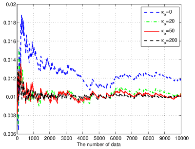
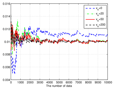
Figure 1: We assume that $\hat{F}_{s}(\cdot)$ is a normal distribution and is estimated by data $\{X_{t}\}_{t=s-W}^{s-1},\ W+1\leq s\leq T$. We consider four kinds values of $\kappa_{\alpha}=0,\ 20,\ 50,\ 200$ with $\alpha=0.01,\ W=200,\ T=10200$. Note that, $\hat{\alpha}(W)=\alpha$, we simulate the data $\{X_{s}\}_{s=1}^{T}$ two times, and plot the value of $\hat{\alpha}(s+W),\ 1\leq s\leq 10000$ in the left and right pictures.

We first determine the value of $\kappa_{\alpha}$. By equation (2.7) in Remark 2.2, we obtain that $\kappa_{\alpha}<2L(T-W)<400$. In Figure 1, we use the normal distribution $\hat{F}_{s}(\cdot)$ to approximate $N(0,0.01)$ and $\kappa_{\alpha}\left[\hat{\alpha}(\bm{X}_{s-1})-\alpha\right]$ to adjust VaR $\text{VaR}_{\alpha}(\hat{F}_{s}(\cdot))$ of $X_{s}$, when $\kappa_{\alpha}=0$, $\hat{\alpha}(\bm{X}_{s})$ is the violation rate of $\{X_{t}\}_{t=s-W}^{s-1},\ W+1\leq s\leq T$ under distribution $\hat{F}_{s}(\cdot)$ and the performance of $\text{VaR}_{\alpha}(\hat{F}_{s}(\cdot))$ is poor. On the contrary, we can see that the adjustment VaR

$$\text{VaR}^{\text{adj}}_{\alpha}(\hat{F}_{s}(\cdot))=\text{VaR}_{\alpha}(\hat{F}_{s}(\cdot))+\kappa_{\alpha}\left[\hat{\alpha}(\bm{X}_{s-1})-\alpha\right]$$

performs better with the large value $\kappa_{\alpha}$, which coincides with the results of Theorem 2.1.

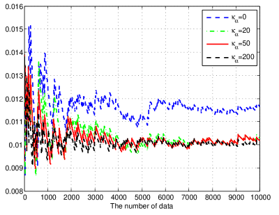
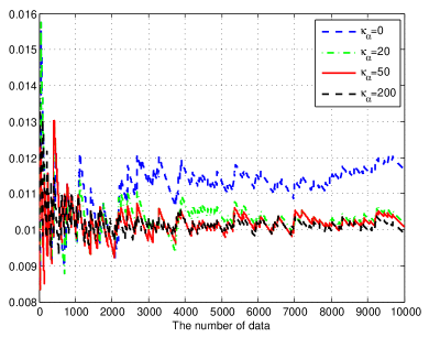
Figure 2: We assume that $\hat{F}_{t}(\cdot)$ is an empirical distribution and is estimated by data $\{X_{t}\}_{t=s-W}^{s-1},\ W+1\leq s\leq T$. We consider four kinds values of $\kappa_{\alpha}=0,\ 20,\ 50,\ 200$ with $\alpha=0.01,\ W=200,\ T=10200$. Note that, $\hat{\alpha}(W)=\alpha$, we simulate the data $\{X_{s}\}_{s=1}^{T}$ two times, and plot the value of $\hat{\alpha}(s+W),\ 1\leq s\leq 10000$ in pictures 1 and 2.

In Figure 2, we use the empirical distribution $\hat{F}_{s}(\cdot)$ to approximate $N(0,0.01)$, and $\kappa_{\alpha}\left[\hat{\alpha}(\bm{X}_{s-1})-\alpha\right]$ to adjust VaR $\text{VaR}_{\alpha}(\hat{F}_{s}(\cdot))$ of $X_{s}$. Similar to the performance of the adjusted VaR in Figure 1, the left and right pictures of Figure 2 indicate that the adjustment VaR performs better with a large value $\kappa_{\alpha}$, which verifies the results of Theorem 2.1.

Remark 3.1.

Figure 1 and Figure 2 indicate that we can use the adjusted term $\kappa_{\alpha}\left[\hat{\alpha}(\bm{X}_{s-1})-\alpha\right]$ to adjust different distributions estimation, that is, the normal distribution and empirical distribution, such that the adjusted VaR $\text{VaR}^{\text{adj}}_{\alpha}(\hat{F}_{s}(\cdot))$ has better performance. Furthermore, we can show that the performance of $\text{VaR}^{\text{adj}}_{\alpha}(\hat{F}_{s}(\cdot))$ does not depend on the length of historical data $W$.

3.2 Empirical Analysis

Next, we consider the S&P500 stock Index. We denote the log-returns daily data of S&P500 Index as the sequence $\{X_{s}\}_{s=1}^{T}$, which is taken from Mar. 22, 2017 to Dec. 31, 2019, with a total of $n=700$ daily data values.

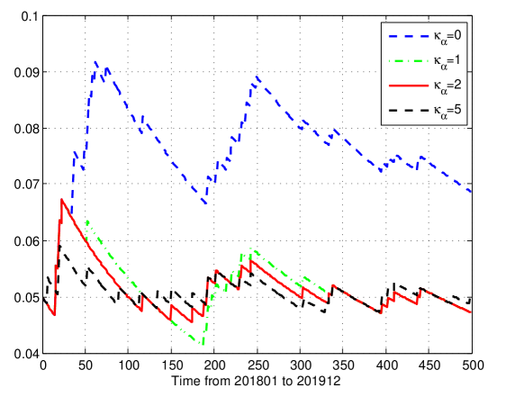
Figure 3: We assume that $\hat{F}_{s}(\cdot)$ is a normal distribution and is estimated by data $\{X_{t}\}_{t=s-W}^{s-1},\ W+1\leq s\leq T$. We consider four kinds values of $\kappa_{\alpha}=0,\ 1,\ 2,\ 5$ with $\alpha=0.05,\ W=200,\ T=700$. $\hat{\alpha}(W)=\alpha$, and we plot the value of $\hat{\alpha}(s+W),\ 1\leq s\leq 500$.

By equation (2.7) in Remark 2.2, we obtain that $\kappa_{\alpha}<2L(T-W)<20$. In Figure 3, we use the normal distribution $\hat{F}_{s}(\cdot)$ to approximate the true distribution of log return of the S&P500 Index at time $s$. We can see that the adjusted VaR $\text{VaR}^{\text{adj}}_{\alpha}(\hat{F}_{s}(\cdot))$ performs better with the largest value $\kappa_{\alpha}=5$, which coincides with the results of Theorem 2.1. The value of $\hat{\alpha}(\bm{X}_{s})$ is stable and nearly at the risk level $\alpha=0.05$. Details regarding the testing of $\text{VaR}^{\text{adj}}_{\alpha}(\hat{F}_{s}(\cdot))$ are presented in Table 1.

Table 1: Test results of S&P500 Index with $\alpha=0.05$

Model	Time	$\kappa_{\alpha}$	$\hat{\alpha}(\bm{X}_{T})$	$\text{LR}^{T}_{\text{uc}}$	$\text{LR}^{T}_{\text{ind}}$	$100\overline{\text{VaR}}$
$\text{VaR}^{\text{adj}}_{\alpha}(\hat{F}_{T}(\cdot))$:	201801-201912	0	0.0687	0.0125	0.0012	1.43
	201801-201912	1	0.0472	0.6850	0.0994	1.62
	201801-201912	2	0.0472	0.6850	0.0994	1.72
	201801-201912	5	0.0501	0.9918	0.5157	1.84

In Table 1, we show $\hat{\alpha}(\bm{X}_{T})$ at end time $T$, the $p$-value test $\text{LR}^{T}_{\text{uc}}$, the independent test of violations point $\text{LR}^{T}_{\text{ind}}$, and 100 time average values of adjusted VaR $100\overline{\text{VaR}}$ under four kinds of values of $\kappa_{\alpha}=0,\ 1,\ 2,\ 5$. When $\kappa_{\alpha}=5$, we can see that the values of testing $\text{LR}^{T}_{\text{uc}}$ and $\text{LR}^{T}_{\text{ind}}$ are nearly $1$, which indicates that the model (2.2) can significantly improve the performance of VaR under the distribution estimation $\hat{F}(\cdot)$. However, the value of $100\overline{\text{VaR}}$ increases with $\kappa_{\alpha}$.

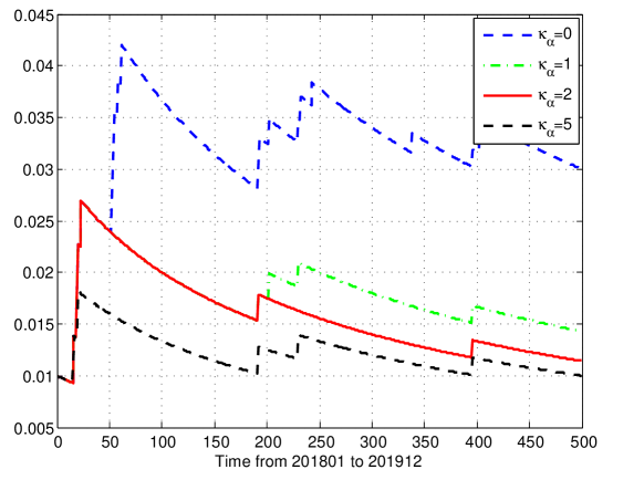
Figure 4: We assume that $\hat{F}_{s}(\cdot)$ is a normal distribution and is estimated by data $\{X_{t}\}_{t=s-W}^{s-1},\ W+1\leq s\leq T$. We consider four kinds of values of $\kappa_{\alpha}=0,\ 1,\ 2,\ 5$ with $\alpha=0.01,\ W=200,\ T=700$. $\hat{\alpha}(W)=\alpha$, we plot the value of $\hat{\alpha}(s+W),\ 1\leq s\leq 500$.

Table 2: Test results of S&P500 Index with $\alpha=0.01$

Model	Time	$\kappa_{\alpha}$	$\hat{\alpha}(\bm{X}_{T})$	$\text{LR}^{T}_{\text{uc}}$	$\text{LR}^{T}_{\text{ind}}$	$100\overline{\text{VaR}}$
$\text{VaR}^{\text{adj}}_{\alpha}(\hat{F}_{T}(\cdot))$:	201801-201912	0	0.0300	0.0000	0.0324	2.04
	201801-201912	1	0.0143	0.2131	0.1094	2.83
	201801-201912	2	0.0114	0.6596	0.0542	3.20
	201801-201912	5	0.0100	0.9964	1.0000	3.12

In Table 2, we show $\hat{\alpha}(\bm{X}_{T})$ at end time $T$, the $p$-value test $\text{LR}^{T}_{\text{uc}}$, the independent test of violations point $\text{LR}^{T}_{\text{ind}}$, and 100 time average value of adjustment VaR $100\overline{\text{VaR}}$ under four kinds of values of $\kappa_{\alpha}=0,\ 1,\ 2,\ 5$. When $\kappa_{\alpha}=5$, we can see that the values of testing $\text{LR}^{T}_{\text{uc}}$ is improved to $0.9964$ comparing to $\kappa_{\alpha}=0,\ 1,\ 2$, which indicates that the model (2.2) can significantly improve the performance of VaR under the distribution estimation $\hat{F}(\cdot)$ with different risk levels $\alpha$.

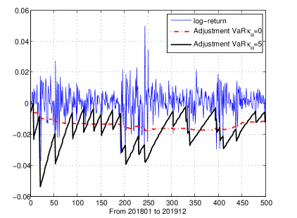
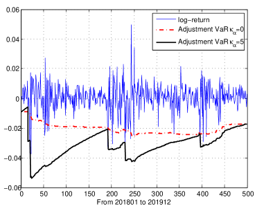
Figure 5: We assume that $\hat{F}_{s}(\cdot)$ is a normal distribution and is estimated by data $\{X_{t}\}_{t=s-W}^{s-1},\ W+1\leq s\leq T$. Let $\kappa_{\alpha}=0,5$, $\alpha=0.05,0.01,\ W=200,\ T=700$. $\hat{\alpha}(W)=\alpha$, and we plot the value of adjusted VaR $\text{VaR}^{\text{adj}}_{\alpha}(\hat{F}_{s}(\cdot))$ and the log return of S&P500, $1\leq s\leq 500$. The left picture is with $\alpha=0.05$, and the right picture is with $\alpha=0.01$.

In Figure 5, the left picture indicates that the adjusted VaR with $\kappa_{\alpha}=5$ can capture the local changes of the log return of S&P500 for $\alpha=0.05$ compared with VaR under the normal distribution with $\kappa_{\alpha}=0$. A similar process can be seen in the right image with $\alpha=0.01$.

In this section, we show the performances of the adjusted VaR $\text{VaR}^{\text{adj}}_{\alpha}(\hat{F}_{s}(\cdot))$ with risk value $\alpha=0.05,\ 0.01$ and $\kappa_{\alpha}=0,1,2,5$ under normal distribution estimation $\hat{F}_{s}(\cdot)$. We can see that $\text{VaR}^{\text{adj}}_{\alpha}(\hat{F}_{s}(\cdot))$ can improve the performances of VaR under distribution $\hat{F}_{s}(\cdot)$ at least for the log return of the Index S&P500. Furthermore, we also use the NASDAQ Index and the CSI300 Index to check the adjusted VaR $\text{VaR}^{\text{adj}}_{\alpha}(\hat{F}_{s}(\cdot))$ under the normal and empirical distributions with different values of $W$. In general, we find that $\text{VaR}^{\text{adj}}_{\alpha}(\hat{F}_{s}(\cdot))$ can obtain excellent performance with an adaptive $\kappa_{\alpha}$.

4 Conclusion

This study developed a compensatory model to improve the quantile estimation of time series $\{X_{n}\}_{n=1}^{\infty}$ under given distribution estimation $\{\hat{F}_{n}(\cdot)\}_{n=1}^{\infty}$. Traditional statistical methods include estimating the distribution behind the time series. By introducing a penalty term in the definition of the counting function, this study employs the method of adjusting the quantile of distribution estimation $\hat{F}_{n}(\cdot)$. There is a control ability factor $\kappa_{\alpha}$ in the penalty term, that is used to control the distance between the cumulative sum of the counting function and quantile level $\alpha$. Thus, the penalty term can adjust and improve the performance of the quantile of $\hat{F}_{n}(\cdot)$. Through simulation and empirical analysis, we showed that the compensatory model can significantly improve the performance of VaR under a given distribution. In particular, the compensatory model is not dependent on the value of quantile level $\alpha$ and the length of historical data $W$.

We would like to note that the method developed in this study is not used to estimate the true distribution behind the time series, but to improve the performance of a general distribution estimation. Using the compensatory model presented in this study, we have calculated the adjustment $\alpha$ quantile for the S&P500 Index, the NASDAQ Index, and the CSI300 Index under quantile level $\alpha=0.05,0.01$, which verifies the usefulness of the compensatory model. Therefore, this compensatory model could be used to conduct data analysis for stock markets, bond markets, and cryptocurrency markets.

References

- Abad et al. (2014) P. Abad, S. Benito, and C. López. A comprehensive review of Value at Risk methodologies. The Spanish Review of Financial Economics, 12:1:15–32, 2014.
- Alexander and Dakos (2020) C. Alexander and M. Dakos. A critical investigation of cryptocurrency data and analysis. Quantitative Finance, 20(2):173–188, 2020.
- Ardia et al. (2019) D. Ardia, K. Bluteau, and M. Rüede. Regime changes in Bitcoin GARCH volatility dynamics. Finance Research Letters, 29:266–271, 2019.
- Avellaneda et al. (1995) M. Avellaneda, A. Levy, and A. Parás. Pricing and hedging derivative securities in markets with uncertain volatilities. Applied Mathematical Finance, 2:73–88, 1995.
- Bollerslev (1986) T. Bollerslev. Generalized autoregressive conditional heteroskedasticity. Journal of Econometrics, 31:307–327, 1986.
- Chen et al. (2019) Y. Chen, Z. Wang, and Z. Zhang. Mark to market value at risk. Journal of Econometrics, 208:1:299–321, 2019.
- Chen and Epstein (2002) Z. Chen and L. Epstein. Ambiguity, risk, and asset returns in continuous time. Econometrica, 70(4):1403–1443, 2002.
- Cont (2006) R. Cont. Model uncertainty and its impact on the pricing of derivative instruments. Mathematical Finance, 16:519–547, 2006.
- De Rossi and Harvey (2006) G. De Rossi and A.C. Harvey. Time-varying quantiles. Faculty of Economics, Cambridge:CWPE 0649, 2006.
- De Rossi and Harvey (2009) G. De Rossi and A.C. Harvey. Quantiles, expectiles and splines. Journal of Econometrics, 152:179–185, 2009.
- Dekkers and De Hana (1989) A. L. M. Dekkers and L. De Hana. On the estimation of the extreme-value index and large quantile estimation. The Annals of Statistics, 17(4):1795–1832, 1989.
- Duffie and Pan (1997) D. Duffie and J. Pan. An overview of value at risk. Journal of Derivatives, 4:7–49, 1997.
- Engle (1982) Robert F. Engle. Autoregressive Conditional Heteroskedasticity with Estimates of the Variance of United Kingdom Inflation. Econometrica, 50(4):987–1007, 1982.
- Engle and Manganelli (2004) Robert F. Engle and S. Manganelli. CAViaR: Conditional autoregressive value at risk by regression quantiles. Journal of Business & Economic Statistics, 22:4:367–381, 2004.
- Epstein and Ji (2013) L. G. Epstein and S. Ji. Ambiguous volatility and asset pricing in continuous time. Review of Financial Studies, 26(7):1740–1786, 2013.
- Francisco and Fuller (1991) C. A. Francisco and W. A. Fuller. Quantile estimation with a complex survey design. The Annals of Statistics, 19(1):454–469, 1991.
- Heidelberger and Lewis (1984) P. Heidelberger and P. A. W. Lewis. Quantile estimation in dependent sequences. Operations Research, 32(1):185–209, 1984.
- Hosking and Wallis (1987) J. R.M. Hosking and J. R. Wallis. Parameter and quantile estimation for the generalized pareto distribution. Technometrics, 29(3):339–349, 1987.
- Huber (1981) P. J. Huber. Robust Statistics. Wiley Series in Probability and Mathematical Statistics. John Wiley & Sons, Inc., New York, 3rd edition, 1981.
- Jorion (2010) Ph. Jorion. Risk management. Annual Review of Financial Economics, 2(1):347–365, 2010.
- Kerkhof et al. (2010) J. Kerkhof, B. Melenberg, and H. Schumacher. Model risk and capital reserves. Journal of Banking & Finance, 34:267–279, 2010.
- Koenker and Zhao (1996) R. Koenker and Q. Zhao. Conditional quantile estimation and inference for Arch models. Econometric Theory, 12(5):793–813, 1996.
- Kuester et al. (2006) K. Kuester, S. Mittnik, and M. S. Paolella. Value-at-Risk Prediction: A comparison of alternative strategies. Journal of Financial Econometrics, 4(1):53–89, 2006.
- Maciel (2020) L. Maciel. Cryptocurrencies value-at-risk and expected shortfall: Do regimeswitching volatility models improve forecasting. International Journal of Finance & Economics, pages 1–16, 2020.
- Mease et al. (2007) D. Mease, A. J. Wyner, and A. Buja. Boosted classification trees and class probability quantile estimation. Journal of Machine Learning Research, 8(16):409–439, 2007.
- Peng (1997) S. Peng. Backward SDE and related g-expectation. Backward stochastic differential equations (Paris, 1995-1996) 141-159. Pitman Res. Notes Math. Ser., Longman, Harlow, 1997.
- Peng (2004) S. Peng. Filtration consistent nonlinear expectations and evaluations of contingent claims. Acta Mathematicae Applicatae Sinica, 20:1–24, 2004.
- Peng (2005) S. Peng. Nonlinear expectations and nonlinear Markov chains. Acta Mathematicae Applicatae Sinica, 26B:159–184, 2005.
- Peng (2019) S. Peng. Nonlinear Expectations and Stochastic Calculus under Uncertainty, pages 1–212. Springer, Berlin, Heidelberg, 2019.
- Peng and Yang (2021) S. Peng and S. Yang. Distributional uncertainty of the financial time series measured by g-expectation. Theory of Probability and Its Applications, 66(4):914–928, 2021.
- Peng et al. (2020) S. Peng, S. Yang, and J. Yao. Improving value-at-risk prediction under model uncertainty. Journal of Financial Econometrics, doi:10.1093/jjfinec/nbaa022:1–30, 2020.
- Takeuchi et al. (2006) I. Takeuchi, Q. V. Le, T. D. Sears, and A. J. Smola. Nonparametric quantile estimation. Journal of Machine Learning Research, 7(45):1231–1264, 2006.
- Trucíos (2019) C. Trucíos. Forecasting Bitcoin risk measures: A robust approach. International Journal of Forecasting, 35(3):836–847, 2019.
- Trucíos and Taylor (2020) C. Trucíos and James W. Taylor. Forecasting Value-at-Risk and Expected Shortfall of Cryptocurrencies using Combinations based on Jump-Robust and Regime-Switching Models. DOI: 10.13140/RG.2.2.27175.98728:1–23, 2020.
- Walley (1991) P. Walley. Statistical reasoning with imprecise probabilities. Monographs on Statistics and Applied Probability, 42. Chapman and Hall, Ltd., London, 1991.
- Wang et al. (2020) G. Wang, K. Zhou, G. Li, and W. K. Li. Hybrid quantile estimation for asymmetric power GARCH models. Journal of Econometrics, https://doi.org/10.1016/j.jeconom.2020.05.005:1–22, 2020.
- Yiu et al. (2010) K. Yiu, J. Liu, T. Siu, and W Ching. Optimal portfolios with regime switching and value-at-risk constraint. Automatica, 46:979–989, 2010.
- Zhang and Nadarajah (2017) Y. Zhang and S. Nadarajah. A review of backtesting for value at risk. Communications in Statistics - Theory and Methods, pages 1–24, 2017.
- Zhu et al. (2016) D. Zhu, Y. Xie, W. Ching, and T Siu. Optimal portfolios with maximum value-at-risk constraint under a hidden markovian regime-switching model. Automatica, 74:194–205, 2016.