Analyzing population dynamics models via Sumudu transform

Abstract.

This study demonstrates how to construct the solutions of a more general form of population dynamics models via a blend of variational iterative method with Sumudu transform. In this paper, population growth models are formulated in the form of delay differential equations of pantograph type which is a general form for the existing models. Innovative ways are presented for obtaining the solutions of population growth models where other analytic methods fail. Stimulating procedures for finding patterns and regularities in seemingly chaotic processes have been elucidated in this paper. How, when and why the changes in population sizes occur can be deduced through this study.

1. Introduction

There is a growing need to understand the dynamics that affect populations of organisms over time. The study of population dynamics can help to understand what influences the abundance of organisms at a particular time. It can also help to find answer to why the abundance of a species of organisms changes over time. Finding patterns and regularities in seemingly chaotic processes is through the studies on population dynamics. Prediction on certain species of animals or plants which are under the danger of extinction is as a result of studies on population dynamics. How a deadly virus spreads can only be understood and explained through population dynamics. There are several reports on using mathematical models to analyze the population dynamics [1, 2, 3, 4, 5, 6]. Mathematical modeling of physical situations involves differential equations. Differential equations are indispensable for the description of many real-world phenomena. Differential equations are generally known as powerful tools for the study, analysis and prediction of essential real-world occurrences.

Let $x(t)$ denote the population size at time $t$ and let $r$ be the population growth rate (birth rate minus death rate). In 1798, the studies of Malthus on population growth was summarized by the model [7],

(1.1) $$x^{\prime}(t)=rx(t),\ \ x(0)=x_{0}.$$

Malthus was a British demographer and and came up with the model which is given by (1.1). The model was as a result of studies of demographic data which were more than a hundred years. Solving the initial value problem (1.1) by separating the variables yields

(1.2) $$x(t)=x_{0}e^{rt}.$$

Obviously, it is an exponential model. It speculates exponential growth if $r>0$ and represents the traditional decay if $r<0.$ Such a model may be valid for only a short period or only when the population is scarce and resources are abundant. It is a common knowledge that at a certain level of growth of a population, certain negative factors do set in which hinder further growth. Instances of such negative factors include poor agricultural yields which could cause starvation due to food shortages, air pollution as well as emergence of virus and diseases that could affect the lifespans of the organisms. Indeed, prediction of the model by Malthus is unrealistic in nature. In 1838, Verhulst considered the fact that resources are limited and proposed the logistic growth model [8],

(1.3) $$x^{\prime}(t)=rx(t)\left(1-\frac{x(t)}{K}\right),$$

where $r(>0)$ is the intrinsic growth rate and $K(>0)$ is the carrying capacity of the population. Given an initial condition $x_{0},$ the solution for the logistic growth model is obtained as

(1.4) $$x(t)=\frac{x_{0}K}{x_{0}+(K-x_{0})e^{-rt}}.$$

Competition occurs as $x(t)$ gets large and $x(t)$ approaches $K$ as $t\rightarrow\infty.$ The logistic growth model predicts a rapid growth when $x(t)$ is smaller than $K$ and it stipulates decrease of growth when $x(t)$ approaches $K.$ If $x_{0}=K,$ the population remains in time at $x(t)=K,$ which is an equilibrium point. Naturally, occurrences of processes are not instantaneous. Behavioral responses of organisms to environmental changes takes a unit of time before it is feasible. Recovery of grasses after grazing takes a unit of time. Ordinary differential equations are not enough to model these kinds of scenarios. The growth rate $x^{\prime}(t)$ at time $t$ depends on both $x(t)$ and $x(t-\tau),$ where $x(t-\tau)$ is the population size in some period in the past $(t-\tau)$ and $\tau>0$ is a constant. In 1948, Hutchinson proposed a more logistic growth model that involves delay [9],

(1.5) $$x^{\prime}(t)=rx(t)\left(1-\frac{x(t-\tau)}{K}\right),\ \ x(0)=x_{0}.$$

However, the analytic solutions to equations of the form (1.5) are not possible in general. Numerical approximations have been applied to gain an insight into the behavior of such models. Research efforts over the years have been on the construction of solutions, reformulations, improvements and applications of (1.5) [5, 6, 10, 11, 12]. Recently, the research focus has been on delay differential equations with multi-proportional delays. Generally, they are being referred to as delay differential equations of pantograph type [13, 14, 15, 16]. Delay differential equations of pantograph type have received much attention because many models with proportional delays produce significant results. The results which they produce are found to be accurate and stable. Also, they are suitable for studying several models which include the case where the delay is a fraction of the time unit. Consequently, several existing models and various classes of differential equations are being reformulated and reconstructed in terms of delay differential equations of pantograph type.

The studies on population dynamics are of crucial importance as all of the processes on the earth, directly or indirectly affect the human life. The goal of this study is to present suitable reformulation and reconstruction for some existing population growth models in terms of delay differential equations of pantograph type. An innovative method is displayed for constructing the solutions of the models where other analytic methods fail. This study shows how to find patterns and regularities in seemingly chaotic processes. Some single and interacting species population models are illustrated graphically and analyzed.

2. Description of the method

The method is presented in this section to make this study a complete paper. The account of the method which is being presented has been discussed in [17, 18, 19].

2.1. Variational iterative method

Due to its flexibility, consistency and effectiveness, variational iterative method is more preferred when compared to other well-known methods (See e.g, [20, 21] and references there in). The elevation which is a blend of variational iterative method with Laplace transform (See e.g, [20, 21]) and Sumudu transform (See e.g, [18]) has also been considered. The Sumudu transform can be described as a mutation of Laplace transform. Sumudu transform has been proved to be a simple, effective and universal way for obtaining Lagrange multiplier. For a given property of Laplace transform, a corresponding property can be obtained for Sumudu transform and vice versa (See e.g, [22, 23, 24]). Sumudu transform can be applied to a given function $f(t)$ which satisfies the Dirichlet conditions:

• it is single valued function which may have a finite number of isolated discontinues for $t>0.$

• it remains less than $be^{-a_{0}t}$ as $t$ approaches $\infty,$ where $b$ is a positive constant and $a_{0}$ is a real positive number.

Sumudu transform has been employed to obtain the solutions of differential equations which are of several forms [25, 26, 27, 28].

2.2. Presentation of Sumudu transform

The concept was proposed by Watugala [22]. It is an integral transform and it is suitable for solving several problems which are modeled by differential equations. Let $F(u)$ denote the Sumudu transform of a function $f(t).$ For all real numbers $t\geq 0,$

(2.1) $$F(u)=S\left[f(t)\right]=\int^{\infty}_{0}f(ut)e^{-t}dt.$$

The Sumudu transform for the integer order derivatives is expressed as

(2.2) $$S\left[\frac{df(t)}{dt}\right]=\frac{1}{u}\left[F(u)-f(0)\right].$$

For the $n$-order derivative, the Sumudu transform is given as

(2.3) $$S\left[\frac{d^{n}f(t)}{dt^{n}}\right]=\frac{1}{u^{n}}\left[F(u)-\displaystyle\sum_{k=0}^{n-1}u^{k}\frac{d^{k}f(t)}{dt^{k}}|_{x=0}\right].$$

Linearity of Sumudu transform can be easily established and Sumudu transform is also credited for preserving units and linear functions (See e.g, [22, 23]). These essential properties make solving problems easy by using Sumudu transform without the need to resort to a new frequency domain. The focal points of the Sumudu transform are exhibited for a broad nonlinear problem

(2.4) $$\frac{d^{n}x(t)}{dt^{n}}+R\left[x(t)\right]+N\left[x(t)\right]=g(t),$$

subject to the initial conditions

(2.5) $$x^{(k)}(0)=a_{k},$$

where $x^{(k)}(0)=\frac{d^{k}x(0)}{dt^{k}},$ $k=0,1,...,n-1,$ $R$ is a linear operator, $N$ is a nonlinear operator, $g(t)$ is a given continuous function and the highest order derivative is $\frac{d^{n}x(t)}{dt^{n}}.$

Let $X(u)=S[x(t)],$ by taking the Sumudu transform of (2.4), its linear part is transformed into an algebraic equation of the form

(2.6) $$\frac{1}{u^{n}}X(u)-\displaystyle\sum_{k=0}^{n-1}\frac{1}{u^{n-k}}y^{(k)}(0)=S\left[g(t)-R\left[x\right]-N\left[x\right]\right].$$

The sequence of iteration is deduced as

(2.7) $$X_{n+1}(u)=X_{n}(u)+{\varphi}(u)\left(\frac{1}{u^{n}}X_{n}(u)-\displaystyle\sum_{k=0}^{n-1}\frac{1}{u^{n-k}}x^{(k)}(0)-S\left[g(t)-R\left[x\right]-N\left[x\right]\right]\right),$$

where ${\varphi}(u)$ is the Lagrange multiplier. The classical variation operator is taken on both sides of (2.7) while $S\left[R\left[x\right]+N\left[x\right]\right]$ is considered as restricted term. This gives

(2.8) $$\delta X_{n+1}(u)=\delta X_{n}(u)+{\varphi}(u)\frac{1}{u^{n}}\delta X_{n}(u),$$

from which it is obtained that

(2.9) $${\varphi}(u)=-u^{n}.$$

Substitute (2.9) into (2.7) and take the inverse-Sumudu transform $S^{-1}$ of (2.7) to obtain

(2.10) $$x_{n+1}(t) = x_{n}(t)+S^{-1}\left[-u^{n}\left(\frac{1}{u^{n}}X(u)-\displaystyle\sum_{k=0}^{n-1}\frac{1}{u^{n-k}}x^{(k)}(0)-S\left[g(t)-R\left[x\right]-N\left[x\right]\right]\right)\right],$$

$$= x_{1}(t)+S^{-1}\left[u^{n}\left(S\left[g(t)-R\left[x(t)\right]-N\left[x(t)\right]\right]\right)\right],$$

where

(2.11) $$x_{1}(x) = S^{-1}\left[\displaystyle\sum_{k=0}^{n-1}u^{k}x^{(k)}(0)\right]$$

$$= x(0)+x^{\prime}(0)t+...+\frac{x^{n-1}(0)t^{n-1}}{(n-1)!}.$$

2.3. Variable coefficient nonlinear equation

Suppose the broad nonlinear problem (2.4) contains variable coefficients which makes it to become

(2.12) $$\frac{d^{n}x(t)}{dt^{n}}+\alpha R_{1}[x(t)]+\beta(t)R_{2}[x(t)]+N\left[x(t)\right]=g(t),$$

where $\alpha$ is a constant and $\beta(t)$ is a variable coefficient, $R_{1}$ and $R_{2}$ are linear operators and other terms remain as defined in (2.4). The Sumudu transform of (2.12) is taken to get

(2.13) $$X_{n+1}(u) = X_{n}(u)+{\varphi}(u)(\frac{1}{u^{n}}X_{n}(u)-\displaystyle\sum_{k=0}^{n-1}\frac{1}{u^{n-k}}x^{(k)}(0)$$

$$-S\left[g(t)-\alpha R_{1}[x]-\beta(t)R_{2}[x]-N\left[x\right]\right]).$$

Here, the restricted term is $S\left[\beta(t)R_{2}[x]+N\left[x\right]\right].$ Obtain the Lagrange multiplier ${\varphi}(u).$ The rest of computation processes are the same with the presentations in Section 2.2.

3. Main Results

3.1. Modified Hutchinson’s model

We consider the reconstruction of the model of Hutchinson (1948) in terms of delay differential equations of pantograph type to gain insight into situation which include the case where the delay is a fraction of the time unit. A suitable reformulation is presented to the Hutchinson’s model (1.5).

Consider

(3.1) $$x^{\prime}(t) = rx(t)\left(1-\frac{x(\alpha t)}{K}\right),~{}t>0,$$

$$x(0) = x_{0},$$

where $r$ and $K$ have the same meaning as in the previous equations and $\alpha\in[0,1].$

Here, three case will be considered for the values of $\alpha$ which are $0,1$ and $(0,1).$

Case one: $\alpha=0.$

For $\alpha=0,$ equation (3.1) becomes

(3.2) $$x^{\prime}(t) = rx(t)\left(1-\frac{x_{0}}{K}\right),\ \ x(0)=x_{0}.$$

Equation (3.2) is a modified form that involves the carrying capacity of the population for the model of Malthus (1798). The solution of (3.2) is given by

(3.3) $$x(t)=x_{0}e^{r\left(1-\frac{x_{0}}{K}\right)t},$$

which is a modified exponential growth model. Figure 1 displays the solution for modified Hutchinson’s model when $\alpha=0.$

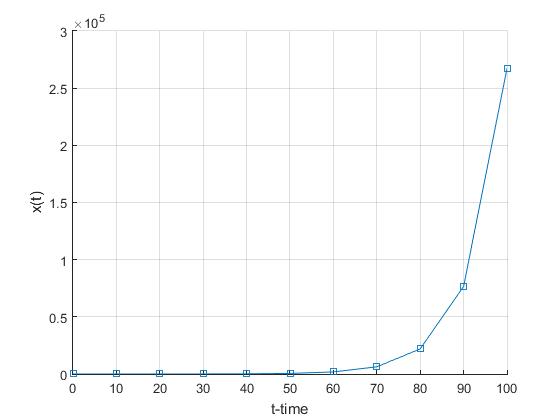
Figure 1. Graph of $x(t)$ for $x_{0}=1,K=3000$ & $r=0.125$.

Case Two: $\alpha=1.$

Taking $\alpha=1$ in (3.1) gives the logistic growth model (1.3) and its solution is given by (1.4). Figure 2 displays the solution for the logistic growth model where $x(t),$ which is the population size converges to $K,$ which is the carrying capacity of the population.

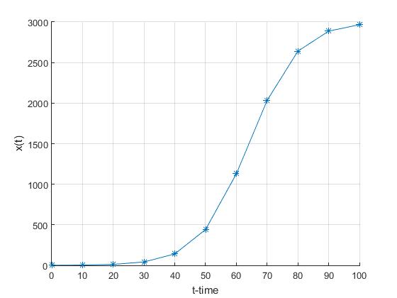
Figure 2. Graph of $x(t)$ for $x_{0}=1,K=3000$ & $r=0.125$.

Case Three: $\alpha\in(0,1).$

The solution is constructed by using a blend of VIM with ST. Taking the ST of (3.1) gives

(3.4) $$\frac{X(u)}{u}-\frac{x(0)}{u}=S\left[rx(t)\left(1-\frac{x(\alpha t)}{K}\right)\right].$$

Since $x(0)=x_{0},$ equation (3.4) becomes

(3.5) $$\frac{X(u)}{u}-\frac{x_{0}}{u}=S\left[rx(t)\left(1-\frac{x(\alpha t)}{K}\right)\right].$$

Thus for $n\in\mathbb{N},$ the variational iteration formula is given by

(3.6) $$X_{n+1}(u) = X_{n}(u)+{\varphi}(u)\left(\frac{X_{n}(u)}{u}-\frac{x_{0}}{u}-S\left[rx_{n}(t)\left(1-\frac{x_{n}(\alpha t)}{K}\right)\right]\right).$$

The classical variation operator on both sides of (3.6) is taken and the term $rx_{n}(t)\left(1-\frac{x_{n}(\alpha t)}{K}\right)$ is considered as the restricted variation. The Lagrange multiplier is then obtained as

(3.7) $${\varphi}(u)=-u.$$

The inverse-Sumudu transform, $S^{-1}$ of (3.6) is taken which gives the explicit iteration formula

(3.8) $$x_{n+1}(t) = x_{n}(t)+S^{-1}\left[-u\left(\frac{X_{n}(u)}{u}-\frac{x_{0}}{u}-S\left[rx_{n}(t)\left(1-\frac{x_{n}(\alpha t)}{K}\right)\right]\right)\right]$$

$$= x_{0}+S^{-1}\left[ru\left(S\left[x_{n}(t)\right]-\frac{1}{K}S\left[x_{n}(t)x_{n}(\alpha t)\right]\right)\right],$$

where the initial approximation is given by $x_{1}(t)=x(0)=x_{0}.$ Recall the decomposition of a nonlinear term ${}^{\prime}N(x)^{\prime}$ as

$$N(x)=\displaystyle\sum_{i=0}^{\infty}A_{i}=\frac{1}{i!}\left[\frac{d^{i}}{d{\theta}^{i}}f\left(\displaystyle\sum_{n=0}^{\infty}{\theta}^{n}v_{n}\right)\right]\bigg{|}_{\theta=0},$$

where $A_{i}$ is the Adomian polynomial [29]. Let $x_{n}=\displaystyle\sum_{i=0}^{n}v_{i},$ the Adomian series of the nonlinear term ${}^{\prime}x_{n}(t)x_{n}(\alpha t)^{\prime}$ reads

(3.9) $$\begin{cases}A_{0}=v_{0}^{2},\\ A_{1}=2v_{0}v_{1},\\ A_{2}=2v_{0}v_{2}+v_{1}^{2}\\ A_{3}=2v_{0}v_{3}+2v_{1}v_{2}\\ \vdots\end{cases}$$

Therefore, this yields the successive formula

(3.10) $$\begin{cases}v_{0}(t)=v(0)=x_{0},\\ v_{n+1}(t)=S^{-1}\left[ru\left(S\left[v_{n}\right]-\frac{1}{K}S\left[A_{n}\right]\right)\right],\end{cases}$$

which produces the iteration

(3.11) $$\begin{cases}v_{0}=x_{0},\\ v_{1}=x_{0}\left(1-\frac{x_{0}}{K}\right)rt,\\ v_{2}=\left[x_{0}\left(1-\frac{x_{0}}{K}\right)^{2}-\frac{x_{0}^{2}}{K}\left(1-\frac{x_{0}}{K}\right)\right]\frac{r^{2}t^{2}}{2!},\\ \\ v_{3}=\bigg{[}x_{0}\left(1-\frac{x_{0}}{K}\right)^{3}-\frac{4x_{0}^{2}}{K}\left(1-\frac{x_{0}}{K}\right)^{2}+\frac{x_{0}^{3}}{K}\left(1-\frac{x_{0}}{K}\right)\bigg{]}\frac{r^{3}t^{3}}{3!},\\ \vdots\end{cases}$$

The solution is therefore given by

(3.12) $$\begin{split}x(t)&=\displaystyle\lim_{n\rightarrow\infty}x_{n}=\displaystyle\lim_{n\rightarrow\infty}\displaystyle\sum_{i=0}^{n}v_{i}\\ &=x_{0}+x_{0}\left(1-\frac{x_{0}}{K}\right)rt+\left[x_{0}\left(1-\frac{x_{0}}{K}\right)^{2}-\frac{x_{0}^{2}}{K}\left(1-\frac{x_{0}}{K}\right)\right]\frac{r^{2}t^{2}}{2!}\\ &+\bigg{[}x_{0}\left(1-\frac{x_{0}}{K}\right)^{3}-\frac{4x_{0}^{2}}{K}\left(1-\frac{x_{0}}{K}\right)^{2}+\frac{x_{0}^{3}}{K}\left(1-\frac{x_{0}}{K}\right)\bigg{]}\frac{r^{3}t^{3}}{3!}+...\\ &=x_{0}\left(1+\left(1-\frac{x_{0}}{K}\right)rt+\frac{r^{2}\left(1-\frac{x_{0}}{K}\right)^{2}t^{2}}{2!}+\frac{r^{3}\left(1-\frac{x_{0}}{K}\right)^{3}t^{3}}{3!}+...\right)\\ &-\frac{x_{0}^{2}}{K}\left(1-\frac{x_{0}}{K}\right)\frac{r^{2}t^{2}}{2!}-\bigg{[}\frac{4x_{0}^{2}}{K}\left(1-\frac{x_{0}}{K}\right)^{2}-\frac{x_{0}^{3}}{K}\left(1-\frac{x_{0}}{K}\right)\bigg{]}\frac{r^{3}t^{3}}{3!}-...\\ &=x_{0}e^{\left(1-\frac{x_{0}}{K}\right)rt}-\frac{x_{0}^{2}}{K}\left(1-\frac{x_{0}}{K}\right)\frac{r^{2}t^{2}}{2!}-\bigg{[}\frac{4x_{0}^{2}}{K}\left(1-\frac{x_{0}}{K}\right)^{2}-\frac{x_{0}^{3}}{K}\left(1-\frac{x_{0}}{K}\right)\bigg{]}\frac{r^{3}t^{3}}{3!}-...\end{split}$$

Figure 3 displays the solution for the modified Hutchinson s model when $\alpha\in(0,1).$

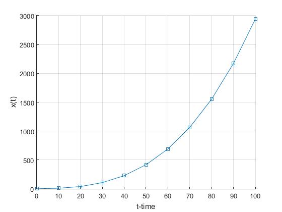
Figure 3. Graph of $x(t)$ for $x_{0}=1,K=3000$ & $r=0.125$.

3.2. Blowflies model

The blowfly model was proposed in 1954 by Nicholson (See e.g, [30]). Gurney et al. (1980) [31] introduced the delay into the model to correct the discrepancy which was noted in the Nicholson s blowflies model. The blowfly model with delay is given by

(3.13) $$x^{\prime}(t) = Px(t-\tau)e^{\left(-\frac{x(t-\tau)}{x_{0}}\right)}-\delta x(t),~{}t>0,$$

$$x(0) = x_{0},$$

where $P$ is the maximum per capita daily egg production rate, $x_{0}$ is the size at which the blowflies population reproduces at its maximum rate and $\delta$ is the per capita daily adult death rate. To gain insight into situation which include the case where the delay is a fraction of the time unit, we study a reconstruction of blowfly model in the form of delay differential equations of pantograph type.

Consider a modified blowflies model which is expressed by

(3.14) $$x^{\prime}(t) = Px(\alpha t)e^{\left(-\frac{x(\alpha t)}{x_{0}}\right)}-\delta x(t),~{}t>0,$$

$$x(0) = x_{0},$$

where definitions of $P,x_{0}$ and $\delta$ remain the same while $\alpha\in[0,1].$

Case One: $\alpha=0.$

For $\alpha=0,$ equation (3.14)

$$x^{\prime}(t)+\delta x(t)=Px_{0}e^{-1},~{}x(0)=x_{0},$$

which is a linear ordinary differential equation of degree one. Its solution is given

(3.15) $$x(t)=x_{0}\left(Pe^{-1}+\frac{1-Pe^{-1}}{e^{\delta t}}\right).$$

An obvious deduction from (3.15) is that $x(t)\rightarrow Px_{0}e^{-1}$ as $t\rightarrow\infty.$ Figure 4 displays the solution for the modified blowflies model in the form of delay differential equations of pantograph type when $\alpha=0.$

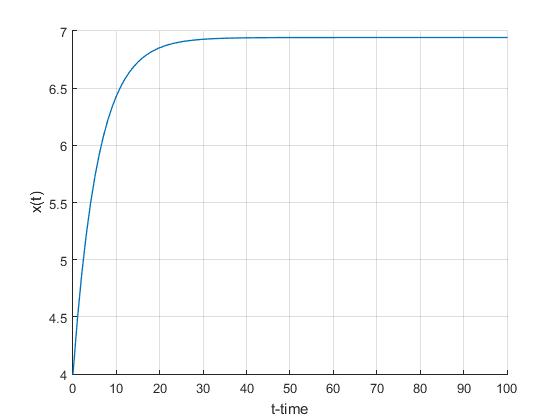
Figure 4. Graph of $x(t)$ for $x_{0}=4,P=2$ & $\delta=0.175$.

Case Two: $\alpha\in(0,1].$

When $\alpha=1,$ observe that it is not easy to obtain by analytical method, the solution of the nonlinear first order differential equation

$$x^{\prime}(t)-\left(Pe^{\left(-\frac{x(t)}{x_{0}}\right)}-\delta\right)x(t)=0,~{}x(0)=x_{0}.$$

Therefore, a blend of VIM with ST will be used to obtain the solution when $\alpha\in(0,1].$

Solution: By taking the ST of (3.14), we obtain

(3.16) $$\frac{X(u)}{u}-\frac{x(0)}{u}=PS\left[x(\alpha t)e^{\left(-\frac{x(\alpha t)}{x_{0}}\right)}\right]-\delta S\left[x(t)\right].$$

Since $x(0)=x_{0},$ equation (3.16) gives

(3.17) $$\frac{X(u)}{u}-\frac{x_{0}}{u}=PS\left[x(\alpha t)e^{\left(-\frac{x(\alpha t)}{x_{0}}\right)}\right]-\delta S\left[x(t)\right].$$

Thus for $n\in\mathbb{N},$ the variational iteration formula is given by

(3.18) $$X_{n+1}(u) = X_{n}(u)+{\varphi}(u)\left(\frac{X_{n}(u)}{u}-\frac{x_{0}}{u}-PS\left[x_{n}(\alpha t)e^{\left(-\frac{x_{n}(\alpha t)}{x_{0}}\right)}\right]+\delta S\left[x_{n}(t)\right]\right).$$

The classical variation operator on both sides of (3.18) is taken and the term $Px(\alpha t)e^{\left(-\frac{x(\alpha t)}{x_{0}}\right)}$ is considered as the restricted variation. The Lagrange multiplier is then obtained as

(3.19) $${\varphi}(u)=-u.$$

Taking the inverse-Sumudu transform, $S^{-1}$ of (3.18) gives the explicit iteration formula

(3.20) $$x_{n+1}(t) = x_{n}(t)+S^{-1}\left[-u\left(\frac{X_{n}(u)}{u}-\frac{x_{0}}{u}-PS\left[x_{n}(\alpha t)e^{\left(-\frac{x_{n}(\alpha t)}{x_{0}}\right)}\right]+\delta S\left[x_{n}(t)\right]\right)\right]$$

$$= x_{0}+S^{-1}\left[u\left(PS\left[x_{n}(\alpha t)e^{\left(-\frac{x_{n}(\alpha t)}{x_{0}}\right)}\right]-\delta S\left[x(t)\right]\right)\right],$$

where the initial approximation is given by $x_{1}(t)=x(0)=x_{0}.$ Recall the decomposition

$$N(x)=\displaystyle\sum_{i=0}^{\infty}A_{i}=\frac{1}{i!}\left[\frac{d^{i}}{d{\theta}^{i}}f\left(\displaystyle\sum_{n=0}^{\infty}{\theta}^{n}v_{n}\right)\right]\bigg{|}_{\theta=0},$$

where $N(x)$ is the nonlinear term and $A_{i}$ is the Adomian polynomial [29]. Let $x_{n}=\displaystyle\sum_{i=0}^{n}v_{i},$ and observe that the Adomian series of the nonlinear term $x(\alpha t)e^{\left(-\frac{x(\alpha t)}{x_{0}}\right)}$ reads

(3.21) $$\begin{cases}A_{0}=v_{0}e^{-1},\\ A_{1}=v_{1}e^{-1},\\ A_{2}=v_{2}e^{-1},\\ A_{3}=v_{3}e^{-1},\\ \vdots\end{cases}$$

Therefore, this yields the successive formula

(3.22) $$\begin{cases}v_{0}(t)=v(0)=x_{0},\\ v_{n+1}(t)=S^{-1}\left[u\left(PS\left[A_{n}\right]-\delta S\left[v_{n}(t)\right]\right)\right],\end{cases}$$

which produces the iteration

(3.23) $$\begin{cases}v_{0}=x_{0},\\ v_{1}=x_{0}\left(Pe^{-1}-\delta\right)t,\\ v_{2}=x_{0}\frac{\left(Pe^{-1}-\delta\right)^{2}t^{2}}{2!},\\ v_{3}=x_{0}\frac{\left(Pe^{-1}-\delta\right)^{3}t^{3}}{3!},\\ v_{4}=x_{0}\frac{\left(Pe^{-1}-\delta\right)^{4}t^{4}}{4!},\\ \vdots\end{cases}$$

The solution is therefore given by

(3.24) $$\begin{split}x(t)&=\displaystyle\lim_{n\rightarrow\infty}x_{n}=\displaystyle\lim_{n\rightarrow\infty}\displaystyle\sum_{i=0}^{n}v_{i}\\ &=x_{0}\left(1+\left(Pe^{-1}-\delta\right)t+\frac{\left(Pe^{-1}-\delta\right)^{2}t^{2}}{2!}+\frac{\left(Pe^{-1}-\delta\right)^{3}t^{3}}{3!}+...\right)\\ &=x_{0}e^{\left(Pe^{-1}-\delta\right)t}\\ &=x_{0}e^{-\left(\delta-Pe^{-1}\right)t}\\ &=x_{0}\left(cos\left(\delta-Pe^{-1}\right)t-sin\left(\delta-Pe^{-1}\right)t\right).\end{split}$$

Figure 5 displays the solution for the modified blowflies model in the form of delay differential equations of pantograph type when $\alpha\in(0,1].$ The solution is in agreement with the results of Gurney et al. [31].

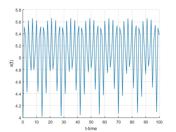
Figure 5. Graph of $x(t)$ for $x_{0}=4,P=2$ & $\delta=0.175$.

Conclusion: This study presents the evolution of population growth models and reasons for the need of models which are in the form of delay differential equations of pantograph type. Suitable transformation for the existing models have been proposed in this paper. It is generally difficult to obtain the analytic solutions of the population growth models which involve the delays. This paper shows innovative ways for obtaining the solution where other analytic methods fail. The solutions are presented in this paper to both the existing and modified models. The modified models which have been presented in this paper are generalized forms for some existing models which were obtained by taking cases. Stimulating procedures for finding patterns and regularities in seemingly chaotic processes have been elucidated. Population growth models for some of single and interacting species have been analyzed and illustrated by graphs. How, when, and why the changes in population sizes occur can be deduced from this study. This study provides information on effective ways for evaluating the impact of the physical environment on the species of organism and it can help to make accurate prediction on the population growth. This study can assist the conservation practitioners to evaluate the impact of the physical environment on a species and to determine whether the population in a given area will increase or decrease.

Acknowledgments: The first author acknowledges with thanks the postdoctoral fellowship and financial support from the DSI-NRF Center of Excellence in Mathematical and Statistical Sciences (CoE-MaSS). Opinions expressed and conclusions arrived are those of the authors and are not necessarily to be attributed to the CoE-MaSS.

References

- [1] S. Nickbakhsh, C. Mair, L. Matthews, R. Reeve, P. C. D. Johnson, F. Thorburn, B. Wissmann, A. Reynolds, J. McMenamin, R. N. Gunson, P. R. Murcia, Virus-virus interactions impact the population dynamics of influenza and the common cold, Proceedings of the National Academy of Sciences of the United States of America, 116 (52), (2019), 27142-27150.
- [2] D. S. Fischer, A. K. Fiedler, E. M. Kernfeld, R. M. J. Genga, A. Bastidas-Ponce, M. Bakhti, H. Lickert, J. Hasenauer, R. Maehr, F. J. Theis, Inferring population dynamics from single-cell RNA-sequencing time series data, Nat Biotechnol 37, (2019), 461-468.
- [3] S. Dong, F. Fan, Y. Huang, Studies on the population dynamics of a rumor-spreading model in online social networks, Physica A: Statistical Mechanics and its Applications, 492, (2018), 10-20.
- [4] R. Brady, H. Enderling, Mathematical Models of Cancer: When to Predict Novel Therapies, and When Not to, Bulletin of Mathematical Biology, 81, (2019), 3722-3731.
- [5] M. Tong , Z. Yan, L. Chao, (2020). Research on a Grey Prediction Model of Population Growth Based on a Logistic Approach. Discrete Dynamics in Nature and Society, Article ID 2416840, (2020).
- [6] S. S. Ezz-Eldien, On solving fractional logistic population models with applications, Computational and Applied Mathematics, 37, (2018), 6392-6409.
- [7] T. R. Malthus, An Essay on the Principle of Population, J. Johnson, London, England, (1798).
- [8] P.F. Verhulst, Notice sur la loi que la population poursuit dans son accroissement, Corresp. Math. Phys., 10 (1838), 113-121.
- [9] G. E. Hutchinson, Circular causal systems in ecology, Annals of the New York Academy of Sciences 50 (1948), 221-246.
- [10] F. Brauer, C. Castillo-Chavez, Mathematical models in population Biology and epidemiology, Texts in Applied Mathematics, Springer, New York, (2012).
- [11] M. Y. Dawed, P. R. Koya, A. Taye, Mathematical Modelling of Population Growth: The Case of Logistic and Von Bertalanffy Models, Open Journal of Modelling and Simulation, 2 (4), Article ID:49623, (2014).
- [12] J. Garca-Algarra, J. Galeano, J. M. Pastor, J. M. Iriondo, J. J. Ramasco, Rethinking the logistic approach for population dynamics of mutualistic interactions, Journal of Theoretical Biology 363, (2014), 332-343.
- [13] A. D. Polyanin, V. G. Sorokin, Nonlinear Pantograph-Type Diffusion PDEs: Exact Solutions and the Principle of Analogy, Mathematics 9, 511, (2021).
- [14] C. Hou, T. E. Simos, I. T. Famelis, Neural network solution of pantograph type differentialequations, Math Meth Appl Sci., 43, (2020), 3369-3374.
- [15] H. Jafari, N. A. Tuan, R. M. Ganji, A new numerical scheme for solving pantograph type nonlinear fractional integro-differential equations, Journal of King Saud University - Science, 33 (1), (2021), 101185.
- [16] A. Ali, K. Shah, T. Abdeljawad, H. Khan, A. Khan, Study of fractional order pantograph type impulsive antiperiodic boundary value problem, Advances in Difference Equations, 2020, Article number: 572 (2020).
- [17] Y. Liu, W. Chen, A new iterational method for ordinary equations using Sumudu transform, Advances in Analysis, 1 (2), (2016),89-94.
- [18] S. Vilu, R. R. Ahmad, U. K. Salma Din, Variational Iteration Method and Sumudu Transform for Solving Delay Differential Equation, International Journal of Differential Equations, 2019, Article ID 6306120, (2019).
- [19] M. O. Aibinu, S.C. Thakur, S. Moyo, Solving delay differential equations via Sumudu transform, International Journal of Nonlinear Analysis and Applications, (In Press), DOI: 10.22075/ijnaa.2021.22682.2402 (arXiv:2106.03515v1).
- [20] G. Wu, Challenge in the variational iteration method a new approach to identification of the Lagrange multipliers, Journal of King Saud University - Science, vol. 25, no. 2, (2013), 175-178.
- [21] G. Wu and D. Baleanu, Variational iteration method for fractional calculus a universal approach by Laplace transform, Advances in Difference Equations, vol. 2013, no. 1, (2013), 1-9.
- [22] G.K. Watugala, Sumudu transform a new integral transform to solve differential equations and control engineering problems, Mathematical Engineering in Industry, 24 (1), (1993), 35-43.
- [23] F. B. M. Belgacem, A. A. Karaballi, and S. L. Kalla, Analytical investigations of the Sumudu transform and applications to integral production equations, Mathematical Problems in Engineering, 3, (2003), 103-118.
- [24] F. B. M. Belgacem and A. Karaballi, Sumudu transform fundamental properties investigations and applications, Journal of Applied Mathematics and Stochastic Analysis, 2006, Article ID: 91083, (2006).
- [25] W. R. A. AL-Hussein, S. N. Al-Azzawi, Approximate solutions for fractional delay differential equations by using Sumudu transform method. In AIP Conference Proceedings, 2096 (1), (2019), 020007. AIP Publishing LLC.
- [26] A. K. Golmankhaneh, C. Tun, Sumudu transform in fractal calculus, Applied Mathematics and Computation, 350 (1), (2019), 386-401.
- [27] A .K. Alomari, M.I. Syam, N. R. Anakira, A. F. Jameel, Homotopy Sumudu transform method for solving applications in physics, Results in Physics, 18 (2020), 103265.
- [28] K. S. Nisar, A. Shaikh, G. Rahman, D. Kumar, Solution of fractional kinetic equations involving class of functions and Sumudu transform, Advances in Difference Equations, 2020, Article number: 39 (2020).
- [29] G. Adomian, A review of the decomposition method in applied mathematics, Journal of Mathematical Analysis and Applications, Vol. 135, no. 2, (1988), 501-544.
- [30] O. Arino, M.L. Hbid, E. Ait Dads, Delay Differential Equations and Applications, Springer, Marrakech, Morocco, (2002), 484-496.
- [31] W. S. C. Gurney, S. P. Blythe, R. M. Nisbet, Nicholson s blowflies revisited, Nature, 287 (5777), (1980), 17-21.