CPHT-RR113.122021

The Fate of Parisi-Sourlas Supersymmetry in Random Field Models

Abstract

By the Parisi-Sourlas conjecture, the critical point of a theory with random field (RF) disorder is described by a supersymmeric (SUSY) conformal field theory (CFT), related to a $d-2$ dimensional CFT without SUSY. Numerical studies indicate that this is true for the RF $\phi^{3}$ model but not for RF $\phi^{4}$ model in $d<5$ dimensions. Here we argue that the SUSY fixed point is not reached because of new relevant SUSY-breaking interactions. We use perturbative renormalization group in a judiciously chosen field basis, allowing systematic exploration of the space of interactions. Our computations agree with the numerical results for both cubic and quartic potential.

Introduction — Emergent symmetries are a frequent theme in modern theoretical physics. Such a symmetry is present at long distances but is not visible in the microscopic description of the system. A beautiful example is furnished by the physics of disordered systems, namely by the Random Field Ising Model (RFIM) and its cousins. Parisi and Sourlas suggested long ago Parisi and Sourlas (1979, 1981) that the critical points of these models obey emergent supersymmetry. While supersymmetry plays a prominent role in high-energy physics, its appearance in the statistical physics context came as a major surprise. A dramatic consequence of supersymmetry is dimensional reduction Aharony et al. (1976): the critical exponents of a disordered system in $d$ dimensions should be the same as those of the pure (i.e. non-disordered) system in $d-2$ dimensions.

Unfortunately, after 40 years of work, there is still no complete understanding whether, when, and how Parisi-Sourlas supersymmetry actually emerges. Most work focused on the random field $\phi^{4}$ and $\phi^{3}$ field theories, describing respectively the phase transition in RFIM and the statistics of Branched Polymers (BP) in a solution Lubensky and Isaacson (1979); Redner (1979); Gaunt (1980). Numerical studies of microscopic models suggest that supersymmetry and dimensional reduction are present in any dimension for the $\phi^{3}$ case Hsu et al. (2005) but only in sufficiently high $d$ for the $\phi^{4}$ case Fytas and Martín-Mayor (2013); Fytas et al. (2016, 2017, 2019). Why does this happen? One possibility is that some SUSY-breaking perturbations are dangerously irrelevant, i.e. irrelevant for high $d$, while become relevant at lower $d$ and break supersymmetry Brézin and De Dominicis (1998); Feldman (2002) . In this Letter we will report the first systematic exploration of this scenario. We will show that it gives a satisfactory unified description of phenomenology in agreement with all available numerical results .

The model and prior work — A random field (RF) model describes a statistical field theory with quenched disorder coupled to a local order parameter. We consider RF models of the type

$$\mathcal{S}[\phi,h]=\int d^{d}x\Big{[}\frac{1}{2}(\partial_{\mu}\phi)^{2}+V(\phi)+h(x)\phi(x)\Big{]}\,,$$ (1)

where $h(x)$ is drawn from a Gaussian distribution with zero mean and $\overline{h(x)h(0)}=H\delta(x)$ . Parisi-Sourlas (PS) conjecture Parisi and Sourlas (1979) about the critical points of these theories can be naturally divided in two parts:

1. Emergence of SUSY: The critical point of an RF theory is described by a special SUSY CFT (PS CFT).

2. Dimensional reduction: A large class of observables of the PS CFT (e.g. its critical exponents) are described by an ordinary CFT living in $\widehat{d}\equiv d-2$ dimensions.

While perturbatively valid for $d$ infinitesimally close to the upper critical dimension $d_{uc}$ (see below), this remarkable conjecture is known to sometimes fail for the physically interesting cases of integer $d<d_{uc}$.

As mentioned, the two most studied RF models are with $\phi^{4}$ (RFIM) and $\phi^{3}$ (BP) potentials. The RF $\phi^{4}$ model has a critical point in $3\leq d<d_{uc}=6$. PS conjecture would relate it to the usual Ising model in $\widehat{d}$ dimensions. Numerical studies Fytas and Martín-Mayor (2013); Fytas et al. (2016, 2017, 2019) show that while both SUSY and dimensional reduction hold in $d=5$, the conjecture fails in $d=4$. It also fails trivially for $d=3$, as the $\widehat{d}=1$ Ising model has no phase transition.

Similarly, the critical point of the RF $\phi^{3}$ model with imaginary coupling should be described by the usual Lee-Yang fixed point in $\widehat{d}$ dimensions Fisher (1978). BP critical exponent simulations suggest that this instance of PS conjecture works perfectly for any $2\leq d<d_{uc}=8$ Hsu et al. (2005) .

Let us come back to the central question of why PS conjecture sometimes works and sometimes fails. Many perturbative and non-perturbative arguments were given for Part 2 of the conjecture Parisi and Sourlas (1979); Cardy (1983); Klein and Perez (1983); Klein et al. (1984); Zaboronski (2002); Kaviraj et al. (2020). On the other hand Part 1 appears to be on less solid grounds. Here we will focus on the scenario Brézin and De Dominicis (1998); Feldman (2002) that Part 1 may fail due to dangerously invariant SUSY-breaking interactions.

From replicas to Cardy fields — We start by using the usual replica method where we take $n$ copies of the action (1) and average out the disorder. This gives the replica action:

$$\mathcal{S}_{n}=\int\!d^{d}x\Big{[}\sum_{i=1}^{n}\big{[}(\partial_{\mu}\phi_{i})^{2}+V(\phi_{i})\big{]}-\frac{H}{2}\big{(}\sum_{i=1}^{n}\phi_{i}\big{)}^{2}\Big{]}$$ (2)

from which one can get quenched averaged correlations functions $\overline{{\langle A(\phi)\rangle}}$ in $n\to 0$ limit by simply computing ${{\langle A(\phi_{1})\rangle}}$ having a single replica field.

We next apply Cardy’s linear field transform Cardy (1985):

$$\varphi=\frac{1}{2}(\phi_{1}+\rho)\,,\ \ \omega=\phi_{1}-\rho\,,\ \ \chi_{i}\stackrel{{\scriptstyle i\neq 1}}{{=}}\phi_{i}-\rho\,,$$ (3)

with $\rho=\frac{1}{n-1}\sum_{i=2}^{n}\phi_{i}$ and the condition $\sum_{i=2}^{n}\chi_{i}=0$. Turning off interactions for now ($V=0$), the transformed Lagrangian takes the form

$${\mathcal{L}}^{\text{free}}=\partial_{\mu}\varphi\partial_{\mu}\omega-\frac{H}{2}\omega^{2}+\frac{1}{2}\sum_{i=2}^{n}(\partial_{\mu}\chi_{i})^{2}\,.$$ (4)

Here and below, because of the replica limit $n\to 0$, we are dropping all terms proportional to powers of $n$.

From (4) we read off the classical scaling dimensions of the Cardy fields: $[\varphi]=\frac{d}{2}-2,[\chi_{i}]=\frac{d}{2}-1,[\omega]=\frac{d}{2}$ . In contrast, the original replica fields $\phi_{i}$ do not even have a well-defined scaling dimension . Although not manifest in the Cardy field basis, the S_n symmetry is still present and in particular not spontaneously broken . It will play an important role below.

While RF criticality is often described in terms of special “zero-temperature fixed points” Bray and Moore (1985); Fisher (1986), Cardy transform puts it on the same footing as the more familiar non-disordered criticality. Using Cardy fields, we will be able perform the RG analysis for the RF models borrowing the standard Wilsonian methodology Wilson and Kogut (1974); Kleinert and Schulte-Frohlinde (2001).

Leaders and followers — Let us now turn the interactions back on, and see how the theory renormalizes. Lagrangian (2) contains the interaction $\sum_{i=1}^{n}V(\phi_{i})$. This can be written as a sum of basic S_n singlet interactions $\sigma_{k}\equiv\sum_{i=1}^{n}\phi_{i}^{k}$. In an exhaustive analysis, we will have to consider further interaction terms respecting the replica permutation symmetry S_n, since they will be generated by RG evolution Brézin and De Dominicis (1998). Examples of such allowed interactions are products of $\sigma_{k}$’s as well as interactions containing derivatives. We will classify S_n singlet interactions in the original fields of (2), and then transform them to the Cardy fields.

The simplest interaction is the mass term $\sigma_{2}$ which in Cardy fields reads $2\varphi\omega+\chi_{i}^{2}$ and has classical dimension $d-2$. Continuing at the cubic level, the operator $\sigma_{3}$ under Cardy transform becomes

$$\sigma_{3}=(3\varphi^{2}\omega+3\chi_{i}^{2}\varphi)+(\chi_{i}^{3})-\big{(}\frac{3}{2}\chi_{i}^{2}\omega\big{)}+\big{(}\frac{1}{4}\omega^{3}\big{)}\,,$$ (5)

where different terms have unequal classical dimensions: $\frac{3d}{2}-4$ for the first term, while the successive ones sit 1,2 and 3 units higher. This new effect is generic: any singlet operator $\mathcal{O}$ in Cardy fields can be written as

$$\mathcal{O}={\mathcal{O}}_{L}+{\mathcal{O}}_{F_{1}}+{\mathcal{O}}_{F_{2}}+\cdots\,,$$ (6)

where $[\mathcal{O}_{F_{i}}]=[\mathcal{O}_{L}]+i$, $i=1,2,\ldots$. We call the lowest dimension part $\mathcal{O}_{L}$ the ‘leader’, and $\mathcal{O}_{F_{i}}$ ‘followers’.

In the first part of a Wilsonian RG step, integrating out a momentum shell and lowering the momentum cutoff $\Lambda\to\Lambda/b$ ($b>1$), a singlet operator $\mathcal{O}$, if present in the effective action, renormalizes as a whole, i.e. only through the change of the overall coefficient: $g\mathcal{O}\to\tilde{g}\mathcal{O}$ . This is guaranteed by S_n symmetry. On the other hand, in the second part of an RG step, bringing the cutoff back up to its original value, which rescales the fields $\varphi,\chi_{i},\omega$ according to their classical dimensions, the followers rescale by different coefficients from the leader, suppressing their relative effect in the IR (i.e. at large $b$):

$${\mathcal{O}}_{L}+\sum\nolimits_{i}{\mathcal{O}}_{F_{i}}\to b^{-[{\mathcal{O}}_{L}]}\big{(}{\mathcal{O}}_{L}+\sum\nolimits_{i}{b^{-i}}{\mathcal{O}}_{F_{i}}\big{)}.$$ (7)

Hence, the RG flow in the IR is controlled by the leaders. This drastically reduces the number of interactions to consider: only operators in Cardy fields which can be written as a leader of an S_n singlet interaction are of interest. The RG relevance or irrelevance of the leader determines the fate of the whole interaction Kaviraj et al. (2021).

Keeping the free massless Lagrangian (4), the mass term, and the leader parts $(\sigma_{2})_{L}$ or $(\sigma_{3})_{L}$ of the $\phi^{3}$ or $\phi^{4}$ interactions, we get the two Lagrangians relevant for the description of the RF $\phi^{3}$ and $\phi^{4}$ models:

$${\mathcal{L}}^{\phi^{3}}_{L}={\mathcal{L}}^{\text{free}}+m^{2}(2\varphi\omega+\chi_{i}^{2})+\frac{g}{2}(\varphi^{2}\omega+\chi_{i}^{2}\varphi)\,,$$ (8)

$${\mathcal{L}}^{\phi^{4}}_{L}={\mathcal{L}}^{\text{free}}+m^{2}(2\varphi\omega+\chi_{i}^{2})+\frac{g}{12}(2\varphi^{3}\omega+3\chi_{i}^{2}\varphi^{2})\,.$$

The mass term $m^{2}$ is strongly relevant and should be tuned to reach the IR fixed point. The upper critical dimension in this approach is fixed simply from the marginality of the leading non-quadratic interaction, which gives the well-known values cited above: $d_{uc}=8$ for the $\phi^{3}$ and 6 for the $\phi^{4}$ models.

Eqs. (8) give the correct effective theory for the two models close to their upper critical dimension, i.e. for $d=d_{uc}-\epsilon$, $\epsilon\ll 1$. Indeed, one can check that in this case, no other S_n singlet interactions exist whose leaders would be relevant (and, for the $\phi^{4}$ case, respecting the extra $\mathbb{Z}_{2}$ symmetry). However, we should keep an open mind about what may happen for $\epsilon=O(1)$, as some irrelevant interactions may become relevant. This will be investigated below.

Emergence of SUSY — It is easy to see that both Lagrangians (8) have emergent SUSY Cardy (1985). Note that the $n-2$ fields $\chi_{i}$ appear quadratically in the Lagrangians. The associated partition function is given by a Gaussian integral which at $n\to 0$ is equal to that of $2$ anticommuting scalars $\psi,\bar{\psi}$. So we are allowed to replace $\chi_{i}\chi_{i}\to 2\psi\bar{\psi}$. Then both the above theories can be compactly written as

$$\mathcal{S}_{\text{susy}}=\int d^{d}xd\theta d{\bar{\theta}}\Big{[}-\frac{1}{2}\Phi\partial^{a}\partial_{a}\Phi+V(\Phi)\Big{]}\,,$$ (9)

where $V(\phi)=m^{2}\phi^{2}+\frac{g}{6}\phi^{3}$ for the cubic theory and $V(\phi)=m^{2}\phi^{2}+\frac{\lambda}{4!}\phi^{4}$ for the quartic. Here $\Phi(x,\theta,{\bar{\theta}})=\varphi+\theta\bar{\psi}+{\bar{\theta}}\psi+\theta{\bar{\theta}}\omega$ is a superfield depending on coordinates $x,\theta,{\bar{\theta}}$ parametrizing the superspace $\mathbb{R}^{d|2}$ with OSp$(d|2)$ supergroup symmetry (PS supersymmetry), and $\partial^{a}\partial_{a}$ is the super-Laplacian (index $a$ takes values $1,\ldots,d,\theta,{\bar{\theta}}$). In the IR, we get a further enhancement to a PS superconformal symmetry OSp$(d+1,1|2)$ Kupiainen and Niemi (1983). The fixed point of this theory is therefore a PS CFT.

We now briefly describe basic properties of PS CFTs and how they undergo dimensional reduction app Local operators in such theories are classified according to their superconformal dimension $\Delta$ and their OSp$(d|2)$ spin $\ell$. They are grouped in superconformal multiplets containing a superprimary operator $\mathcal{O}^{\bf a}_{\Delta\ell}$ (where ${\bf{a}}$ stands for $a_{1}a_{2}\dots$), annihilated by the special superconformal generator $K^{a}$, and its superdescendants such as $\partial_{a}\mathcal{O}^{\bf a}_{\Delta\ell}$ and higher superderivatives. $\mathcal{O}^{\bf a}_{\Delta\ell}$ can be expanded in components which have different conformal dimensions:

$${\mathcal{O}}^{\bf{a}}(y)=\underbrace{\mathcal{O}_{0}^{\bf{a}}(x)}_{\Delta}+\theta\underbrace{\mathcal{O}_{\theta}^{\bf{a}}(x)}_{\Delta+1}+\bar{\theta}\underbrace{\mathcal{O}_{\bar{\theta}}^{\bf{a}}(x)}_{\Delta+1}+\theta\bar{\theta}\underbrace{\mathcal{O}_{\theta\bar{\theta}}^{\bf{a}}(x)}_{\Delta+2}\,.$$ (10)

Dimensional reduction restricts correlators of a PS CFT to a $(d-2)$-dimensional bosonic subspace $\mathcal{M}_{\widehat{d}}\equiv\{y=(\widehat{x}^{\alpha},0,0,0,0),\widehat{x}\in\mathbb{R}^{\widehat{d}}\}$. In addition, one only considers PS CFT operators invariant under the subgroup OSp$(2|2)$ (super)rotating the directions orthogonal to $\mathcal{M}_{\widehat{d}}$. In general, restricting to a subspace gives a nonlocal theory. The nontrivial fact is that by restricting the OSp$(2|2)$-singlet sector of the SUSY theory, we get a local ${\widehat{d}}$-dimensional CFT living on $\mathcal{M}_{\widehat{d}}$ Kaviraj et al. (2020). The local conserved CFT${}_{\widehat{d}}$ stress tensor appears in this setup as the $\mathcal{T}_{0}$ component of the PS CFT superstress tensor $\mathcal{T}$.

The dimensionally reduced CFT${}_{\widehat{d}}$ has the global symmetry of the original PS CFT: trivial in the $\phi^{3}$ case and $\mathbb{Z}_{2}$ for $\phi^{4}$. We will naturally assume that this CFT${}_{\widehat{d}}$ is nothing but the ${\widehat{d}}$-dimensional critical point of the same theory without disorder : the Wilson-Fisher fixed point for $\phi^{4}$ Wilson and Fisher (1972) and the Lee-Yang fixed point for $\phi^{3}$ Fisher (1978). Dimensions of many operators in these familiar theories being well-known both perturbatively and, sometimes, non-perturbatively, we can then use dimensional reduction to infer dimensions of operators in the PS CFT.

The central question is whether any S_n singlet perturbation, while irrelevant for $\epsilon\ll 1$, may become relevant for $\epsilon=O(1)$ and destabilize the SUSY IR fixed point. As discussed above, this may be answered by perturbing the Lagrangians ${\mathcal{L}}_{L}$ in (8) by the leader terms of S_n singlet interactions, and computing their scaling dimensions (restricting to $\mathbb{Z}_{2}$ singlets for $\phi^{4}$ case). A priori there are many leaders to consider, which moreover may mix under RG. Below we will divide them into three classes: susy-writable (SW), susy-null (SN), and non-susy-writable (NSW), with a triangular mixing matrix. Namely SN operators can generate only SN under RG flow, SW can generate SW and SN, while NSW can generate all three classes.

Susy-writable (SW) leaders — These are invariant under $O(n-2)$ acting on the indices of the $\chi_{i}$ fields. These operators can be transformed to the SUSY field bases by the substitution $\chi_{i}\to\psi$ (hence the name). With abuse of language we will also refer as SW to the resulting Sp$(2)$-invariant operators. In addition, we require that the operator does not vanish after the substitution (if so it will be classified below as susy-null). Most low-lying leaders turn out to be SW. E.g. the leader of any S_n singlet $\sum_{i=1}^{n}A(\phi_{i})$ has the form $A^{\prime}(\varphi)\omega+\frac{1}{2}A^{\prime\prime}(\varphi)\chi_{i}^{2}$ which is SW. This can be written as the highest component $A_{\theta{\bar{\theta}}}(\Phi)$ of a scalar composite superfield $A(\Phi)$. More generally, SW leaders are always in the highest component of a superfield . They do not have to be scalars of OSp($d|2$), but only singlets of the subgroup $\text{SO}(d)\times\text{Sp}(2)$. These are obtained from a highest component $\mathcal{O}^{\bf a}_{\theta{\bar{\theta}}}$ by contracting all its ${\bf a}$ indices with the $\text{Sp}(2)$-metric i.e. by setting the indices to $\theta$ and ${\bar{\theta}}$ app .

The OSp$(d|2)$ tensor representations of ${\mathcal{O}}^{\bf{a}}$ are associated to Young tableaux (YT) $(\ell_{1},\ell_{2},\cdots)$ with $\ell_{i}$ boxes in $i$-th row. Indices along the rows (columns) are graded (anti)symmetrized and all supertraces removed. Graded symmetry and antisymmetry respectively mean ${\mathcal{O}}^{ab}=(-1)^{[a][b]}{\mathcal{O}}^{ba}$ and ${\mathcal{O}}^{ab}=-(-1)^{[a][b]}{\mathcal{O}}^{ba}$ where $[a]=0(1)$ if $a$ is bosonic (fermionic). These general facts combined with the above procedure of setting the indices to $\theta$ and ${\bar{\theta}}$ shows that SW leaders can only be obtained from operators in representations labelled by YT of the form $(2,2,\dots,2)$. SW leaders are thus in correspondence with the following superfields ${\mathcal{S}}_{\theta{\bar{\theta}}},{\mathcal{J}}^{\theta{\bar{\theta}}}_{\theta{\bar{\theta}}},{\mathcal{B}}^{\theta{\bar{\theta}},\theta{\bar{\theta}}}_{\theta{\bar{\theta}}},\dots$ where ${\mathcal{S}}$ is a scalar, ${\mathcal{J}}^{ab}$ a spin-two, and ${\mathcal{B}}^{ab,cd}$ a “box” operator in the YT $(2,2)$ representation where $(a,b)$ and $(c,d)$ are the graded-symmetric pairs. Representations with higher number of rows can also appear in generic $d$ but we do not consider them since they have large classical dimensions.

The above formal considerations have a neat practical consequence: dimensions of SW leaders $\mathcal{O}_{\theta{\bar{\theta}}}$ can be obtained by studying the respective operators $\widehat{\mathcal{O}}$ in the dimensionally reduced model using $\Delta_{\mathcal{O}_{\theta{\bar{\theta}}}}=\Delta_{\mathcal{O}}+2=\Delta_{\widehat{\mathcal{O}}}+2$ from (10). From here we see immediately that SW leaders originating from scalar and spin two PS CFT operators cannot destabilize the SUSY fixed point. Indeed in both dimensionally reduced models all scalars (besides the mass term which we tune to reach the fixed point) are irrelevant. Similarly all the spin two operators should not cross the stress tensor and thus are expected to remain irrelevant in any $d$ .

Separate analysis is needed for operators in the box representation. In the dimensionally reduced models, an infinite family of such operators can be written in terms of $\widehat{d}$-dimensional scalar field $\widehat{\phi}$ as

$$\widehat{B}^{(k)}_{\alpha\beta,\gamma\delta}\equiv\widehat{\phi}^{k-3}\left(\widehat{\phi}_{,\alpha\beta}\widehat{\phi}_{,\gamma\delta}\widehat{\phi}-\tfrac{2\widehat{d}}{\widehat{d}-2}\widehat{\phi}_{,\alpha}\widehat{\phi}_{,\beta}\widehat{\phi}_{,\gamma\delta}\right)_{Y}\,,$$ (11)

with $k\geq 3$. Greek letters denote $\mathbb{R}^{\widehat{d}}$ indices, and $Y$ indicates the box YT symmetrization, the two symmetric rows being $\alpha\beta$ and $\gamma\delta$. These are the lowest dimensional operators made of $k$ fields in such representation.

We computed their perturbative one-loop dimensions for the $\phi^{3}$ case Kaviraj and Trevisani (2022), following the standard $\epsilon$-expansion methodology Wilson and Kogut (1974); Kleinert and Schulte-Frohlinde (2001), while the $\phi^{4}$ case was considered previously in Kehrein and Wegner (1994). The results (classical dimension plus one-loop correction) are:

$$\Delta_{\mathcal{B}_{\theta{\bar{\theta}}}^{(k)}}=\begin{cases}\big{(}2k+6-\frac{k}{2}\epsilon\big{)}_{\text{cl}}+\frac{2k^{2}-5k-2}{6}\epsilon&(\phi^{3})\,,\\ \big{(}k+2-\frac{k}{2}\epsilon\big{)}_{\text{cl}}+\frac{(k-3)(3k+2)}{18}\epsilon&(\phi^{4})\,.\end{cases}$$ (12)

Importantly, all anomalous dimensions are positive (excluding the $k=3$ $\phi^{4}$ case which, as all odd $k$ for $\phi^{4}$, is unimportant since it does not respect $\mathbb{Z}_{2}$ symmetry).

Susy-null (SN) leaders — These are singlets under $O(n-2)$ (like the SW operators) and satisfy the property of vanishing under the $\chi\to\psi$ map by the Grassmann nature of $\psi$. A typical example is $(\chi_{i}^{2})^{2}\to(\psi\bar{\psi})^{2}=0$. These operators have restrictive mixing properties and can only generate operators of the same class under RG. We identified an infinite class of S_n singlets app

$$\mathcal{N}_{k}=\frac{2}{k-3}\left(\frac{\sigma_{2}\sigma_{k-2}}{k-2}-\frac{2\sigma_{1}\sigma_{k-1}}{k-1}\right)\,,$$ (13)

for $k=4,5,6,\dots$, which have SN leaders $(\mathcal{N}_{k})_{L}=\varphi^{k-4}(\chi_{i}^{2})^{2}$. The $k=4$ operator is the lowest dimensional SN leader overall, while $(\mathcal{N}_{k})_{L}$ is the lowest dimensional SN leader made of $k$ fields.

Unlike for SW leaders, we cannot use SUSY theory and dimensional reduction to infer the scaling dimensions of SN operators (since they vanish identically in SUSY fields). We compute them directly from action (8). Our Cardy field approach makes these computations methodologically straightforward, being analogous to the standard $\epsilon$-expansion Wilson and Kogut (1974); Kleinert and Schulte-Frohlinde (2001). We thus computed the leading anomalous dimension of operators (13). The resulting scaling dimensions (classical plus one-loop) are given by:

$$\Delta_{{(\mathcal{N}_{k})}_{L}}=\begin{cases}\big{(}2(k+2)-\frac{\epsilon}{2}k\big{)}_{\textrm{cl}}+\frac{6k^{2}-7k-48}{18}\epsilon&(\phi^{3}),\\ \big{(}k+4-\frac{\epsilon}{2}k\big{)}_{\textrm{cl}}+\frac{(k-4)(k+3)}{6}\epsilon&(\phi^{4}).\end{cases}$$ (14)

The one-loop correction is positive except for the $k=4$, $\phi^{4}$ case when it vanishes. Then, the first nonzero correction appears at two loops, and it is negative Kaviraj et al. (2021):

$$\Delta_{{(\mathcal{N}_{4})}_{L}}=(8-2\epsilon)_{\textrm{cl}}-\frac{8}{27}\epsilon^{2}\quad(\phi^{4})\,.$$ (15)

Non-susy-writable (NSW) leaders — These operators are singlets under the S_n-1 that permutes the fields $\chi_{i}$, but not under $O(n-2)$, and therefore they cannot be mapped to $\psi,\bar{\psi}$ fields. A typical example would be any leader involving $\sum_{i=2}^{n}\chi_{i}^{3}$. In the RG flow, leader perturbations belonging to this class can generate perturbations from the other two classes, while the opposite mixing is forbidden by SUSY.

We investigated two infinite families of S_n singlets having NSW leaders app . The first family, first discussed by Feldman Feldman (2002) and in Kaviraj et al. (2021), is given by

$$\mathcal{F}_{k}=\sum_{i,j=1}^{n}(\phi_{i}-\phi_{j})^{k}=\sum_{l=1}^{k-1}(-1)^{l}\binom{k}{l}\sigma_{l}\sigma_{k-l}\,,$$ (16)

with $k=6,8,10,\dots$ . They give rise to NSW leaders made only of $\chi$ fields, of the form

$$\left(\mathcal{F}_{k}\right)_{L}=\sum_{l=2}^{k-2}(-1)^{l}\binom{k}{l}(\chi^{l}_{i})\left(\chi^{k-l}_{j}\right)\,,$$ (17)

The first leader of this family, $(\mathcal{F}_{6})_{L}$, is the lowest dimensional NSW leader overall.

The second family consists of S_n singlets given by

$$\mathcal{G}_{k}\equiv\frac{\sigma_{3}\sigma_{k-3}}{3(k-5)}+\frac{\sigma_{1}\sigma_{k-1}}{k-1}-\frac{(k-4)\sigma_{2}\sigma_{k-2}}{(k-5)(k-2)}\,,$$ (18)

for $k=6,7,8,\dots$. These have NSW leaders

$$(\mathcal{G}_{k})_{L}={\textstyle\frac{(k-4)(k-3)}{36}}\varphi^{k-6}\bigl{[}2(\chi_{i}^{3})^{2}-3(\chi_{i}^{2})(\chi_{j}^{4})\bigr{]},$$ (19)

The two families start from the same operator ($\mathcal{G}_{6}\propto\mathcal{F}_{6}$), but the higher operators are different. In fact $(\mathcal{G}_{k})_{L}$ is the lowest NSW leader made of $k$ fields, and in particular sits lower than $(\mathcal{F}_{k})_{L}$ for $k>6$.

Like for the SN class, we computed NSW scaling dimensions by the $\epsilon$-expansion methodology adapted to action (8). Starting with the $\mathcal{F}_{k}$ family, the scaling dimension (classical plus the leading correction) is given by

$$\Delta_{{(\mathcal{F}_{k})}_{L}}=\begin{cases}\big{(}3k-\frac{k}{2}\epsilon\big{)}_{\textrm{cl}}+\frac{2k^{2}-3k}{18}\epsilon&(\phi^{3}),\\ \big{(}2k-\frac{k}{2}\epsilon\big{)}_{\textrm{cl}}-\frac{k(3k-4)}{108}\epsilon^{2}&(\phi^{4}).\end{cases}$$ (20)

Notably, the leading anomalous dimension is one-loop and positive in the $\phi^{3}$ case Kaviraj and Trevisani (2022) while it is two-loop and negative for $\phi^{4}$ Feldman (2002); Kaviraj et al. (2021).

Considering next the $\mathcal{G}_{k}$ family, we obtained

$$\Delta_{{(\mathcal{G}_{k})}_{L}}=\begin{cases}\big{(}2(k+3)-\frac{k}{2}\epsilon\big{)}_{\textrm{cl}}+\frac{6k^{2}-7k-120}{18}\epsilon&(\phi^{3})\\ \big{(}k+6-\frac{k}{2}\epsilon\big{)}_{\textrm{cl}}+\frac{(k-6)(k+5)}{6}\epsilon\,.&(\phi^{4})\end{cases}$$ (21)

The one-loop correction is therefore always positive, except in the $k=6$, $\phi^{4}$ case when it vanishes. In the latter case, using $\mathcal{G}_{6}\propto\mathcal{F}_{6}$ and Eq. (20), we see that the leading, negative, correction appears at two loops.

Does SUSY emerge at $\epsilon=O(1)$? — The analysis leading to SUSY was based on the effective Lagrangians (8). It would be invalidated if a new relevant leader interaction is found in the IR. Allowed by symmetry, such a growing perturbation will be generated by the RG, destabilizing the flow and leading it away from the SUSY fixed point. Let us see if this scenario is realized.

Above we discussed several infinite families of leader interactions from three different classes (SW, SN, NSW). We will now focus on the lowest dimensional operators for each class. We expect them to be most important to decide the stability of the SUSY fixed point. First of all, $\epsilon$-expansion computations of lowest-dimensional operators should be more reliable than for higher-dimensional ones . Second, we expect crossing of operator dimensions (within the same mixing class) to be avoided nonperturbatively.

With this in mind we find that the SUSY IR fixed point of the RF $\phi^{3}$ theory should always be stable, since the lowest leader perturbations $\mathcal{B}_{\theta{\bar{\theta}}}^{(3)}$, $\mathcal{N}_{4}$, $\mathcal{F}_{6}$ never become relevant. To see this we take their one-loop dimensions given in Eqs. (12),(14),(20) and use these expressions in the full range of interest $2\leq d<8$ .

However, the same argument for the $\phi^{4}$ case reaches a different conclusion Kaviraj et al. (2021). While $\mathcal{B}_{\theta{\bar{\theta}}}^{(4)}$ remains irrelevant , both $(\mathcal{N}_{4})_{L}$ and $(\mathcal{F}_{6})_{L}$ become relevant at some critical dimension $d_{c}$ between four and five, namely $\Delta_{(\mathcal{N}_{4})_{L}}=d$ at $d=d_{c}\approx 4.6$ while $\Delta_{(\mathcal{F}_{6})_{L}}=d$ when $d_{c}\approx 4.2$. The precise value of $d_{c}$, and which of the two operators crosses marginality first, should be taken with a grain of salt coming from a two-loop computation. We may estimate the uncertainty replacing the expressions in Eqs. (15),(20) by their $\textrm{Pad\'{e}}_{[1,1]}$ rational approximants. We then find that $(\mathcal{N}_{4})_{L}$ crosses marginality at $d_{c}\approx 4.7$, while $(\mathcal{F}_{6})_{L}$ at $d_{c}\approx 4.5$.

NSW interaction $(\mathcal{F}_{6})_{L}$ clearly breaks SUSY. Operator $(\mathcal{N}_{4})_{L}$ is also potentially SUSY-breaking, by affecting NSW coupling evolution (while being SN it does not directly affect SW sector). We thus conclude that SUSY will be present in the RF $\phi^{4}$ model for $d_{c}<d<6$, while it will be lost for $d<d_{c}$ .

Remarkably, our findings exactly match the expectations from numerical studies mentioned at the beginning, for both universality classes. It is encouraging that already the leading order $\epsilon$-expansion results lead to this agreement. In the future, it would be interesting to determine our $d_{c}$ more accurately. This can be done systematically, increasing the perturbative order and using Borel resummation techniques, as is standard for the usual Wilson-Fisher fixed point Guida and Zinn-Justin (1998); Kleinert and Schulte-Frohlinde (2001); Kompaniets and Panzer (2017); Kompaniets and Wiese (2020).

Finally, we wish to compare our results to functional renormalization group studies of the RF $\phi^{4}$ model, which also predict the loss of SUSY for $d<d_{c}^{FRG}\approx 5.1$ Tissier and Tarjus (2012). While their $d_{c}$ is similar, their mechanism is quite different from ours, being attributed to fixed point annihilation Balog et al. (2020), so that below $d_{c}$ the SUSY fixed point does not exist. On the contrary, our SUSY fixed point exists for any $d$, being simply RG unstable for $d<d_{c}$. If so, one should be able to detect SUSY in lattice simulations for $d=4$, by performing additional tuning . This would be a decisive confirmation for our scenario.

A.K. is supported by DFG (EXC 2121: Quantum Universe, project 390833306), and E.T. by ERC (Horizon 2020 grant 852386). Simons Foundation grants 488655, 733758, and an MHI-ENS Chair also supported this work. We thank Kay Wiese for comments.

Appendix A PS SUSY and dimensional reduction

In the main text we had introduced the Parisi-Sourlas (PS) CFT as the IR fixed point of the supersymmetric theory in (9). At the IR fixed point supersymmetry is enhanced to a superconformal symmetry. This enhancement is a supersymmetric counterpart to the familiar emergence of conformal symmetry at the fixed points of non-supersymmetric models (see Nakayama (2015) for a review). In the main text we also discussed that there is a dimensional reduction from the PS SUSY CFT to a CFT${}_{\widehat{d}}$. In this appendix we clarify how the PS CFT is a simple generalisation of a usual CFT, which allows a straightforward extension of the usual CFT axioms to the SUSY case. Based on that, we provide some details on how a restricted sector of the theory defines a local CFT in $\widehat{d}$ dimension. The purpose of this appendix, based on Kaviraj et al. (2020), is to familiarize the reader with the concept of PS CFT.

A.1 PS CFT

Recall that to write the SUSY theory (9) in a compact way we had introduced the superspace coordinate $y^{a}\equiv(x^{\mu},\theta,{\bar{\theta}})$. Here $x^{\mu}\in\mathbb{R}^{d}$ are usual bosonic coordinates while $\theta,{\bar{\theta}}$ are Grassmann-valued (anticommuting) coordinates. The superspace index $a$ takes values $1,\dots d,\theta,{\bar{\theta}}$ while $\mu=1,\dots,d$. The OSp$(d|2)$ symmetry preserves the superspace distance $y^{a}y^{b}(g_{d|2})_{ab}$. Here the superspace metric is a natural extension of usual flat space metric, given by

$$(g_{d|2})_{ab}\equiv\left(\begin{array}[]{c c}g_{d}&0\\ 0&\frac{2}{H}g_{\textrm{Sp}(2)}\\ \end{array}\right)\ ,\quad g_{d}\equiv\mbox{diag}(\overbrace{1,1,\dots,1}^{d})\ .\quad g_{\textrm{Sp}(2)}\equiv\left(\begin{array}[]{c c}0&-1\\ 1&0\\ \end{array}\right)\,.$$ (26)

The trace of the metric is computed as ${\rm tr~{}}g_{d|2}\equiv(g_{d|2})_{a}^{\phantom{a}a}=d-2$ (notice that ${\rm tr~{}}g_{2|2}=0$). Derivatives in superspace are defined as $\partial_{a}\equiv\{\partial_{\mu},\partial_{\theta},\partial_{{\bar{\theta}}}\}$ and therefore the super-Laplacian of equation (9) takes the form $\partial^{a}\partial_{a}=\partial^{\mu}\partial_{\mu}-H\partial_{\theta}\partial_{{\bar{\theta}}}$.

The generators of the supersymmetry are simple extensions of usual Poincaré symmetry and they generate supertranslations ($P^{a}$) and superrotations ($M^{ab}$). Here $P^{\mu}$ and $M^{\mu\nu}$ are the usual ones, while $P^{\theta}$, $P^{\bar{\theta}}$, $M^{\mu\theta}$, $M^{\mu{\bar{\theta}}}$, $M^{\theta{\bar{\theta}}}$ are new generators. $P^{\theta}$, $P^{\bar{\theta}}$ are supertranslaton generators while $M^{\mu\theta}$, $M^{\mu{\bar{\theta}}}$ rotate bosonic into fermionic coordinates and are naturally called superotations.

At the fixed point the theory has the superconformal symmetry of OSp$(d+1,1|2)$. This is again a simple extension of the usual conformal group $SO(d+1,1)$, where we get the extra generators: superdilations $D$ and special superconformal transformations $K^{a}$, given by:

$$D=-y^{a}\partial_{a},\quad K^{a}=2y^{a}y^{b}\partial_{b}-y^{b}y_{b}\partial_{a}\,.$$ (27)

These expressions are thus very similar to the familiar expressions of the usual bosonic conformal symmetry, although note that superconformal $K^{\mu}$ does not reduce to the bosonic $K_{\rm bos}^{\mu}=2y^{\mu}y^{\nu}\partial_{\nu}-y^{\nu}y_{\nu}\partial_{\mu}$.

The algebra of generators is also similar to that of the conformal algebra $SO(d+1,1)$ but given in terms of graded-commutator $[X,Y\}$ - which is an anticommutator $\{X,Y\}$ if the two generators $X$ and $Y$ involve only the fermionic part of the group, otherwise a commutator $[X,Y]$. E.g. one has $[D,P^{a}\}=P^{a}$. The explicit forms of all these generators and their algebra are given in section 3.1 of Kaviraj et al. (2020).

In the main text we mentioned that local operators in PS CFT are classified by two labels $\Delta$ and $\ell$. We already discussed on p. The Fate of Parisi-Sourlas Supersymmetry in Random Field Models of the main text how OSp tensors with spin $\ell$ are defined and associated to a Young tableaux. An exhaustive discussion on the structure of OSp tensors can be found in section 3.1 of Kaviraj et al. (2020). It is also clear that one can associate to local operators a superconformal dimension $\Delta$ according to how they transform under superdilations, quite analogous a usual CFT.

In the SUSY CFT one naturally extends the notion of primaries and descendants. A SUSY operator $\mathcal{O}$ is superprimary if it satisfies $[K^{a},\mathcal{O}(0)\}=0$, or a superdescendant if it is related to a primary by the action of $P^{a}$. A superprimary and its superdescendants are grouped into a superconformal multiplet. Note that this multiplet may contain more than one operators that are usual primaries, but only one of them is a superprimary and rest are superdescendants.

Superconformal symmetry strongly restricts correlation functions. Their functional form matches the one of usual CFT_d, provided that points in $\mathbb{R}^{d}$ are uplifted to superspace $\mathbb{R}^{d|2}$. E.g. scalar 2-point functions are fixed as $\langle\mathcal{O}_{i}(y)\mathcal{O}_{j}(0)\rangle=\delta_{ij}(y^{2})^{-\Delta}$. Similarly the scalar 3-point functions are fixed up to OPE coefficients $\lambda_{ijk}$ as

$$\langle\mathcal{O}_{1}(y_{1})\mathcal{O}_{2}(y_{2})\mathcal{O}_{3}(y_{3})\rangle=\lambda_{123}|y_{12}|^{-\Delta_{1}-\Delta_{2}+\Delta_{3}}|y_{13}|^{-\Delta_{1}-\Delta_{3}+\Delta_{2}}|y_{23}|^{-\Delta_{2}-\Delta_{3}+\Delta_{1}}\,,$$ (28)

where $y_{ij}\equiv y_{i}-y_{j}$. The Operator Product Expansion (OPE) is also akin to the usual one e.g. for scalar operators ${\mathcal{O}}_{i}$ it schematically reads

$$\mathcal{O}_{1}(y)\mathcal{O}_{2}(0)\sim\lambda_{12{\mathcal{O}}}\frac{y_{a_{1}}\cdots y_{a_{\ell}}\mathcal{O}^{a_{1}\dots a_{\ell}}_{\Delta\ell}(0)}{|y|^{\Delta_{1}+\Delta_{2}-\Delta+\ell}}+\text{superdescendants}\,,$$ (29)

where we focused on the contribution of a single superprimary and its superdescendants. Using the OPE, a 4-point function can be expanded in superconformal blocks $G^{d}_{\Delta\ell}$ which correspond to the exchange of the supermultiplets of $\mathcal{O}_{\Delta\ell}$ in the OPE above. A more general discussion on 2- and 3-point functions of SUSY operators and superconformal blocks can be found in section 3.2 of Kaviraj et al. (2020). Our discussion above should hopefully convince the reader that PS CFTs satisfy very similar rules compared to the usual CFTs.

There is however one frequently used rule–unitarity–which does not hold. PS CFTs are necessarily nonunitary, since they violate spin-statistics relation, having anticommuting fields transforming in scalar rather than spinor representations of SO$(d)$. One should not be surprised that the PS CFT is non-unitary, as we have obtained it be taking the zero degree of freedom limit $n\to 0$. Of course unitarity is not a crucial relation from the point of view of statistical physis, and many statistical physics models are known to be non-unitary, PS CFT being just one more example. Being non-unitary, PS CFT is allowed to contain operators with dimensions below unitarity bounds, $\varphi$ being prime example, of classical scaling dimension $d/2-2$.

A.2 Dimensional reduction

Below Eq. (10) of the main text we discussed that a PS SUSY CFT can be dimensionally reduced to a local CFT${}_{\widehat{d}}$. Here we will explain this procedure in more detail. Dimensional reduction proceeds as follows. We take any correlator of SUSY operators $\mathcal{O}_{i}(y_{i})$ and restrict $y_{i}$ to the $(d-2)$-dimensional bosonic subspace $\mathcal{M}_{\widehat{d}}$ (see the main text). When we do this, the restricted correlator can be interpreted as a correlator of operators $\widehat{\mathcal{O}}_{i}(\widehat{x}_{i})$ of a $\widehat{d}$-dimensional CFT with $\widehat{x}_{i}\in\mathbb{R}^{\widehat{d}}$:

$$\langle\widehat{\mathcal{O}}_{1}(\widehat{x}_{1})\cdots\widehat{\mathcal{O}}_{n}(\widehat{x}_{n})\rangle=\langle\mathcal{O}_{1}(y_{1})\cdots\mathcal{O}_{n}(y_{n})\rangle\big{|}_{\mathcal{M}_{\widehat{d}}}\,.$$ (30)

In the usual CFT context, the procedure of restricting correlators to a subspace is sometimes referred to as ‘trvial defect’, where the word trivial is referred to the fact that we are not introducing any new degrees of freedom living on the defect, unlike for more nontrivial situations such as interfaces, nor are we introducing any nontrivial boundary conditions nor monodromies around the defect. We are just restricting correlators to the subspace. This procedure breaks the symmetry to SO$(d-1,1)\times\text{OSp}(2|2)$. The SO$(d-1,1)$ in the product is recognized as the conformal symmetry of the restricted CFT${}_{\widehat{d}}$, while OSp$(2|2)$ plays the role of a global symmetry.

We will next get rid of the additional OSp$(2|2)$ symmetry. We want to do this for two reasons. First of all we don’t expect a generic $\widehat{d}$-dimensional CFT to have such a symmetry. Second, as we will see below, getting rid of this extra symmetry is crucial to ensure that the dimensionally reduced theory is a local $\widehat{d}$-dimensional theory. This latter point is nontrivial as trivial defects normally give rise to nonlocal theories, i.e. theories without a local conserved stress tensor.

A natural way to accomplish this is to impose the additional requirement that operators $\mathcal{O}_{i}$ of the PS CFT in the above procedure should be singlets under OSp$(2|2)$. The restricted operators $\widehat{\mathcal{O}}_{i}$ are then also singlets. We thus got rid of OSp$(2|2)$ symmetry, as it now acts trivially on all kept operators.

To understand this construction consider the example of a rank 2 tensor superprimary ${\mathcal{O}}_{ab}$. Before restricting it to $\mathcal{M}_{\widehat{d}}$, we should convert it to an OSp$(2|2)$ singlet. This can be done contracting it with the $\widehat{d}$ dimensional metric $g_{\widehat{d}}^{ab}$, as follows:

$${\mathcal{O}}_{ab}\to g_{\widehat{d}}^{ca}g_{\widehat{d}}^{db}{\mathcal{O}}_{ab}\,.$$ (31)

This amounts to setting the $a,b$ indices to $\widehat{d}$-dimensional indices inside $\mathcal{M}_{\widehat{d}}$.

There are other ways to get OSp$(2|2)$ singlet from ${\mathcal{O}}_{ab}$, which involve contracting ${\mathcal{O}}_{ab}$ or its derivatives with the metric $g_{2|2}^{ab}$, e.g.

$$g_{2|2}^{ab}{\mathcal{O}}_{ab}\,,\;\partial^{a}_{\perp}\partial^{b}_{\perp}{\mathcal{O}}_{ab}\,,\;g_{\widehat{d}}^{ca}\partial^{b}_{\perp}{\mathcal{O}}_{ab}\,,\;g_{\widehat{d}}^{ca}g_{\widehat{d}}^{db}\partial^{2}_{\perp}{\mathcal{O}}_{ab}\,,\;g_{\widehat{d}}^{ca}\partial^{b}_{\perp}(\partial^{2}_{\perp})^{2}{\mathcal{O}}_{ab}\,,\dots\,.$$ (32)

Here $\partial_{\perp}$ denotes derivatives along directions orthogonal to ${\mathcal{M}}_{\widehat{d}}$: $\partial^{a}_{\perp}=g_{2|2}^{ab}\partial_{b}$.

Now, a crucial fact is that any OSp$(2|2)$ singlet correlator involving one or more operators of the type (32) vanishes when restricted to $\mathcal{M}_{\widehat{d}}$. This happens because the restriction involves objects like the $g_{2|2}^{ab}$ metric contracted with $\widehat{x}^{\mu}$ (coordinates on $\mathcal{M}_{\widehat{d}}$) or $g_{2|2}^{ab}$ contracted with another $g_{2|2}^{ab}$. All of such contractions are however zero (in particular the supertrace of $g_{2|2}$ is zero). In Kaviraj et al. (2020) the singlets of the type shown in (31) were called $S_{0}$ operators while the second type i.e. (32) as $S_{1}$. What we are saying is that if we focus on restricted correlators of $S_{0}$, all $S_{1}$ operators decouple.

To summarize, in dimensional reduction nontrivial operators $\widehat{\mathcal{O}}$ of the reduced theory are $S_{0}$ singlets obtained from SUSY operators ${\mathcal{O}}$. The precise form of the map $\mathcal{O}\to\widehat{\mathcal{O}}$ for a general tensor operator is discussed in section 4.1 of Kaviraj et al. (2020).

The decoupling of $S_{1}$ operators allows us to define a stress tensor $\widehat{T}^{\alpha\beta}$ of the CFT${}_{\widehat{d}}$ from the super-stress tensor $\mathcal{T}^{ab}$ of the PS CFT. One can write $\widehat{T}^{\alpha\beta}(\widehat{x})=\mathcal{T}^{\{\alpha\beta\}}_{0}(\widehat{x})$ where $\{\}$ opportunely removes SO$(\widehat{d})$-traces, which are $S_{1}$ operators. The super-stress tensor has the superconformal dimension $d-2$ which follows from its superconservation equation (these properties of $\mathcal{T}$ are discussed in detail in section 3.2 and App. C of Kaviraj et al. (2020)). As a consequence $\widehat{T}$ also has dimension $\widehat{d}$. Note that it also has SO$(\widehat{d})$-spin two. This already indicates that it is a conserved stress stensor in CFT${}_{\widehat{d}}$. To motivate this further, one can easily see that it is conserved up to $S_{1}$ operators, namely $0=\partial_{a}\mathcal{T}_{0}^{a\beta}=\partial_{\alpha}\widehat{T}^{\alpha\beta}+S_{1}$. Thus if the PS CFT is local, the reduced theory is also local. For a detailed proof of this conservation equation and a discussion of Ward identities see section 4.3 of Kaviraj et al. (2020).

It should be clear by now how a reduced local CFT is defined from the PS SUSY CFT. To give a more complete picture of the CFT${}_{\widehat{d}}$, we will now show the operator product expansion (OPE) of reduced theory operators. We will see below that this leaves us with some nice consequences. Let us take the superfield OPE (29). We focus on $S_{0}$ type singlets and restrict the OPE to ${\mathcal{M}}_{\widehat{d}}$. Then it takes a very simple form:

$$\!\!\!\widehat{\mathcal{O}}_{1}(\widehat{x})\widehat{\mathcal{O}}_{2}(0)\sim\lambda_{12{\mathcal{O}}}\dfrac{\widehat{x}_{\alpha_{1}}\cdots\widehat{x}_{\alpha_{\ell}}\widehat{\mathcal{O}}^{\alpha_{1}\dots\alpha_{\ell}}_{\Delta\ell}(0)}{|\widehat{x}|^{\Delta_{1}+\Delta_{2}-\Delta+\ell}}+\text{descendants}+S_{1}\,,$$ (33)

where, for each superprimary $\mathcal{O}_{\Delta\ell}$ exchanged in (29), there is in (33) a unique operator $\widehat{\mathcal{O}}_{\Delta\ell}$ of $S_{0}$ type with the same $\Delta,\ell$ and $\lambda_{12{\mathcal{O}}}$ as in (29). The other infinitely many primaries are $S_{1}$ and thus decouple when the OPE is used in OSp$(2|2)$-invariant corrrelators. This leads to a remarkable fact: OSp$(d+1,1|2)$ superconformal blocks are equal to SO$(d-1,1)$ conformal blocks i.e. $G_{\Delta\ell}^{d}=g_{\Delta\ell}^{d-2}$. This equality has another beautiful consequence. Note that since a superconformal multiplet packages a finite number of $SO(d+1,1)$ primaries, a superconformal block can be decomposed into a finite number of usual CFT_d blocks. We can thus write a CFT_d-2 block as a finite combination of CFT_d blocks. This recursion relation is elaborately discussed in section 4.4 of Kaviraj et al. (2020).

Appendix B Susy-writable (SW) leaders

Here we will explain statements about the SW leaders made in the main text and provide some examples. The goal is to make the reader comfortable with this concept.

As defined on p. The Fate of Parisi-Sourlas Supersymmetry in Random Field Models in the main text, SW leaders are those leader operators which 1) can be mapped to $\psi,\bar{\psi}$ fields and 2) do not vanish after such a map. The first of these conditions means that the operator can only involve $\chi_{i}$ fields or their derivatives with indices contracted in $O(n-2)$ invariant fashion. E.g. $\chi_{i}\chi_{i}$ or $\partial_{\mu}\chi_{i}\partial_{\mu}\chi_{i}$ can be mapped to $\psi,\bar{\psi}$, becoming, respectively, $2\psi\bar{\psi}$ and $2\partial_{\mu}\psi\partial_{\mu}\bar{\psi}$. An exhaustive discussion of such mapppings, including the origin of the factor 2, is in Appendix C of Kaviraj et al. (2021). On the other hand there is no way to map an operator $\sum_{i=2}^{n}\chi_{i}^{3}$ to $\psi,\bar{\psi}$ fields. Such a combination is only invariant under S_n-1 permuting the $\chi_{i}$’s but not under the $O(n-2)$ rotating them. Leaders containing such combinations of $\chi$’s do exist, and they are classified as non-susy-writable (NSW).

Certain operators can be mapped to $\psi,\bar{\psi}$ but vanishes under such a mapping due to the Grassmann nature of the fields. A typical example is $(\chi_{i}\chi_{i})^{2}$ which maps to zero because $\psi^{2}=\bar{\psi}^{2}=0$. Leaders having this property are classified not as SW but as susy-null (SN). SN operators have zero correlators among themselves and with any SW operator, but in general not with NSW operators. Hence we cannot just forget about SN leader perturbations, as they might backreact on NSW perturbations and thus, indirectly, destabilize the theory. Indeed, we dedicated a separate section in the main text to the SN leaders (more on this below).

The above definition of SW operators only defines them up to SN contributions. SW leaders with good scaling dimensions (at some order in perturbation theory) will usually be linear combinations of several monomials, some of which can be SN. This subtlety does not play a big role in classifying SW operators and in computing their anomalous dimensions. Under RG flow, SN and SW operators mix triangularly, as SW operators can RG-generate both SW and SN operators, while SN can only generate SN. Thus we can always set the SN part of SW operator to zero in all computations of SW anomalous dimensions.

Modulo SN operators, the map $\psi\leftrightarrow\chi$ is a bijection in the space of SW operators written in Cardy and in SUSY fields. So we will call SW also the operators in SUSY fields obtained after applying this map.

In the discussion of SW leaders in the main text, a key role was played by the fact that the $\chi\to\psi$ map maps them to the highest component of a superfield. This fact was conjectured and extensively checked in Kaviraj et al. (2021). A rigorous proof will be presented, for the first time, in App. B.1 below. Here we will provide some introductory comments, which should make the reader comfortable with this important property. As a first example, consider the S_n singlet operator of the form $\sum_{i=1}^{n}A(\phi_{i})$ which is mapped to Cardy fields as follows

$$\sum_{i=1}^{n}A(\phi_{i}) = A\left(\varphi+\frac{\omega}{2}\right)+\sum_{i=2}^{n}A\left(\varphi-\frac{\omega}{2}+\chi_{i}\right)=\bigg{\{}A^{\prime}(\varphi)\omega+\frac{1}{2}A^{\prime\prime}(\varphi)\sum_{i=2}^{n}\chi_{i}^{2}\bigg{\}}+\ldots\,.$$ (34)

To obtain the r.h.s of this equation we Taylor-expanded the central expression around $\varphi=0$. We then gathered terms of the lowest dimension in the curly brackets—this is the leader of the considered S_n singlet. One can easily check that all the terms $\ldots$ have a higher dimension—they are followers.

Applying the map $\chi\to\psi$ to the leader, we obtain $A^{\prime}(\varphi)\omega+A^{\prime\prime}(\varphi)\psi\bar{\psi}$. Note that this particular combination of fields is invariant under supertranslations transformations:

$$\delta\varphi=\bar{\varepsilon}\psi+\varepsilon\bar{\psi},\qquad\delta\psi=-\varepsilon\omega,\qquad\delta\bar{\psi}=\bar{\varepsilon}\omega,\qquad\delta\omega=0\,.$$ (35)

These are called supertranslations because they follow from considering how components of the superfield

$$\Phi(x,\theta,{\bar{\theta}})=\varphi(x)+\theta\bar{\psi}+{\bar{\theta}}\psi+\theta{\bar{\theta}}\omega$$ (36)

transform when applying translations in the fermionic coordinates $\theta,{\bar{\theta}}\to\theta+\varepsilon,{\bar{\theta}}+{\bar{\varepsilon}}$.

Invariance under supertranslations is a general property of the highest component $\mathcal{O}^{\textbf{a}}_{\theta{\bar{\theta}}}$ of any superfield $\mathcal{O}^{\textbf{a}}$ (see Eq. (10)). Since we found that the leader $A^{\prime}(\varphi)\omega+A^{\prime\prime}(\varphi)\psi\bar{\psi}$ is supertranslation invariant, it is natural to inquire of which superfield it is the highest component. It is easy to check that the answer is the composite superfield $A(\Phi)$, as stated in the main text.

The following additional reasoning may further convince the reader in the plausibility of the discussed property. According to the logic of our approach, leader operators under RG flow generate only leaders. When we specialize to SW leaders, this RG property of the leaders must be encoded in some special selection rule of the SUSY theory. Our claim is that this selection rule is precisely one based on supertranslation invariance.

An additional interesting twist of the story is as follows. The SW leader perturbations we are interested in are scalars under rotation, and they also preserve Sp$(2)$ symmetry rotating $\psi$ and $\bar{\psi}$ (this Sp$(2)$ symmetry descends from the $O(n-2)$ symmetry in the $\chi_{i}$ formulation, after the $n\to 0$ limit). In other words, they are SO$(d)\times$Sp$(2)$ invariant fields (although they do not need to respect full OSp$(d|2)$ invariance). As mentioned any such leader lives in the highest component $\mathcal{O}^{\textbf{a}}_{\theta{\bar{\theta}}}$ of a superfield $\mathcal{O}^{\textbf{a}}$. Note that this superfield does not have to be a scalar. If it is a scalar (no a indices), the leader is just $\mathcal{O}_{\theta{\bar{\theta}}}$. This was the case for the above example. If, on the other hand, the superfield is a tensor, the leader is obtained from $\mathcal{O}^{\textbf{a}}_{\theta{\bar{\theta}}}$ by contracting a indices with the Sp$(2)$ metric, which produces an SO$(d)\times$Sp$(2)$ invariant field as the leader should be. Effectively, to produce a leader we have to set a indices in the directions labelled by $\theta,{\bar{\theta}}$. Hopefully this explains better statements made in this respect in the main text. Notice that in principle the indices a could be contracted also with the SO$(d)$ metric, however this procedure does not generate new operators since $\mathcal{O}$ are supertraceless, which implies $\mathcal{O}^{\mu\mu}={\frac{4}{H}}\mathcal{O}^{\theta{\bar{\theta}}}$.

Let us consider some examples how this works for tensor superfields. One such superfield, of rank 2, is the superstresstensor $\mathcal{T}^{ab}$ which was defined in App. C of Kaviraj et al. (2020). Computing its highest component $\mathcal{T}_{\theta{\bar{\theta}}}^{ab}$ and setting $a=\theta,b={\bar{\theta}}$ we obtain

$$\mathcal{T}_{\theta{\bar{\theta}}}^{\theta{\bar{\theta}}}\propto\partial_{\mu}\varphi\partial_{\mu}\omega+\partial_{\mu}\psi\partial_{\mu}\bar{\psi}+{\frac{H}{2}(2-d)}\omega^{2}$$ (37)

This is clearly a SW leader, since it’s a linear combination of terms appearing in the quadratic part of the Parisi-Sourlas SUSY Lagrangian. In fact it is a linear combination of leaders of S_n singlets $\sigma_{1}^{2}$ and $\partial^{\mu}\phi_{i}\partial_{\mu}\phi_{i}$.

For a less trivial example, consider the superfield $\Phi^{2}\mathcal{T}^{ab}$. In this case the highest component contracted with Sp$(2)$, $(\Phi^{2}\mathcal{T}^{\theta{\bar{\theta}}})_{\theta{\bar{\theta}}}$ is a lengthy expression given in Eq. (8.13) of Kaviraj et al. (2021). It can be shown to be a linear combination of two dimension 8 leaders associated with $\sigma_{1}\sigma_{3}$ and $\sum_{i}\phi_{i}^{2}\partial_{\mu}\phi_{i}\partial_{\mu}\phi_{i}$.

Our final example is the Sp$(2)$-invariant part ${\mathcal{B}}^{\theta{\bar{\theta}},\theta{\bar{\theta}}}_{\theta{\bar{\theta}}}$ of the highest component ${\mathcal{B}}^{ab,cd}_{\theta{\bar{\theta}}}$ of the superfield ${\mathcal{B}}^{ab,cd}$ in the box $(2,2)$ representation. An infinite family of such composite superfields can be built from the fundamental superfield $\Phi$ by an immediate counterpart of the $\widehat{d}$-dimensional Eq. (11) in the main text:

$$({\mathcal{B}}^{(k)})^{ab,cd}\equiv{\Phi}^{k-3}\left(\Phi_{,ab}\Phi_{,cd}\Phi-\tfrac{2\widehat{d}}{\widehat{d}-2}\Phi_{,a}\Phi_{,b}\Phi_{,cd}\right)_{Y}\,.$$ (38)

From this equation, one can work out $({\mathcal{B}}^{(k)})^{\theta{\bar{\theta}},\theta{\bar{\theta}}}_{\theta{\bar{\theta}}}$ explicitly in terms of $\varphi$, $\psi$, $\bar{\psi}$ and $\omega$. For example, the full expression for $k=4$ is given in Eq. (H.5) of Kaviraj et al. (2021) and we do not copy it here. It is then possible to check that this expression is (up to total derivatives) a linear combination of SW leaders of the following S_n singlet operators: $\sigma_{1}^{2}\sigma_{2}$, $\partial_{\mu}\sigma_{1}\partial_{\mu}\sigma_{3}$, $\sigma_{1}\sum_{i}\phi_{i}\partial_{\mu}\phi_{i}\partial_{\mu}\phi_{i}$, $\sigma_{2}\sum_{i}\partial_{\mu}\phi_{i}\partial_{\mu}\phi_{i}$, $\sum_{i}\phi_{i}\partial_{\mu}\phi_{i}\partial_{\nu}\phi_{i}\partial_{\mu}\partial_{\nu}\phi_{i}$, $\sum_{i}\phi^{2}_{i}\partial_{\mu}\partial_{\nu}\phi_{i}\partial_{\mu}\partial_{\nu}\phi_{i}$. Leader tables from App. D of Kaviraj et al. (2021) are helpful when performing this check.

To summarize, in this appendix we explained in more detail how SW leaders are captured by the highest components of superfields (see App. B.1 for a rigorous proof). Since the superfield scaling dimensions can be found from the dimensionally reduced theory, this property drastically simplifies the task of computing SW leaders scaling dimensions. This is how it was used in the main text.

B.1 Correspondence between SW leaders and supertranslation invariant SUSY fields

For a SW leader $\mathcal{O}$, written in terms of Cardy fields, denote by $\mathcal{O}^{\prime}$ the corresponding operator mapped to SUSY fields by the $\chi\rightarrow\psi$ map. The operation $\mathcal{O}\rightarrow\mathcal{O}^{\prime}$ has two properties: 1) the resulting operator $\mathcal{O}^{\prime}$ is a supertranslation-invariant (st-invariant, for short) SUSY field; 2) any st-invariant and Sp(2) invariant field of the SUSY theory can be written as $\mathcal{O}^{\prime}$ for some SW leader $\mathcal{O}$. These facts were first noticed in Kaviraj et al. (2021) based on many examples, and conjectured to be always true. Here we will provide a rigorous proof that this is indeed the case.

B.1.1 Any SW leader maps to an st-invariant operator

The most general singlet interaction, in terms of replicated fields $\phi_{i}$, can be written as a linear combination of products of elementary singlet interactions, of the form

$$\sum_{i=1}^{n}A[\phi_{i}],$$ (39)

where $A[\phi]$ is a function of $\phi$ and its first, second,… derivatives, evaluated at point $x$. Some of the derivative indices may be contracted with each other, others when products of elementary interactions are taken. E.g. we may have $A[\phi]=\phi\partial_{\mu}\phi$.

Let us translate (39) to the Cardy fields. Generalizing Eq. (5.14) in Kaviraj et al. (2021) to the case when $A[\phi]$ may also depend on the derivatives, the lowest dimension part of the above singlet is given by

$$\int\frac{\delta A[\varphi](x)}{\delta\varphi(x_{1})}\omega(x_{1})dx_{1}+\frac{1}{2}\int\frac{\delta^{2}A[\varphi](x)}{\delta\varphi(x_{1})\delta\varphi(x_{2})}\chi_{i}(x_{1})\chi_{i}(x_{2})dx_{1}dx_{2}\,.$$ (40)

The $\chi\rightarrow\psi$ map maps this to (use App. C of Kaviraj et al. (2021), first Eq. (C.3), simplifying as $\frac{\delta^{2}A(x)}{\delta\varphi(x_{1})\delta\varphi(x_{2})}$ is symmetric in $x_{1},x_{2}$):

$$\mathcal{O}^{\prime}=\int\frac{\delta A(x)}{\delta\varphi(x_{1})}\omega(x_{1})dx_{1}+\int\frac{\delta^{2}A(x)}{\delta\varphi(x_{1})\delta\varphi(x_{2})}\psi(x_{1})\bar{\psi}(x_{2})dx_{1}dx_{2}\,.$$ (41)

Let us check that this is invariant under the supertranslations

$$\delta_{\operatorname{st}}\varphi=\bar{\varepsilon}\psi+\varepsilon\overline{\psi,}\quad\delta_{\operatorname{st}}\bar{\psi}=\bar{\varepsilon}\omega,\quad\delta_{\operatorname{st}}\psi=-\varepsilon\omega,\quad\delta_{\operatorname{st}}\omega=0\,.$$ (42)

Using $\delta_{\operatorname{st}}\frac{\delta A(x)}{\delta\varphi(x_{1})}=\int\frac{\delta^{2}A(x)}{\delta\varphi(x_{1})\delta\varphi(x_{2})}\delta_{\operatorname{st}}\varphi(x_{2})dx_{2}$ we get that $\delta_{\operatorname{st}}$ of the first term in $\mathcal{O}^{\prime}$ cancels with

$$\int\frac{\delta^{2}A(x)}{\delta\varphi(x_{1})\delta\varphi(x_{2})}\delta_{\operatorname{st}}[\psi(x_{1})\bar{\psi}(x_{2})]dx_{1}dx_{2}.$$ (43)

Let us show that the remaining part of $\delta_{\operatorname{st}}$ of the second term in $\mathcal{O}^{\prime}$,

$$\int\delta_{\operatorname{st}}\frac{\delta^{2}A(x)}{\delta\varphi(x_{1})\delta\varphi(x_{2})}\psi(x_{1})\bar{\psi}(x_{2})dx_{1}dx_{2}=\int\frac{\delta^{3}A(x)}{\delta\varphi(x_{1})\delta\varphi(x_{2})\delta\varphi(x_{3})}\psi(x_{1})\bar{\psi}(x_{2})[\bar{\varepsilon}\psi(x_{3})+\varepsilon\bar{\psi}(x_{3})],$$ (44)

vanishes. If $A$ is a function of only $\varphi$ and not of derivatives, then $\frac{\delta^{3}A(x)}{\delta\varphi(x_{1})\delta\varphi(x_{2})\delta\varphi(x_{3})}$ is proportional to delta functions, and (44) vanishes because of $\psi^{2}=0$, $\bar{\psi}^{2}=0$. When $A$ also depends on derivatives, $\frac{\delta^{3}A(x)}{\delta\varphi(x_{1})\delta\varphi(x_{2})\delta\varphi(x_{3})}$ will involve derivative of deltas. The important thing is that it is always symmetric in the interchanges of $x_{i}$. The first fermionic product in (44) is antisymmetric in $x_{1},x_{3}$ and the second in $x_{2},x_{3}$. So the integral will vanish.

The above argument shows that $\mathcal{O}^{\prime}$ is st-invariant. Products of $\mathcal{O}^{\prime}$’s will also be st-invariant. This proves st-invariance of all SW leaders of general singlets, since those can be obtained by taking linear combinations of products of different elementary singlet interactions of the form (39).

It may sometimes happen that two different singlet interactions give rise, through the above construction, to leaders which are either 1) exactly the same when written in the $\chi$ fields, or 2) becomes the same after $\chi\rightarrow\psi$. Then, taking their difference, we obtain an interaction whose leader is either susy-null (case 2), or non-susy-writable (case 1). E.g. in case 1 the leader will involve contributions of terms $\sum\chi_{i}^{k}$, $k\geqslant 3$, or their generalizations with derivatives, see Kaviraj et al. (2021), last line of (5.14). These terms cannot cancel because operators $\sum\chi_{i}^{k}$ are all algebraically independent. This shows that the leader will be NSW. So we need not be worried about such cancelations for the purposes of proving the result of this section.

B.1.2 Any Sp(2) and st-invariant operator comes from a SW leader

To prove this result, we take an arbitrary Sp(2) and st-invariant SUSY operator. We can write it as $(X)_{\theta\bar{\theta}}$, the $\theta\bar{\theta}$ component of a Sp(2) invariant superfield $X$. Being Sp(2) invariant, $X$ can be written as a linear combination of products of the fundamental superfield $\Phi$ and of its superderivatives, contracted with either SO$(d)$ metric $g_{\mu\nu}$ or with the Sp(2) metric $g_{ab}$. In what follows $a,b$ are Sp(2) indices: $a,b\in\{\theta,\bar{\theta}\}$.

Consider first the simplest case when $X$ only involves normal derivatives, contracted with $g_{\mu\nu}$. We can simplify this even further by considering a product of $K$ superfields at different points. We will call such special $X$’s by a letter $Y$:

$$Y=\Phi(x_{1})\ldots\Phi(x_{K})\,.$$ (45)

We will prove that $Y_{\theta\bar{\theta}}$ arises from an SW leader of a singlet. Differentiating with respect to $x_{k}$, and setting all ${x_{k}}$ equal, we can then obtain the statement for $X$’s involving derivatives in the $\mu$ directions.

Let us compute $Y_{\theta\bar{\theta}}$ for (45). We have

$$Y_{\theta\bar{\theta}} = \sum_{k}\Phi_{\theta\bar{\theta}}(x_{k})\prod_{l\neq k}\Phi_{0}(x_{l})+\sum_{k_{1}\neq k_{2}}\Phi_{\theta}(x_{k_{1}})\Phi_{\bar{\theta}}(x_{k_{2}})\prod_{l\neq k_{1}k_{2}}\Phi_{0}(x_{l})$$ (46)

$$= \sum_{k}\omega(x_{k})\prod_{l\neq k}\varphi(x_{l})+\sum_{k_{1}\neq k_{2}}\psi(x_{k_{1}})\bar{\psi}(x_{k_{2}})\prod_{l\neq k_{1}k_{2}}\varphi(x_{l})\,.$$

Consider the following S_n singlet:

$$\sum_{i}\phi_{i}(x_{1})\ldots\phi_{i}(x_{K})\,.$$ (47)

Mapping it to Cardy fields, we obtain the leader

$$\sum_{k}\omega(x_{k})\prod_{l\neq k}\varphi(x_{l})+\sum_{k_{1}\neq k_{2}}\sum_{i}\frac{1}{2}\chi^{i}(x_{k_{1}})\chi^{i}(x_{k_{2}})\prod_{l\neq k_{1}k_{2}}\varphi(x_{l})\,,$$ (48)

plus followers involving terms higher order in $\chi$. According to the dictionary of App. C of Kaviraj et al. (2021), the $\chi\rightarrow\psi$ map maps

$$\chi^{i}(x_{k_{1}})\chi^{i}(x_{k_{2}})\rightarrow\psi(x_{k_{1}})\bar{\psi}(x_{k_{2}})+\psi(x_{k_{2}})\bar{\psi}(x_{k_{1}})\,.$$ (49)

Thus we see that (48) maps precisely on (46). This proves that any $Y_{\theta\bar{\theta}}$ arises from an SW leader of a singlet. As mentioned above, using differentiation w.r.t. $x_{k}$ we can then prove this statement for $X_{\theta\bar{\theta}}$ arising from any $X$ of the form ${D}^{(1)}\Phi(x)\ldots D^{(K)}\Phi(x)$ where $D^{(k)}$ are arbitrary differential operators in the $x$ direction.

Let us now consider $X$ involving some derivatives in the Sp(2) directions. We will use the same trick as above, eliminating all $x$ derivatives by considering superfields at $K$ separated points. Thus we are reduced to considering

$$X=R^{(1)}\Phi(x_{1})\ldots R^{(K)}\Phi(x_{K})\,,$$ (50)

where $R^{(k)}$ are arbitrary differential operators in the $\theta,\bar{\theta}$ directions, with indices contracted in an Sp(2) invariant way.

We will show the following lemma: Any ${X_{\theta\bar{\theta}}}$ with $X$ of the form (50) can be written as a linear combination of products:

$$(Y_{1})_{\theta\bar{\theta}}\ldots(Y_{L})_{\theta\bar{\theta}}\,,$$ (51)

where $Y_{l}$ are as in (45) i.e. they do not contain any derivatives in the $\theta,\bar{\theta}$ direction (nor in $x$ direction since we are considering separated points). This statement about the SUSY theory is interesting in its own right, as it means that any Sp(2) and st-invariant field can be written as a linear combination of products of elementary such fields, at most bilinear in $\psi$ and $\bar{\psi}$. It also allows us to finish the proof. Indeed, above we have shown that any such $(Y_{l})_{\theta\bar{\theta}}$ can be written as a SW leader of an S_n singlet interactions. Taking the linear combination of products of these interactions, we then represent ${X_{\theta\bar{\theta}}}$ as a SW leader.

So it remains to show the lemma. Note that all derivatives of the order higher than second are zero. Consider next an $X$ containing some second derivatives. We have

$$\partial_{a}\partial_{b}\Phi(x)=g^{\operatorname{Sp}(2)}_{ab}\omega(x),\quad a,b\in\{\theta,{\bar{\theta}}\}\,.$$ (52)

Using this fact, any $X$ with second derivatives can be written as a product of a bunch of $\omega(x_{k})\equiv\Phi(x_{k})_{\theta\bar{\theta}}$ times $X^{\prime}$ which only involves up to first derivatives contracted in Sp(2) invariant fashion. We now have

$$X_{\theta{\bar{\theta}}}=(X^{\prime}\prod\Phi(x_{k})_{\theta\bar{\theta}})_{\theta{\bar{\theta}}}=(X^{\prime})_{\theta{\bar{\theta}}}\prod\Phi(x_{k})_{\theta\bar{\theta}}\,.$$ (53)

The previous equation reduced the lemma to the case of $X$’s having only up to first derivatives. Let $X$ be such field. For a recursive step we factor out one product $g^{ab}\partial_{a}\Phi(x_{k_{1}})\partial_{b}\Phi(x_{k_{2}})$ from $X$. We renumber points so that $k_{1}=1$, $k_{2}=2$ and write

$$X=g^{{\operatorname{Sp}(2)}}_{ab}\partial^{a}\Phi_{1}\partial^{b}\Phi_{2}\times X^{\prime}\,,$$ (54)

where $X^{\prime}$ contains two derivatives less than $X$, and we denoted $\Phi_{k}\equiv\Phi(x_{k})$. We have

$$X=(\partial_{\theta}\Phi_{1}\partial_{\bar{\theta}}\Phi_{2}+\partial_{\theta}\Phi_{2}\partial_{\bar{\theta}}\Phi_{1})X^{\prime}\,.$$ (55)

From this expression we see that $X$ is symmetric in $x_{1},x_{2}$. Let us now express $(X)_{\theta\bar{\theta}}$ as follows

$$X_{\theta\bar{\theta}}=(\partial^{a}\Phi_{1}\partial_{a}\Phi_{2}X^{\prime})_{\theta\bar{\theta}}=(\partial^{a}[\Phi_{1}\partial_{a}\Phi_{2}X^{\prime}])_{\theta\bar{\theta}}-(\Phi_{1}\partial^{a}\partial_{a}\Phi_{2}X^{\prime})_{\theta\bar{\theta}}+(\Phi_{1}\partial_{a}\Phi_{2}\partial^{a}X^{\prime})_{\theta\bar{\theta}}\,.$$ (56)

The first term vanishes since $()_{\theta\bar{\theta}}=\partial_{\bar{\theta}}\partial_{\theta}()$. We also have $(\Phi_{1}\partial^{a}\partial_{a}\Phi_{2}X^{\prime})_{\theta\bar{\theta}}=(\Phi_{2})_{\theta\bar{\theta}}(\Phi_{1}X^{\prime})_{\theta\bar{\theta}}$. Symmetrizing in $x_{1},x_{2}$ which is allowed since we know it’s symmetric, we have

$$2X_{\theta\bar{\theta}} = -(\Phi_{2})_{\theta\bar{\theta}}(\Phi_{1}X^{\prime})_{\theta\bar{\theta}}-(\Phi_{1})_{\theta\bar{\theta}}(\Phi_{2}X^{\prime})_{\theta\bar{\theta}}+(\Phi_{1}\partial_{a}\Phi_{2}\partial^{a}X^{\prime})_{\theta\bar{\theta}}+(\Phi_{2}\partial_{a}\Phi_{1}\partial^{a}X^{\prime})_{\theta\bar{\theta}}$$ (57)

$$= -(\Phi_{2})_{\theta\bar{\theta}}(\Phi_{1}X^{\prime})_{\theta\bar{\theta}}-(\Phi_{1})_{\theta\bar{\theta}}(\Phi_{2}X^{\prime})_{\theta\bar{\theta}}-(\Phi_{1}\Phi_{2}\partial_{a}\partial^{a}X^{\prime})_{\theta\bar{\theta}}+(\partial_{a}[\Phi_{1}\Phi_{2}\partial^{a}X^{\prime}])_{\theta\bar{\theta}}$$

$$= -(\Phi_{2})_{\theta\bar{\theta}}(\Phi_{1}X^{\prime})_{\theta\bar{\theta}}-(\Phi_{1})_{\theta\bar{\theta}}(\Phi_{2}X^{\prime})_{\theta\bar{\theta}}+(\Phi_{1}\Phi_{2})_{\theta\bar{\theta}}(X^{\prime})_{\theta\bar{\theta}}\,,$$

where we took into account that $(\partial_{a}[\Phi_{1}\Phi_{2}\partial^{a}X^{\prime}])_{\theta\bar{\theta}}=0$.

Eq. (57) accomplishes a recursive step, since every field in the r.h.s. contains fewer derivatives than $X$. Applying this formula recursively, we can eliminate all first derivatives. This proves the lemma, and with this the fact in the title of the section.

In conclusion we would like to indicate that there is an alternative way to find an S_n singlet interaction of which $X_{\theta\bar{\theta}}$ is the leader, not relying on the above lemma. For this we take $X$ and write it in Cardy fields. The resulting expression is SO$(n-1)$ invariant but not, in general, S_n invariant since it does not in general respect $\phi_{1}\leftrightarrow\phi_{i}$ permutations $P_{i}$, $i=2\ldots n$. These permutations in Cardy fields are given in Eq. (59) (for $i=2$). The idea then is to consider the symmetrized linear combination:

$$\tilde{X}=X+\sum_{i=2}^{n}P_{i}X,$$ (58)

which is fully S_n invariant by construction. It can be shown the leader of $\tilde{X}$ coincides with $X_{\theta\bar{\theta}}$. We omit the details.

Appendix C Susy-null (SN) and non-susy-writable (NSW) leaders

We will now focus our attention on SN and NSW leaders. We will highlight some aspects of the SN leaders that may not have been clear from the main text. We will also clarify why we focused on some specific families of SN and NSW leaders in the main text. An exhaustive version of our discussion below can be found in the appendices of Kaviraj et al. (2021) and in a subsequent paper Kaviraj and Trevisani (2022).

Let us first consider general operators that are SN. We have said on p. The Fate of Parisi-Sourlas Supersymmetry in Random Field Models that, similar to SW operators, SN operators involve contractions of $\chi_{i}$ fields in an $O(n-2)$ invariant way which allows us to use the map $\chi\to\psi$ to SUSY fields. However SN operators vanish under this map. The simplest example of an SN operator is $(\chi_{i}\chi_{i})^{2}$ that maps to $(2\psi\bar{\psi})^{2}$ which is zero as $\psi$ and $\bar{\psi}$ are anticommuting. SN operators may also contain derivatives, e.g. the operator $(\partial_{\mu}\chi_{i}\partial^{\mu}\chi_{i})^{2}$ is SN as it maps to $(\partial_{\mu}\psi\partial^{\mu}\bar{\psi})^{2}$ which is zero.

Previously in appendix B we commented that SW operators are defined only up to SN operators. To see what this means consider two different quartic operators: $(\chi_{i}\partial_{\mu}\chi_{i})(\chi_{j}\partial^{\mu}\chi_{j})$ and $(\chi_{i}\chi_{i})(\partial_{\mu}\chi_{j}\partial^{\mu}\chi_{j})$, summation over $i,j$ from 2 to $n$ being understood (note that these operators are not leaders, but this is unimportant for the point we are trying to make). These are clearly SW as $\chi_{i}\partial_{\mu}\chi_{i}$ ($=\frac{1}{2}\partial_{\mu}(\chi_{i}\chi_{i})$) and $\partial_{\mu}\chi_{j}\partial^{\mu}\chi_{j}$ are SW. Under the $\chi\to\psi$ map it is easy to see that both quartic operators become $\propto\psi\bar{\psi}\partial_{\mu}\psi\partial^{\mu}\bar{\psi}$. Since they were distinct operators in $\chi$ fields their difference must be SN. This SN operator is in fact $\partial^{2}(\chi_{i}\chi_{i})^{2}$. This happens to be a leader of the singlet operator $\partial^{2}\mathcal{N}_{4}$ (we defined $\mathcal{N}_{k}$ in (13)). As it is a total derivative we can ignore it as a perturbation in the RG flow.

As for SN leaders, in the main text we focused primarily on the family $(\mathcal{N}_{k})_{L}=(\chi_{i}^{2})^{2}\varphi^{k-4}$. This was because they are the lowest dimensional SN leaders made of $k$ fields. This is easy to see since they are built as a product of the lowest dimensional SN operator $(\chi_{i}^{2})^{2}$ times powers of the lowest dimensional field, thus any lower dimensional operator cannot be SN.

However it is possible to have other SN leaders with a higher classical dimension than $(\mathcal{N}_{k})_{L}$ for the same number of fields. E.g. at the level of $k=5$ fields one can have $\omega(\chi_{i}\chi_{i})^{2}$ which is a leader of the $\mathbb{Z}_{2}$ odd singlet $4\sigma_{3}\sigma_{1}^{2}-3\sigma_{2}^{2}\sigma_{1}$ . Also with $k=6$ fields one can have $\varphi\omega(\chi_{i}\chi_{i})^{2},(\chi_{i}\chi_{i})^{3}$ and $(\partial_{\mu}\varphi)^{2}(\chi_{i}\chi_{i})^{2}$. They all have the same classical dimension and hence mix perturbatively. Their singlets are shown explicitly in App. D of Kaviraj et al. (2021). We have coumputed the anomalous dimensions of many such operators and checked that they are all positive - so they do not affect our conclusion in the main text.

Passing now to the NSW leaders, one of the families we focused on was $(\mathcal{G}_{k})_{L}\propto\varphi^{k-6}(\mathcal{F}_{6})_{L}$. Let us explain the claim from the main text that these are the lowest dimensional NSW leaders made of $k$ fields. This is not immediately obvious since there exist lower dimensional NSW operators made of $k$ fields. However it turns out that these operators (e.g. $\chi_{i}^{3}\varphi^{k-3}$) are not leaders. This can be proven using S_n symmetry. We consider the action of S_n replica symmetry in Cardy fields. Permutations $\phi_{i}\leftrightarrow\phi_{j}$ for $i,j>1$ act as $\chi_{i}\leftrightarrow\chi_{j}$ which mean that we always need $\chi_{i}$ to appeared in a permutation-symmetric way. The permutations $\phi_{1}\leftrightarrow\phi_{j}$ acts as (we focus on $j=2$ for convenience), see Eq. (5.3) in Kaviraj et al. (2021),

$$\varphi\to\varphi+(\chi_{2}-\omega)\,,\qquad\omega\to\omega\,,\qquad\chi_{2}\to 2\omega-\chi_{2}\,,\qquad\chi_{i}\to\chi_{i}-\chi_{2}+\omega\,,$$ (59)

where $i=3\ldots n$ and where we set $n=0$. This is less transparent in Cardy fields, nevertheless all S_n singlets at $n=0$ must be invariant under (59). By keeping only the lowest dimensional term of (59) we obtain a simpler transformation

$$\varphi\to\varphi,\qquad\omega\to\omega,\qquad\chi_{2}\to-\chi_{2},\qquad\chi_{i}\to\chi_{i}-\chi_{2}\,.$$ (60)

A necessary condition for an operator to be a leader is that it must be invariant under (60). This map acts trivially on all SW (and thus also SN) operators: indeed $\varphi,\omega$ and $\chi_{i}^{2}$ are left invariant by (60). However it can be used to rule out some NSW leader candidates: operators of the form ${\mathcal{O}}\varphi^{a}\omega^{b}(\chi_{i}^{2})^{c}$ cannot be leaders if operator ${\mathcal{O}}$ is not invariant under (60). We thus find that $\chi_{i}^{3}\varphi^{k-3}$ are not leader operators because $\chi_{i}^{3}$ is not invariant under (60). Similarly we can rule out all possible NSW combinations of less than six $\chi_{i}$ fields since they are not invariant under (60). One thus easily recovers that $(\mathcal{G}_{k})_{L}$ are the lowest dimensional NSW leaders made of $k$ fields.

The other NSW leader family considered in the main text was $(\mathcal{F}_{k})_{L}$. This one also has an important role: these operators are built out of special linear combinations of $\chi_{i}$ which very non-trivially are invariant under (60). Indeed we checked up to $k=20$ that $(\mathcal{F}_{k})_{L}$ are the only operators of the form $\sum_{l=0}^{k}c_{l}(\chi_{i}^{k-l})(\chi_{j}^{l})$ which are invariant under (60), and thus they are the only leaders of this form. Of course any operator built by taking powers of $\varphi,\omega,\chi_{i}^{2}$ multiplied with any $(\mathcal{F}_{k})_{L}$ to any power will respect the invariance under (60). The resulting operators are thus possible leaders of the theory. It is however important to stress that the invariance under (60) is only a necessary condition and that in order to get a good leader operator, one must be able to write it in an S_n invariant way which is thus invariant under the full transformation (59). E.g. while $\varphi\omega$ and $\chi_{i}^{2}$ are both invariant under (60), only the combination $2\varphi\omega+\chi_{i}^{2}$ is a good S_n singlet invariant under (59).

Appendix D RG computations

On p. 14 of the main text we presented a number of results on one- or two-loop corrections to the dimensions of SN and NSW operators. All those results were obtained from perturbative RG computations using standard Feynman diagrammatic approach in dimensional regularization. In this appendix we give a flavor of these computations by discussing some fundamental tools and a few examples. The goal is to show that our results are indeed quite straightforward to obtain.

We start with Lagrangian (8), including only leader interactions which are relevant in $d=d_{uc}-\epsilon$ with $\epsilon\ll 1$:

$${\mathcal{L}}_{L}^{V(\phi)}=\partial\varphi\partial\omega-\frac{H}{2}\omega^{2}+\frac{1}{2}\sum_{i=2}^{n}(\partial\chi_{i})^{2}+(\omega V^{\prime}(\varphi)+\chi_{i}^{2}V^{\prime\prime}(\varphi))\,.$$ (61)

We will work in the minimal subtraction (MS) scheme, so we dropped the mass term as usual. We may first set $V=0$ and write down the free theory propagators of different fields in momentum space. For what we discuss below we only need the following propagators explicitly:

$$G_{\varphi\varphi}(p)=\frac{H}{p^{4}}\,,\qquad G_{\chi_{i}\chi_{j}}(p)=\frac{K_{ij}}{p^{2}}\qquad\text{where}\ \ K_{ij}=\delta_{ij}-\frac{\Pi_{ij}}{n-1}\,.$$ (62)

Here $\Pi_{ij}=1$ for all $i,j=2,\cdots,n$. The factor $K_{ij}$ imposes the condition $\sum_{i=2}^{n}\chi_{i}=0$ from (3). In a Feynman diagram the propagators will be denoted as shown in Fig. 1.

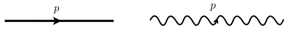
Figure 1: Propagators $G_{\varphi\varphi}(p)$ (left) and $G_{\chi\chi}(p)$ (right).

The propagator $G_{\varphi\omega}$ is also present in the theory. It has the the same $1/p^{2}$ momentum dependence as $G_{\chi_{i}\chi_{j}}$ but we will not need it in the examples below.

We may now turn on interaction $V(\phi)=\frac{\lambda}{4!}\phi^{4}$ or $\frac{g}{6}\phi^{3}$ for which $d_{uc}=6$ or $8$ respectively. Then we introduce bare and renormalized quantities (fields and coupling), and relate them by renormalization constants. These contants are obtained by requiring that correlators of renormalized quantities are finite as $\epsilon\to 0$.

We are interested in the $n\to 0$ limit of the theory. Note that the $n\to 0$ limit theory contains infinitely many fields $\chi_{2},\chi_{3},\chi_{4},\ldots$ which can appear on the external legs. To take the $n\to 0$ limit of any Feynman diagram we have to simplify the product of matrices $K_{ij}$ from the $\chi$ propagators, using $\Pi_{ij}\Pi_{jk}=(n-1)\Pi_{ik}\to-\Pi_{ik}$.

Consider first the $\phi^{4}$ case in $d=6-\epsilon$. The one-loop beta function $\beta_{\lambda}$ is computed from the coupling renormalization constant that can be obtained from a 4-point correlator e.g. $\langle\chi_{i}(p_{1})\chi_{j}(p_{2})\varphi(p_{3})\varphi(p_{4})\rangle$. Setting it to zero we get a fixed point at $\lambda_{\star}=\frac{64\pi^{3}\epsilon}{3}$. We do not show the computations as the steps are very similar to the $d=4-\epsilon$ usual $\phi^{4}$ (Wilson-Fisher) theory (see e.g. Kleinert and Schulte-Frohlinde (2001)).

The field renormalizations are obtained from 2-point functions, e.g. from the 2-loop correction to $\langle\chi_{i}(p)\chi_{j}(-p)\rangle$ one obtains the leading correction $\gamma_{\chi}$ to the dimension of $\chi_{i}$. We point out that due to the equivalence of (61) as $n\to 0$ with the SUSY theory the anomalous dimensions of all fundamental fields are equal, i.e. $\gamma_{\varphi}=\gamma_{\omega}=\gamma_{\chi}=\frac{\epsilon^{2}}{108}$. Note that this is the same field anomalous dimension as the usual Wilson-Fisher value, as expected from dimensional reduction. These computations are also very similar to $d=4-\epsilon$ so we do not show them.

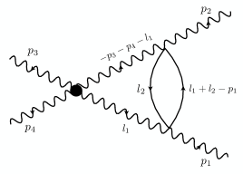
(a) $V(\phi)=\frac{\lambda}{4!}\phi^{4}$,

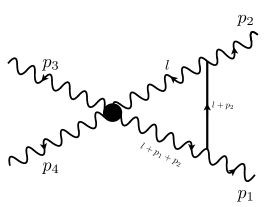
(b) $V(\phi)=\frac{g}{6}\phi^{3}$.

Figure 2: Computing the anomalous dimension of $(\mathcal{N}_{4})_{L}$ in the two theories.

Once we unerstand the RG flow of the basic Lagrangian (61) we start perturbing it by other leader interactions. The couplings of those interactions are kept infinitesimal, as we are just interested to know their scaling dimension. In other words, we are computing anomalous dimensions of various local operators of the theory, We do it in the standard way by defining the renormalization constant $Z_{\mathcal{O}}$ via $({\mathcal{O}})^{B}=Z_{{\mathcal{O}}}{\mathcal{O}}$ where $({\mathcal{O}})^{B}$ is a bare operator and ${\mathcal{O}}$ a renormalized operator. Then we have the anomalous dimension $\gamma_{{\mathcal{O}}}=\big{[}\frac{\partial}{\partial(\log\mu)}Z_{{\mathcal{O}}}\big{]}_{\lambda=\lambda_{\star}}$.

Let us demonstrate the computation with the example of $(\mathcal{N}_{4})_{L}=(\chi_{i}^{2})^{2}$ which is the SN leader with the lowest classical dimension. We use the correlation function $\langle(\mathcal{N}_{4})_{L}(p=0)\chi_{i}(p_{1})\chi_{j}(p_{2})\chi_{k}(p_{3})\chi_{l}(p_{4})\rangle$ and remove its $\epsilon\to 0$ singularities to compute $Z_{(\mathcal{N}_{4})_{L}}$. We choose this operator since its leading correction comes from a nontrivial 2-loop diagram shown in Fig. 2(a).

The evaluation of this 2-loop integral is not uncommon in the $\phi^{4}$ literature Kleinert and Schulte-Frohlinde (2001). The result is:

$$\frac{H^{2}\lambda^{2}}{(2\pi)^{2d}}\int\frac{d^{d}l_{1}d^{d}l_{2}}{l_{1}^{2}(l_{2}^{2})^{2}(l_{1}+p_{3}+p_{4})^{2}((l_{1}+l_{2}-p_{1})^{2})^{2}}=\frac{H^{2}\lambda^{2}}{2(4\pi)^{6}\epsilon}+O\left(\epsilon^{0}\right).$$ (63)

Requiring that the $\epsilon^{-1}$ divergence cancels (and taking into account the fundamental field renormalizations) we get:

$$Z_{(\mathcal{N}_{4})_{L}}^{-1}=1-\frac{4}{3}\frac{H^{2}\lambda^{2}}{(4\pi)^{6}\epsilon}\implies\gamma_{(\mathcal{N}_{4})_{L}}=-\frac{8}{27}\epsilon^{2}.$$ (64)

All other operators presented in the main text that have a 2-loop leading anomalous dimension involve the same loop integral. For the ones with a 1-loop leading correction the computation is similar to that of the beta function. The computations of beta function, field renormalization and anomalous dimensions of all operators considered in our work are shown in detail in App. H of Kaviraj et al. (2021).

For the $V(\phi)=\frac{g}{6}\phi^{3}$ potential in $d=8-\epsilon$ we define the bare quantities and renormalization constants in a similar way. The beta function and field renormalization constants are obtained from e.g. the correlators $\langle\chi_{i}(p_{1})\chi_{j}(p_{2})\varphi(p_{3})\rangle$ and $\langle\chi_{i}(p_{1})\chi_{j}(p_{2})\rangle$ respectively. We get a fixed point at $g_{\star}^{2}=-\frac{2}{3}\frac{(4\pi)^{4}\epsilon}{H}$ . The field anomalous dimensions are $\gamma_{\varphi}=\gamma_{\omega}=\gamma_{\chi}=-\frac{\epsilon}{18}$. As expected these are same as the usual $\phi^{3}$ theory in $d=6-\epsilon$ and the computations are also exactly similar (see e.g. Srednicki (2007) for the usual $\phi^{3}$ theory literature).

We may once again focus on the operator $(\mathcal{N}_{4})_{L}$ and compute its anomalous dimension. In this case the leading correction comes from the diagram as shown in Fig. 2(b). The loop integral is similar to that of the beta function and computed using standard techniques of the usual $\phi^{3}$ theory. It gives

$$\gamma_{(\mathcal{N}_{4})_{L}}=\frac{10}{9}\epsilon\,.$$ (65)

All other operators presented in the main text involve the same 1-loop integral. Details of all these computations will be given in a dedicated paper Kaviraj and Trevisani (2022).

References

- Parisi and Sourlas (1979) G. Parisi and N. Sourlas, Phys. Rev. Lett. 43, 744 (1979).
- Parisi and Sourlas (1981) G. Parisi and N. Sourlas, Phys. Rev. Lett. 46, 871 (1981).
- Aharony et al. (1976) A. Aharony, Y. Imry, and S. K. Ma, Phys. Rev. Lett. 37, 1364 (1976).
- Lubensky and Isaacson (1979) T. C. Lubensky and J. Isaacson, Phys. Rev. A 20, 2130 (1979).
- Redner (1979) S. Redner, J. Phys. A 12, L239 (1979).
- Gaunt (1980) D. S. Gaunt, J. Phys. A 13, L97 (1980).
- Hsu et al. (2005) H.-P. Hsu, W. Nadler, and P. Grassberger, J. of Phys. A 38, 775 (2005), arXiv:cond-mat/0408061 [cond-mat.stat-mech] .
- Fytas and Martín-Mayor (2013) N. G. Fytas and V. Martín-Mayor, Phys. Rev. Lett. 110, 227201 (2013), arXiv:1304.0318 [cond-mat.dis-nn] .
- Fytas et al. (2016) N. G. Fytas, V. Martin-Mayor, M. Picco, and N. Sourlas, Phys. Rev. Lett. 116, 227201 (2016), arXiv:1605.05072 [cond-mat.dis-nn] .
- Fytas et al. (2017) N. G. Fytas, V. Martin-Mayor, M. Picco, and N. Sourlas, Phys. Rev. E 95, 042117 (2017), arXiv:1612.06156 [cond-mat.dis-nn] .
- Fytas et al. (2019) N. G. Fytas, V. Martin-Mayor, G. Parisi, M. Picco, and N. Sourlas, Phys. Rev. Lett. 122, 240603 (2019), arXiv:1901.08473 [cond-mat.stat-mech] .
- Brézin and De Dominicis (1998) E. Brézin and C. De Dominicis, Europhys. Lett. 44, 13 (1998), cond-mat/9804266 .
- Feldman (2002) D. E. Feldman, Phys. Rev. Lett. 88, 177202 (2002), arXiv:cond-mat/0010012 [cond-mat.dis-nn] .
- Note (1) We stress that such a SUSY-breaking is explicit and not spontaneous.
- Note (2) Other theoretical ideas and methods used for understanding the phase transition in the RF models and the loss of PS SUSY include: formation of bound state of replicas Brézin and De Dominicis (2001); Parisi and Sourlas (2002), expansion at high temperature Gofman et al. (1996) and around the Bethe lattice Angelini et al. (2020), and the conformal bootstrap Hikami (2018, 2019). Comparison to functional renormalization group studies will be given at the end.
- Fisher (1978) M. Fisher, Phys. Rev. Lett. 40, 1610 (1978).
- Note (3) A special model of BP with microscopically realized SUSY Brydges and Imbrie (2003) was proven to undergo dimensional reduction in any . This result does not apply to generic (non SUSY) BP models or to the RF itself and does not shed light on why PS conjecture works for those models.
- Cardy (1983) J. L. Cardy, Physics Letters B 125, 470 (1983).
- Klein and Perez (1983) A. Klein and J. F. Perez, Physics Letters B 125, 473 (1983).
- Klein et al. (1984) A. Klein, L. J. Landau, and J. F. Perez, Commun. Math. Phys. 94, 459 (1984).
- Zaboronski (2002) O. V. Zaboronski, J. of Phys. A 35, 5511 (2002), arXiv:hep-th/9611157 [hep-th] .
- Kaviraj et al. (2020) A. Kaviraj, S. Rychkov, and E. Trevisani, JHEP 04, 090 (2020), arXiv:1912.01617 [hep-th] .
- Cardy (1985) J. L. Cardy, Physica D: Nonlinear Phenomena 15, 123 (1985).
- Note (4) This is clear e.g. from their propagator mixing different powers of momentum, see Cardy (1996), Eq. (8.39).
- Note (5) We note in this respect that replica symmetry breaking is proven not to happen in the RFIM Chatterjee (2015).
- Bray and Moore (1985) A. J. Bray and M. A. Moore, J. of Phys. C 18, L927 (1985).
- Fisher (1986) D. S. Fisher, Phys. Rev. Lett. 56, 416 (1986).
- Wilson and Kogut (1974) K. Wilson and J. B. Kogut, Phys.Rept. 12, 75 (1974).
- Kleinert and Schulte-Frohlinde (2001) H. Kleinert and V. Schulte-Frohlinde, Critical properties of theories (World Scientiic, 2001).
- Note (6) Here for simplicity we ignore interaction mixing effects, taken into account in the computations described below.
- Kaviraj et al. (2021) A. Kaviraj, S. Rychkov, and E. Trevisani, JHEP 03, 219 (2021), arXiv:2009.10087 [cond-mat.stat-mech] .
- Kupiainen and Niemi (1983) A. Kupiainen and A. Niemi, Physics Letters B 130, 380 (1983).
- (33) See appendices for more clarification on PS SUSY, dimensional reduction, properties of leader operators, leader families, and RG computations .
- Note (7) This is also supported by perturbative Parisi and Sourlas (1979); Kaviraj et al. (2021); Kaviraj and Trevisani (2022) and rigorous Lagrangian arguments Klein and Perez (1983); Klein et al. (1984).
- Wilson and Fisher (1972) K. G. Wilson and M. E. Fisher, Phys.Rev.Lett. 28, 240 (1972).
- Note (8) This was first conjectured in Kaviraj et al. (2021) and now we have a rigorous proof app .
- Note (9) The SW leader perturbation originating from the superstresstensor, , deserves a special comment. Naively it has dimension and is marginal. However, it is more properly classified as redundant. Its only effect is to rescale factor in (4\@@italiccorr), which is also a parameter entering the superspace metric. This rescaling can be undone by field redefinition and has no physical consequences.
- Kaviraj and Trevisani (2022) A. Kaviraj and E. Trevisani, (2022), arXiv:2203.12629 [hep-th] .
- Kehrein and Wegner (1994) S. K. Kehrein and F. Wegner, Nucl.Phys. B424, 521 (1994), arXiv:hep-th/9405123 [hep-th] .
- Note (10) For and odd we have , while has a SN leader.
- Note (11) Loop corrections grow rapidly with the number of fields inside the operator, making naive extrapolation to questionable. See Badel et al. (2019) for related recent work.
- Note (12) Actually none of the infinitely many discussed leaders become relevant for the case.
- Note (13) If relevant, this operator would break SUSY since it breaks superrotations.
- Note (14) Feldman Feldman (2002) argued that SUSY will be lost arbitrarily close to , because the negative anomalous dimension of interactions , , grows with making them to cross marginality closer and closer to as . We disagree with this argument as it does not take into account nonperturbative mixing Kaviraj et al. (2021). Our new results for the family strengthen this objection. The second respecting operator of this family, , stays irrelevant due to its positive one-loop dimension (see (21\@@italiccorr)). Nonperturbatively (while not in perturbation theory) is expected to mix with Feldman operators, and level crossing will be avoided. Hence, we expect that will provide a barrier which , , cannot cross, remaining irrelevant and unimportant for deciding the fate of SUSY.
- Guida and Zinn-Justin (1998) R. Guida and J. Zinn-Justin, J. Phys. A 31, 8103 (1998), arXiv:cond-mat/9803240 .
- Kompaniets and Panzer (2017) M. V. Kompaniets and E. Panzer, Phys. Rev. D 96, 036016 (2017), arXiv:1705.06483 [hep-th] .
- Kompaniets and Wiese (2020) M. Kompaniets and K. J. Wiese, Phys. Rev. E 101, 012104 (2020), arXiv:1908.07502 [cond-mat.stat-mech] .
- Tissier and Tarjus (2012) M. Tissier and G. Tarjus, Phys. Rev. B 85, 104203 (2012), arXiv:1110.5500 .
- Balog et al. (2020) I. Balog, G. Tarjus, and M. Tissier, Phys. Rev. E 102, 062154 (2020), arXiv:2008.13650 [cond-mat.dis-nn] .
- Note (15) But not for , because in this dimension the SUSY fixed point ceases to exist, see Kaviraj et al. (2021), Section 3.1.
- Brézin and De Dominicis (2001) E. Brézin and C. De Dominicis, Eur. Phys. J. B 19, 467 (2001), cond-mat/0007457 .
- Parisi and Sourlas (2002) G. Parisi and N. Sourlas, Phys. Rev. Lett. 89, 257204 (2002), arXiv:cond-mat/0207415 .
- Gofman et al. (1996) M. Gofman, J. Adler, A. Aharony, A. B. Harris, and M. Schwartz, Phys. Rev. B 53, 6362 (1996).
- Angelini et al. (2020) M. C. Angelini, C. Lucibello, G. Parisi, F. Ricci-Tersenghi, and T. Rizzo, Proc. Nat. Acad. Sci. 117, 2268 (2020), arXiv:1906.04437 [cond-mat.dis-nn] .
- Hikami (2018) S. Hikami, PTEP 2018, 123I01 (2018), arXiv:1708.03072 [hep-th] .
- Hikami (2019) S. Hikami, PTEP 2019, 083A03 (2019), arXiv:1801.09052 [cond-mat.dis-nn] .
- Brydges and Imbrie (2003) D. C. Brydges and J. Z. Imbrie, Ann. Math. 158, 1019 (2003), arXiv:math-ph/0107005 .
- Cardy (1996) J. L. Cardy, Scaling and renormalization in statistical physics (Cambridge, UK: Univ. Pr., 238 p., 1996).
- Chatterjee (2015) S. Chatterjee, Comm. Math. Phys. 337, 93 (2015), arXiv:1404.7178 [math-ph] .
- Badel et al. (2019) G. Badel, G. Cuomo, A. Monin, and R. Rattazzi, JHEP 11, 110 (2019), arXiv:1909.01269 [hep-th] .
- Nakayama (2015) Y. Nakayama, Phys. Rept. 569, 1 (2015), arXiv:1302.0884 [hep-th] .
- Srednicki (2007) M. Srednicki, Quantum Field Theory (Cambridge University Press, 2007).