Diffractive longitudinal structure function at the Electron Ion Collider

Abstract

Possibilities for the measurement of the longitudinal structure function in diffraction $F_{\mathrm{L}}^{\mathrm{D}}$ at the future US Electron Ion Collider are investigated. The sensitivity to $F_{\mathrm{L}}^{\mathrm{D}}$ arises from the variation of the reduced diffractive cross section with centre-of-mass energy. Simulations are performed with various sets of beam energy combinations and for different assumptions on the precision of the diffractive cross section measurements. Scenarios compatible with current EIC performance expectations lead to an unprecedented precision on $F_{\mathrm{L}}^{\mathrm{D}}$ at the 5-10% level in the best measured regions. While scenarios with data at a larger number of centre-of-mass energies allow the extraction of $F_{\mathrm{L}}^{\mathrm{D}}$ in the widest kinematic domain and with the smallest uncertainties, even the more conservative assumptions lead to precise measurements. The ratio $R^{\mathrm{D}}$ of photoabsorption cross sections for longitudinally to transversely polarised photons can also be obtained with high precision using a separate extraction method.

1 Introduction

Diffraction in deep inelastic scattering (DIS) was studied extensively at the Hadron-Elektron-Ringanlage (HERA) collider at DESY. The measurements showed that it gives a large contribution, of about $\sim 10$%, to the total cross section  [1, 2], see the review [3] and refs. therein. Diffractive events are characterised by the measurement of either a proton (in the case of coherent diffraction) or a state with the proton quantum numbers (incoherent diffraction). Experimentally, diffractive events are defined either by the identification of a proton in dedicated far-forward detectors housed in Roman pot insertions to the beampipe (see for example [4, 5, 6, 7]), or by a lack of hadronic activity in a sizeable kinematic region adjacent to the outgoing proton beam, i.e. the presence of a large rapidity gap (LRG) (see for example [7, 8, 9]). Based on the experimental results from HERA, it was possible to analyse the partonic structure of the $t$-channel colourless exchange in such events. A successful description of the diffractive structure functions was achieved at high $Q^{2}$ based on the collinear factorization and Dokshitzer-Gribov-Lipatov-Altarelli-Parisi (DGLAP) evolution of the corresponding diffractive parton densities (DPDF) [4, 10]. The latter quantities parametrize the partonic content of the colourless exchange in the diffractive events.

Diffraction has been a central subject in investigations of strong interactions for many decades [11, 12]. As a pure quantum phenomenon, some properties derive from basic requirements like unitarity. On the other hand, the microscopic dynamics by which a composite object, a hadron or nucleus, is able to undergo a high energy collision and remain colourless with its constituents bound, is closely related to the confinement mechanism [13]. Besides, diffraction is very sensitive to the high energy behaviour of Quantum Chromodynamics (QCD), specifically to the low-$x$ distribution of partons and its energy evolution [14]. Therefore, it is a promising observable for observing deviations from linear evolution like higher twist effects or parton saturation. Diffractive $ep$ scattering is also related to nuclear shadowing on deuterons [15] and tests the validity of perturbative factorisation [16, 17, 18] – known to be violated in diffractive dijet photoproduction [19]. Furthermore, due to the simplicity of the final state, diffractive events may offer new opportunities for the detection of rare phenomena, see [20] and refs. therein.

Among the various diffractive observables that can be measured in DIS, a very interesting one, yet experimentally challenging, is the diffractive longitudinal structure function $F_{\mathrm{L}}^{\mathrm{D}}$. Given by the coupling of virtual photons with longitudinal polarisation to the hadron that undergoes the diffractive interaction, it is – as in the case of inclusive events – a more sensitive probe of the gluon content of the target and of the QCD evolution than the diffractive structure function $F_{\mathrm{2}}^{\mathrm{D}}$, which is only sensitive to the gluon content via evolution. $F_{\mathrm{L}}^{\mathrm{D}}$ also probes contributions from higher twists, similarly to the inclusive case, see [21]. Thus, its measurement gives the opportunity of constraining the gluon contribution to diffraction in DIS and the dynamics beyond linear evolution driving this kind of interaction.

$F_{\mathrm{L}}^{\mathrm{D}}$ is a very poorly known quantity, with the only existing experimental study done by the H1 Collaboration [22] at HERA. On top of the intrinsic difficulty of disentangling diffractive from inclusive events, measuring the longitudinal structure function requires variation of the centre-of-mass energy of the lepton-hadron collisions. At HERA the former was determined by the LRG method. For the latter, four energies of the proton beam were employed, additionally selecting those events with high inelasticity of the electron (see below) where the contribution of the longitudinal structure function to the total reduced cross section is largest. This region is difficult experimentally, since it is associated with low electron energies and with the hadronic final state being produced in the same backward pseudorapidity region as the scattered electron.

Planned DIS colliders like the Electron Ion Collider (EIC) [23, 24], the Large Hadron-electron Collider (LHeC) [25, 26] or the Future-Circular-Collider in its electron-hadron option (FCC-eh) [27, 28] will benefit from larger integrated luminosities exceeding those at HERA by factors ${\cal O}(1000)$ and new detector techniques providing enhanced possibilities for separating diffractive from non-diffractive events.

In previous works we analysed the potential of the measurements of the diffractive reduced cross section at the LHeC and FCC-he and at the EIC [29, 30] as well as the possibility for constraining the diffractive parton distribution functions. In this work we focus on the possibilities for the determination of $F_{\mathrm{L}}^{\mathrm{D}}$ in coherent diffraction on protons at the EIC, where simulations of the forward detectors, including their effect on particle reconstruction, are available [24].

The manuscript is organised as follows. In Sec. 2 we present the general expressions and kinematics that will be used in our analysis and discuss the experimental aspects of proton tagging at the EIC. In Sec. 3 we discuss the generation of simulated EIC data (‘pseudodata’) and the method of extraction of $F_{\mathrm{L}}^{\mathrm{D}}$ as well as the choices of beam energies. Results are presented in Sec. 4, first for the reduced cross section $\sigma_{\mathrm{red}}^{\mathrm{D(3)}}$ and then for $F_{\mathrm{L}}^{\mathrm{D(3)}}$. We then proceed to discuss the influence of the systematic error assumed in the pseudodata and the assumptions on the beam configurations. Results for $R^{\mathrm{D(3)}}=F_{\mathrm{L}}^{\mathrm{D(3)}}/F_{\mathrm{T}}^{\mathrm{D(3)}}$ are also presented. We end with conclusions in Sec. 5.

2 Definitions and kinematics

2.1 Diffractive variables and definitions

In this work we focus on neutral current diffractive deep inelastic scattering (DDIS) in the one photon exchange approximation, neglecting radiative corrections whose contribution can be corrected. For an electron or positron with four momentum $l$ and a proton with four-momentum $P$, the diagram is shown in Fig. 1. A characteristic feature of the diffractive process, as illustrated in Fig. 1, is the presence of the rapidity gap between the final proton (or its dissociated state) $Y$ and the system $X$. It is mediated by the colourless object, indicated by $P/R$, to which we refer generally as ‘diffractive exchange’.

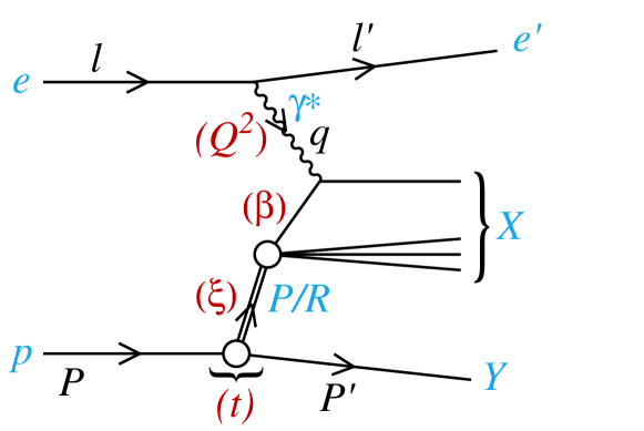
Figure 1: Diagram showing the neutral current diffractive DIS process and the relevant kinematic variables in the one photon exchange approximation.

In DDIS several variables can be defined in terms of the four-momenta indicated in Fig. 1 and the usual Mandelstam variables:

$$Q^{2} = -q^{2}\ ,$$

$$y = \frac{P\cdot q}{P\cdot\ell}\ ,$$

$$x = \frac{Q^{2}}{2P\cdot q}=\frac{Q^{2}}{ys}\ ,$$

$$\beta = \frac{Q^{2}}{2\,(P-P^{\prime})\cdot q}\ ,$$

$$\xi = \frac{x}{\beta}\ ,$$

$$t = (P^{\prime}-P)^{2}\ .$$ (1)

Besides the standard DIS variables $s,Q^{2},y,x$, in DDIS some additional variables appear: $t$ is the squared four-momentum transfer at the proton vertex, $\xi$ (alternatively denoted by $x_{I\!\!P}$) can be interpreted as the momentum fraction of the ‘diffractive exchange’ with respect to the beam hadron, and $\beta$ is the momentum fraction of the parton (probed by the virtual photon) with respect to the diffractive exchange. In Fig. 2 we show the kinematic coverage in $x$ and $Q^{2}$ of the EIC for three selected energies compared to that of HERA. Since HERA was operating at higher centre-of-mass energy than the EIC, it could reach lower values of $x$. The EIC can operate at several energy combinations, which will result in a wide coverage of $x$ also towards moderate and large $x$, and which is essential for $F_{\mathrm{L}}^{\mathrm{D}}$ measurement. In Fig. 2 only three beam energy combinations are shown, a subset of a wider range of combinations possible at the EIC, see the discussion below.

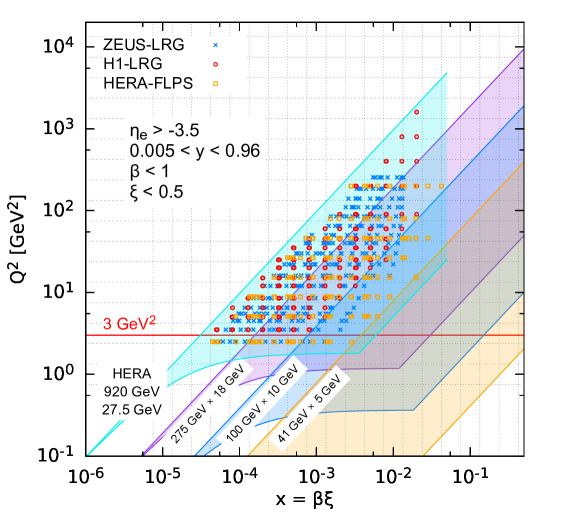
Figure 2: Kinematic $x-Q^{2}$ plane showing different choices of beam energies at the EIC and the region covered by HERA experiments. Note that $\eta_{e}>-3.5$ corresponds to an angular acceptance of 176.5 degrees for the electron.

Only four variables, usually chosen to be $\beta,\xi,Q^{2},t$, are needed to characterise the reduced cross section, related to the measured cross section by

$$\frac{d^{4}\sigma^{\mathrm{D}}}{d\xi d\beta dQ^{2}dt}=\frac{2\pi\alpha_{\rm em}^{2}}{\beta Q^{4}}\,Y_{+}\,\sigma_{\mathrm{red}}^{\mathrm{D}(4)}\,,$$ (2)

where $Y_{+}=1+(1-y)^{2}$. It is also customary to perform an integration over $t$, defining

$$\frac{d^{3}\sigma^{\mathrm{D}}}{d\xi d\beta dQ^{2}}=\frac{2\pi\alpha_{\rm em}^{2}}{\beta Q^{4}}\,Y_{+}\,\sigma_{\mathrm{red}}^{\mathrm{D}(3)}\,.$$ (3)

In the one photon exchange approximation, the reduced cross sections can be expressed in terms of two diffractive structure functions $F_{2}^{\mathrm{D}}$ and $F_{\mathrm{L}}^{\mathrm{D}}$:

$$\sigma_{\mathrm{red}}^{\mathrm{D}(4)}=F_{2}^{\mathrm{D}(4)}(\beta,\xi,Q^{2},t)-\frac{y^{2}}{Y_{+}}F_{\mathrm{L}}^{\mathrm{D}(4)}(\beta,\xi,Q^{2},t)\;,$$ (4)

$$\sigma_{\mathrm{red}}^{\mathrm{D}(3)}=F_{2}^{\mathrm{D}(3)}(\beta,\xi,Q^{2})-\frac{y^{2}}{Y_{+}}F_{\mathrm{L}}^{\mathrm{D}(3)}(\beta,\xi,Q^{2})\;,$$ (5)

where $F_{\mathrm{2,L}}^{\mathrm{D}(4)}$ have dimension $\mathrm{GeV}^{-2}$ and $F_{\mathrm{2,L}}^{\mathrm{D}(3)}$ are dimensionless.

The dependence of the reduced cross sections $\sigma_{\mathrm{red}}^{\mathrm{D}(4,3)}$ on the centre-of-mass energy comes via the inelasticity $y=\frac{Q^{2}}{\xi\beta s}$. Due to the $Y_{+}$ factor, $\sigma_{\mathrm{red}}^{\mathrm{D}(4,3)}\simeq F_{2}^{\mathrm{D}(4,3)}$ when $y$ is not too close to unity.

Both reduced cross sections $\sigma_{\mathrm{red}}^{\mathrm{D}(3)}$ and $\sigma_{\mathrm{red}}^{\mathrm{D}(4)}$ have been measured at HERA [1, 2, 31, 4, 32, 33, 10, 5, 34]. These data have been used for perturbative QCD analyses based on collinear factorization [16, 17, 18], where the diffractive cross section reads

$$d\sigma^{ep\rightarrow eXY}(\beta,\xi,Q^{2},t)\;=\;\sum_{i}\int_{\beta}^{1}dz\ d\hat{\sigma}^{ei}\left(\frac{\beta}{z},Q^{2}\right)\,f_{i}^{\rm D}(z,\xi,Q^{2},t)\;,$$ (6)

up to terms of order ${\cal O}(1/Q^{2})$. Here, the sum is performed over all parton species (gluon and all quark flavours). The hard scattering partonic cross section $d\hat{\sigma}^{ei}$ can be computed perturbatively in QCD and is the same as in the inclusive deep inelastic scattering case. The long distance part $f_{i}^{\rm D}$ corresponds to the DPDFs, which can be interpreted as conditional probabilities for partons in the proton, provided the proton is scattered into the final state system $Y$ with four-momentum $P^{\prime}$. They are non-perturbative objects to be extracted from data, but their evolution through the DGLAP evolution equations [35, 36, 37, 38] can be computed perturbatively, similarly to the inclusive case. The analogous formula for the $t$-integrated structure functions reads

$$F_{2/\mathrm{L}}^{\mathrm{D}(3)}(\beta,\xi,Q^{2})=\sum_{i}\int_{\beta}^{1}\frac{dz}{z}\,C_{2/\mathrm{L},i}\Big{(}\frac{\beta}{z}\Big{)}\,f_{i}^{\mathrm{D}(3)}(z,\xi,Q^{2})\;,$$ (7)

where the coefficient functions $C_{2/\mathrm{L},i}$ are the same as in inclusive DIS and the DPDFs $f_{i}^{\mathrm{D}(3)}(z,\xi,Q^{2})$ have been determined from comparisons to HERA data [1, 2, 31, 4, 32, 33, 10, 5, 34].

2.2 Experimental Considerations

As can be inferred from Eq. 5, sensitivity to $F_{\mathrm{L}}^{\mathrm{D}}$ is strongest as $y\rightarrow 1$. Experimentally, this is a region in which backgrounds are hard to control, since it corresponds to the lowest scattered electron energies and also to cases where hadronic final state particles are produced in the same (backward) pseudorapidity region as the scattered electron. Extractions of the inclusive and diffractive longitudinal structure functions therefore place strong challenges on the performance of electromagnetic calorimetry, tracking and particle identification in the backward region of the detector. H1 achieved measurements down to electron energies of around 3 GeV. At the EIC, where charged pion rejection factors relative to electrons of the order of $10^{-4}$ are targeted, the aim is to go substantially lower, even into the sub-GeV range. Here, we apply an upper $y$ cut of 0.96, which is typical of current EIC studies. The targeted $\eta$ range of the EIC experiments, with calorimeter and tracking coverage to at least as far backwards as $\eta=-3.5$, provides full coverage for scattered electrons with $Q^{2}>1$ GeV².

In the H1 measurement [22], the use of the LRG method of selecting diffractive events led to a normalisation uncertainty of 7%. This uncertainty can in principle be eliminated through the use of beamline proton tagging based on instrumentation housed in Roman pot insertions to the beampipe. In contrast to the situation at previous colliders, beamline instrumentation has been a fundamental consideration from the outset at the EIC. It is essential to the success of the diffractive programme, as illustrated in Fig. 3, where the rapidity ranges covered by the undecayed final state system $X$ and proton are shown as a function of $\xi$ for four combinations of electron and proton beam energies. The bands correspond to ranges $\beta\in[0.1,0.9]$ and $p_{\perp}$ of the final state proton below $4\,\mathrm{GeV}$. The decay of the $X$ system into a multi-particle hadronic system extends its extent forwards in pseudorapidity in a manner that scales logarithmically with $\xi$, reducing the size the rapidity gap. For comparison, gaps smaller than about 3 pseudorapidity units could not be used reliably at HERA due to the poorly modelled contributions from gaps produced from hadronisation fluctuations in non-diffractive processes. Whilst fairly large rapidity gaps exist at the lowest $\xi$ values and highest EIC centre-of-mass energies, it is clear that throughout most of the EIC phase space and for most of the expected beam configurations, LRG methods will yield poor performance.

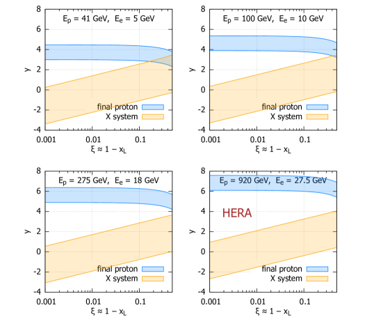
Figure 3: Ranges in the rapidity of the scattered proton and the undecayed dissociative system $X$ as a function of $\xi$ for three different beam energy combinations at the EIC and for HERA. The bands correspond to all cases where the proton transverse momentum is lower than 4 GeV, $0.005<y<0.96$ and $0.1<\beta<0.9$.

The most recent studies of the physics and detector requirements at the EIC envisage multiple beamline proton spectrometers, allowing a full determination of the outgoing proton kinematics with good measurements of both $\xi$ and $t$. In Fig. 4 we show the kinematic coverage for the forward proton considered in [24]. In contrast to the LRG method, the multiple planned detector stations with a combined angular acceptance $0.5-20$ mrad lead to a wide potential measurement range in $\xi$ and $t$ for all beam energies. Measurements up to $\xi$ values as large as 0.5 may be possible, well beyond the range in which diffractive ($t$-channel exchange) processes are expected to be the dominant mechanism for leading proton production. We therefore assume here that events will be selected based on the scattered proton and that the accessible phase space in $\xi$ is not strongly limited experimentally.

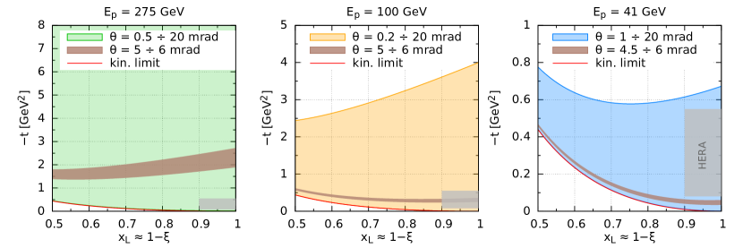
Figure 4: Final proton tagging. $x_{\mathrm{L}},t$ range of the proton tagged by the EIC detector for three proton energies, 275 GeV, 100 GeV and 41 GeV. The brown strip marks a small ($\sim$ 1 mrad) region not covered by the current detector design.

The standard Rosenbluth method of extracting longitudinal structure functions involves fits to data at the same $\xi$, $\beta$ and $Q^{2}$ values, but different centre-of-mass energies. Systematic uncertainties that are not correlated between different beam energies therefore tend to propagate into larger uncertainties on $F_{\mathrm{L}}^{\mathrm{D}}$ than those that are positively correlated between beam energies. Since statistical uncertainties are completely uncorrelated between different beam energies, $F_{\mathrm{L}}^{\mathrm{D}}$ measurements are also particularly sensitive to the available sample sizes.

Due to the relatively small integrated luminosities in the reduced proton beam energy runs, the HERA measurement of $F_{\mathrm{L}}^{\mathrm{D(3)}}$ [22] was limited by statistical uncertainties throughout most of the phase space. Since the integrated luminosity expected at the EIC is around three orders of magnitude larger than that at HERA, the sample sizes will be much larger (integrated luminosities of 10 fb^-1 per beam energy are assumed here) and statistical uncertainties are expected to be unimportant.

A detailed systematic uncertainty analysis was carried out in the HERA measurement, with the conclusion that no single source dominated, but also giving some baseline from which to extrapolate to the likely precision achievable on the cross sections at a future collider such as the EIC. The best precision achieved in diffractive reduced cross section measurements at HERA was at the 4% level, with uncorrelated sources contributing as little as 2%, arising primarily from track-cluster linking and vertex finding efficiencies. Recent and ongoing studies of proposed EIC instrumentation solutions [24] already indicate that uncertainties of this kind will be dramatically reduced at the EIC. We therefore consider scenarios in which the uncertainties that are uncorrelated between beam energies are either 1% or 2%. With sources related to the LRG method eliminated, correlated systematic uncertainties are also expected to be reduced significantly. The alignment and calibration procedures required in Roman pot methods inherently lead to correlated systematics, but using methods developed at HERA [39, 40, 41], coupled with the substantial further evolution of proton-tagging techniques at the LHC [42, 43, 44, 45] and future EIC-specific work, we estimate that these are controllable to the sub-2% level, and will thus have a negligible effect on the $F_{\mathrm{L}}^{\mathrm{D}}$ extraction compared with the uncorrelated sources.

3 Method

3.1 Pseudodata generation

We shall first describe the pseudodata generation for our simulations. The momentum transfer $t$ is integrated over in this analysis. Let us rewrite Eq. (5) as

$$\sigma_{\mathrm{red}}^{\mathrm{D}(3)}=F_{2}^{\mathrm{D}(3)}(\beta,\xi,Q^{2})-Y_{\mathrm{L}}\,F_{\mathrm{L}}^{\mathrm{D}(3)}(\beta,\xi,Q^{2})\;,$$ (8)

where

$$Y_{\mathrm{L}}=\frac{y^{2}}{Y_{+}}=\frac{y^{2}}{1+(1-y)^{2}}\;.$$ (9)

As mentioned previously, the extraction of the longitudinal diffractive structure function relies on the possibility of disentangling it from $F_{2}^{D}$, as is evident in the formula above for the reduced cross section. This is possible if, for fixed $(\beta,Q^{2},\xi)$, one can vary $Y_{\mathrm{L}}$, and hence $y$, in a sufficiently wide range. Given that $y=Q^{2}/(s\beta\xi)$ it is therefore necessary to perform measurements of the reduced cross section using different centre-of-mass energies. The EIC is uniquely positioned to perform such a measurement, thanks to its design, which allows for a wide range of different beam energies.

We have considered several beam energies for both the electrons and the protons, within the range expected for the EIC:

$$E_{e} =5,10,18\,\mathrm{GeV}\,,$$

$$E_{p} =41,100,120,165,180,275\,\mathrm{GeV}\,.$$ (10)

These beam energies combine to give 17 distinct centre-of-mass energies (there is a degeneracy in this choice since two combinations $10\times 180$ and $18\times 100$ lead to the same centre-of-mass energy, $85\,\mathrm{GeV}$). The centre-of-mass energies corresponding to all combinations are given in Table 1. In order to test the sensitivity of $F_{\mathrm{L}}^{\mathrm{D(3)}}$ to the available beam energies, we consider three different subsets in the analysis :

• 17 values — all combinations from Table 1 except for $10\times 180$.

• 9 values — marked bold in Table 1,

• 5 values — marked bold against a green background in Table 1.

Set S-17 contains the widest range of possibilities. S-5 is the set of combinations that has often been assumed in EIC studies to date [24]. Additionally, we consider an intermediate set S-9, which restricts the list to three proton and three electron beam energies, whilst maintaining the same overall kinematic range as S-17.

		$E_{p}\,[\mathrm{GeV}]$
		41	100	120	165	180	275
$E_{e}\,[\mathrm{GeV}]\;$	5	29	45	49	57	60	74
	10	40	63	69	81	85	105
	18	54	85	93	109	114	141

Table 1: Centre-of-mass energies (in GeV) for various combinations of beam energies.

The pseudodata for the reduced diffractive cross section at the EIC were generated using Eqs. (5) and (7). The diffractive parton distribution used for the evaluation of the cross section is the ZEUS-SJ set [46]. This fit uses inclusive diffractive data together with diffractive DIS dijet data, which are added to improve the constraints on the diffractive gluon distribution.

The details of the ZEUS-SJ parametrization closely follow those of [8] and can be found in [46]. Below we summarize a few important features. The diffractive parton densities are parametrized using a two-component form:

$$f_{i}^{\mathrm{D}(4)}(z,\xi,Q^{2},t)=f^{p}_{{I\!\!P}}(\xi,t)\,f_{i}^{{I\!\!P}}(z,Q^{2})+f^{p}_{{I\!\!R}}(\xi,t)\,f_{i}^{{I\!\!R}}(z,Q^{2})\;.$$ (11)

The first term in Eq. (11) is interpreted as the exchange of a ‘Pomeron’ and the second is a ‘Reggeon’ component. They dominate in different $\xi$ regions: the ‘Pomeron’ is dominant for $\xi\leq 0.01$. The ‘Reggeon’ starts to be important for $\xi>0.01$ and becomes dominant for $x>0.1$. For both terms, proton vertex factorization is assumed, which means that the diffractive parton density factorizes into a parton distribution in a diffractive exchange $f_{i}^{{I\!\!P},{I\!\!R}}$ and a flux factor $f^{p}_{{I\!\!P},{I\!\!R}}$. The parton distribution in the ‘Pomeron’ and ‘Reggeon’ $f_{i}^{{I\!\!P},{I\!\!R}}(\beta,Q^{2})$ only depend on the longitudinal momentum fraction $\beta$ of the parton with respect to the Pomeron/Reggeon and the photon virtuality $Q^{2}$. The flux factors $f^{p}_{{I\!\!P},{I\!\!R}}(\xi,t)$, on the other hand, only depend on $\xi$, which is related to the size of the rapidity gap, and the momentum transfer at the proton vertex $t$. They represent the probability that a Pomeron/Reggeon with given values of $\xi,t$ couples to the proton. The flux factors are parametrized using a form motivated by Regge theory:

$$f^{p}_{{I\!\!P},{I\!\!R}}(\xi,t)=A_{{I\!\!P},{I\!\!R}}\frac{e^{B_{{I\!\!P},{I\!\!R}}t}}{\xi^{2\alpha_{{I\!\!P},{I\!\!R}}(t)-1}}\,,$$ (12)

with a linear trajectory ${\alpha_{{I\!\!P},{I\!\!R}}(t)=\alpha_{{I\!\!P},{I\!\!R}}(0)+\alpha_{{I\!\!P},{I\!\!R}}^{\prime}\,t}$.

The diffractive parton distributions are evolved using the NLO DGLAP equations. For the case of the Pomeron at the initial scale $\mu_{0}^{2}=1.8\,\mathrm{GeV}^{2}$ they are parametrized as

$$zf_{i}^{I\!\!P}(z,\mu_{0}^{2})=A_{i}z^{B_{i}}(1-z)^{C_{i}}\;,$$ (13)

where $i$ is a gluon or a light quark. In the diffractive parametrizations all the light quarks (anti-quarks) are assumed to be equal. For the treatment of heavy flavours, a variable flavour number scheme (VFNS) is adopted, where the charm and bottom quark DPDFs are generated radiatively via DGLAP evolution. There is no intrinsic heavy quark distribution present. The structure functions are calculated in a General-Mass Variable Flavour Number scheme (GM-VFNS) [47, 48] which ensures a smooth transition of $F_{\mathrm{2,L}}$ across the flavour thresholds by including $\mathcal{O}(m_{h}^{2}/Q^{2})$ corrections.

The model that we use to compute the diffractive cross section is state of the art. Still, it contains substantial uncertainties in the Reggeon contribution, which was poorly constrained by HERA data. Whilst these uncertainties affect the predicted cross sections and structure functions, they do not to first order impact our assessment of the feasibility of measuring the longitudinal diffractive structure function, which is our primary objective here.

The parton distributions for the Reggeon component are taken from a parametrization which was obtained from fits to the pion structure function [49, 50]. HERA data required the addition of the Reggeon contribution, but could not constrain it. The high $\xi$ region where it dominates is accessible in the EIC kinematics, and the possibilities for disentangling the Reggeon contribution (or any contribution other than the Pomeron) were discussed in [24]. This is an aspect demanding a dedicated study that we leave for the future.

The pseudodata were generated as the extrapolation of the fit to HERA [46], amended with a random Gaussian smearing with standard deviation corresponding to the relative error $\delta$. The total error was assumed to be composed of systematic and statistical components and computed as

$$\delta=\sqrt{\delta^{2}_{\rm sys}+\delta^{2}_{\rm stat}}\,.$$ (14)

The statistical error was evaluated assuming an integrated luminosity $10\,{\rm fb}^{-1}$, see [24]. For the binning adopted in this study, the statistical uncertainties have a very small effect on the extraction of the longitudinal structure function. As discussed in Sec. 2.2, correlated systematic uncertainties on the reduced cross section are also expected to be relatively unimportant in the $F_{\mathrm{L}}^{\mathrm{D}}$ extraction and are thus neglected here. For the uncorrelated systematic error we have considered two scenarios, with $2\%$ and $1\%$ ascribed to each data point.

The cuts imposed for the data selection are:

• $Q^{2}\geq 3\;\mathrm{GeV}^{2}$ : both the H1 [32] and the ZEUS [46] analyses of the inclusive diffractive data observed that the quality of the DGLAP-based fit deteriorates in the low $Q^{2}$ region, possibly because it is sensitive to higher twist contributions. This cut is imposed to limit the sensitivity to such effects. The EIC kinematics and expected scattered electron coverage lead to full acceptance for all $x$ in the chosen $Q^{2}$ region at all beam energies, see Fig. 2.

• $y$ between 0.005 and 0.96, which is the expected coverage of a typical measurement whilst maintaining well-controlled systematics.

We adopt a uniform logarithmic binning with four bins per decade for each of $\xi,\beta$ and $Q^{2}$ . This results in the numbers of $\sigma_{\mathrm{red}}$ data points for each $(\xi,\beta,Q^{2})$ bin as shown in Fig. 5. Taking into account that we require four points for the linear fit (see Sec. 3.2) to extract $F_{\mathrm{L}}^{\mathrm{D(3)}}$, the analysis therefore proceeds with a total of 364 $F_{\mathrm{L}}^{\mathrm{D(3)}}$ values for set S-17, 285 $F_{\mathrm{L}}^{\mathrm{D(3)}}$ values for set S-9 and 160 $F_{\mathrm{L}}^{\mathrm{D(3)}}$ values for set S-5.

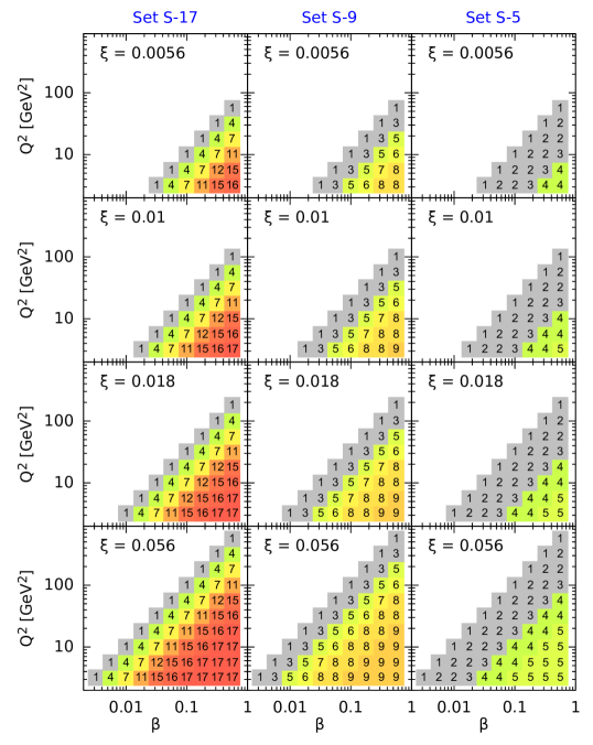
Figure 5: Count of different beam energy combinations from among set S-17 that lead to measurable $\sigma_{\mathrm{red}}^{\mathrm{D}(3)}$ data points for each $(\xi,\beta,Q^{2})$ bin. Only cases with a number of counts $\geq 4$ are considered for the extraction of $F_{\mathrm{L}}^{\mathrm{D(3)}}$.

3.2 Extraction of the diffractive longitudinal structure function

The extraction of the diffractive longitudinal structure function $F_{\mathrm{L}}^{\mathrm{D(3)}}$ is performed using the same method as in the H1 analysis [22]. This method was adapted from the measurements of the inclusive longitudinal structure function $F_{\mathrm{L}}$, see [52, 53, 54]. The reduced cross section is a linear function of $Y_{\mathrm{L}}$, see Eq. (8). The structure function $F_{\mathrm{L}}^{\mathrm{D(3)}}$ can thus be found by performing a linear fit, and extracting the slope of $\sigma_{\mathrm{red}}^{\mathrm{D}(3)}$ as a function of $Y_{\mathrm{L}}$. This is done for every set of values in $Q^{2}$, $\xi$ and $\beta$ for which there are four or more available $\sigma_{\mathrm{red}}$ values (in the H1 analysis [22] only three points were required). In Figs. 6 and 7 examples of fits in 4 bins of $(\xi,\beta,Q^{2})$ are shown, which are discussed in detail in Subsec. 4.1.

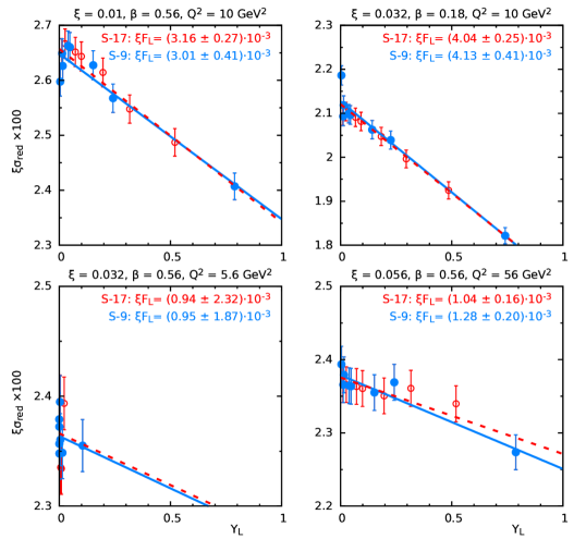
Figure 6: Examples of the $\sigma_{\mathrm{red}}^{\mathrm{D}(3)}=F_{2}^{\mathrm{D(3)}}-Y_{\mathrm{L}}F_{\mathrm{L}}^{\mathrm{D(3)}}$ fit. Comparison between set S-17 (red line and points) and S-9 (blue line and points).

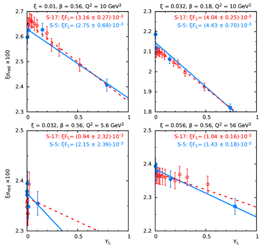
Figure 7: Examples of the $\sigma_{\mathrm{red}}^{\mathrm{D}(3)}=F_{2}^{\mathrm{D(3)}}-Y_{\mathrm{L}}F_{\mathrm{L}}^{\mathrm{D(3)}}$ fit. Comparison between set S-17 (red line and points) and S-5 (blue line and points).

4 Results

In this Section we show the simulated results for $F_{\mathrm{L}}^{\mathrm{D(3)}}$ and analyse the influence of choices of beam energies, systematic errors and numbers of measurements. We also extract results for $R=F_{\mathrm{L}}^{\mathrm{D(3)}}/F_{\mathrm{T}}^{\mathrm{D(3)}}$. In obtaining uncertainties on $F_{\mathrm{L}}^{\mathrm{D(3)}}$ from fits to Eq. 8, we take 68% confidence limits (CL). This practically corresponds to $1\sigma$ errors for a number of degrees of freedom $\mathrm{NDF}\gtrsim 10$. However, many $(\xi,Q^{2},\beta)$ bins where $F_{\mathrm{L}}^{\mathrm{D(3)}}$ is fitted contain even as few data points as 4, which results in 68% CL error equal to $\simeq 1.3\,\sigma$.

4.1 Influence of systematic errors and choices of beam energies

In Figs. 6 and 7 examples of fits are shown in 4 selected bins of $(\xi,\beta,Q^{2})$. In each figure two data sets are shown. The open red circles correspond to set S-17, and the filled blue points are the subset that is also present in S-9 (for Fig. 6) and S-5 (for Fig. 7). Uncorrelated systematic uncertainties are considered at the level of $1\%$ on each data point, with the influence of correlated sources taken to be negligible as discussed previously. Separate fits are performed to each of the sets, resulting in the two lines shown on each of the plots.

The S-17 set of beam energies contains the most points in $Y_{\mathrm{L}}$ and therefore by construction gives the most precise results. Reducing the number of beam energy combinations lowers the precision of the $F_{\mathrm{L}}^{\mathrm{D(3)}}$ extraction. However, we observe that the fits with S-9 and even S-5 do not deviate strongly from those of S-17 in most cases. This is encouraging, since set S-5 is the current working hypothesis for the EIC energy combinations. It is also evident that the strongest variations with the choice of set arise in $(Q^{2},\xi,\beta)$ bins where there is a limited range of $Y_{\mathrm{L}}$ available for the fit. For example, the bin with $(\xi=0.032,\beta=0.56,Q^{2}=5.6\,\mathrm{GeV}^{2})$ has a very small range in $Y_{\mathrm{L}}$, resulting in large variations between the sets and correspondingly large uncertainties on the extracted $F_{\mathrm{L}}^{\mathrm{D(3)}}$, despite the relatively large number of $Y_{L}$ points. The relative accuracy of the $F_{\mathrm{L}}^{\mathrm{D(3)}}$ extraction also depends on its absolute size, which is reflected in the steepness of the slope.

For each choice of beam energy combinations and systematic precision, ten Monte Carlo simulations are carried out in order to get a feel for the expected spread of the results after propagation through the Rosenbluth fits. Fig. 8 shows the extracted values of $\xi$$F_{\mathrm{L}}^{\mathrm{D(3)}}$ as a function of $\beta$ for selected values of $\xi$ and $Q^{2}$, with five randomly chosen examples of the Monte Carlo replicas overlayed. In addition to the three different beam energy sets with $\delta_{\mathrm{sys}}\ =1\%$ studied in Figs. 6 and 7, results are also shown for the S-17 set with $\delta_{\mathrm{sys}}\ =2\%$. The results for the full set of $(\beta,Q^{2},\xi)$ bins with S-17 and $\delta_{\mathrm{sys}}\ =1\%$ are shown in Fig. 9.

There are not large differences between the results with the S-17 and S-9 beam energy sets: S-9 leads to a small reduction in the access to small $\beta$ values and some increase of the uncertainties as measured by the spread between different Monte Carlo sets. The differences are more pronounced in the comparison between S-17 and S-5, due to the smaller number of bins in $(\xi,\beta,Q^{2})$ accessible with S-5. In addition to larger uncertainties, the kinematic range with S-5 is restricted to relatively larger $\beta$. Therefore, although a larger number of energy combinations certainly yields better results, an extraction of $F_{\mathrm{L}}^{\mathrm{D(3)}}$ is feasible for the EIC-favoured set of energy combinations.

As expected, the influence of a factor 2 in $\delta_{\mathrm{sys}}$ translates into a factor around 2 in the uncertainties in $F_{\mathrm{L}}^{\mathrm{D(3)}}$. This reflects the fact that with the assumed luminosity of 10 fb^-1 per collision energy, systematic uncertainties are the limiting factor throughout the kinematically accessible region.

$E_{\mathrm{CM}}\textrm{ set S-17},\delta_{\mathrm{sys}}=1\%,68\%\ {\rm CL}$	$E_{\mathrm{CM}}\textrm{ set S-17},\delta_{\mathrm{sys}}=2\%,68\%\ {\rm CL}$
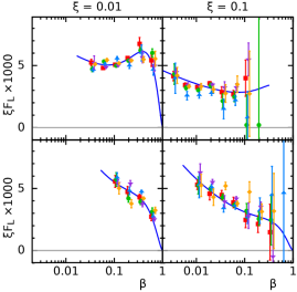
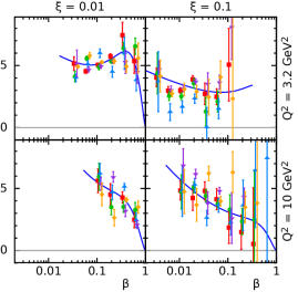
$E_{\mathrm{CM}}\textrm{ set S-9},\delta_{\mathrm{sys}}=1\%,68\%\ {\rm CL}$	$E_{\mathrm{CM}}\textrm{ set S-5},\delta_{\mathrm{sys}}=1\%,68\%\ {\rm CL}$

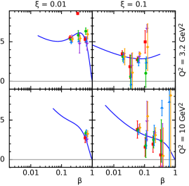
Figure 8: Comparisons of the extracted $F_{\mathrm{L}}^{\mathrm{D(3)}}$ in four selected $(\xi,Q^{2})$ bins, for five Monte Carlo samples (markers with different colours, horizontally displaced from each other for clarity). The first row compares the results for two different $\delta_{\mathrm{sys}}$ values, 1% on the left and 2% on the right, for the S-17 set of beam energies. In the second row the results for smaller $E_{\mathrm{CM}}$ sets (S-9 and S-5) are shown with $\delta_{\mathrm{sys}}=1\%$. The solid lines show the central values of the model used for the generation of the pseudodata from which $F_{\mathrm{L}}^{\mathrm{D(3)}}$ was extracted.

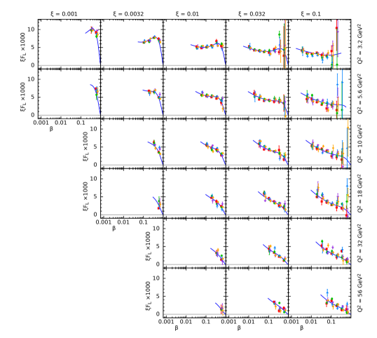
Figure 9: Extracted $F_{\mathrm{L}}^{\mathrm{D(3)}}$ for set S-17, $\delta_{\mathrm{sys}}$=1%, 68% CL uncertainty bands, for 5 MC samples (markers with different colours, horizontally displaced from each other for clarity). The solid lines show the central values of the model used for the generation of the pseudodata from which $F_{\mathrm{L}}^{\mathrm{D(3)}}$ was extracted.

4.2 Estimated precision on $F_{\mathrm{L}}^{\mathrm{D(3)}}$

Figs. 8 and 9 illustrate the spread of results for $F_{\mathrm{L}}^{\mathrm{D(3)}}$ extracted from 68% CL uncertainties on fits to five different Monte Carlo pseudodata samples generated using the same central values and uncertainties. The resulting distributions at each $(Q^{2},\beta,\xi)$ point are complicated, since in addition to the uncertainties propagated through the fits from the pseudodata, they also reflect the available $Y_{\mathrm{L}}$ range and number of data points available in the fits. In order to estimate the precision with which $F_{\mathrm{L}}^{\mathrm{D(3)}}$ can be extracted at each $(Q^{2},\beta,\xi)$ point, we investigate the spread between the results obtained with the different Monte Carlo samples, quantified using a direct arithmetic averaging procedure, neglecting the uncertainties obtained from the fits. The mean and variance are therefore taken to be

$$\bar{v}=S_{1}/N,\quad(\Delta v)^{2}=\frac{S_{2}-S_{1}^{2}/N}{N-1}\ ,$$ (15)

with $S_{n}=\sum_{i=1}^{N}v_{i}^{n}$ and $v_{i}$ the value of the extracted $\xi$$F_{\mathrm{L}}^{\mathrm{D(3)}}$ in Monte Carlo sample $i$. The uncertainty is then taken to be $\Delta v$.

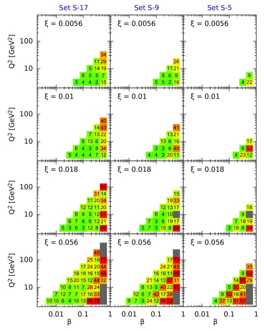
Figure 10: Estimated uncertainties $\Delta v$ on $F_{\mathrm{L}}^{\mathrm{D(3)}}$ extractions for beam energy sets S-17, S-9, S-5, averaged over 10 MC samples for $\delta_{\mathrm{sys}}$ = 1%. The numbers in each box give the relative accuracy of the $F_{\mathrm{L}}^{\mathrm{D(3)}}$ determination (in percent). Bins with errors exceeding 100% are indicated in grey.

Fig. 10 shows the uncertainties $\Delta v$ in ($\beta,Q^{2},\xi$) bins for the three sets of beam energies, obtained by averaging over 10 separate Monte Carlo simulations. Even with 10 MC samples, there are some strong point-to-point fluctuations in the estimated uncertainties. However, the general trends become clear, in particular the regions in which reliable measurements can be made. The best measured region for each $\xi$ value is at the lowest $\beta$ and $Q^{2}$, where the $Y_{\mathrm{L}}$ range is widest and statistical errors are negligible. The uncertainties in a given bin do not depend strongly on the energy sets, but the accessible kinematic range in which measurements can be made decreases with decreasing numbers of energy combinations in the set.

4.3 Results for the ratio of the longitudinal to transverse structure functions

The ‘photoabsorption’ ratio in diffraction, $R^{\rm D(3)}=F_{\mathrm{L}}^{\mathrm{D(3)}}/F_{\mathrm{T}}^{\mathrm{D(3)}}$, where $F_{\mathrm{T}}^{\mathrm{D(3)}}=F_{2}^{\mathrm{D(3)}}-F_{\mathrm{L}}^{\mathrm{D(3)}}$, is the ratio of the cross section for longitudinally polarised photons to that for transversely polarised photons at the same $(\beta,Q^{2},\xi)$ values. $R^{\rm D(3)}$ has a clear and intuitive physical meaning and can be compared with similar quantities extracted from decay angular distributions in exclusive processes such as vector meson production. It can be extracted from a fit to the reduced cross section pseudodata as a function of $Y_{\mathrm{L}}$ of the form

$$\sigma_{\mathrm{red}}^{\mathrm{D}(3)}=\left[1+\left(1-Y_{\mathrm{L}}\right)\,R^{\rm D(3)}\right]F_{\mathrm{T}}^{\mathrm{D(3)}}\;,$$ (16)

with $R^{\rm D(3)}$ and $F_{\mathrm{T}}^{\mathrm{D(3)}}$ being the free fit parameters. This alternative fit has different sensitivities to the uncertainties in the measurements from those in the $F_{\mathrm{L}}^{\mathrm{D(3)}}$ extraction.

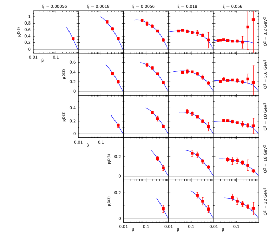
Figure 11: Extracted $R^{\rm D(3)}$ data for beam energy set S-17 averaged over 10 MC samples with $\delta_{\mathrm{sys}}$ = 1%. The solid lines show the central values of the model used for the generation of the pseudodata.

Fig. 11 shows the results for the values of $R^{\rm D(3)}$ obtained from the averaging method described in Sec. 4.2 using 10 Monte Carlo samples and the largest set of beam energies, S-17 and $\delta_{\mathrm{sys}}$ = 1%. A precise determination of $R^{\rm D(3)}$ over a large kinematic range will be possible at the EIC.

5 Conclusions and Outlook

In this paper we have investigated the potential of the Electron Ion Collider for the measurement of the longitudinal structure function in diffraction. This is a challenging measurement that requires data with high statistics at several different centre-of-mass energies, ideally well beyond those available in the pioneering measurement by the H1 collaboration at HERA. We have considered EIC scenarios with 17, 9 and 5 different values of $\sqrt{s}$, the latter being the commonly assumed EIC scenario. Pseudodata for the reduced diffractive cross section were generated using a model based on collinear factorization with DGLAP evolution, assuming an integrated luminosity of $10\,\rm fb^{-1}$ for each centre-of-mass energy. The uncorrelated systematic errors are assumed to be either $1\%$ or $2\%$, which is challenging compared with previous measurements, but consistent with the expected high level of performance of the EIC detectors. The longitudinal structure function was extracted using the standard Rosenbluth method of a linear fit to the reduced cross section as a function of the $Y_{\mathrm{L}}$ variable, extracting $F_{\mathrm{L}}^{\mathrm{D(3)}}$ from the slope and $F_{2}^{\mathrm{D}(3)}$ from the intercept. Fits were only performed in $(\beta,\xi,Q^{2})$ bins where at least four centre-of-mass energies yielded data points at accessible $y$ values (in contrast to three in the H1 case). The scenarios with 17 and 9 centre-of-mass energies do not differ much in terms of the kinematic range in which $F_{\mathrm{L}}^{\mathrm{D(3)}}$ can be extracted, whereas the scenario with only 5 centre-of-mass energies results in a restricted kinematic range, particularly at small values of $\beta$ and $\xi$. The precision on the extracted value of $F_{\mathrm{L}}^{\mathrm{D(3)}}$ is strongly correlated with the available range in $Y_{\mathrm{L}}$ in a given bin $(\xi,\beta,Q^{2})$ and is not diminished substantially when going from 17 to 9 centre-of-mass energies. A larger difference is observed for the set with 5 centre-of-mass energies, mainly due to the smaller available range in $y$. Nonetheless, for bins in which measurements are possible, the precision of the extracted structure function $F_{\mathrm{L}}^{\mathrm{D(3)}}$ is comparable in all scenarios. Given the very high target luminosity at the EIC, the exact choices of running time at each beam energy will not be a strongly limiting factor; the precision is likely to depend much more strongly on the size of the systematic uncertainties that are not correlated between data points.

We have also performed a separate extraction of the ratio $R^{\rm D(3)}=F_{\mathrm{L}}^{\mathrm{D(3)}}/(F_{2}^{\mathrm{D(3)}}-F_{\mathrm{L}}^{\mathrm{D(3)}})$ of the longitudinal to the transverse diffractive structure functions. A precise extraction of this quantity is expected to be possible at the EIC.

As an outlook, we note that the currently foreseen forward instrumentation at the EIC allows a precise determination of $-t$ in a wide range, see Sec. 2.2. It will be very interesting to explore to what extent an extraction of $F_{\mathrm{L}}^{\mathrm{D}(4)}(\beta,\xi,Q^{2},t)$ in a similar way to that illustrated previously for $F_{\mathrm{L}}^{\mathrm{D(3)}}$, Eq. (4), will be possible. This is a completely new study that we leave for the future.

References

- [1] C. Adloff et al. Inclusive measurement of diffractive deep inelastic ep scattering. Z. Phys., C76:613–629, 1997.
- [2] J. Breitweg et al. Measurement of the diffractive structure function at HERA. Eur. Phys. J., C1:81–96, 1998.
- [3] P. Newman and M. Wing. The Hadronic Final State at HERA. Rev. Mod. Phys., 86(3):1037, 2014.
- [4] A. Aktas et al. Diffractive deep-inelastic scattering with a leading proton at HERA. Eur.Phys.J., C48:749–766, 2006.
- [5] F. D. Aaron et al. Measurement of the cross section for diffractive deep-inelastic scattering with a leading proton at HERA. Eur. Phys. J. C, 71:1578, 2011.
- [6] S. Chekanov et al. Dissociation of virtual photons in events with a leading proton at HERA. Eur. Phys. J. C, 38:43–67, 2004.
- [7] S. Chekanov et al. Deep inelastic scattering with leading protons or large rapidity gaps at HERA. Nucl. Phys. B, 816:1–61, 2009.
- [8] A. Aktas et al. Measurement and QCD analysis of the diffractive deep-inelastic scattering cross-section at HERA. Eur. Phys. J. C, 48:715–748, 2006.
- [9] F. D. Aaron et al. Inclusive Measurement of Diffractive Deep-Inelastic Scattering at HERA. Eur. Phys. J. C, 72:2074, 2012.
- [10] S. Chekanov et al. A QCD analysis of ZEUS diffractive data. Nucl.Phys., B831:1–25, 2010.
- [11] A. B. Kaidalov. Diffractive Production Mechanisms. Phys. Rept., 50:157–226, 1979.
- [12] A. B. Kaidalov, V. A. Khoze, A. D. Martin, and M. G. Ryskin. Diffraction of protons and nuclei at high-energies. Acta Phys. Polon. B, 34:3163–3190, 2003.
- [13] J. Bartels and H. Kowalski. Diffraction at HERA and the confinement problem. Eur. Phys. J. C, 19:693–708, 2001.
- [14] Y. V. Kovchegov and E. Levin. Quantum chromodynamics at high energy, volume 33. Cambridge University Press, 8 2012.
- [15] V. N. Gribov. Glauber corrections and the interaction between high-energy hadrons and nuclei. Sov. Phys. JETP, 29:483–487, 1969. [Zh. Eksp. Teor. Fiz.56,892(1969)].
- [16] J. C. Collins. Proof of factorization for diffractive hard scattering. Phys. Rev., D57:3051–3056, 1998. [Erratum: Phys. Rev.D61,019902(2000)].
- [17] A. Berera and D. E. Soper. Behavior of diffractive parton distribution functions. Phys. Rev., D53:6162–6179, 1996.
- [18] L. Trentadue and G. Veneziano. Fracture functions: An Improved description of inclusive hard processes in QCD. Phys. Lett., B323:201–211, 1994.
- [19] M. Klasen and G. Kramer. Review of factorization breaking in diffractive photoproduction of dijets. Mod. Phys. Lett. A, 23:1885–1907, 2008.
- [20] K. Akiba et al. LHC Forward Physics. J. Phys. G, 43:110201, 2016.
- [21] L. Motyka, M. Sadzikowski, and W. Slominski. Evidence of strong higher twist effects in diffractive DIS at HERA at moderate . Phys. Rev., D86:111501, 2012.
- [22] F. D. Aaron et al. Measurement of the Diffractive Longitudinal Structure Function at HERA. Eur. Phys. J. C, 71:1836, 2011.
- [23] A. Accardi et al. Electron Ion Collider: The Next QCD Frontier. Eur. Phys. J., A52(9):268, 2016.
- [24] R. Abdul Khalek et al. Science Requirements and Detector Concepts for the Electron-Ion Collider: EIC Yellow Report. 3 2021.
- [25] J. L. Abelleira Fernandez et al. A Large Hadron Electron Collider at CERN: Report on the Physics and Design Concepts for Machine and Detector. J. Phys., G39:075001, 2012.
- [26] P. Agostini et al. The Large Hadron-Electron Collider at the HL-LHC. 7 2020.
- [27] A. Abada et al. FCC Physics Opportunities: Future Circular Collider Conceptual Design Report Volume 1. Eur. Phys. J. C, 79(6):474, 2019.
- [28] A. Abada et al. FCC-hh: The Hadron Collider: Future Circular Collider Conceptual Design Report Volume 3. Eur. Phys. J. ST, 228(4):755–1107, 2019.
- [29] N. Armesto, P. R. Newman, W. Słomiński, and A. M. Staśto. Inclusive diffraction in future electron-proton and electron-ion colliders. Phys. Rev. D, 100(7):074022, 2019.
- [30] W. Slominski, N. Armesto, P. R. Newman, and A. Stasto. Opportunities for inclusive diffraction at EIC. 7 2021.
- [31] S. Chekanov et al. Study of deep inelastic inclusive and diffractive scattering with the ZEUS forward plug calorimeter. Nucl. Phys., B713(1-3):3–80, 2005.
- [32] A. Aktas et al. Measurement and QCD analysis of the diffractive deep-inelastic scattering cross-section at HERA. Eur.Phys.J., C48:715–748, 2006.
- [33] S. Chekanov et al. Deep inelastic scattering with leading protons or large rapidity gaps at HERA. Nucl.Phys., B816:1–61, 2009.
- [34] F.D. Aaron et al. Inclusive Measurement of Diffractive Deep-Inelastic Scattering at HERA. Eur.Phys.J., C72:2074, 2012.
- [35] V. N. Gribov and L. N. Lipatov. pair annihilation and deep inelastic e p scattering in perturbation theory. Sov. J. Nucl. Phys., 15:675–684, 1972. [Yad. Fiz.15,1218(1972)].
- [36] V. N. Gribov and L. N. Lipatov. Deep inelastic e p scattering in perturbation theory. Sov. J. Nucl. Phys., 15:438–450, 1972. [Yad. Fiz.15,781(1972)].
- [37] G. Altarelli and G. Parisi. Asymptotic Freedom in Parton Language. Nucl. Phys., B126:298–318, 1977.
- [38] Y. L. Dokshitzer. Calculation of the Structure Functions for Deep Inelastic Scattering and Annihilation by Perturbation Theory in Quantum Chromodynamics. Sov. Phys. JETP, 46:641–653, 1977. [Zh. Eksp. Teor. Fiz.73,1216(1977)].
- [39] M. Derrick et al. Study of elastic photoproduction at HERA using the ZEUS leading proton spectrometer. Z. Phys. C, 73:253–268, 1997.
- [40] P. Van Esch et al. The H1 forward proton spectrometer at HERA. Nucl. Instrum. Meth. A, 446:409–425, 2000.
- [41] A. Astvatsatourov, K. Cerny, J. Delvax, L. Favart, T. Hreus, X. Janssen, R. Roosen, T. Sykora, and P. Van Mechelen. The H1 very forward proton spectrometer at HERA. Nucl. Instrum. Meth. A, 736:46–65, 2014.
- [42] S. Abdel Khalek et al. The ALFA Roman Pot Detectors of ATLAS. JINST, 11(11):P11013, 2016.
- [43] L Adamczyk, E Banaś, A Brandt, M Bruschi, S Grinstein, J Lange, M Rijssenbeek, P Sicho, R Staszewski, T Sykora, M Trzebiński, J Chwastowski, and K Korcyl. Technical Design Report for the ATLAS Forward Proton Detector. Technical report, May 2015.
- [44] G. Antchev et al. First measurement of elastic, inelastic and total cross-section at TeV by TOTEM and overview of cross-section data at LHC energies. Eur. Phys. J. C, 79(2):103, 2019.
- [45] Albert M Sirunyan et al. Observation of proton-tagged, central (semi)exclusive production of high-mass lepton pairs in pp collisions at 13 TeV with the CMS-TOTEM precision proton spectrometer. JHEP, 07:153, 2018.
- [46] S. Chekanov et al. A QCD analysis of ZEUS diffractive data. Nucl. Phys. B, 831:1–25, 2010.
- [47] J. C. Collins and W.-K. Tung. Calculating Heavy Quark Distributions. Nucl. Phys., B278:934, 1986.
- [48] R. S. Thorne and W. K. Tung. PQCD Formulations with Heavy Quark Masses and Global Analysis. 2008.
- [49] J. F. Owens. Dependent Parametrizations of Pion Parton Distribution Functions. Phys. Rev., D30:943, 1984.
- [50] M. Gluck, E. Reya, and A. Vogt. Pionic parton distributions. Z. Phys., C53:651–656, 1992.
- [51] H. Jung. Hard diffractive scattering in high-energy e p collisions and the Monte Carlo generator RAPGAP. Comput. Phys. Commun., 86:147–161, 1995.
- [52] F. D. Aaron et al. Measurement of the Proton Structure Function (x, ) at Low x. Phys. Lett. B, 665:139–146, 2008.
- [53] S. Chekanov et al. Measurement of the Longitudinal Proton Structure Function at HERA. Phys. Lett. B, 682:8–22, 2009.
- [54] F. D. Aaron et al. Measurement of the Inclusive p Scattering Cross Section at High Inelasticity y and of the Structure Function . Eur. Phys. J. C, 71:1579, 2011.