Loop induced $h\rightarrow\gamma\gamma,Z\gamma,gg$ decays in 3-Higgs doublet models

Abstract

Abstract

In this paper, we analyze the loop induced decays of neutral Higgs boson $h$ into pairs of photons, gluons, and Z$\gamma$ in 3-Higgs Doublet Models (3HDMs), where all the doublets have non-zero vacuum expectation values. In the 3HDM, there are contributions to these decays from loops of charged scalars $H^{\pm}_{1,2}$ that are not present in the Standard Model. We find an enhancement in the channel $h\rightarrow Z\gamma$ with respect to the Standard Model prediction in some parameter region while respecting constraints from the measurements of $h\rightarrow\gamma\gamma$ at the LHC. The charged Higgs bosons $H^{\pm}_{1,2}$ lead to the enhancement of $Z\gamma$ decay mode in some part of the parameter space of the 3HDM. Then, we discuss the correlations between the decay modes $h\rightarrow Z\gamma$ and $h\rightarrow\gamma\gamma$. Moreover, we study Type-I and Type-Z of 3HDMs and find that these types of 3HDMs can be distinguished via only the gluonic decays, since the contributions of the $H^{\pm}_{1,2}$ loops are dominant to those of fermion loops. We also investigate the effects of the model parameters on these loop induced decays. As an interesting phenomenological consequence, the 3HDM is dominantly governed by the parameters: two ratios of vacuum expectation values (VEVs); $\tan\gamma,~{}\tan\beta$ and the mixing angles of the CP-even Higgs bosons, $\alpha_{1,2}~{}\text{and}~{}\theta$.

I Introduction

Recently a Higgs boson with a mass of 125 GeV has been discovered at the Large Hadron Collider (LHC) Aad:2012tfa ; Chatrchyan:2012xdj that resembles the Standard Model (SM) Higgs boson. This discovery, however raises one important question, whether it is indeed the SM Higgs boson or a Higgs boson of new physics beyond the SM. In the class of the many beyond SM scenarios, an interesting class of Higgs-sector extension is the n-Higgs Doublet Model (nHDM). One of the simplest but important examples is the two-Higgs-doublet model (2HDM) with one additional scalar doublet Branco:2011iw ; Bhattacharyya:2015nca . In recent years, a lot of attention has been given to the Three Higgs Doublet Model (3HDM) with additional two Higgs doublets my3hdm ; 3hdm ; 3hdm1 ; 3hdm2 ; 3hdm3 ; 3hdm4 ; 3hdm5 ; 3hdm6 ; Yagyu:2016whx ; Ferreira:2008zy ; Machado:2010uc ; Ivanov:2012ry ; GonzalezFelipe:2013xok ; GonzalezFelipe:2013yhh ; Keus:2013hya ; Ivanov:2014doa ; Maniatis:2014oza ; 3hdm-uni ; Das:2019yad . Extended Higgs sectors naturally give rise to Flavor-Changing Neutral Currents (FCNCs) which are in conflict with various flavour data at the tree level. This problem is usually avoided by implementing discrete symmetries in the Yukawa interactions. For example, in the 3HDM, only one of the three doublets couples to each type of fermion. The rich particle spectrum of the 3HDM consists of three CP-even Higgs bosons, $h$, $H_{1}$ and $H_{2}$, two CP-odd Higgs bosons, $A_{1}$ and $A_{2}$; and two pair of charged Higgs bosons, $H^{\pm}_{1}$ and $H^{\pm}_{2}$. In this paper, we discuss the possibility that the discovered Higgs boson at the LHC is the lightest CP-even neutral Higgs boson $h$ of the 3HDM.

In this paper, we study the loop-induced decays $h\rightarrow\gamma\gamma$, $Z\gamma$ and $gg$ in the 3HDM and their behavior over the model parameters. The loop induced processes are sensitive to new physics contributions, which would interfere with the SM contributions. Although a large number of works have investigated the effects of new particles in the loop induced decay widths of the Higgs 3hdm ; 3hdm3 ; loop ; loop2 ; loop3 ; Aranda:2013kq ; Fontes:2014xva ; Arhrib:2011vc ; Hammad:2015eca , a systematic numerical study of the 3HDM loop induced decay widths are still missing. In particular, we will study under which circumstances, the loop induced decay widths could be significantly affected. We consider the possibility of constructive interference of the $H^{\pm}_{1}$ and $H^{\pm}_{2}$ contributions with the SM particles contributions due to enhancement of the decay widths $h\rightarrow Z\gamma$ in the 3HDM. Besides the two ratios of Vacuum Expectation Values (VEVs), $\tan\beta$ and $\tan\gamma$, all loop induced decay widths are quite sensitive to parameters $\alpha_{1,2}$ and $\theta$, which are the mixing angles between the CP even Higgs bosons.

We will examine constraints on the parameter spaces of the Type-I and Type-Z- 3HDM by taking into account the measured value of $h\rightarrow\gamma\gamma$ decay at the LHC. Then, we will investigate whether an enhancement in the $h\rightarrow Z\gamma$ decay mode exists while respecting these constraints. We obtain an enhancement in the $h\rightarrow Z\gamma$ decay mode in part of the parameter space. Archer-Smith et al. recently investigated the decay rate of $h\rightarrow Z\gamma$ and found that simple models cannot lead to large enhancements while still respecting other data, particularly measurements of $h\rightarrow\gamma\gamma$ Archer-Smith:2020gib . According to Ref. Chen:2013vi , the $h\rightarrow Z\gamma$ decay rate can enhance or reduce with respect to its SM value: $0.76<\Gamma(h\rightarrow Z\gamma)/\Gamma(h\rightarrow Z\gamma)_{SM}<2.05.$ In a study in the context of an Inert Triplet Model (ITP) in Ref. Kanemura:2018esc , the $h\rightarrow Z\gamma$ decay is suppressed by about 70 % from the SM prediction, while the $h\rightarrow\gamma\gamma$ decay remains as in the SM. Wang et al. investigated the $h\rightarrow\gamma\gamma$ decay in a 2HDM, but the partial decay width $\Gamma(h\rightarrow Z\gamma)$ is generally less than the SM expectation Wang:2017xml .

The correlation between $h\rightarrow\gamma\gamma$ and $h\rightarrow Z\gamma$ has been examined in some Refs.loop2 ; BhupalDev:2013xol ; Chen:2013dh ; Chiang:2012qz ; Chen:2013vi ; Chabab:2018ert . An interesting thing is that correlations between the $h\rightarrow\gamma\gamma$ and $h\rightarrow Z\gamma$ decays appear in some parameter space in our model by imposing the $h\rightarrow\gamma\gamma$ decay measured by the LHC.

In particular, we study the Type-I and Type-Z 3HDM among the five Yukawa types of 3HDMs. However, one can distinguish these Yukawa types in in gluonic decay modes. Only heavy quark loops contribute to the gluonic decays, while additional new charged Higgs bosons $H^{\pm}_{1,2}$ enter the loop in the $\gamma\gamma$ and $Z\gamma$ decay modes as well as the SM particles. The heavy quark contributions are small compared to new charged Higgs bosons contributions in the $\gamma\gamma$ and $Z\gamma$ mode, hence Yukawa types in the 3HDM could not be distinguished in these decay modes. In general, one of the most important parameters to distinguish different Yukawa types in the 3HDM is denoted as $\tan\beta$ and $\tan\gamma$. The gluonic and photonic decay widths are significant to investigate the Higgs production at hadron and photon colliders, where the cross sections will be directly proportional to, respectively, the gluonic and photonic decay widths.

Our work is organized as follows. In section II, we briefly describe the theoretical structure of the 3HDM. In section III, we present the couplings of the particles in the 3HDM relevant to our calculation. Analytic formulas needed for calculating the decay widths of the $h\rightarrow\gamma\gamma,~{}\gamma Z,~{}gg$ are presented in section IV, and we discuss the numerical results of the partial decay widths and branching ratios in the 3HDM. We finally summarize our results in section V. In the appendix, we collect expressions for the loop functions used in our calculations. Moreover, details on the analysis of the scalar potential and the coefficients of the triple scalar couplings are given in the appendix.

II Three Higgs Doublet Model

Yukawa Types	$\Phi_{u}$	$\Phi_{d}$	$\Phi_{e}$
Type-I	$\Phi_{2}$	$\Phi_{2}$	$\Phi_{2}$
Type-II	$\Phi_{2}$	$\Phi_{1}$	$\Phi_{1}$
Type-X	$\Phi_{2}$	$\Phi_{2}$	$\Phi_{1}$
Type-Y	$\Phi_{2}$	$\Phi_{1}$	$\Phi_{2}$
Type-Z	$\Phi_{2}$	$\Phi_{1}$	$\Phi_{3}$

Table 1: The five physically-distinct types of Yukawa interactions under the $Z_{2}\times\tilde{Z}_{2}$ symmetries my3hdm .

	Factor for $\tilde{H}_{1}$, $\tilde{A}_{1}$ and $\tilde{H}_{1}^{\pm}$			Factor for $\tilde{H}_{2}$, $\tilde{A}_{2}$ and $\tilde{H}_{2}^{\pm}$
	$R_{u2}/R_{u1}$	$R_{d2}/R_{d1}$	$R_{e2}/R_{e1}$	$R_{u3}/R_{u1}$	$R_{d3}/R_{d1}$	$R_{e3}/R_{e1}$
Type-I	$\cot\beta$	$\cot\beta$	$\cot\beta$	0	0	0
Type-II	$\cot\beta$	$-\tan\beta$	$-\tan\beta$	0	$-\tan\gamma/\cos\beta$	$-\tan\gamma/\cos\beta$
Type-X	$\cot\beta$	$\cot\beta$	$-\tan\beta$	0	0	$-\tan\gamma/\cos\beta$
Type-Y	$\cot\beta$	$-\tan\beta$	$\cot\beta$	0	$-\tan\gamma/\cos\beta$	0
Type-Z	$\cot\beta$	$-\tan\beta$	$-\tan\beta$	0	$-\tan\gamma/\cos\beta$	$\cot\gamma/\cos\beta$

Table 2: Factors appearing in Eq. (15) for each type of Yukawa interaction.

The most general Higgs potential invariant under the $SU(2)_{L}\times U(1)_{Y}\times Z_{2}\times\tilde{Z}_{2}$ symmetry is expressed by my3hdm

$$V(\Phi_{1},\Phi_{2},\Phi_{3}) =\sum_{i=1}^{3}m_{i}^{2}\Phi_{i}^{\dagger}\Phi_{i}-(m_{12}^{2}\Phi_{1}^{\dagger}\Phi_{2}+m_{13}^{2}\Phi_{1}^{\dagger}\Phi_{3}+m_{23}^{2}\Phi_{2}^{\dagger}\Phi_{3}+\text{h.c.})$$

$$+\frac{1}{2}\sum_{i=1}^{3}\lambda_{i}(\Phi_{i}^{\dagger}\Phi_{i})^{2}+\rho_{1}(\Phi_{1}^{\dagger}\Phi_{1})(\Phi_{2}^{\dagger}\Phi_{2})+\rho_{2}|\Phi_{1}^{\dagger}\Phi_{2}|^{2}+\frac{1}{2}[\rho_{3}(\Phi_{1}^{\dagger}\Phi_{2})^{2}+\text{h.c.}]$$

$$+\sigma_{1}(\Phi_{1}^{\dagger}\Phi_{1})(\Phi_{3}^{\dagger}\Phi_{3})+\sigma_{2}|\Phi_{1}^{\dagger}\Phi_{3}|^{2}+\frac{1}{2}[\sigma_{3}(\Phi_{1}^{\dagger}\Phi_{3})^{2}+\text{h.c.}]$$

$$+\kappa_{1}(\Phi_{2}^{\dagger}\Phi_{2})(\Phi_{3}^{\dagger}\Phi_{3})+\kappa_{2}|\Phi_{2}^{\dagger}\Phi_{3}|^{2}+\frac{1}{2}[\kappa_{3}(\Phi_{2}^{\dagger}\Phi_{3})^{2}+\text{h.c.}],$$ (1)

where we allow the presence of the soft breaking terms $m_{12}^{2}$, $m_{13}^{2}$ and $m_{23}^{2}$ for the discrete $Z_{2}$ symmetries. To avoid explicit CP violation, we take all the parameters of the scalar potential to be real.

In order to suppress FCNCs at tree level, we will enforce each type of fermion to couple to only a single Higgs doublet in the Yukawa sector. In the 3HDM, this condition leads to the five physically-distinct “types” given in Tab. 1. The Yukawa Lagrangian of the 3HDM reads

$$-{\cal L}_{Y}=Y_{u}\bar{Q}_{L}(i\sigma_{2})\Phi_{u}^{*}u_{R}+Y_{d}\bar{Q}_{L}\Phi_{d}d_{R}+Y_{e}\bar{L}_{L}\Phi_{e}e_{R}+\text{h.c.},$$ (2)

where $\Phi_{u,d,e}$ are either $\Phi_{1}$, $\Phi_{2}$ or $\Phi_{3}$.

The general 3HDM contains three scalar $SU(2)_{L}$ doublet fields, denoted here as

$$\Phi_{i}=\left[\begin{array}[]{cc}\omega_{i}^{+}\\ \frac{1}{\sqrt{2}}(h_{i}+v_{i}+iz_{i})\end{array}\right],~{}~{}(i=1,...3),$$ (5)

where the $v_{i}$’s are the VEVs of the $\Phi_{i}$’s with the sum rule $\sum_{i}v_{i}^{2}\equiv v^{2}=1/(\sqrt{2}G_{F})\simeq(246$ GeV$)^{2}$. The VEVs may be introduced by the two ratios

$$\tan\beta\equiv\frac{v_{2}}{v_{13}},\quad\tan\gamma\equiv\frac{v_{3}}{v_{1}},~{}~{}\text{with}~{}~{}v_{13}\equiv\sqrt{v_{1}^{2}+v_{3}^{2}}.$$ (6)

Using this notation, each of the VEVs is parametrized by

$$v_{1}=v_{13}\cos\gamma=v\cos\beta\cos\gamma,\quad v_{2}=v\sin\beta,\quad v_{3}=v_{13}\sin\gamma=v\cos\beta\sin\gamma.$$ (7)

Scalar mass eigenstates can be obtained by rotating the fields. The rotation is performed in two stages. The first stage is to transform all scalar fields from a weak basis with a generic choice of vacua to the so-called Higgs basis higgsbasis ; higgsbasis2 , where only 1-Higgs doublet contains the SM VEV $v$ and the Nambu-Goldstone (NG) bosons. This can be done by rotating to the Higgs basis using the orthogonal $3\times 3$ matrix $R$ as follows:

$$\begin{pmatrix}h_{1}\\ h_{2}\\ h_{3}\end{pmatrix}=R\begin{pmatrix}\tilde{h}\\ \tilde{H_{1}}\\ \tilde{H_{2}}\end{pmatrix},~{}\begin{pmatrix}w_{1}^{\pm}\\ w^{\pm}_{2}\\ w^{\pm}_{3}\end{pmatrix}=R\begin{pmatrix}G^{\pm}\\ \tilde{H^{\pm}_{1}}\\ \tilde{H_{2}^{\pm}}\end{pmatrix},~{}\begin{pmatrix}z_{1}\\ z_{2}\\ z_{3}\end{pmatrix}=R\begin{pmatrix}G^{0}\\ \tilde{A_{1}}\\ \tilde{A_{2}}\end{pmatrix}.$$ (8)

The $R$ matrix is expressed in terms of the three VEVs, following the notation of Ref. my3hdm

$$R =\begin{pmatrix}\frac{v_{1}}{v}&-\frac{v_{2}v_{1}}{v_{13}v}&-\frac{v_{3}}{v_{13}}\\ \frac{v_{2}}{v}&\frac{v_{13}}{v}&0\\ \frac{v_{3}}{v}&-\frac{v_{2}v_{3}}{v_{13}v}&\frac{v_{1}}{v_{13}}\end{pmatrix}=\begin{pmatrix}\cos\gamma&0&-\sin\gamma\\ 0&1&0\\ \sin\gamma&0&\cos\gamma\\ \end{pmatrix}\begin{pmatrix}\cos\beta&-\sin\beta&0\\ \sin\beta&\cos\beta&0\\ 0&0&1\end{pmatrix}$$

$$=\begin{pmatrix}\cos\beta\cos\gamma&-\sin\beta\cos\gamma&-\sin\gamma\\ \sin\beta&\cos\beta&0\\ \cos\beta\sin\gamma&-\sin\beta\sin\gamma&\cos\gamma\end{pmatrix}.$$ (9)

After spontaneous symmetry breaking (SSB), the NG bosons $G^{\pm}$ and $G^{0}$ are absorbed into the longitudinal components of the $W^{\pm}$ and $Z$ respectively. In Eq. (6), two singly-charged states $\tilde{H}_{a}^{\pm}$, two CP-odd states $\tilde{A}_{a}$ and three CP-even states $\tilde{h}$ and $\tilde{H}_{a}$ are not given in the mass eigenstates. The next stage is to determine the scalar mass eigenstates through the orthogonal transformations

$$\begin{pmatrix}G^{\pm}\\ H^{\pm}_{1}\\ H_{2}^{\pm}\end{pmatrix}=O_{c}^{\dagger}\begin{pmatrix}w^{\pm}_{1}\\ w^{\pm}_{2}\\ w^{\pm}_{3}\end{pmatrix},~{}O_{\theta_{2}}=\begin{pmatrix}1&0&0\\ 0&\cos(\theta_{2})&-\sin(\theta_{2})\\ 0&\sin(\theta_{2})&\cos(\theta_{2})\\ \end{pmatrix}$$ (10)

$$\begin{pmatrix}G^{0}\\ A_{1}\\ A_{2}\end{pmatrix}=O^{\dagger}_{A}\begin{pmatrix}z_{1}\\ z_{2}\\ z_{3}\end{pmatrix},~{}O_{\theta_{1}}=\begin{pmatrix}1&0&0\\ 0&\cos(\theta_{1})&-\sin(\theta_{1})\\ 0&\sin(\theta_{1})&\cos(\theta_{1})\\ \end{pmatrix},$$ (11)

where $\theta_{2}$ and $\theta_{1}$ are the mixing angles for the charged and CP-odd states, respectively. $O_{c}=O_{\theta_{2}}R,~{}~{}O_{A}=O_{\theta_{1}}R.$

For the CP-even states, we can obtain the mass eigenstates through

$$\begin{pmatrix}\tilde{h}_{1}\\ \tilde{H}_{1}\\ \tilde{H}_{2}\end{pmatrix}=O^{h}\begin{pmatrix}h\\ H_{1}\\ H_{2}\end{pmatrix}.$$ (12)

where $O^{h}=R^{T}O$ and

$$O=R_{23}(\theta)R_{12}(\alpha_{1})R_{13}(\alpha_{2})$$ (13)

where $\alpha_{1,2},~{}\theta$ mixing angles in the CP-even sector.

$$R_{13}(\alpha_{2})=\begin{pmatrix}\cos\alpha_{2}&-\sin\alpha_{2}&0\\ \sin\alpha_{2}&\cos\alpha_{2}&0\\ 0&0&1\end{pmatrix},~{}R_{12}(\alpha_{1})=\begin{pmatrix}\cos\alpha_{1}&0&-\sin\alpha_{1}\\ 0&1&0\\ \sin\alpha_{1}&0&\cos\alpha_{1}\end{pmatrix},~{}R_{23}(\theta)=\begin{pmatrix}1&0&0\\ 0&\cos(\theta)&-\sin(\theta)\\ 0&\sin(\theta)&\cos(\theta)\\ \end{pmatrix}.$$ (14)

The masses of the three neutral physical states, $h,$ $H_{1}$ and $H_{2}$, are evaluated in detail in Appendix A.3. Consequently, the model has nine scalar physical particles: (i) three CP-even scalars $(h,H_{1,2}),$ (ii) two CP-odd scalars $(A_{1,2}),$ and (iii) four charged scalars$(H^{\pm}_{1,2}).$ In this paper, we focus on the physics related to the Higgs bosons $h,~{}H_{1},~{}H_{2}$, $H_{1}^{\pm}$ and $H_{2}^{\pm}$, for which there are eighteen significant parameters, namely

$$m_{h},~{}m_{H_{1}},~{}m_{H_{2}},~{}m_{H_{1}^{\pm}},~{}m_{H_{2}^{\pm}},~{}m_{A_{1}},~{}m_{A_{2}},~{}v,~{}\tan\beta,~{}\tan\gamma,~{}\theta_{1},~{}\theta_{2},~{}\alpha_{1,2},~{}\theta,m_{12},~{}m_{23},~{}\text{and}~{}m_{13}.$$

II.1 The Yukawa sector

The Yukawa couplings of the Higgs bosons are given by my3hdm

$$-{\cal L}_{Y}=\sum_{f=u,d,e}\frac{m_{f^{i}}}{v}\bar{f}^{i}\left[\left(\tilde{h}+\frac{R_{f2}}{R_{f1}}\tilde{H}_{1}+\frac{R_{f3}}{R_{f1}}\tilde{H_{2}}\right)-2I_{f}\left(\frac{R_{f2}}{R_{f1}}\tilde{A}_{1}+\frac{R_{f3}}{R_{f1}}\tilde{A_{2}}\right)\gamma_{5}\right]f^{i}$$

$$+\frac{\sqrt{2}}{v}\left[\bar{u}^{j}V_{ji}m_{d^{i}}\left(\frac{R_{d2}}{R_{d1}}\tilde{H}_{1}^{+}+\frac{R_{d3}}{R_{d1}}\tilde{H}_{2}^{+}\right)P_{R}d^{i}-\bar{u}^{i}m_{u^{i}}V_{ij}\left(\frac{R_{u2}}{R_{u1}}\tilde{H}_{1}^{+}+\frac{R_{u3}}{R_{u1}}\tilde{H}_{2}^{+}\right)P_{L}d^{j}\right]+\text{h.c.}$$

$$+\frac{\sqrt{2}}{v}\bar{\nu}^{i}m_{e^{i}}\left(\frac{R_{e2}}{R_{e1}}\tilde{H}_{1}^{+}+\frac{R_{e3}}{R_{e1}}\tilde{H}_{2}^{+}\right)P_{R}e^{i}+\text{h.c.}$$ (15)

where $I_{f}=+1/2\,(-1/2)$ for $f=u\,(d,e)$ and $V_{ij}$ is the Cabibbo-Kobayashi-Maskawa (CKM) matrix element. The ratios of the matrix elements $R_{f2}/R_{f1}$ and $R_{f3}/R_{f1}$ ($f=u,d,e$) are collected in Tab. 2 for each of the five types of Yukawa interactions.

II.2 Kinetic Lagrangian

It is useful to take a closer look at kinetic Lagrangian to extract the trilinear scalar-gauge-gauge couplings

$${\cal L}_{kin}=\sum_{i=1}^{3}|D_{\mu}\Phi_{i}|^{2}\ni\dfrac{g^{2}}{2}W^{+}_{\mu}W^{\mu-}\left(\sum_{i=1}^{3}\nu_{i}h_{i}\right)$$ (16)

$$=\dfrac{g^{2}\nu}{2}W^{+}_{\mu}W^{-\mu}\left(\frac{1}{\nu}\sum_{i=1}^{3}\nu_{i}h_{i}\right)$$

where g represents the $SU(2)_{L}$ gauge coupling.

III Relavant COUPLINGS AND ANALYTIC FORMULAS

III.1 Scalar couplings

The scalar, $hH^{+}_{i}H^{-}_{i}~{}(i=1,2)$, trilinear couplings, which are relevant to the decay widths discussed in the next section, could be expressed through $\beta,\gamma,\alpha_{1,2},\theta$ and other parameters as follows:

$$\lambda_{hH_{1}^{+}H_{1}^{-}}=a~{}m_{h_{1}}^{2}+b~{}m_{H_{1}^{\pm}}^{2}+c~{}m_{H_{2}^{\pm}}^{2}+d~{}m_{12}^{2}+e~{}m_{13}^{2}+f~{}m_{23}^{2}$$ (17)

$$\lambda_{hH_{2}^{+}H_{2}^{-}}=a_{1}~{}m_{h_{1}}^{2}+b_{1}~{}m_{H_{1}^{\pm}}^{2}+c_{1}~{}m_{H_{2}^{\pm}}^{2}+d_{1}~{}m_{12}^{2}+e_{1}~{}m_{13}^{2}+f_{1}~{}m_{23}^{2}$$ (18)

$a,b,c,d,e,f,a_{1},b_{1},c_{1},d_{1},e_{1},f_{1}$, which are coefficients of $hH^{+}_{i}H^{-}_{i}$ terms in the potential, are expressed explicitly in Appendix B.

III.2 Yukawa couplings

To calculate the Yukawa couplings of the neutral Higgs bosons, we define the coupling coefficients $B_{1,2,3}$ in terms of the elements of the matrix R given in Tab. 2 my3hdm . In this case, the Yukawa couplings of the neutral Higgs boson takes the following form:

$$-{\cal L}_{Y}=\sum_{f=u,d,e}\frac{m_{f}}{v}\bar{f}\left[\left(hB_{1}+H_{1}B_{2}+H_{2}B_{3}\right]\right)f,$$ (19)

we find

$$B_{1} =c_{\alpha_{1}}c_{\alpha_{2}}c_{\beta}c_{\gamma}-\frac{c_{\alpha_{1}}c_{\alpha_{2}}c_{\gamma}R_{\text{f2}}s_{\beta}}{R_{\text{f1}}}-\frac{c_{\alpha_{1}}c_{\alpha_{2}}R_{\text{f3}}s_{\gamma}}{R_{\text{f1}}}+\frac{c_{\alpha_{2}}c_{\gamma}c_{\theta}R_{\text{f3}}s_{\alpha_{1}}}{R_{\text{f1}}}+c_{\alpha_{2}}c_{\beta}c_{\theta}s_{\alpha_{1}}s_{\gamma}-$$ (20)

$$\frac{c_{\alpha_{2}}c_{\theta}R_{\text{f2}}s_{\alpha_{1}}s_{\beta}s_{\gamma}}{R_{\text{f1}}}-\frac{c_{\alpha_{2}}c_{\beta}R_{\text{f2}}s_{\alpha_{1}}s_{\theta}}{R_{\text{f1}}}-c_{\alpha_{2}}s_{\alpha_{1}}s_{\beta}s_{\theta}+\frac{c_{\beta}c_{\theta}R_{\text{f2}}s_{\alpha_{2}}}{R_{\text{f1}}}+$$

$$\frac{c_{\gamma}R_{\text{f3}}s_{\alpha_{2}}s_{\theta}}{R_{\text{f1}}}+c_{\beta}s_{\alpha_{2}}s_{\gamma}s_{\theta}+c_{\theta}s_{\alpha_{2}}s_{\beta}-\frac{R_{\text{f2}}s_{\alpha_{2}}s_{\beta}s_{\gamma}s_{\theta}}{R_{\text{f1}}}$$

$$B_{2} =\frac{c_{\alpha_{2}}c_{\beta}c_{\theta}R_{\text{f2}}}{R_{\text{f1}}}+c_{\alpha_{2}}c_{\theta}s_{\beta}+\frac{c_{\alpha_{2}}c_{\gamma}R_{\text{f3}}s_{\theta}}{R_{\text{f1}}}+c_{\alpha_{2}}c_{\beta}s_{\gamma}s_{\theta}-\frac{c_{\alpha_{2}}R_{\text{f2}}s_{\beta}s_{\gamma}s_{\theta}}{R_{\text{f1}}}-c_{\alpha_{1}}c_{\beta}c_{\gamma}s_{\alpha_{2}}+$$ (21)

$$\frac{c_{\alpha_{1}}c_{\gamma}R_{\text{f2}}s_{\alpha_{2}}s_{\beta}}{R_{\text{f1}}}+\frac{c_{\alpha_{1}}R_{\text{f3}}s_{\alpha_{2}}s_{\gamma}}{R_{\text{f1}}}-\frac{c_{\gamma}c_{\theta}R_{\text{f3}}s_{\alpha_{1}}s_{\alpha_{2}}}{R_{\text{f1}}}-$$

$$\frac{c_{\theta}R_{\text{f2}}s_{\alpha_{1}}s_{\alpha_{2}}s_{\beta}s_{\gamma}}{R_{\text{f1}}}+\frac{c_{\beta}R_{\text{f2}}s_{\alpha_{1}}s_{\alpha_{2}}s_{\theta}}{R_{\text{f1}}}+c_{\beta}c_{\theta}s_{\alpha_{1}}s_{\alpha_{2}}s_{\gamma}+s_{\alpha_{1}}s_{\alpha_{2}}s_{\beta}s_{\theta}$$

$$B_{3} =\frac{c_{\alpha_{1}}c_{\gamma}c_{\theta}R_{\text{f3}}}{R_{\text{f1}}}+c_{\alpha_{1}}c_{\beta}c_{\theta}s_{\gamma}-\frac{c_{\alpha_{1}}c_{\theta}R_{\text{f2}}s_{\beta}s_{\gamma}}{R_{\text{f1}}}-\frac{c_{\alpha_{1}}c_{\beta}R_{\text{f2}}s_{\theta}}{R_{\text{f1}}}+$$ (22)

$$\frac{c_{\gamma}R_{\text{f2}}s_{\alpha_{1}}s_{\beta}}{R_{\text{f1}}}-c_{\beta}c_{\gamma}s_{\alpha_{1}}-c_{\alpha_{1}}s_{\beta}s_{\theta}+\frac{R_{\text{f3}}s_{\alpha_{1}}s_{\gamma}}{R_{\text{f1}}},$$

where $c_{x}$, $s_{x}$ and $t_{x}$ are shorthand notations for $\cos x$, $\sin x$ and $\tan x$, respectively.
These $B_{1,2,3}$ coefficients stand for the couplings $g_{hff},~{}g_{H_{1}ff}$ and $g_{H_{2}ff}$, receptively.

III.3 Scalar-gauge-gauge couplings

The gauge$-$gauge$-$scalar type interactions are extracted from Eq.(14) as

$$hW^{+}{}_{\mu}W^{\mu-} =\frac{1}{2}g^{2}v\left(c_{\beta}\left(c_{\alpha_{1}}c_{\alpha_{2}}c_{\gamma}+s_{\gamma}\left(c_{\alpha_{2}}c_{\theta}s_{\alpha_{1}}+s_{\alpha_{2}}s_{\theta}\right)\right)+s_{\beta}\left(c_{\theta}s_{\alpha_{2}}-c_{\alpha_{2}}s_{\alpha_{1}}s_{\theta}\right)\right)$$ (23)

IV LOOP INDUCED DECAYS INTO $\gamma\gamma,~{}\gamma Z,~{}gg$

In the 3HDM, the decay widths of the $h\rightarrow\gamma\gamma,Z\gamma$ receive contributions from the new charged scalars $H^{\pm}_{1,2}$. The decay widths of $h$ into $\gamma\gamma,~{}\gamma Z~{}\text{and}~{}gg$ are given explicitly by djouadi ; djouadi1 ; hunter

$$\Gamma(h\rightarrow\gamma\gamma)= \frac{G_{F}\alpha^{2}m_{h}^{3}}{128\sqrt{2}\pi^{3}}\mid\sum_{f}N_{c}Q_{f}^{2}g_{hff}A_{1/2}(\tau_{f})+g_{hWW}A_{1}(\tau_{W})$$ (24)

$$+\frac{m_{W}^{2}\lambda_{hH^{+}_{i}H^{-}_{i}}}{2c_{w}^{2}m_{H^{\pm}_{i}}}A_{0}(\tau_{H^{\pm}_{i}})\mid^{2},$$

$$\Gamma(h\rightarrow Z\gamma)= \frac{G_{F}^{2}m_{W}^{2}\alpha m_{h}^{3}}{64\pi^{4}}\left(1-\frac{m_{Z}^{2}}{m_{h}^{2}}\right)\mid\sum_{f}g_{hff}\frac{N_{c}Q_{f}\hat{v}_{f}}{c_{w}}A_{1/2}(\tau_{f},\lambda_{f})$$ (25)

$$+g_{hWW}A_{1}(\tau_{W},\lambda_{W})+\frac{m_{W}^{2}v_{H^{\pm}_{i}}}{2c_{w}^{2}m_{H^{\pm}_{i}}}\lambda_{hH^{+}_{i}H^{-}_{i}}A_{0}(\tau_{H^{\pm}_{i}})\mid^{2}$$

$$\Gamma(h\rightarrow gg) =\frac{G_{F}\alpha_{s}^{2}m^{3}_{h}}{36\sqrt{2}\pi^{3}}\mid\frac{3}{4}\sum_{f}g_{hff}A_{1/2}(\tau_{f})\mid^{2}$$ (26)

with $\hat{v}_{f}=2I_{f}^{3}-4Q_{f}s^{2}_{W}$ and $v_{H^{\pm}_{i}}=\frac{2c_{W}^{2}-1}{c_{W}}$.

Here $N_{c}$ is the color factor $N_{c}=3(1)$ for quarks(leptons) and $Q_{f}$ stands for the electric charge of a particle in the loop. $\alpha$ and $\alpha_{s}$ are the fine-structure constant and strong coupling constant, respectively. Dimensionless one-loop factors $A_{1}$ (for the W boson), $A_{1/2}$ (for the fermions, $f=t,b,\tau$) and $A_{0}$ (for the charged scalars, $H^{\pm}_{1,2}$ ) are written in Appendix C. The couplings $g_{hff}$ and $g_{hW^{+}W^{-}}$ and $\lambda_{hH^{+}_{i}H^{-}_{i}}$ are expressed in Section III.

The decay $h\rightarrow Z\gamma$ in the 3HDM receives contributions from the new charged scalars $H^{\pm}_{1,2}$, hence its decay width could be enhanced in some parameter regions.

IV.1 $h\rightarrow\gamma\gamma$

We now consider the decay width of $h\rightarrow\gamma\gamma$ in the Type-I 3HDM. We first discuss constraints from the LHC measurements of the decay of $h\rightarrow\gamma\gamma$ (Ref. ATLAS:2018hxb ) in our model parameter spaces. By using the measured value of $h\rightarrow\gamma\gamma$ ATLAS:2018hxb , we perform an extensive scan within the parameter space of the model. We then report the allowed values of the model parameters in Table 3 to apply in all figures in subsection B.

$\tan\gamma$ $\tan\beta=1$ $\tan\beta=2$ $\tan\beta=3$ $\tan\gamma=1$ $\alpha_{1,2}=\theta=\frac{\pi}{3}$ $m_{H_{1}^{\pm}}=205,300~{}\text{GeV}$ $\alpha_{1,2}=\theta=\frac{\pi}{3}$ $m_{H_{1}^{\pm}}=319,500~{}\text{GeV}$ $\alpha_{1,2}=\theta=\frac{\pi}{3}$ $m_{H_{1}^{\pm}}=457,760~{}\text{GeV}$ $\tan\gamma=1$ $\alpha_{1,2}=\theta=\frac{13\pi}{45},\frac{14\pi}{45},\frac{\pi}{3},\frac{67\pi}{90}$ $m_{H_{1}^{\pm}}=300~{}\text{GeV}$ $\alpha_{1,2}=\theta=\frac{\pi}{3},\frac{4\pi}{9},\frac{41\pi}{90}$ $m_{H_{1}^{\pm}}=300~{}\text{GeV}$ $\tan\gamma=2$ $\alpha_{1,2}=\theta=\frac{\pi}{9},\frac{4\pi}{9}$ $m_{H_{1}^{\pm}}=290~{}\text{GeV}$ $\tan\gamma=3$ $\alpha_{1,2}=\theta=\frac{23\pi}{90},\frac{42\pi}{90},\frac{49\pi}{90}$ $m_{H_{1}^{\pm}}=320~{}\text{GeV}$

Table 3: Allowed values of the parameters in a Type-I 3HDM obtained by performing the measured value of $h\rightarrow\gamma\gamma$ decay at the LHC. Here we consider $m_{h}=125$ GeV, $\theta_{2}=\pi/6$, $m_{H_{2}^{\pm}}=m_{H_{1}^{\pm}}+100$ GeV and $m_{12}=m_{23}=m_{13}=200$ GeV.

In Fig. 1, contour plots in the ($\tan\gamma,m_{H^{\pm}_{1}})$ and $(m_{H^{\pm}_{1}},\alpha_{1,2}=\theta$ ) planes show the partial decay width for $h\rightarrow\gamma\gamma$. In the plots, the allowed regions are bounded by the contour lines by applying the measured values of Higgs to diphotons at the LHC. We observed from the left panel of Fig. 1 that the experimental constraint rules out the region of $\tan\gamma\geq 10$ for the cases of $\alpha_{1,2}=\theta=\frac{\pi}{3}$ and $\tan\beta\geq 1$. The left panel shows that there are allowed regions of the parameter space in the range of $200~{}\text{GeV}\leq m_{H^{\pm}_{1,2}}\leq 750~{}\text{GeV}$ for the cases of $\tan\gamma=1$ and $1\leq\tan\beta\leq 3$. It is clear from the center and right panels of Fig. 1 that there are allowed parameter spaces for the cases of $\frac{\pi}{10}\leq\alpha_{1,2},~{}\theta\leq\frac{13\pi}{30},$ $\tan\gamma=1,2$ and $1\leq\tan\beta\leq 3$. We can see that allowed regions depend heavily upon the choice of $\tan\beta,~{}\tan\gamma,~{}\text{and}~{}m_{H_{1,2}^{\pm}}$. In addition, our scan shows that the curves in Fig.  1 are not much sensitive with the changes of $\alpha_{1,2},\theta$ for the case of $\tan\gamma=1$. We have fixed the mixing angle $\theta_{2}=\pi/6$ in all figures.

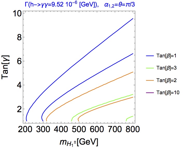
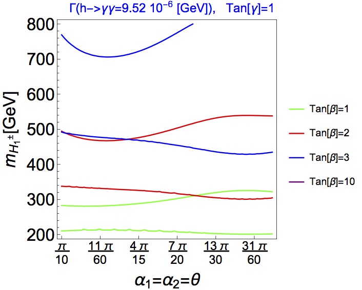
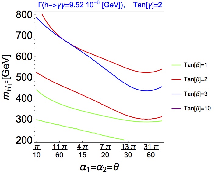
Figure 1: The contour lines show the allowed points of parameter spaces from the measurements of $h\rightarrow\gamma\gamma$ decay at the LHC in the left plane $(\tan\gamma,~{}m_{H_{1}^{\pm}})$ and center and right planes $(m_{H_{1}^{\pm}},~{}\alpha_{1,2}=\theta)$ in the Type-I 3HDM. The other parameters are fixed to be: $m_{h}=125$ GeV, $\theta_{2}=\pi/6$, $m_{H_{2}^{\pm}}=m_{H_{1}^{\pm}}+100$ GeV and $m_{12}=m_{23}=m_{13}=200$ GeV.

IV.2 $h\rightarrow Z\gamma$

In this section, we will examine the decay partial width of $h\rightarrow Z\gamma$ while respecting the parameter spaces that are not ruled out by the $\Gamma(h\rightarrow\gamma\gamma)$ analysis. Using the values of parameters in Table 3, we first focus on the decay width of $\Gamma(h\rightarrow Z\gamma)$ in the Type I 3HDM. The dependence of $\Gamma(h\rightarrow Z\gamma)$ on $m_{H_{1}^{\pm}}$ is shown on the upper panels of Fig. 2 for $\tan\gamma=1$ and different choice of $\tan\beta$. The curves show that the decay width is sensitive to the charged Higgs bosons masses. One can see that the decay width drops sharply with the charged Higgs masses $m_{H^{\pm}_{1,2}}$ increasing. The decay width is sensitive to the choice of $\tan\beta$. On the lower panel of Fig. 2, we interpret the dependence of the decay with on the CP-even mixing angles $\alpha_{1,2},~{}\theta$ for various values of $\tan\gamma$ and $m_{H_{1}^{\pm}}.$ We see that in order to have large values of $h\rightarrow Z\gamma$ small values of the CP-even mixing angles are required.

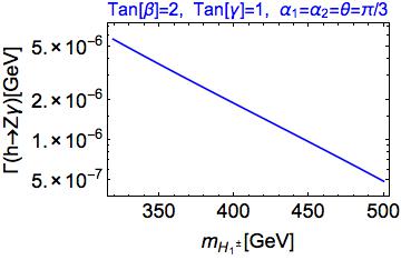
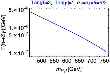
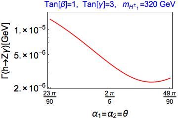
Figure 2: The decay width of $h\rightarrow Z\gamma$ as a function of $m_{H^{\pm}_{1}}$(upper panel) and $\alpha_{1,2}=\theta$ (lower panel) in the Type-I 3HDM. We take $m_{H_{2}^{\pm}}=m_{H_{1}^{\pm}}+100$ GeV, $m_{h}=125$ GeV, $m_{12}=m_{23}=m_{13}=200$ GeV, and $\theta_{2}=\pi/6.$

In Fig. 3, we present the deviation in the partial decay width of $h\rightarrow Z\gamma$ relative to the SM prediction. On the left panel range $319\leq m_{H_{1}^{\pm}}\leq 500$ is plotted, and on the right panel the range $23\pi/90\leq\alpha_{1,2}=\theta\leq 49\pi/90$ is plotted. From these plots, it is possible to see that the deviation in $\Gamma(h\rightarrow Z\gamma)$ increases with large values of $m_{H^{\pm}_{1,2}}$ and $\alpha_{1,2}=\theta$. On the right panel, the partial decay width of $h\rightarrow Z\gamma$ with respect to the SM one enhances about by a factor 2 for the case of $\tan\gamma=3$ and $\alpha_{1,2}=\theta=23\pi/90.$ As can be seen from the left panel, for $m_{H_{1}^{\pm}}=319$ GeV, the deviation from the SM prediction is about 10 % when $\tan\beta=2$ and $\tan\gamma=1$.

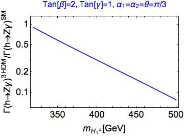
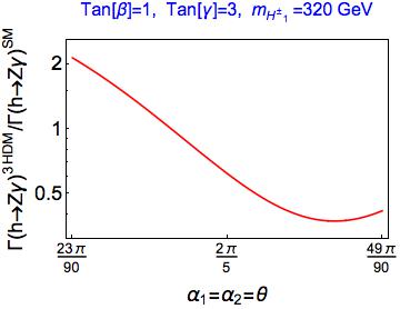
Figure 3: Dependence of $\Gamma(h\rightarrow Z\gamma)_{\text{3HDM}}/\Gamma(h\rightarrow Z\gamma)_{\text{SM}}$ on $m_{H_{1}^{\pm}}$(left panel) and $\alpha_{1,2},~{}\theta$ (right panel) in the Type-I 3HDM. We take $m_{H_{1}^{\pm}}=m_{H_{2}^{\pm}}=100$ GeV , $m_{h}=125$ GeV, $\theta_{2}=\pi/6$ and $m_{12}=m_{23}=m_{13}=200$ GeV.

To compare the branching ratio of BR$(h\rightarrow Z\gamma)$ in the Type I 3HDM to the branching ratio of BR$(h\rightarrow Z\gamma)$ in the SM, we define the ratio of two branching ratios

$$R_{\text{BR}}=\frac{BR(h\rightarrow Z\gamma)^{\text{3HDM}}}{BR(h\rightarrow Z\gamma)^{\text{SM}}},$$ (27)

where BR$(h\rightarrow Z\gamma)^{\text{SM}}$ represents the branching ratio in the SM.

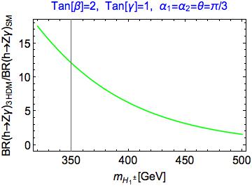
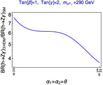
Figure 4: Dependence of $\text{BR}(h\rightarrow Z\gamma)_{\text{3HDM}}/\text{BR}(h\rightarrow Z\gamma)_{\text{SM}}$ on $m_{H_{1}^{\pm}}$ (left panel) and $\alpha_{1,2},~{}\theta$ (right panel) in the Type-I 3HDM. We take $m_{H_{1}^{\pm}}=m_{H_{2}^{\pm}}+100$ GeV, $m_{h}=125$ GeV, $\theta_{2}=\pi/6$ and $m_{12}=m_{23}=m_{13}=200$ GeV.

Fig. 4 shows the deviation in the branching ratio of BR$(h\rightarrow Z\gamma)^{\text{3HDM}}$ with respect to the SM prediction as a function of $m_{H_{1}^{\pm}}$ in the Type I-3HDM. $R_{BR}>1$ occurs due to the large contribution of the $H^{\pm}_{1,2}$ loop. The left plot in Fig. 4 presents a deviation from the SM prediction at small values of $m_{H^{\pm}_{1}}$ and $\tan\beta=2.$ The right plot in Fig. 4 appears to be compatible with the SM prediction for $\tan\beta=1,$ $\tan\gamma=3$ and the large values of $\alpha_{1,2}=\theta$. As can be seen from the left plot, BR$(h\rightarrow Z\gamma)^{\text{3HDM}}$ is close to the SM prediction at values of $m_{H_{1}^{\pm}}=500$ GeV. The current searches at the LHC have a limit of about 4 times the $h\rightarrow Z\gamma$ signal strength in the Standard Model ATLAS:2020qcv . Thus, this decay would be observed in the high-luminosity (HL) run of the LHC when $R_{BR}\simeq 1$. It is clear from the left and right plots that the enhancement of the $h\rightarrow Z\gamma$ branching ratio is so large in some regions of parameter space hence the HL-LHC could have the potential to exclude this parameter region.

Note that the ratio of two branching ratios BR$(h\rightarrow Z\gamma)^{\text{3HDM}}/\text{BR}(h\rightarrow Z\gamma)^{\text{SM}}$ is larger than that of two partial widths $\Gamma(h\rightarrow Z\gamma)^{\text{3HDM}}/\Gamma(h\rightarrow Z\gamma)^{\text{SM}}$. In the Type-I 3HDM, the total decay width is smaller than the SM prediction because the partial widths of $(h\rightarrow\bar{f}f,~{}gg)$ are significantly suppressed with respect to their SM values. As a result, there is an enhancement in the BR$(h\rightarrow Z\gamma)^{\text{3HDM}}$ relative to its SM value.

We note that we have explicitly checked that the partial decay widths of $(h\rightarrow Z\gamma(\gamma\gamma))$ in the Type-I 3HDM are nearly the same as those in the Type-Z 3HDM.

$$R_{Z\gamma(\gamma\gamma)}=\frac{\Gamma(h\rightarrow Z\gamma(\gamma\gamma))^{\text{3HDM}}}{\Gamma(h\rightarrow Z\gamma(\gamma\gamma))^{\text{SM}}},$$ (28)

where $\Gamma(h\rightarrow Z\gamma)^{\text{SM}}$ represents the partial width in the SM.

Before concluding, remarks on the correlations between the $h\rightarrow\gamma\gamma$ and $h\rightarrow Z\gamma$ partial widths in Type-I 3HDM are in order. The left panel of Fig. 5 shows the contour plot of $\Gamma^{\gamma\gamma}/\Gamma^{Z\gamma}$ in the plane of $(m_{H^{\pm}_{1}},\tan\gamma)$ with the constraint from the measurement $h\rightarrow\gamma\gamma$ decay. One can see that the allowed regions increase with large value of $\Gamma^{\gamma\gamma}/\Gamma^{Z\gamma}$. The left panel shows the regions where the partial width of $h\rightarrow Z\gamma$ could be either larger or smaller than that of $h\rightarrow\gamma\gamma$. On the right panel of Fig. 5, we discuss the correlations between $R_{\gamma\gamma}$ and $R_{Z\gamma},$ defined in Eq. (26), while we retain the decay of $h\rightarrow\gamma\gamma$ as in its measured value at the LHC. The right panel illustrates that the correlation is sensitive to the choice of $m_{H^{\pm}_{1}}$. The plots in Fig. 5 show that correlation can exist between the $h\rightarrow Z\gamma$ and $h\rightarrow\gamma\gamma$ decays at particular parameter regions. This correlation could be tested in future experiments at the LHC.

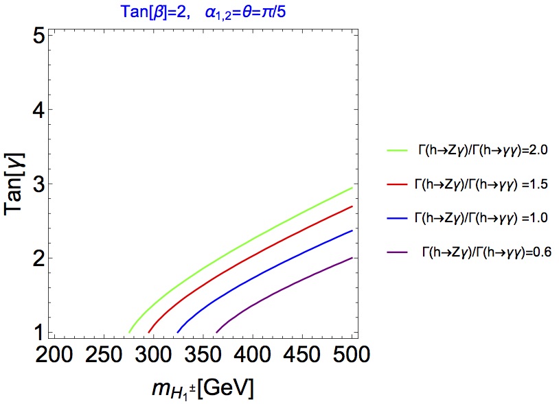
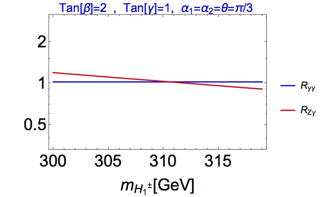
Figure 5: Left plane shows contour plot of $\Gamma^{\gamma\gamma}/\Gamma^{Z\gamma}$ as a function of $m_{H^{\pm}_{1}}$ and $\tan\gamma$ in the Type-I 3HDM. Right plane shows correlation between $R_{\gamma\gamma}$ and $R_{Z\gamma}$ in the Type-I 3HDM. We take $m_{h}=125$ GeV, $m_{H_{1}^{\pm}}=m_{H_{2}^{\pm}}+100$ GeV, $\theta_{2}=\pi/6$ and $m_{12}=m_{23}=m_{13}=200$ GeV .

IV.3 $h\rightarrow gg$

In this section, we discuss the gluonic decay widths of the 125 GeV Higgs boson $h$. First, we present the decay width $\Gamma(h\rightarrow gg)$ as a function of $\tan\beta$ for various values of $\tan\gamma$ on the left plot of Fig.6. The solid and dotted lines stand for the Type-I and Type-Z 3HDM respectively. Hence one can use them to distinguish the Type-I and Type-Z 3HDM. The decay of $h$ into $gg$ increases with $\tan\gamma$ and $\tan\beta$ in the Type-Z 3HDM, while it remains the same at large $\tan\beta$ in the Type-I 3HDM.

The right plot of Fig. 6 indicates the dependence of the CP-even mixing angles on the decay of $h$ into $gg$. The decay width is very sensitive to the change of $\alpha_{1,2}~{}\text{and}~{}\theta$. The solid and dotted lines stand for the Type-I and Type-Z 3HDM, respectively, and thus one can disentangle the two types in the gluonic decay.

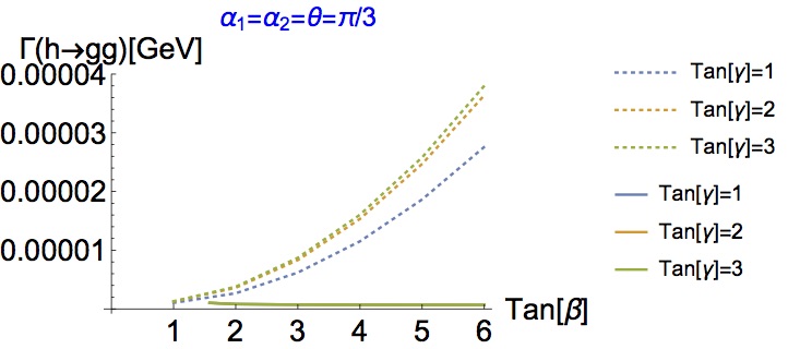
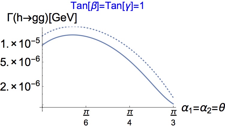
Figure 6: The left plot indicates the decay width of $h\rightarrow gg$ as a function of $\tan\beta$ in the Type-I (solid lines) and Type-Z (dotted lines) 3HDM. The right plot indicates the decay width of $h\rightarrow gg$ as a function of the CP-even mixing angles in the Type-I (solid lines) and Type-Z (dotted lines) 3HDM. We take $m_{h}=125$ GeV.

In general, some of the important parameters to distinguish different Yukawa types of the model are denoted as $\tan\beta~{}\text{and}~{}\tan\gamma.$

V CONCLUSIONS

In this work, we have analyzed the new physics contributions predicted by the 3HDM to the loop induced decays $h\rightarrow\gamma\gamma,~{}\gamma Z,~{}gg$. We have found that

• The new charged Higgs bosons $H^{\pm}_{1,2}$ can significantly alter the decay widths $h\rightarrow\gamma\gamma,~{}\gamma Z$ (where h is the lightest CP-even scalar in the 3HDM), since their loop factor is the largest among others.

• tan$\beta$, tan$\gamma$, $\alpha_{1,2},~{}\theta$, and $m_{H_{1,2}^{\pm}}$ parameters can have significant effects on these decays.

• We can disentangle the Type-I and Type-Z 3HDM only in the gluonic decays, since $\gamma\gamma$ and $Z\gamma$ decays are dominated by the $H^{\pm}_{1}$ and $H^{\pm}_{2}$ bosons loop contributions.

• $h\rightarrow Z\gamma$ branching ratio increases considerably compared to its SM value in the part of the parameter space while the $h\rightarrow\gamma\gamma$ decay is compatible with the LHC measurement. Our results on the BR$(h\rightarrow Z\gamma)$ can be tested at the LHC when $R_{BR}\simeq 1$.

• A correlation between the $h\rightarrow Z\gamma$ and $h\rightarrow\gamma\gamma$ decays exist, which could be probed in future experiments at the LHC.

In general, a large enhancement of $\Gamma(h\rightarrow Z\gamma)$ in the 3HDM may be obtained with the contributions of the new charged Higgs bosons $H^{\pm}_{1,2}$ and probed at the HL-LHC.

Appendix A Mass Matrices

Now, we determine the mass matrices in different sectors.

A.1 CP charged scalar sector

The analytic expressions for the mass matrices of the singly-charged (${\cal M}_{\pm}^{2}$) scalar states in the Higgs basis of 3HDMs can be extracted from the scalar potential as

$$V_{C}=\begin{pmatrix}w_{1}^{+}&w_{2}^{+}&w_{3}^{+}\end{pmatrix}M_{\pm}^{2}\begin{pmatrix}w_{1}^{-}\\ w_{2}^{-}\\ w_{3}^{-}\end{pmatrix}.$$ (29)

The (${\cal M}_{\pm}^{2}$) $3\times 3$ mass matrix can be diagonalized as follows:

$$(M_{C})^{2}=R^{T}\cdot M_{\pm}^{2}\cdot R=\begin{pmatrix}0&0&0\\ 0&(M_{C})^{2}_{22}&(M_{C})^{2}_{23}\\ 0&(M_{C})^{2}_{23}&(M_{C})^{2}_{33}\end{pmatrix}.$$ (30)

The matrix elements of ${\cal M}_{C}^{2}$ are given by

$$({\cal M}_{C}^{2})_{22} =-\frac{v^{2}}{2}\left[(\rho_{2}+\rho_{3})c_{\gamma}^{2}+(\kappa_{2}+\kappa_{3})s_{\gamma}^{2})\right]+m_{12}^{2}\frac{c_{\gamma}}{s_{\beta}c_{\beta}}+m_{23}^{2}\frac{s_{\gamma}}{s_{\beta}c_{\beta}},$$ (31)

$$({\cal M}_{C}^{2})_{33} =-\frac{v^{2}}{2}\left[(\rho_{2}+\rho_{3})s_{\beta}^{2}s_{\gamma}^{2}+(\sigma_{2}+\sigma_{3})c_{\beta}^{2}+(\kappa_{2}+\kappa_{3})s_{\beta}^{2}c_{\gamma}^{2}\right]$$

$$\quad+m_{12}^{2}t_{\beta}s_{\gamma}t_{\gamma}+\frac{m_{13}^{2}}{s_{\gamma}c_{\gamma}}+m_{23}^{2}\frac{t_{\beta}c_{\gamma}}{t_{\gamma}},$$ (32)

$$({\cal M}_{C}^{2})_{23} =-\frac{v^{2}}{4}(\rho_{2}+\rho_{3}-\kappa_{2}-\kappa_{3})s_{\beta}s_{2\gamma}+m_{12}^{2}\frac{s_{\gamma}}{c_{\beta}}-m_{23}^{2}\frac{c_{\gamma}}{c_{\beta}}.$$ (33)

This matrix can be fully diagonalized by employing the orthogonal matrix $O_{\theta_{2}}$ as follows:

$$O_{\theta_{2}}.(M_{C})^{2}.O_{\theta_{2}}^{T}=\begin{pmatrix}0&0&0\\ 0&m^{2}_{H^{\pm}_{1}}&0\\ 0&0&m^{2}_{H^{\pm}_{2}}\end{pmatrix}~{}~{}~{}~{}~{}~{}O_{\theta_{2}}=\begin{pmatrix}1&0&0\\ 0&\cos(\theta_{2})&-\sin(\theta_{2})\\ 0&\sin(\theta_{2})&\cos(\theta_{2})\\ \end{pmatrix}$$ (34)

Using Eqs. (A3)$-$ (A6), $\kappa_{2},\sigma_{2}~{}\text{and}~{}\rho_{2}$ can be solved as

$$\kappa_{2} =\frac{2m_{A_{1}}^{2}c_{\theta_{1}}^{2}-\frac{2m_{A_{2}}^{2}c_{\theta_{1}}s_{\theta_{1}}}{s_{\beta}t_{\gamma}}+2m_{A_{2}}^{2}s_{\theta_{1}}^{2}+\frac{m_{A_{1}}^{2}s_{2\theta_{1}}}{s_{\beta}t_{\gamma}}-4c_{\theta_{2}}^{2}m_{H_{1}{}^{\pm}}^{2}+\frac{m_{H_{2}{}^{\pm}}^{2}s_{\theta_{2}}}{c_{\gamma}s_{\beta}s_{\gamma}}-4m_{H_{2}{}^{\pm}}^{2}s_{\theta_{2}}^{2}+\frac{m_{H_{2}{}^{\pm}}^{2}s_{\theta_{2}}}{s_{\beta}t_{\gamma}}}{2v^{2}}+$$ (35)

$$\frac{-\frac{2c_{\theta_{2}}s_{\theta_{2}}t_{\gamma}\left(\frac{m_{H_{1}{}^{\pm}}^{2}}{s_{\gamma}^{2}}+\frac{m_{H_{1}{}^{\pm}}^{2}}{t_{\gamma}^{2}}+m_{H_{2}{}^{\pm}}^{2}\right)}{s_{\beta}}+\frac{m_{12}^{2}c_{\gamma}}{c_{\beta}s_{\beta}}+\frac{m_{23}^{2}s_{\gamma}}{c_{\beta}s_{\beta}}+\frac{m_{23}^{2}}{c_{\beta}s_{\beta}s_{\gamma}}-\frac{m_{12}^{2}}{c_{\beta}c_{\gamma}s_{\beta}}+\frac{m_{12}^{2}s_{\gamma}t_{\gamma}}{c_{\beta}s_{\beta}}+\frac{m_{23}^{2}c_{\gamma}}{c_{\beta}s_{\beta}t_{\gamma}}+\frac{(m_{H_{1}{{}^{\pm}}}^{2})s_{\theta_{2}}t_{\gamma}}{s_{\beta}}}{2v^{2}}$$

$$\rho_{2} =\frac{1}{2v^{2}}\left(2m_{A_{1}}^{2}c_{\theta_{1}}^{2}-4c_{\theta_{2}}^{2}m_{H_{1}{}^{\pm}}^{2}+2m_{A_{2}}^{2}s_{\theta_{1}}^{2}+\frac{m_{H_{1}{}^{\pm}}^{2}s_{\theta_{2}}}{c_{\gamma}s_{\beta}s_{\gamma}}-4m_{H_{2}{}^{\pm}}^{2}s_{\theta_{2}}^{2}+\frac{m_{H_{2}{}^{\pm}}^{2}s_{\theta_{2}}}{s_{\beta}t_{\gamma}}-\frac{m_{A_{1}}^{2}s_{2\theta_{1}}t_{\gamma}}{s_{\beta}}+\right.$$

$$\frac{m_{A_{2}}^{2}s_{2\theta_{1}}t_{\gamma}}{s_{\beta}}+\frac{m_{H_{1}{}^{\pm}}^{2}s_{\theta_{2}}t_{\gamma}}{s_{\beta}}-\frac{2c_{\theta_{2}}s_{\theta_{2}}t_{\gamma}\left(m_{H_{2}{}^{\pm}}^{2}\left(\frac{1}{s_{\gamma}^{2}}+1\right)+\frac{m_{H_{1}{}^{\pm}}^{2}}{t_{\gamma}^{2}}\right)}{s_{\beta}}+$$ (36)

$$\left.\frac{m_{12}^{2}c_{\gamma}}{c_{\beta}s_{\beta}}+\frac{m_{12}^{2}}{c_{\beta}c_{\gamma}s_{\beta}}+\frac{m_{23}^{2}s_{\gamma}}{c_{\beta}s_{\beta}}-\frac{m_{23}^{2}}{c_{\beta}s_{\beta}s_{\gamma}}+\frac{m_{12}^{2}s_{\gamma}t_{\gamma}}{c_{\beta}s_{\beta}}+\frac{m_{23}^{2}c_{\gamma}}{c_{\beta}s_{\beta}t_{\gamma}}+\frac{m_{H_{1}{}^{\pm}}^{2}s_{\theta_{2}}^{2}t_{\gamma}^{2}\left(\frac{m_{H_{1}{}^{\pm}}^{2}}{s_{\gamma}^{2}}+\frac{m_{H_{1}{}^{\pm}}^{2}}{t_{\gamma}^{2}}+m_{H_{2}{}^{\pm}}^{2}\right)}{s_{\beta}^{2}}\right)$$

$$\sigma_{2} =\frac{1}{4v^{2}}\left(\frac{\left(m_{A_{1}}^{2}-m_{A_{2}}^{2}\right)\left(c_{2\beta}-3\right)c_{\theta_{1}}^{2}}{c_{\beta}^{2}}-\frac{2\left(m_{A_{1}}^{2}-m_{A_{2}}^{2}\right)c_{2\gamma}s_{2\theta_{1}}t_{\beta}}{c_{\beta}c_{\gamma}s_{\gamma}}+\frac{4c_{2\gamma}\left(m_{H_{1}{}^{\pm}}^{2}-m_{H_{2}{{}^{\pm}}}^{2}\right)s_{\theta_{2}}t_{\beta}}{c_{\beta}c_{\gamma}s_{\gamma}}+\right.$$

$$\left(t_{\beta}^{2}-1\right)\left(\left(m_{A_{1}}^{2}-m_{A_{2}}^{2}\right)s_{\theta_{1}}^{2}-m_{A_{1}}^{2}-m_{A_{2}}^{2}+c_{2\theta}\left(m_{H_{1}{}^{\pm}}^{2}-m_{H_{2}{}^{\pm}}^{2}\right)+m_{H_{1}{}^{\pm}}^{2}+3m_{H_{2}{}^{\pm}}^{2}\right)+$$ (37)

$$\frac{3m_{A_{1}}^{2}s_{\theta_{1}}^{2}+m_{A_{1}}^{2}+m_{A_{2}}^{2}-2\left(c_{2\beta}-3\right)c_{\theta_{2}}^{2}\left(m_{H_{1}{}^{\pm}}^{2}-m_{H_{2}{}^{\pm}}^{2}\right)-2m_{H_{1}{}^{\pm}}^{2}-2m_{H_{2}{}^{\pm}}^{2}}{c_{\beta}^{2}}$$

$$\frac{3m_{A_{2}}^{2}s_{\theta_{1}}^{2}-\frac{4m_{13}^{2}}{c_{\gamma}s_{\gamma}}-6s_{\theta_{2}}^{2}m_{H_{1}{}^{\pm}}^{2}+6s_{\theta_{2}}^{2}m_{H_{2}{}^{\pm}}^{2}+m_{13}^{2}s_{2\gamma}+2m_{13}^{2}s_{\gamma}^{2}t_{\gamma}+6m_{13}^{2}t_{\gamma}+\frac{8m_{13}^{2}}{t_{\gamma}}}{c_{\beta}^{2}}\Biggr{)}.$$

A.2 CP odd scalar sector

The analytic expressions for the mass matrices of the CP-odd scalars $({\cal M}_{P}^{2})$ in the Higgs basis of 3HDM can be extracted from the scalar potential as

$$V_{C}=\begin{pmatrix}z_{1}&z_{2}&z_{3}\end{pmatrix}\frac{M_{P}^{2}}{2}\begin{pmatrix}z_{1}\\ z_{2}\\ z_{3}\end{pmatrix}.$$ (38)

The CP-odd scalar mass matrix ${\cal M}_{P}^{2}$ can be diagonalized as follows:

$$(M_{A})^{2}=R^{T}\cdot M_{P}^{2}\cdot R=\begin{pmatrix}0&0&0\\ 0&(M_{A})^{2}_{22}&(M_{A})^{2}_{23}\\ 0&(M_{A})^{2}_{23}&(M_{A})^{2}_{33}\end{pmatrix}.$$

The matrix elements of ${\cal M}_{A}^{2}$ is given by

$$({\cal M}_{A}^{2})_{22} =-v^{2}\left(\rho_{3}c_{\gamma}^{2}+\kappa_{3}s_{\gamma}^{2}\right)+m_{13}^{2}\frac{c_{\gamma}}{s_{\beta}c_{\beta}}+m_{23}^{2}\frac{s_{\gamma}}{s_{\beta}c_{\beta}},$$ (39)

$$({\cal M}_{A}^{2})_{33} =-v^{2}\left(\rho_{3}s_{\beta}^{2}s_{\gamma}^{2}+\sigma_{3}c_{\beta}^{2}+\kappa_{3}s_{\beta}^{2}c_{\gamma}^{2}\right)+m_{12}^{2}t_{\beta}s_{\gamma}t_{\gamma}+m_{13}^{2}\frac{s_{\gamma}}{s_{\gamma}c_{\gamma}}+m_{23}^{2}\frac{t_{\beta}c_{\gamma}}{t_{\gamma}},$$ (40)

$$({\cal M}_{A}^{2})_{23} =-\frac{v^{2}}{2}(\rho_{3}-\kappa_{3})s_{\beta}s_{2\gamma}+m_{12}^{2}\frac{s_{\gamma}}{c_{\beta}}-m_{23}^{2}\frac{c_{\gamma}}{c_{\beta}}.$$ (41)

In order to fully diagonalise this matrix, an orthogonal matrix $O_{\theta_{1}}$ can be employed as

$$O_{\theta_{1}}.(M_{A})^{2}.O_{\theta_{1}}^{T}=\begin{pmatrix}0&0&0\\ 0&m^{2}_{A_{1}}&0\\ 0&0&m^{2}_{A_{2}}\end{pmatrix}~{}~{}~{}~{}~{}~{}O_{\theta_{1}}=\begin{pmatrix}1&0&0\\ 0&\cos(\theta_{1})&-\sin(\theta_{1})\\ 0&\sin(\theta_{1})&\cos(\theta_{1})\\ \end{pmatrix}.$$ (42)

Using Eqs. (A11)$-$(A14), $\kappa_{3},\sigma_{3}~{}\text{and}~{}\rho_{3}$ can be solved as

$$\kappa_{3}= \frac{-2m_{A_{1}}^{2}c_{\theta_{1}}^{2}+\frac{2\left(m_{A_{2}}^{2}-m_{A_{1}}^{2}\right)c_{\theta_{1}}s_{\theta_{1}}}{s_{\beta}t_{\gamma}}-2m_{A_{2}}^{2}s_{\theta_{1}}^{2}+\frac{m_{23}^{2}s_{\gamma}}{c_{\beta}s_{\beta}}+\frac{m_{23}^{2}}{c_{\beta}s_{\beta}s_{\gamma}}-\frac{m_{12}^{2}}{c_{\beta}c_{\gamma}s_{\beta}}+\frac{m_{12}^{2}s_{\gamma}t_{\gamma}}{c_{\beta}s_{\beta}}+\frac{m_{23}^{2}c_{\gamma}+m_{12}^{2}s_{\gamma}}{c_{\beta}s_{\beta}t_{\gamma}}}{2v^{2}}$$ (43)

$$\rho_{3}= \frac{-2m_{A_{1}}^{2}c_{\theta_{1}}^{2}-2m_{A_{2}}^{2}s_{\theta_{1}}^{2}+\frac{\left(m_{A_{1}}^{2}-m_{A_{2}}^{2}\right)s_{2\theta_{1}}t_{\gamma}}{s_{\beta}}+\frac{m_{12}^{2}}{c_{\beta}c_{\gamma}s_{\beta}}+\frac{m_{23}^{2}s_{\gamma}}{c_{\beta}s_{\beta}}-\frac{m_{23}^{2}}{c_{\beta}s_{\beta}s_{\gamma}}+\frac{m_{12}^{2}s_{\gamma}t_{\gamma}}{c_{\beta}s_{\beta}}+\frac{m_{23}^{2}c_{\gamma}+m_{12}^{2}s_{\gamma}}{c_{\beta}s_{\beta}t_{\gamma}}}{2v^{2}}$$ (44)

$$\sigma_{3}= -\frac{\frac{c_{2\beta}\left(\left(m_{A_{1}}^{2}-m_{A_{2}}^{2}\right)c_{2\theta_{1}}+m_{A_{1}}^{2}+m_{A_{2}}^{2}\right)-3\left(m_{A_{1}}^{2}-m_{A_{2}}^{2}\right)c_{\theta_{1}}^{2}+3m_{A_{1}}^{2}s_{\theta_{1}}^{2}-3m_{A_{2}}^{2}s_{\theta_{1}}^{2}+m_{A_{1}}^{2}+m_{A_{2}}^{2}-\frac{4m_{13}^{2}}{c_{\gamma}s_{\gamma}}}{c_{\beta}}+\frac{2\left(m_{A_{2}}^{2}-m_{A_{1}}^{2}\right)c_{2\gamma}s_{2\theta_{1}}t_{\beta}}{c_{\gamma}s_{\gamma}}}{4v^{2}c_{\beta}}$$ (45)

A.3 CP even scalar sector

In the general weak basis, the CP-even scalar mass matrix $M^{2}_{H}$ can be extracted from the potential as

$$V_{S}=\begin{pmatrix}h_{1}&h_{2}&h_{3}\end{pmatrix}\frac{M_{H}^{2}}{2}\begin{pmatrix}h_{1}\\ h_{2}\\ h_{3}\end{pmatrix}.$$ (46)

The matrix elements of ${\cal M}_{H}^{2}$ are given by

$$({\cal M}_{H}^{2})_{11} =\frac{m_{12}^{2}t_{\beta}}{c_{\gamma}}+\lambda_{1}v^{2}c_{\beta}^{2}c_{\gamma}^{2}+m_{13}^{2}t_{\gamma},$$ (47)

$$({\cal M}_{H}^{2})_{22} =\frac{m_{12}^{2}c_{\gamma}}{t_{\beta}}+\frac{m_{23}^{2}s_{\gamma}}{t_{\beta}}+\lambda_{2}v^{2}s_{\beta}^{2},$$ (48)

$$({\cal M}_{H}^{2})_{33} =\lambda_{3}v^{2}c_{\beta}^{2}s_{\gamma}^{2}+\frac{m_{23}^{2}t_{\beta}}{s_{\gamma}}+\frac{m_{13}^{2}}{t_{\gamma}},$$ (49)

$$({\cal M}_{H}^{2})_{12} =\left(\rho_{1}+\rho_{2}+\rho_{3}\right)v^{2}c_{\beta}c_{\gamma}s_{\beta}-m_{12}^{2},$$ (50)

$$({\cal M}_{H}^{2})_{13} =\left(\sigma_{1}+\sigma_{2}+\sigma_{3}\right)v^{2}c_{\beta}^{2}c_{\gamma}s_{\gamma}-m_{13}^{2},$$ (51)

$$({\cal M}_{H}^{2})_{23} =\left(\kappa_{1}+\kappa_{2}+\kappa_{3}\right)v^{2}c_{\beta}s_{\beta}s_{\gamma}-m_{23}^{2}.$$ (52)

In the above expressions, we used the shorthand notations $c_{X}=\cos X$, $s_{X}=\sin X$ and $t_{X}=\tan X$.

For the masses of the three neutral physical states, $h,$ $H_{1}$ and $H_{2}$, we need to diagonalise the $3\times 3$ mass matrix $M^{2}_{H}$, defined in the general weak basis, by employing the orthogonal matrix $O$ given in Eq. (13) as

$$O^{T}\cdot M_{H}^{2}\cdot O=\begin{pmatrix}m_{h}^{2}&0&0\\ 0&m_{H_{1}}^{2}&0\\ 0&0&m_{H_{2}}^{2}\end{pmatrix}.$$ (53)

Finally, the remaining parameters $\lambda_{1},~{}\lambda_{2},~{}\lambda_{3},~{}\kappa_{1},\sigma_{1}~{}\text{and}~{}\rho_{1}$ can be obtained from Eqs. (A19)$-$(A25) as follows:

$$\lambda_{1} =-\frac{c_{\alpha_{1}}^{2}\left(-\left(c_{\alpha_{2}}^{2}m_{h}^{2}+m_{H_{1}}^{2}s_{\alpha_{2}}^{2}\right)\right)+\frac{m_{12}^{2}t_{\beta}}{c_{\gamma}}-m_{H_{2}}^{2}s_{\alpha_{1}}^{2}+m_{13}^{2}t_{\gamma}}{v^{2}c_{\beta}^{2}c_{\gamma}^{2}}$$ (54)

$$\lambda_{2} =\frac{c_{\alpha_{2}}^{2}\left(c_{\theta}^{2}m_{H_{1}}^{2}+m_{h}^{2}s_{\alpha_{1}}^{2}s_{\theta}^{2}\right)-c_{\alpha_{2}}s_{\alpha_{1}}s_{\alpha_{2}}s_{2\theta}\left(m_{h}^{2}-m_{H_{1}}^{2}\right)+c_{\alpha_{1}}^{2}m_{H_{2}}^{2}s_{\theta}^{2}}{v^{2}s_{\beta}^{2}}+$$ (55)

$$\frac{c_{\theta}^{2}m_{h}^{2}s_{\alpha_{2}}^{2}-\frac{m_{12}^{2}c_{\gamma}}{t_{\beta}}+m_{H_{1}}^{2}s_{\alpha_{1}}^{2}s_{\alpha_{2}}^{2}s_{\theta}^{2}-\frac{m_{23}^{2}s_{\gamma}}{t_{\beta}}}{v^{2}s_{\beta}^{2}}$$

$$\lambda_{3} =\frac{-c_{\alpha_{2}}^{2}c_{\theta}^{2}m_{h}^{2}s_{\alpha_{1}}^{2}-2c_{\alpha_{2}}c_{\theta}m_{h}^{2}s_{\alpha_{1}}s_{\alpha_{2}}s_{\theta}+c_{\alpha_{1}}^{2}\left(-c_{\theta}^{2}\right)m_{H_{2}}^{2}-c_{\alpha_{2}}^{2}m_{H_{1}}^{2}s_{\theta}^{2}}{v^{2}c_{\beta}^{2}s_{\gamma}^{2}}+$$ (56)

$$-\frac{-c_{\theta}^{2}m_{H_{1}}^{2}s_{\alpha_{1}}^{2}s_{\alpha_{2}}^{2}+2c_{\alpha_{2}}c_{\theta}m_{H_{1}}^{2}s_{\alpha_{1}}s_{\alpha_{2}}s_{\theta}-m_{h}^{2}s_{\alpha_{2}}^{2}s_{\theta}^{2}+\frac{m_{23}^{2}t_{\beta}}{s_{\gamma}}+\frac{m_{13}^{2}}{t_{\gamma}}}{v^{2}c_{\beta}^{2}s_{\gamma}^{2}}$$

$$\kappa_{1} =\frac{1}{2v^{2}s_{\gamma}}\left(4c_{\theta_{2}}^{2}m_{H_{1}{}^{\pm}}^{2}s_{\gamma}-\frac{2c_{\alpha_{1}}^{2}c_{\theta}m_{H_{2}}^{2}s_{\theta}}{c_{\beta}s_{\beta}}+\frac{c_{\alpha_{2}}^{2}s_{2\theta}\left(c_{2\alpha_{1}}m_{h}^{2}-m_{h}^{2}+2m_{H_{1}}^{2}\right)}{2c_{\beta}s_{\beta}}-\right.$$ (57)

$$\frac{c_{\alpha_{2}}s_{\alpha_{1}}s_{\alpha_{2}}\left(c_{2\theta}\left(m_{H_{1}}^{2}-m_{h}^{2}\right)+m_{h}^{2}+m_{H_{1}}^{2}\right)}{c_{\beta}s_{\beta}}+\frac{m_{h}^{2}s_{\alpha_{2}}^{2}s_{2\theta}}{c_{\beta}s_{\beta}}-\frac{2c_{\theta}m_{H_{1}}^{2}s_{\alpha_{1}}^{2}s_{\alpha_{2}}^{2}s_{\theta}}{c_{\beta}s_{\beta}}+\frac{c_{\theta}^{2}m_{h}^{2}s_{\alpha_{1}}s_{2\alpha_{2}}}{c_{\beta}s_{\beta}}+$$

$$\frac{m_{H_{1}}^{2}s_{\alpha_{1}}s_{2\alpha_{2}}s_{\theta}^{2}}{c_{\beta}s_{\beta}}+\frac{m_{H_{1}{}^{\pm}}^{2}s_{\theta_{2}}}{c_{\gamma}s_{\beta}}-\frac{m_{H_{2}{}^{\pm}}^{2}s_{\theta_{2}}}{c_{\gamma}s_{\beta}}+4m_{H_{2}{}^{\pm}}^{2}s_{\gamma}s_{\theta_{2}}^{2}-\frac{m_{H_{1}{}^{\pm}}^{2}s_{\gamma}s_{\theta_{2}}t_{\gamma}}{s_{\beta}}+$$

$$\left.\frac{c_{\gamma}\left(\left(m_{H_{1}{}^{\pm}}^{2}-m_{H_{2}{}^{\pm}}^{2}\right)s_{\theta_{2}}-\frac{2m_{12}^{2}s_{\gamma}}{c_{\beta}}\right)}{s_{\beta}}-\frac{2m_{23}^{2}c_{\gamma}^{2}}{c_{\beta}s_{\beta}}-\frac{2m_{23}^{2}s_{\gamma}^{2}}{c_{\beta}s_{\beta}}+\frac{2m_{12}^{2}t_{\gamma}}{c_{\beta}s_{\beta}}-\frac{2m_{12}^{2}s_{\gamma}^{2}t_{\gamma}}{c_{\beta}s_{\beta}}+\frac{m_{H_{2}{}^{\pm}}^{2}s_{\gamma}s_{\theta_{2}}t_{\gamma}}{s_{\beta}}\right)$$

$$\rho_{1}=\frac{1}{2v^{2}}\left(4c_{\theta_{2}}^{2}m_{H_{1}{}^{\pm}}^{2}-\frac{2c_{\alpha_{1}}c_{\alpha_{2}}^{2}m_{h}^{2}s_{\alpha_{1}}s_{\theta}}{c_{\beta}c_{\gamma}s_{\beta}}+\frac{m_{H_{2}}^{2}s_{2\alpha_{1}}s_{\theta}}{c_{\beta}c_{\gamma}s_{\beta}}-\frac{2c_{\alpha_{1}}c_{\alpha_{2}}c_{\theta}m_{H_{1}}^{2}s_{\alpha_{2}}}{c_{\beta}c_{\gamma}s_{\beta}}-\frac{2c_{\alpha_{1}}m_{H_{1}}^{2}s_{\alpha_{1}}s_{\alpha_{2}}^{2}s_{\theta}}{c_{\beta}c_{\gamma}s_{\beta}}+\right.$$ (58)

$$\frac{c_{\alpha_{1}}c_{\theta}m_{h}^{2}s_{2\alpha_{2}}}{c_{\beta}c_{\gamma}s_{\beta}}-\frac{m_{H_{1}{}^{\pm}}^{2}s_{\theta_{2}}}{c_{\gamma}s_{\beta}s_{\gamma}}+\frac{m_{H_{2}{}^{\pm}}^{2}s_{\theta_{2}}}{c_{\gamma}s_{\beta}s_{\gamma}}+4m_{H_{2}{}^{\pm}}^{2}s_{\theta_{2}}^{2}+\frac{m_{H_{1}{}^{\pm}}^{2}s_{\theta_{2}}}{s_{\beta}t_{\gamma}}-\frac{m_{H_{2}{}^{\pm}}^{2}s_{\theta_{2}}}{s_{\beta}t_{\gamma}}-$$

$$\left.\frac{2m_{23}^{2}}{c_{\beta}s_{\beta}s_{\gamma}}-\frac{2m_{23}^{2}s_{\gamma}}{c_{\beta}s_{\beta}}-\frac{2m_{12}^{2}s_{\gamma}t_{\gamma}}{c_{\beta}s_{\beta}}-\frac{2\left(m_{23}^{2}c_{\gamma}+m_{12}^{2}s_{\gamma}\right)}{c_{\beta}s_{\beta}t_{\gamma}}+\frac{m_{\left(H_{1}\right){}^{+}}^{2}s_{\theta_{2}}t_{\gamma}}{s_{\beta}}+\frac{m_{\left(H_{2}\right){}^{+}}^{2}s_{\theta_{2}}t_{\gamma}}{s_{\beta}}\right)$$

$$\sigma_{1} =\frac{1}{8v^{2}c_{\beta}}\left(\frac{6\left(c_{2\beta}-2\right)c_{\theta_{2}}^{2}\left(m_{H_{1}{}^{\pm}}^{2}-m_{H_{2}{}^{\pm}}^{2}\right)}{c_{\beta}}-\frac{8c_{2\gamma}\left(m_{H_{1}{}^{\pm}}^{2}-m_{H_{2}{}^{\pm}}^{2}\right)s_{\theta_{2}}t_{\beta}}{c_{\gamma}s_{\gamma}}-\right.$$ (59)

$$\frac{1}{c_{\beta}c_{\gamma}s_{\gamma}}\left(-c_{\gamma}s_{\gamma}\left(c_{2\beta}\left(c_{2\theta}\left(m_{H_{1}{}^{\pm}}^{2}-m_{H_{2}{}^{\pm}}^{2}\right)+m_{\left(H_{1}\right){}^{+}}^{2}+7m_{H_{2}{}^{\pm}}^{2}\right)+4\left(m_{\left(H_{1}\right){}^{+}}^{2}+m_{H_{2}{}^{\pm}}^{2}\right)\right)+\right.$$

$$8c_{\alpha_{1}}\left(c_{\alpha_{2}}s_{\alpha_{2}}s_{\theta}\left(m_{H_{1}}^{2}-m_{h}^{2}\right)+c_{\theta}s_{\alpha_{1}}\left(-c_{\alpha_{2}}^{2}m_{h}^{2}-m_{H_{1}}^{2}s_{\alpha_{2}}^{2}+m_{H_{2}}^{2}\right)\right)-6m_{H_{1}{}^{\pm}}^{2}s_{2\gamma}s_{\theta_{2}}^{2}+$$

$$\left.\left.16m_{13}^{2}c_{\gamma}^{2}+6m_{H_{2}{}^{\pm}}^{2}s_{2\gamma}s_{\theta_{2}}^{2}-8m_{13}^{2}+4m_{13}^{2}s_{\gamma}^{4}+12m_{13}^{2}s_{\gamma}^{2}+m_{13}^{2}s_{2\gamma}^{2}\right)\right)$$

Appendix B Coefficients of $hH^{+}_{i}H^{-}_{i}$ Terms in the Potential

The coefficients of triple scalar couplings in the potential are explicitly given as

$$a= \frac{-1}{2v}\left(c_{\alpha_{1}}c_{\alpha_{2}}s_{\beta}\left(c_{\alpha_{1}}c_{\theta}s_{2\alpha_{2}}-c_{\alpha_{2}}^{2}s_{2\alpha_{1}}s_{\theta}\right)\left(\frac{c_{\theta_{2}}}{t_{\beta}}+s_{\gamma}s_{\theta_{2}}\right){}^{2}-\right.$$ (60)

$$s_{\beta}\left(c_{\alpha_{2}}c_{\theta}s_{\alpha_{1}}+s_{\alpha_{2}}s_{\theta}\right)\left(c_{\alpha_{2}}^{2}s_{\alpha_{1}}^{2}s_{2\theta}-c_{2\theta}s_{2\alpha_{2}}s_{\alpha_{1}}-s_{\alpha_{2}}^{2}s_{2\theta}\right)\left(\frac{c_{\theta_{2}}}{t_{\beta}}+s_{\gamma}s_{\theta_{2}}\right){}^{2}-$$

$$2s_{\beta}\left(c_{\alpha_{2}}s_{\alpha_{1}}s_{\theta}-c_{\theta}s_{\alpha_{2}}\right)\left(c_{\alpha_{2}}^{2}s_{\alpha_{1}}^{2}s_{\theta}^{2}+c_{\theta}\left(c_{\theta}s_{\alpha_{2}}^{2}-s_{\alpha_{1}}s_{2\alpha_{2}}s_{\theta}\right)\right)\left(\frac{c_{\theta_{2}}}{t_{\beta}}+s_{\gamma}s_{\theta_{2}}\right){}^{2}+$$

$$2c_{\alpha_{1}}^{3}c_{\alpha_{2}}^{3}c_{\gamma}s_{\beta}t_{\beta}+c_{\gamma}s_{\beta}t_{\beta}\left(c_{\alpha_{2}}s_{\alpha_{1}}s_{\theta}-c_{\theta}s_{\alpha_{2}}\right)\left(c_{\alpha_{2}}^{2}s_{2\alpha_{1}}s_{\theta}-c_{\alpha_{1}}c_{\theta}s_{2\alpha_{2}}\right)+$$

$$c_{\gamma}s_{\beta}t_{\beta}\left(c_{\alpha_{2}}c_{\theta}s_{\alpha_{1}}+s_{\alpha_{2}}s_{\theta}\right)\left(c_{\alpha_{2}}^{2}c_{\theta}s_{2\alpha_{1}}+c_{\alpha_{1}}s_{2\alpha_{2}}s_{\theta}\right)+\frac{c_{\alpha_{1}}c_{\alpha_{2}}c_{\beta}\left(c_{\alpha_{2}}^{2}c_{\theta}s_{2\alpha_{1}}+c_{\alpha_{1}}s_{2\alpha_{2}}s_{\theta}\right)\left(s_{\theta_{2}}-c_{\theta_{2}}s_{\gamma}t_{\beta}\right){}^{2}}{s_{\gamma}}+$$

$$\frac{c_{\beta}\left(c_{\alpha_{2}}s_{\alpha_{1}}s_{\theta}-c_{\theta}s_{\alpha_{2}}\right)\left(c_{\alpha_{2}}^{2}s_{\alpha_{1}}^{2}s_{2\theta}-c_{2\theta}s_{2\alpha_{2}}s_{\alpha_{1}}-s_{\alpha_{2}}^{2}s_{2\theta}\right)\left(s_{\theta_{2}}-c_{\theta_{2}}s_{\gamma}t_{\beta}\right){}^{2}}{s_{\gamma}}+$$

$$\left.\frac{2c_{\beta}\left(c_{\alpha_{2}}c_{\theta}s_{\alpha_{1}}+s_{\alpha_{2}}s_{\theta}\right)\left(c_{\alpha_{2}}^{2}c_{\theta}^{2}s_{\alpha_{1}}^{2}+c_{\theta}s_{2\alpha_{2}}s_{\alpha_{1}}s_{\theta}+s_{\alpha_{2}}^{2}s_{\theta}^{2}\right)\left(s_{\theta_{2}}-c_{\theta_{2}}s_{\gamma}t_{\beta}\right){}^{2}}{s_{\gamma}}\right)$$

$$b= \frac{1}{4v}\left(-\frac{4\left(c_{\alpha_{2}}c_{\theta}s_{\alpha_{1}}+s_{\alpha_{2}}s_{\theta}\right)\left(c_{\beta}c_{\theta_{2}}+s_{\beta}s_{\gamma}s_{\theta_{2}}\right){}^{2}\left(2c_{\theta_{2}}^{2}s_{\beta}s_{\gamma}+c_{\gamma}s_{2\theta_{2}}\right)}{t_{\beta}}+\right.$$ (61)

$$c_{\gamma}^{2}s_{\beta}^{2}\left(c_{\alpha_{2}}c_{\theta}s_{\alpha_{1}}+s_{\alpha_{2}}s_{\theta}\right)\left(\frac{4c_{2\gamma}s_{2\theta_{2}}t_{\beta}}{c_{\gamma}}-\frac{2s_{\gamma}\left(\left(2c_{2\beta}-3\right)c_{\theta_{2}}^{2}+3s_{\theta_{2}}^{2}+1\right)}{c_{\beta}}\right)+$$

$$c_{\gamma}s_{\beta}\left(c_{\gamma}\left(c_{\alpha_{2}}c_{\theta}s_{\alpha_{1}}+s_{\alpha_{2}}s_{\theta}\right)+c_{\alpha_{1}}c_{\alpha_{2}}s_{\gamma}\right)\left(c_{\beta}s_{\theta_{2}}-c_{\theta_{2}}s_{\beta}s_{\gamma}\right)\left(\frac{\left(6-4c_{2\beta}\right)c_{\theta_{2}}^{2}+3c_{2\theta_{2}}-5}{c_{\beta}}+\frac{4c_{2\gamma}s_{2\theta_{2}}t_{\beta}}{c_{\gamma}s_{\gamma}}\right)+$$

$$4\left(c_{\alpha_{2}}s_{\alpha_{1}}s_{\theta}-c_{\theta}s_{\alpha_{2}}\right)\left(c_{\theta_{2}}s_{\beta}s_{\gamma}-c_{\beta}s_{\theta_{2}}\right){}^{2}\left(2c_{\theta_{2}}^{2}s_{\beta}+\frac{s_{2\theta_{2}}}{t_{\gamma}}\right)+4\left(c_{\beta}s_{\gamma}\left(c_{\theta}s_{\alpha_{2}}-c_{\alpha_{2}}s_{\alpha_{1}}s_{\theta}\right)+\right.$$

$$\left.+s_{\beta}\left(c_{\alpha_{2}}c_{\theta}s_{\alpha_{1}}+s_{\alpha_{2}}s_{\theta}\right)\right)(c_{\beta}s_{\theta_{2}}-c_{\theta_{2}}s_{\beta}s_{\gamma})\left(c_{\beta}c_{\theta_{2}}+s_{\beta}s_{\gamma}s_{\theta_{2}}\right)\left(2c_{\theta_{2}}^{2}+\frac{s_{2\theta_{2}}}{s_{\beta}t_{\gamma}}\right)+$$

$$\frac{c_{\alpha_{1}}c_{\alpha_{2}}\left(c_{\theta_{2}}s_{\beta}s_{\gamma}-c_{\beta}s_{\theta_{2}}\right){}^{2}\left(\frac{4c_{2\gamma}s_{2\theta_{2}}t_{\beta}}{c_{\gamma}}-\frac{2s_{\gamma}\left(\left(2c_{2\beta}-3\right)c_{\theta_{2}}^{2}+3s_{\theta_{2}}^{2}+1\right)}{c_{\beta}}\right)}{t_{\gamma}}+$$

$$4c_{\gamma}^{2}s_{\beta}^{2}\left(c_{\alpha_{2}}s_{\alpha_{1}}s_{\theta}-c_{\theta}s_{\alpha_{2}}\right)\left(2c_{\theta_{2}}^{2}s_{\beta}-s_{2\theta_{2}}t_{\gamma}\right)-\frac{4c_{\alpha_{1}}c_{\alpha_{2}}c_{\gamma}\left(c_{\beta}c_{\theta_{2}}+s_{\beta}s_{\gamma}s_{\theta_{2}}\right){}^{2}\left(2c_{\theta_{2}}^{2}s_{\beta}-s_{2\theta_{2}}t_{\gamma}\right)}{t_{\beta}}+$$

$$\left.c_{\gamma}s_{\beta}\left(c_{\beta}c_{\theta_{2}}+s_{\beta}s_{\gamma}s_{\theta_{2}}\right)\left(c_{\beta}c_{\gamma}\left(c_{\theta}s_{\alpha_{2}}-c_{\alpha_{2}}s_{\alpha_{1}}s_{\theta}\right)+c_{\alpha_{1}}c_{\alpha_{2}}s_{\beta}\right)\left(-8c_{\theta_{2}}^{2}-\frac{4c_{\theta_{2}}s_{\theta_{2}}}{s_{\beta}t_{\gamma}}+\frac{2s_{2\theta_{2}}\left(\frac{1}{c_{\gamma}s_{\gamma}}+t_{\gamma}\right)}{s_{\beta}}\right)\right)$$

$$c= \frac{1}{8v}\left(-\frac{8\left(c_{\alpha_{2}}c_{\theta}s_{\alpha_{1}}+s_{\alpha_{2}}s_{\theta}\right)\left(c_{\beta}c_{\theta_{2}}+s_{\beta}s_{\gamma}s_{\theta_{2}}\right){}^{2}\left(2s_{\beta}s_{\gamma}s_{\theta_{2}}^{2}-c_{\gamma}s_{2\theta_{2}}\right)}{t_{\beta}}+\right.$$ (62)

$$2c_{\gamma}^{2}s_{\beta}^{2}\left(c_{\alpha_{2}}c_{\theta}s_{\alpha_{1}}+s_{\alpha_{2}}s_{\theta}\right)\left(-\frac{s_{\gamma}\left(6c_{\theta_{2}}^{2}+\left(4c_{2\beta}-6\right)s_{\theta_{2}}^{2}+2\right)}{c_{\beta}}-\frac{4c_{2\gamma}s_{2\theta_{2}}t_{\beta}}{c_{\gamma}}\right)+$$

$$c_{\gamma}s_{\beta}\left(c_{\gamma}\left(c_{\alpha_{2}}c_{\theta}s_{\alpha_{1}}+s_{\alpha_{2}}s_{\theta}\right)+c_{\alpha_{1}}c_{\alpha_{2}}s_{\gamma}\right)(c_{\beta}s_{\theta_{2}}-c_{\theta_{2}}s_{\beta}s_{\gamma})\left(\frac{2\left(c_{\beta-\theta_{2}}+c_{\beta+\theta_{2}}-2c_{2\beta}-6c_{2\theta_{2}}-2\right)}{c_{\beta}}-\right.$$

$$\left.\frac{8c_{2\gamma}s_{2\theta_{2}}t_{\beta}}{c_{\gamma}s_{\gamma}}\right)+8\left(c_{\alpha_{2}}s_{\alpha_{1}}s_{\theta}-c_{\theta}s_{\alpha_{2}}\right)\left(c_{\theta_{2}}s_{\beta}s_{\gamma}-c_{\beta}s_{\theta_{2}}\right){}^{2}\left(2s_{\beta}s_{\theta_{2}}^{2}-\frac{s_{2\theta_{2}}}{t_{\gamma}}\right)+$$

$$4s_{\beta}^{2}\left(c_{\alpha_{2}}s_{\alpha_{1}}s_{\theta}-c_{\theta}s_{\alpha_{2}}\right)\left(c_{\gamma}s_{\gamma}s_{2\theta_{2}}+c_{\gamma}^{2}\left(4s_{\beta}s_{\theta_{2}}^{2}-\frac{s_{2\theta_{2}}}{t_{\gamma}}\right)+\frac{s_{2\theta_{2}}}{t_{\gamma}}\right)+$$

$$\frac{2c_{\alpha_{1}}c_{\alpha_{2}}\left(c_{\theta_{2}}s_{\beta}s_{\gamma}-c_{\beta}s_{\theta_{2}}\right){}^{2}\left(-\frac{s_{\gamma}\left(6c_{\theta_{2}}^{2}+\left(4c_{2\beta}-6\right)s_{\theta_{2}}^{2}+2\right)}{c_{\beta}}-\frac{4c_{2\gamma}s_{2\theta_{2}}t_{\beta}}{c_{\gamma}}\right)}{t_{\gamma}}-$$

$$2\left(c_{\beta}s_{\gamma}\left(c_{\theta}s_{\alpha_{2}}-c_{\alpha_{2}}s_{\alpha_{1}}s_{\theta}\right)+\right.\left.s_{\beta}\left(c_{\alpha_{2}}c_{\theta}s_{\alpha_{1}}+s_{\alpha_{2}}s_{\theta}\right)\right)(c_{\beta}s_{\theta_{2}}-c_{\theta_{2}}s_{\beta}s_{\gamma})(c_{\beta}c_{\theta_{2}}+s_{\beta}s_{\gamma}s_{\theta_{2}})$$

$$\left(-8s_{\theta_{2}}^{2}+\frac{2s_{2\theta_{2}}\left(\frac{1}{c_{\gamma}s_{\gamma}}+\frac{1}{t_{\gamma}}\right)}{s_{\beta}}-\frac{4c_{\theta_{2}}s_{\theta_{2}}t_{\gamma}}{s_{\beta}}\right)+2c_{\gamma}s_{\beta}\left(c_{\beta}c_{\gamma}\left(c_{\theta}s_{\alpha_{2}}-c_{\alpha_{2}}s_{\alpha_{1}}s_{\theta}\right)+c_{\alpha_{1}}c_{\alpha_{2}}s_{\beta}\right)$$

$$\left(c_{\beta}c_{\theta_{2}}+s_{\beta}s_{\gamma}s_{\theta_{2}}\right)\left(-\frac{4c_{\theta_{2}}\left(\frac{1}{s_{\gamma}^{2}}+1\right)s_{\theta_{2}}t_{\gamma}}{s_{\beta}}-8s_{\theta_{2}}^{2}+\frac{2s_{2\theta_{2}}}{s_{\beta}t_{\gamma}}\right)-$$

$$\left.\frac{8c_{\alpha_{1}}c_{\alpha_{2}}c_{\gamma}\left(c_{\beta}c_{\theta_{2}}+s_{\beta}s_{\gamma}s_{\theta_{2}}\right){}^{2}\left(2s_{\beta}s_{\theta_{2}}^{2}+s_{2\theta_{2}}t_{\gamma}\right)}{t_{\beta}}\right)$$

$$d= -\frac{-c_{\alpha_{1}}c_{\alpha_{2}}s_{\beta}\left(\frac{c_{\theta_{2}}}{t_{\beta}}+s_{\gamma}s_{\theta_{2}}\right){}^{2}+c_{\beta}c_{\gamma}\left(c_{\alpha_{2}}s_{\alpha_{1}}s_{\theta}-c_{\theta}s_{\alpha_{2}}\right)\left(\frac{c_{\theta_{2}}}{t_{\beta}}+s_{\gamma}s_{\theta_{2}}\right){}^{2}+c_{\gamma}s_{\beta}t_{\beta}\left(c_{\alpha_{2}}s_{\alpha_{1}}s_{\theta}-c_{\theta}s_{\alpha_{2}}\right)}{v}$$ (63)

$$+\frac{c_{\alpha_{1}}c_{\alpha_{2}}s_{\beta}t_{\beta}^{2}+2c_{\beta}\left(c_{\theta_{2}}+s_{\gamma}s_{\theta_{2}}t_{\beta}\right)\left(c_{\gamma}\left(c_{\theta}s_{\alpha_{2}}-c_{\alpha_{2}}s_{\alpha_{1}}s_{\theta}\right)+c_{\alpha_{1}}c_{\alpha_{2}}t_{\beta}\right)}{v}$$

$$e= \frac{c_{\beta}\left(s_{\theta_{2}}+2s_{\gamma}s_{\frac{\theta_{2}}{2}}^{2}t_{\beta}\right){}^{2}\left(c_{\alpha_{1}}c_{\alpha_{2}}+\frac{c_{\alpha_{2}}c_{\theta}s_{\alpha_{1}}+s_{\alpha_{2}}s_{\theta}}{t_{\gamma}}\right)}{vs_{\gamma}}$$ (64)

$$f= \frac{\left(\frac{c_{\theta_{2}}}{c_{\beta}}-\frac{c_{\gamma}s_{\beta}s_{\theta_{2}}}{t_{\gamma}}\right){}^{2}\left(c_{\theta}\left(c_{\alpha_{2}}s_{\alpha_{1}}+\frac{s_{\alpha_{2}}s_{\gamma}}{t_{\beta}}\right)+s_{\theta}\left(s_{\alpha_{2}}-\frac{c_{\alpha_{2}}s_{\alpha_{1}}s_{\gamma}}{t_{\beta}}\right)\right)}{vs_{\beta}}$$ (65)

$$a_{1}= -\frac{\frac{c_{\gamma}^{2}s_{\theta_{2}}^{2}\left(c_{\theta}s_{\alpha_{2}}-c_{\alpha_{2}}s_{\alpha_{1}}s_{\theta}\right)}{s_{\beta}}+\frac{c_{\gamma}c_{\theta_{2}}^{2}\left(c_{\alpha_{2}}c_{\theta}s_{\alpha_{1}}+s_{\alpha_{2}}s_{\theta}\right)}{c_{\beta}t_{\gamma}}+\frac{c_{\alpha_{1}}c_{\alpha_{2}}s_{\gamma}t_{\gamma}}{c_{\beta}}}{v}$$ (66)

$$b_{1} =-\frac{1}{4v}\left(4c_{\beta}c_{\gamma}^{2}s_{\theta_{2}}^{2}\left(c_{\alpha_{2}}c_{\theta}s_{\alpha_{1}}+s_{\alpha_{2}}s_{\theta}\right)\left(\frac{c_{\gamma}s_{2\theta_{2}}}{s_{\beta}}+2c_{\theta_{2}}^{2}s_{\gamma}\right)-\right.$$ (67)

$$s_{\gamma}^{2}\left(c_{\alpha_{2}}c_{\theta}s_{\alpha_{1}}+s_{\alpha_{2}}s_{\theta}\right)\left(\frac{4c_{2\gamma}s_{2\theta_{2}}t_{\beta}}{c_{\gamma}}-\frac{2s_{\gamma}\left(\left(2c_{2\beta}-3\right)c_{\theta_{2}}^{2}+3s_{\theta_{2}}^{2}+1\right)}{c_{\beta}}\right)-$$

$$c_{\gamma}c_{\theta_{2}}s_{\gamma}\left(c_{\gamma}\left(c_{\alpha_{2}}c_{\theta}s_{\alpha_{1}}+s_{\alpha_{2}}s_{\theta}\right)+c_{\alpha_{1}}c_{\alpha_{2}}s_{\gamma}\right)\left(\frac{\left(6-4c_{2\beta}\right)c_{\theta_{2}}^{2}+3c_{2\theta_{2}}-5}{c_{\beta}}+\frac{4c_{2\gamma}s_{2\theta_{2}}t_{\beta}}{c_{\gamma}s_{\gamma}}\right)-$$

$$2c_{\theta_{2}}^{2}\left(c_{\alpha_{2}}s_{\alpha_{1}}s_{\theta}-c_{\theta}s_{\alpha_{2}}\right)\left(-2c_{\gamma}c_{\theta_{2}}s_{\gamma}s_{\theta_{2}}+c_{\gamma}^{2}\left(4c_{\theta_{2}}^{2}s_{\beta}+\frac{s_{2\theta_{2}}}{t_{\gamma}}\right)+\frac{s_{2\theta_{2}}}{t_{\gamma}}\right)+$$

$$\frac{4c_{\gamma}c_{\theta_{2}}s_{\theta_{2}}\left(2c_{\theta_{2}}^{2}s_{\beta}s_{\gamma}+c_{\gamma}s_{2\theta_{2}}\right)\left(s_{\theta}\left(s_{\alpha_{2}}s_{\beta}-c_{\alpha_{2}}c_{\beta}s_{\alpha_{1}}s_{\gamma}\right)+c_{\theta}\left(c_{\beta}s_{\alpha_{2}}s_{\gamma}+c_{\alpha_{2}}s_{\alpha_{1}}s_{\beta}\right)\right)}{s_{\beta}t_{\gamma}}-$$

$$\frac{c_{\alpha_{1}}c_{\alpha_{2}}c_{\gamma}^{2}c_{\theta_{2}}^{2}\left(\frac{4c_{2\gamma}s_{2\theta_{2}}t_{\beta}}{c_{\gamma}}-\frac{2s_{\gamma}\left(\left(2c_{2\beta}-3\right)c_{\theta_{2}}^{2}+3s_{\theta_{2}}^{2}+1\right)}{c_{\beta}}\right)}{t_{\gamma}}+2\left(c_{\alpha_{2}}s_{\alpha_{1}}s_{\theta}-c_{\theta}s_{\alpha_{2}}\right)\left(-4c_{\gamma}c_{\theta_{2}}^{2}s_{\beta}s_{\gamma}-\right.$$

$$c_{\gamma}^{2}s_{2\theta_{2}}+\left.\left(s_{\gamma}^{2}+1\right)s_{2\theta_{2}}\right)t_{\gamma}+4c_{\alpha_{1}}c_{\alpha_{2}}c_{\beta}c_{\gamma}^{3}s_{\theta_{2}}^{2}\left(2c_{\theta_{2}}^{2}-\frac{s_{2\theta_{2}}t_{\gamma}}{s_{\beta}}\right)+c_{\gamma}s_{\gamma}\left(c_{\alpha_{1}}c_{\alpha_{2}}s_{\beta}+\right.$$

$$\left.\left.c_{\beta}c_{\gamma}\left(c_{\theta}s_{\alpha_{2}}-c_{\alpha_{2}}s_{\alpha_{1}}s_{\theta}\right)\right)s_{\theta_{2}}\left(-8c_{\theta_{2}}^{2}-\frac{4c_{\theta_{2}}s_{\theta_{2}}}{s_{\beta}t_{\gamma}}+\frac{2s_{2\theta_{2}}\left(\frac{1}{c_{\gamma}s_{\gamma}}+t_{\gamma}\right)}{s_{\beta}}\right)\right)$$

$$c_{1}= \frac{1}{8v}\left(8c_{\beta}c_{\gamma}^{2}s_{\theta_{2}}^{2}\left(c_{\alpha_{2}}c_{\theta}s_{\alpha_{1}}+s_{\alpha_{2}}s_{\theta}\right)\left(\frac{c_{\gamma}s_{2\theta_{2}}}{s_{\beta}}-2s_{\gamma}s_{\theta_{2}}^{2}\right)+\right.$$ (68)

$$2s_{\gamma}^{2}\left(c_{\alpha_{2}}c_{\theta}s_{\alpha_{1}}+s_{\alpha_{2}}s_{\theta}\right)\left(-\frac{s_{\gamma}\left(6c_{\theta_{2}}^{2}+\left(4c_{2\beta}-6\right)s_{\theta_{2}}^{2}+2\right)}{c_{\beta}}-\frac{4c_{2\gamma}s_{2\theta_{2}}t_{\beta}}{c_{\gamma}}\right)+$$

$$c_{\gamma}c_{\theta_{2}}s_{\gamma}\left(c_{\gamma}\left(c_{\alpha_{2}}c_{\theta}s_{\alpha_{1}}+s_{\alpha_{2}}s_{\theta}\right)+c_{\alpha_{1}}c_{\alpha_{2}}s_{\gamma}\right)\left(\frac{2\left(c_{\beta-\theta_{2}}+c_{\beta+\theta_{2}}-2c_{2\beta}-6c_{2\theta_{2}}-2\right)}{c_{\beta}}-\frac{8c_{2\gamma}s_{2\theta_{2}}t_{\beta}}{c_{\gamma}s_{\gamma}}\right)-$$

$$4c_{\theta_{2}}^{2}\left(c_{\alpha_{2}}s_{\alpha_{1}}s_{\theta}-c_{\theta}s_{\alpha_{2}}\right)\left(-2c_{\gamma}c_{\theta_{2}}s_{\gamma}s_{\theta_{2}}+c_{\gamma}^{2}\left(\frac{s_{2\theta_{2}}}{t_{\gamma}}-4s_{\beta}s_{\theta_{2}}^{2}\right)+\frac{s_{2\theta_{2}}}{t_{\gamma}}\right)+$$

$$\frac{2c_{\alpha_{1}}c_{\alpha_{2}}c_{\gamma}^{2}c_{\theta_{2}}^{2}\left(-\frac{s_{\gamma}\left(6c_{\theta_{2}}^{2}+\left(4c_{2\beta}-6\right)s_{\theta_{2}}^{2}+2\right)}{c_{\beta}}-\frac{4c_{2\gamma}s_{2\theta_{2}}t_{\beta}}{c_{\gamma}}\right)}{t_{\gamma}}+4\left(c_{\alpha_{2}}s_{\alpha_{1}}s_{\theta}-c_{\theta}s_{\alpha_{2}}\right)\left(4c_{\gamma}s_{\beta}s_{\gamma}s_{\theta_{2}}^{2}-c_{\gamma}^{2}s_{2\theta_{2}}+\right.$$

$$\left.\left(s_{\gamma}^{2}+1\right)s_{2\theta_{2}}\right)t_{\gamma}+2c_{\gamma}^{2}c_{\theta_{2}}\left(c_{\beta}s_{\gamma}\left(c_{\theta}s_{\alpha_{2}}-c_{\alpha_{2}}s_{\alpha_{1}}s_{\theta}\right)+\right.\left.s_{\beta}\left(c_{\alpha_{2}}c_{\theta}s_{\alpha_{1}}+s_{\alpha_{2}}s_{\theta}\right)\right)s_{\theta_{2}}$$

$$\left(-\frac{4c_{\theta_{2}}s_{\theta_{2}}t_{\gamma}}{s_{\beta}}+\frac{2s_{2\theta_{2}}\left(\frac{1}{c_{\gamma}s_{\gamma}}+\frac{1}{t_{\gamma}}\right)}{s_{\beta}}-8s_{\theta_{2}}^{2}\right)$$

$$-2c_{\gamma}s_{\gamma}s_{\theta_{2}}\left(c_{\beta}c_{\gamma}\left(c_{\theta}s_{\alpha_{2}}-c_{\alpha_{2}}s_{\alpha_{1}}s_{\theta}\right)+c_{\alpha_{1}}c_{\alpha_{2}}s_{\beta}\right)\left(-\frac{4c_{\theta_{2}}\left(\frac{1}{s_{\gamma}^{2}}+1\right)s_{\theta_{2}}t_{\gamma}}{s_{\beta}}-8s_{\theta_{2}}^{2}+\frac{2s_{2\theta_{2}}}{s_{\beta}t_{\gamma}}\right)$$

$$\left.-8c_{\alpha_{1}}c_{\alpha_{2}}c_{\beta}c_{\gamma}^{3}s_{\theta_{2}}^{2}\left(2s_{\theta_{2}}^{2}+\frac{s_{2\theta_{2}}t_{\gamma}}{s_{\beta}}\right)\right)$$

$$d_{1}= \frac{\left(c_{\beta}c_{\gamma}\left(c_{\theta}s_{\alpha_{2}}-c_{\alpha_{2}}s_{\alpha_{1}}s_{\theta}\right)+c_{\alpha_{1}}c_{\alpha_{2}}s_{\beta}\right)\left(\frac{8c_{\gamma}s_{\theta_{2}}}{s_{\beta}}-\frac{8t_{\gamma}}{c_{\beta}}\right){}^{2}}{64v}$$ (69)

$$e_{1}= \frac{s_{\gamma}\left(\frac{1}{c_{\gamma}s_{\gamma}}+\frac{2c_{\theta_{2}}-1}{t_{\gamma}}+t_{\gamma}\right){}^{2}\left(c_{\alpha_{1}}c_{\alpha_{2}}+\frac{c_{\alpha_{2}}c_{\theta}s_{\alpha_{1}}+s_{\alpha_{2}}s_{\theta}}{t_{\gamma}}\right)}{4vc_{\beta}}$$ (70)

$$f_{1}= \frac{\left(s_{\theta}\left(s_{\alpha_{2}}s_{\beta}-c_{\alpha_{2}}c_{\beta}s_{\alpha_{1}}s_{\gamma}\right)+c_{\theta}\left(c_{\beta}s_{\alpha_{2}}s_{\gamma}+c_{\alpha_{2}}s_{\alpha_{1}}s_{\beta}\right)\right)\left(\frac{c_{\gamma}s_{\theta_{2}}}{s_{\beta}}+\frac{c_{\theta_{2}}}{c_{\beta}t_{\gamma}}\right){}^{2}}{v}$$ (71)

Appendix C Definitions of the One-Loop Factors

The detailed analytic formulas of the one-loop factors are given as follows djouadi ; djouadi1 :

$$A_{1/2}(\tau) =2[\tau+(\tau-1)f(\tau)]\tau^{-2}$$ (72)

$$A_{1}(\tau) =-[2\tau^{2}+3\tau+3(2\tau-1)f(\tau)]\tau^{-2}$$

$$A_{0}(\tau) =-[\tau-f(\tau)]\tau^{-2}$$

The function $f(\tau)$ is given by

$$f(\tau)=\begin{cases}\text{arcsin}^{2}\sqrt{\tau}&\tau\leq 1\\ -\frac{1}{4}\left[\text{log}\frac{1+\sqrt{1-\tau^{-1}}}{1-\sqrt{1-\tau^{-1}}}-i\pi\right]&\tau>1.\end{cases}$$ (73)

We used

$$\tau_{i}=\frac{m_{\phi}^{2}}{4m_{i}^{2}}~{}~{}~{}\text{with}~{}~{}i=f,W^{\pm},H^{\pm}_{1,2}.$$

Now $\tau_{i}=\frac{4m_{i}^{2}}{m_{\phi}^{2}}$, $\lambda_{i}=\frac{4m_{i}^{2}}{m_{Z}^{2}}$ and other loop factors

$$A_{1/2}(\tau,\lambda)= [I_{1}(\tau,\lambda)-I_{2}(\tau,\lambda)]$$ (74)

$$A_{1}(\tau,\lambda)= c_{W}\left\{4\left(3-\frac{s_{W}^{2}}{c_{W}^{2}}\right)I_{2}(\tau,\lambda)+\left[\left(1+\frac{2}{\tau}\right)\frac{s_{W}^{2}}{c_{W}^{2}}-\left(5+\frac{2}{\tau}\right)\right]I_{1}(\tau,\lambda)\right\}$$ (75)

The functions $I_{1}$ and $I_{2}$ are

$$I_{1}(\tau,\lambda)= \frac{\tau\lambda}{2(\tau-\lambda)}+\frac{\tau^{2}\lambda^{2}}{2(\tau-\lambda)^{2}}[f(\tau^{-1})-f(\lambda^{-1})]+\frac{\tau^{2}\lambda}{(\tau-\lambda)^{2}}[g(\tau^{-1})-g(\lambda^{-1})]$$ (76)

$$I_{2}(\tau,\lambda)= -\frac{\tau\lambda}{2(\tau-\lambda)}[f(\tau^{-1})-f(\lambda^{-1})]$$ (77)

The function $g(\tau)$ is written as

$$g(\tau)=\begin{cases}\sqrt{\tau^{-1}-1}~{}\text{arcsin}\sqrt{\tau}&\tau\geq 1\\ \frac{\sqrt{1-\tau^{-1}}}{2}\left[\text{log}\frac{1+\sqrt{1-\tau^{-1}}}{1-\sqrt{1-\tau^{-1}}}-i\pi\right]&\tau<1.\end{cases}$$ (78)

References

- (1) G. Aad et al. [ATLAS], Phys. Lett. B 716, 1-29 (2012) [arXiv:1207.7214 [hep-ex]].
- (2) S. Chatrchyan et al. [CMS], Phys. Lett. B 716, 30-61 (2012) [arXiv:1207.7235 [hep-ex]].
- (3) G. C. Branco, P. M. Ferreira, L. Lavoura, M. N. Rebelo, M. Sher and J. P. Silva, Phys. Rept. 516, 1-102 (2012) [arXiv:1106.0034 [hep-ph]].
- (4) G. Bhattacharyya and D. Das, Pramana 87, no.3, 40 (2016) [arXiv:1507.06424 [hep-ph]].
- (5) R. Boto, J. C. Romão and J. P. Silva, Phys. Rev. D 104, no.9, 095006 (2021) [arXiv:2106.11977 [hep-ph]].
- (6) M. Gómez-Bock, M. Mondragón and A. Pérez-Martínez, Eur. Phys. J. C 81, no.10, 942 (2021) [arXiv:2102.02800 [hep-ph]].
- (7) A. G. Akeroyd, S. Moretti, K. Yagyu and E. Yildirim, Int. J. Mod. Phys. A 32, no.23n24, 1750145 (2017) [arXiv:1605.05881 [hep-ph]].
- (8) S. Y. Choi, J. S. Lee and J. Park, [arXiv:2110.03908 [hep-ph]].
- (9) M. Chakraborti, D. Das, M. Levy, S. Mukherjee and I. Saha, Phys. Rev. D 104, no.7, 075033 (2021) [arXiv:2104.08146 [hep-ph]].
- (10) N. Darvishi, M. R. Masouminia and A. Pilaftsis, [arXiv:2106.03159 [hep-ph]].
- (11) G. Cree and H. E. Logan, Phys. Rev. D 84, 055021 (2011) [arXiv:1106.4039 [hep-ph]].
- (12) H. E. Logan, S. Moretti, D. Rojas-Ciofalo and M. Song, JHEP 07, 158 (2021) [arXiv:2012.08846 [hep-ph]].
- (13) K. Yagyu, Phys. Lett. B 763, 102-107 (2016) [arXiv:1609.04590 [hep-ph]].
- (14) P. M. Ferreira and J. P. Silva, Phys. Rev. D 78, 116007 (2008) [arXiv:0809.2788 [hep-ph]].
- (15) A. C. B. Machado, J. C. Montero and V. Pleitez, Phys. Lett. B 697, 318-322 (2011) doi:10.1016/j.physletb.2011.02.015 [arXiv:1011.5855 [hep-ph]].
- (16) I. P. Ivanov and E. Vdovin, Phys. Rev. D 86, 095030 (2012) [arXiv:1206.7108 [hep-ph]].
- (17) R. González Felipe, H. Serôdio and J. P. Silva, Phys. Rev. D 87, no.5, 055010 (2013) [arXiv:1302.0861 [hep-ph]].
- (18) R. Gonzalez Felipe, H. Serodio and J. P. Silva, Phys. Rev. D 88, no.1, 015015 (2013) [arXiv:1304.3468 [hep-ph]].
- (19) V. Keus, S. F. King and S. Moretti, JHEP 01, 052 (2014) [arXiv:1310.8253 [hep-ph]].
- (20) I. P. Ivanov and C. C. Nishi, JHEP 01, 021 (2015) [arXiv:1410.6139 [hep-ph]].
- (21) M. Maniatis and O. Nachtmann, JHEP 02, 058 (2015) [erratum: JHEP 10, 149 (2015)] [arXiv:1408.6833 [hep-ph]].
- (22) S. Moretti and K. Yagyu, Phys. Rev. D91, 055022 (2015). [arXiv:1501.06544 [hep-ph]].
- (23) D. Das and I. Saha, Phys. Rev. D 100, no.3, 035021 (2019) [arXiv:1904.03970 [hep-ph]].
- (24) T. Han, H. E. Logan, B. McElrath and L. T. Wang, Phys. Lett. B 563, 191-202 (2003) [erratum: Phys. Lett. B 603, 257-259 (2004)] [arXiv:hep-ph/0302188 [hep-ph]].
- (25) A. G. Akeroyd and S. Moretti, Phys. Rev. D 86, 035015 (2012) [arXiv:1206.0535 [hep-ph]].
- (26) H. T. Hung, T. T. Hong, H. H. Phuong, H. L. T. Mai and L. T. Hue, Phys. Rev. D 100, no.7, 075014 (2019) [arXiv:1907.06735 [hep-ph]].
- (27) A. Aranda, C. Bonilla, F. de Anda, A. Delgado and J. Hernandez-Sanchez, Phys. Lett. B 725, 97-100 (2013) [arXiv:1302.1060 [hep-ph]].
- (28) D. Fontes, J. C. Romão and J. P. Silva, JHEP 12, 043 (2014) [arXiv:1408.2534 [hep-ph]].
- (29) A. Arhrib, R. Benbrik, M. Chabab, G. Moultaka and L. Rahili, JHEP 04, 136 (2012) [arXiv:1112.5453 [hep-ph]].
- (30) A. Hammad, S. Khalil and S. Moretti, Phys. Rev. D 92, no.9, 095008 (2015) [arXiv:1503.05408 [hep-ph]].
- (31) P. Archer-Smith, D. Stolarski and R. Vega-Morales, JHEP 10, 247 (2021) doi:10.1007/JHEP10(2021)247 [arXiv:2012.01440 [hep-ph]].
- (32) P. S. Bhupal Dev, D. K. Ghosh, N. Okada and I. Saha, JHEP 03, 150 (2013) [erratum: JHEP 05, 049 (2013)] doi:10.1007/JHEP03(2013)150 [arXiv:1301.3453 [hep-ph]].
- (33) C. S. Chen, C. Q. Geng, D. Huang and L. H. Tsai, Phys. Lett. B 723, 156-160 (2013) doi:10.1016/j.physletb.2013.05.007 [arXiv:1302.0502 [hep-ph]].
- (34) C. W. Chiang and K. Yagyu, Phys. Rev. D 87, no.3, 033003 (2013) doi:10.1103/PhysRevD.87.033003 [arXiv:1207.1065 [hep-ph]].
- (35) C. S. Chen, C. Q. Geng, D. Huang and L. H. Tsai, Phys. Rev. D 87, 075019 (2013) doi:10.1103/PhysRevD.87.075019 [arXiv:1301.4694 [hep-ph]].
- (36) S. Kanemura, K. Mawatari and K. Sakurai, Phys. Rev. D 99, no.3, 035023 (2019) doi:10.1103/PhysRevD.99.035023 [arXiv:1808.10268 [hep-ph]].
- (37) L. Wang, F. Zhang and X. F. Han, Phys. Rev. D 95, no.11, 115014 (2017) doi:10.1103/PhysRevD.95.115014 [arXiv:1701.02678 [hep-ph]].
- (38) M. Chabab, M. C. Peyranère and L. Rahili, Eur. Phys. J. C 78, no.10, 873 (2018) doi:10.1140/epjc/s10052-018-6339-2 [arXiv:1805.00286 [hep-ph]].
- (39) H. Georgi and D. V. Nanopoulos, Phys. Lett. 82B (1979) 95.
- (40) J. F. Gunion and H. E. Haber, Phys. Rev. D 67 (2003) 075019.
- (41) A. Djouadi, Phys. Rept. 459, 1-241 (2008) [arXiv:hep-ph/0503173 [hep-ph]].
- (42) A. Djouadi, Phys. Rept. 457, 1-216 (2008) [arXiv:hep-ph/0503172 [hep-ph]].
- (43) J. F. Gunion, H. E. Haber, G. L. Kane, and S. Dawson, “The Higgs Hunter’s Guide,” Addison- Wesley, Reading, MA (1990).
- (44) M. Aaboud et al. [ATLAS], Phys. Rev. D 98, 052005 (2018) doi:10.1103/PhysRevD.98.052005 [arXiv:1802.04146 [hep-ex]].
- (45) G. Aad et al. [ATLAS], Phys. Lett. B 809, 135754 (2020) doi:10.1016/j.physletb.2020.135754 [arXiv:2005.05382 [hep-ex]].