Rotons and their damping in elongated dipolar Bose-Einstein condensates.

Abstract

We discuss finite temperature damping of rotons in elongated Bose-condensed dipolar gases, which are in the Thomas-Fermi regime in the tightly confined directions. The presence of many branches of excitations which can participate in the damping process, is crucial for the Landau damping and results in significant increase of the damping rate. It is found, however, that even rotons with energies close to the roton gap may remain fairly stable in systems with the roton gap as small as $1\,nK$.

I Introduction

The spectrum of elementary excitations is strongly influenced by the character of interparticle interactions and is a key concept for understanding the behavior of quantum many-body systems. For Bose-condensed systems with a short-range interparticle interaction the low-energy part of the spectrum represents phonons with a linear energy-momentum dependence. In some cases, the excitation spectrum has an energy minimum at rather large momenta with roton excitations around it, which is separated by a maximum (maxon excitations) from the low-energy phonon part. The roton-maxon excitation was first observed in liquid ${}^{4}He$, and intensive discussions during decades arrived at the conclusion that the presence of the roton is related to the tendency to form a crystalline order [1, 2]. The presence of rotons in the excitation spectrum of dipolar Bose-Einstein condensates was first predicted in Refs. [4, 3] and is considered as a precursor of the formation of a supersolid phase (for a review on the supersolid phase and its experimental manifestations see, for example, Ref. [5]).

During last several years, supersolid phases were observed experimentally in systems of ultracold trapped bosonic magnetic atoms (Dy, Er) [6, 7, 8], as well as the presence of the roton excitations and their role in the formation of the supersolid state [9, 10, 11, 12]. In systems of magnetic atoms, the formation of the supersolid state and the appearance of the roton excitations are attributed to the magnetic dipole-dipole interaction. The present theoretical description of the excitations is based on numerical solutions of the three-dimensional Bogoliubov - de Gennes equations in a trapped geometry at zero temperature [12, 13, 11], and is focused on the real part of their dispersion, without addressing the question of the excitation damping. The damping, however, strongly affects the system response to external perturbations which are used to probe the system properties (see, for example, [14]). Therefore, studies of the excitation damping and its temperature dependence have not only theoretical interest, but also direct experimental relevance. These studies should also indicate how stable are rotonic excitations, in particular for building up roton-induced density correlations in non-equilibrium systems. [15]. Another issue is the spatial roton confinement in trapped Bose-Einstein condensates [16].

Damping of rotons in quasi-1D dipolar Bose-condensed gases has been discussed in Refs. [17, 18, 19]. In this paper we investigate the damping of rotons in an elongated Bose-condensed polarized dipolar gas, which is in the Thomas-Fermi (TF) regime in the tightly confined directions [20, 21]. In this case, there is a large number of branches in the excitation spectrum, and many of them can contribute to the Landau damping, which is the leading damping mechanism at finite temperatures [22]. This may significantly increase the damping rate and make rotons unstable.

The paper is organized as follows. In Section II we present general relations for calculating the condensate wave function, excitation spectrum, and damping rates for rotons. Sections III and IV are dedicated to the approximation of cylindrically isotropic consdensate and contains analytical expressions for excitation energies and the resulting damping rates. In Section V we present the results of direct numerical calculations of these quantities and it is confirmed that the approximation of isotopic condensate gives a qualitatively correct picture. Our concluding remarks are given in Section VI.

II General relations

We consider an elongated Bose-Einstein condensate of polarized dipolar particles (magnetic atoms or polar molecules). The motion in the $z$ direction is free, and in the $x,y$ directions it is harmonically confined with frequency $\omega$. We consider the case where the dipoles are polarized perpendicularly to the $z$ axis (let say, are along the $x$ direction). The ground state condensate wave function $\Psi_{0}({\bf r})$ obeys the Gross-Pitaevskii (GP) equation:

$$\left[-\frac{\hbar^{2}}{2m}\nabla^{2}+\frac{m\omega^{2}\rho^{2}}{2}+\int d^{3}{\bf r}^{\prime}V({\bf r}-{\bf r}^{\prime})|\Psi_{0}({\bf r}^{\prime})|^{2}\right]\Psi_{0}({\bf r})=\mu\Psi_{0}({\bf r}),$$ (1)

where $\rho^{2}=x^{2}+y^{2}$, $\mu$ is the chemical potential of the system, and

$$V({\bf r})=g\delta({\bf r})+V_{d}({\bf r}),$$ (2)

with $g$ being the coupling constant of the short-range (contact) interaction, and $V_{d}({\bf r})$ the potential of the dipole-dipole interaction between two atoms. For the dipoles ${\bf d}$ oriented in one and the same direction we have

$$V_{d}({\bf r})=\frac{d^{2}r^{2}-3(\bf{d}{{\bf r}})^{2}}{r^{5}}.$$ (3)

Representing the field operator of the non-condensed part of the system as $\Psi^{\prime}({\bf r},t)=\sum_{\nu}[u_{\nu}({\bf r})\hat{b}_{\nu}-v_{\nu}^{*}({\bf r})b_{\nu}^{\dagger}]$, where the index $\nu$ labels eigenstates of the excitations and $b_{\nu}$, $b_{\nu}^{\dagger}$ are their creation and annihilation operators, we have the Bogoliubov-de Gennes equations for the functions $u$ and $v$:

$$-\frac{\hbar^{2}}{2m}\nabla^{2}u({\bf r})+\frac{m\omega^{2}\rho^{2}}{2}u({\bf r})-\mu u({\bf r})+[\hat{V}\Psi^{2}_{0}(\rho)]\,u({\bf r})+[\hat{V}\Psi_{0}(\rho)u({\bf r})]\,\Psi_{0}(\rho)-[\hat{V}\Psi_{0}(\rho)v({{\bf r}})]\,\Psi_{0}(\rho)=Eu({\bf r}),$$ (4)

$$-\frac{\hbar^{2}}{2m}\nabla^{2}v({\bf r})+\frac{m\omega^{2}\rho^{2}}{2}v({\bf r})-\mu v({\bf r})+[\hat{V}\Psi^{2}_{0}(\rho)]\,v({\bf r})+[\hat{V}\Psi_{0}(\rho)v({\bf r})]\,\Psi_{0}(\rho)-[\hat{V}\Psi_{0}(\rho)u({\bf r})]\,\Psi_{0}(\rho)=-Ev({\bf r}),$$ (5)

where

$$[\hat{V}f({\bf r})]\equiv\int V({\bf r}-{\bf r}^{\prime})f({\bf r}^{\prime})d^{3}r^{\prime},$$ (6)

for any function $f$, and $E$ is the excitation energy.

At finite temperatures, the leading damping mechanism for the roton excitation is the Landau damping. In particular, a roton with energy $E_{0}(q)$ and momentum $q$ interacts with a thermal low-momentum ($|p|\ll q$) sound type excitation with energy $E_{j}(p)$. Both get annihilated, and an excitation with a higher energy $E_{l}(q+p)$ is created, where $j,l$ are excitation branch numbers $j,l=0,1,2...$. We calculate the damping rate for the lowest rotonic excitation which has momentum $k$. The damping rate is given by the Fermi golden rule

$$\frac{1}{\tau}=\sum_{j,l}\frac{1}{\tau_{jl}};$$ (7)

$$\frac{1}{\tau_{jl}}=\frac{2\pi}{\hbar}\int_{-\infty}^{\infty}\frac{dp}{2\pi}\left[|\langle q+p,l|H_{int}|q,\{p,j\}\rangle|^{2}-|\langle q,\{p,j\}|H_{int}|q+p,l\rangle|^{2}\right]\delta(E_{q+p,l}-E_{q,0}-E_{p,j}).$$ (8)

The Hamiltonian $H_{int}$ responsible for the damping represents the interaction between excitations and is given by (see, e. g. [22])

$$H_{int}=\int d^{3}{\bf r}\;d^{3}{\bf r}^{\prime}\left[\Psi_{0}({\bf r})\Psi^{\prime\dagger}({\bf r}^{\prime})V({\bf r}-{\bf r}^{\prime})\Psi^{\prime}({\bf r}^{\prime})\Psi_{1}({\bf r})+\Psi^{\prime\dagger}({\bf r})\Psi^{\prime\dagger}({\bf r}^{\prime})V({\bf r}-{\bf r}^{\prime})\Psi^{\prime}({\bf r}^{\prime})\Psi_{0}({\bf r})\right].$$ (9)

We use the representation of functions $u,v$ in the non-condensed operator $\Psi^{\prime}$ in the form $u_{\nu}({\bf r})=u_{k,j}(\vec{\rho})e^{ikz}$ and similarly for $v_{\nu}(r)$, where $k$ is the wave vector, and $j$ is the number of the excitation branch. Then the Landau damping of rotons acquires the form

$$\frac{1}{\tau}=\frac{2\pi}{L\hbar}\sum_{k,n_{1},n_{2}}|A_{k,k+q}^{q}|^{2}(N_{k}-N_{k+q})\delta(E_{k,n_{1}}+E_{q,0}-E_{k+q,n_{2}}),$$ (10)

where $N_{k}=1/(e^{E_{k}/T}-1)$ are excitation occupation numbers, and the matrix element $A^{q}_{k,k+q}$ is the sum of the integrals:

$$\begin{split}A^{q}_{k,k+q}=\int d\rho d\rho^{\prime}\left[\Psi_{0}^{*}(\rho)u_{k+q,n_{1}}^{*}(\rho^{\prime})\tilde{V}(\rho-\rho^{\prime},k)u_{k,n_{2}}(\rho)u_{q,0}(\rho^{\prime})+\Psi_{0}^{*}(\rho)u_{k+q,n_{1}}^{*}(\rho^{\prime})\tilde{V}(\rho-\rho^{\prime},q)u_{q,0}(\rho)u_{k,n_{2}}(\rho^{\prime})\right.\\ +\Psi_{0}^{*}(\rho)v_{k,n_{1}}(\rho^{\prime})\tilde{V}(\rho-\rho^{\prime},q)u_{q,0}(\rho)v^{*}_{k+q,n_{2}}(\rho^{\prime})+\Psi_{0}^{*}(\rho)v_{q,0}(\rho^{\prime})\tilde{V}(\rho-\rho^{\prime},k)u_{k,n_{1}}(\rho)v^{*}_{k+q,n_{2}}(\rho^{\prime})\\ +\Psi_{0}^{*}(\rho)v_{k,n_{1}}(\rho^{\prime})\tilde{V}(\rho-\rho^{\prime},k+q)v^{*}_{k+q,n_{2}}(\rho)u_{q,0}(\rho^{\prime})+\Psi_{0}^{*}(\rho)v_{q,0}(\rho^{\prime})\tilde{V}(\rho-\rho^{\prime},k+q)v^{*}_{k+q,n_{2}}(\rho)u_{k,n_{1}}(\rho^{\prime})\\ -\Psi_{0}(\rho^{\prime})u^{*}_{k+q,n_{1}}(\rho)v_{k,n_{2}}(\rho^{\prime})\tilde{V}(\rho-\rho^{\prime},k)u_{q,0}(\rho)-\Psi_{0}(\rho^{\prime})u^{*}_{k+q,n_{1}}(\rho)v_{q,0}(\rho^{\prime})\tilde{V}(\rho-\rho^{\prime},q)u_{k,n_{2}}(\rho)\\ -\Psi_{0}(\rho^{\prime})v_{k,n_{1}}(\rho)v_{q,0}(\rho^{\prime})\tilde{V}(\rho-\rho^{\prime},q)v^{*}_{k+q,n_{2}}(\rho)-\Psi_{0}(\rho^{\prime})v_{q,0}(\rho)v_{k,n_{1}}(\rho^{\prime})\tilde{V}(\rho-\rho^{\prime},q)v^{*}_{k+q,n_{2}}(\rho)\\ -\left.\Psi_{0}(\rho^{\prime})v_{k,n_{1}}(\rho)u^{*}_{k+q,n_{2}}(\rho^{\prime})\tilde{V}(\rho-\rho^{\prime},k+q)u_{q,0}(\rho)-\Psi_{0}(\rho^{\prime})v_{q,0}(\rho)u^{*}_{k+q,n_{2}}(\rho^{\prime})\tilde{V}(\rho-\rho^{\prime},k+q)u_{k,n_{1}}(\rho)\right].\end{split}$$ (11)

The Fourier transform of the interaction potential is equal to

$$\tilde{V}(\rho,k)=\int dzV({\bf r})e^{ikz}=-\frac{3g\eta}{2\pi}\frac{\partial^{2}}{\partial^{2}_{x}}K_{0}(k\rho)+g(1-\eta)\delta(\vec{\rho}),$$ (12)

with $K_{0}$ being the modified Bessel function of the second kind, and

$$\eta=\frac{4\pi d^{2}}{3g}=\frac{g_{d}}{g}.$$ (13)

Generally speaking, the condensate wave function is anistropic in the $x,y$ plane. However, in order to gain insight into the physical picture it is first reasonable to assume that $\Psi^{2}_{0}$ is isotropic. This allows us to get analytical expressions for excitations energies and use them for finding the damping rates of rotons. Direct numerical calculations presented in Section V show that the approximation of isotropic condensate gives a qualitatively correct physical picture and reasonable results.

III Approximation of isotropic condensate. Excitation spectrum.

The condensate wave function $\Psi_{0}$ is $z$-independent and in this section we assume that it depeneds only on $\rho$, i.e it is symmetric in the $x,y$ plane. In the Thomas-Fermi regime the kinetic energy of the condensate is omitted, and one expects that $\Psi_{0}^{2}$ has the shape of inverted parabola. Then we obtain

$$\int V({\bf r}-{\bf r}^{\prime})\Psi_{0}^{2}({\bf r}^{\prime})d^{3}r^{\prime}\approx g(1+\eta/2)\Psi_{0}^{2}(\rho).$$ (14)

Equation (1) then takes the form

$$\frac{m\omega^{2}\rho^{2}}{2}\psi_{0}(\rho)+g(1+\eta/2)\Psi_{0}^{3}(\rho)=\mu\Psi_{0}(\rho),$$ (15)

and, hence, the condensate wavefunction is given by

$$\Psi_{0}^{2}(\rho)=n_{0}\left(1-\frac{\rho^{2}}{R^{2}}\right)\Theta(R-\rho),$$ (16)

where $\Theta(x)$ is the Heaviside step function, and

$$n_{0}=\frac{2}{\pi}\frac{1}{R^{2}}n_{1D},$$ (17)

with $n_{1D}$ being the one-dimensional density (the number of particles per unit length in the $z$ direction). The radius of the condensate in the $x,y$ plane is given by

$$R^{2}=\frac{2\mu}{m\omega^{2}}=\frac{2\mu}{\hbar\omega}l_{H}^{2},$$ (18)

where $l_{H}=\sqrt{\frac{\hbar}{m\omega}}$ is the harmonic oscillator length, and the relation for $\mu/\hbar\omega$ is given below in Eq. (40). The chemical potential and density are related to each other as

$${\mu}=(g+g_{d}/2)\frac{2}{\pi R^{2}}n_{1D}=n_{0}g(1+\eta/2),$$ (19)

and the validity of the TF regime requires the chemical potential (interaction between particles) to be much larger than the level spacing between the trap levels, ${\mu}/{\hbar\omega}\gg 1$. Turning to the functions $f_{\pm}=u\pm v$ and representing

$$f^{\pm}({\bf r})=f^{\pm}(\rho)e^{ikz},$$ (20)

where $k$ is the momentum of the motion along the $z$ axis. Using the GP equation (1) we transform Eqs. (4) and (5) to

$$\frac{\hbar^{2}}{2m}\left({-\nabla_{{\bf\rho}}^{2}+k^{2}}+\frac{{\nabla_{\rho}^{2}}\Psi_{0}}{\Psi_{0}}\right)f^{+}=Ef^{-},$$ (21)

$$\frac{\hbar^{2}}{2m}\left({-\nabla_{{\bf\rho}}^{2}+k^{2}}+\frac{{\nabla_{\rho}^{2}}\Psi_{0}}{\Psi_{0}}\right)f^{-}+2[\hat{V}\Psi_{0}f^{-}({\bf r})]\Psi_{0}=Ef^{+}.$$ (22)

When acting with operator (12) on the function that depends only on $\rho$ it is useful to explicitly differentiate in Eq.(12) and make an average over the azimuthal angle, at least for small and large $k$. This gives

$$\int V({\bf r})e^{ikz}dz\approx g(1+\frac{\eta}{2})\delta(\vec{\rho})-\frac{3g\eta}{2\pi}\,\frac{k^{2}}{2}K_{0}(k\rho)\equiv A(\rho).$$ (23)

In the TF regime we omit the first and third terms in the round brackets in the l.h.s of Eq. (22). We then express $f^{-}$ through $f^{+}$ from Eq. (21) and substitute it into Eq. (22). This yields

$$\frac{\hbar^{4}k^{2}}{4m^{2}}\left({k^{2}-\nabla_{{\bf\rho}}^{2}}+\frac{{\nabla_{\rho}^{2}}\Psi_{0}}{\Psi_{0}}\right)f^{+}+2\frac{\hbar^{2}}{2m}\int d^{2}r^{\prime}A(|\vec{\rho}-\vec{\rho}^{\prime}|)\Psi_{0}(\rho^{\prime})\left({k^{2}-\nabla_{{\bf\rho}^{\prime}}^{2}}+\frac{{\nabla_{\rho^{\prime}}^{2}}\Psi_{0}}{\Psi_{0}}\right)f^{+}(\vec{\rho}^{\prime})\Psi_{0}(\rho)=E^{2}f^{+}(\vec{\rho}).$$ (24)

In the low momentum limit, $kR\ll 1$, we omit the first term of Eq. (24) and angular momentum dependent terms in the expression (23) for $A(\rho-\rho^{\prime})$. Representing $f^{+}=W({\rho})\sqrt{1-\rho^{2}/R^{2}}$, for excitations with zero orbital momentum (of the motion around the $z$ axis) we find

$$(1-\tilde{\rho}^{2})(\tilde{k}^{2}-\nabla_{\tilde{\rho}}^{2})W(\tilde{\rho})+2\tilde{\rho}\frac{dW(\tilde{\rho})}{d\tilde{\rho}}\tilde{k}=2\epsilon^{2}W(\tilde{\rho}),$$ (25)

where we turned to dimensionless momenta, energy, and coordinates: $\tilde{k}=kR$, $\epsilon=E/\hbar\omega$, and $\tilde{\rho}=\rho/R$. In terms of the variable $s=\tilde{\rho}^{2}$ equation (25) becomes

$$s(1-s)\frac{d^{2}W}{ds^{2}}+(1-2s)\frac{dW}{ds}+\left[\frac{\epsilon^{2}}{2}-\frac{\tilde{k}^{2}}{4}+\frac{s\tilde{k}^{2}}{4}\right]W=0.$$ (26)

Omitting the term $\tilde{k}^{2}s/4$, Eq. (25) is nothing else than the hypergeometric equation. This term will be taken into account later in a perturbative approach. The solution which is regular at the origin and finite at $s\to 1$ ($\rho\to R$) reads

$$W_{j}=CF(-j,j+1,1,s),\quad j=0,1,2,...,$$ (27)

where $j$ is a non-negative integer, and $C$ is the normalization constant. The related energy spectrum is given by $\epsilon^{2}=\left[\tilde{k}^{2}/2+2j(j+1)\right]$. From Eq. (22) we obtain $\frac{2\mu}{E}(1-\tilde{\rho}^{2})f^{-}\approx f^{+}$, and, hence, the normalization condition $\int d^{3}{\bf r}f^{+*}f^{-}=1$ gives

$$f^{+}=\sqrt{\frac{2\mu}{\hbar\omega\,\epsilon}}\frac{\sqrt{1-\tilde{\rho}^{2}}\,W}{\sqrt{\int d^{2}\tilde{\rho}W^{2}}}e^{ikz},$$ (28)

$$f^{-}=\sqrt{\frac{\hbar\omega\,\epsilon}{2\mu}}\frac{W}{\sqrt{1-\tilde{\rho}^{2}}\sqrt{\int d^{2}\tilde{\rho}W^{2}}}e^{ikz}.$$ (29)

We now take into account the omitted term $\tilde{k}^{2}s/4$ perturbatively. The first order correction to $\epsilon^{2}$ is $\delta\epsilon^{2}=-\tilde{k}^{2}/4$, for any $j$. Higher order corrections are proportional to higher powers of $\tilde{k}$ and can be omitted. Thus, we have for the spectrum in the original units

$$E_{j}=\hbar\omega\sqrt{(kR)^{2}/4+2j(j+1)}.$$ (30)

For the lowest branch of the spectrum (j=0) the excitation energy has a linear dependance on $k$:

$$E_{0}=\frac{\hbar\omega R}{2}k.$$ (31)

In the opposite limit, $kR\gg 1$, we keep the term $(\hbar^{2}k_{z}^{2}/2m)^{2}$ in Eq. (24). In this limiting case the main contribution to the integral over $d^{2}\rho^{\prime}$ in equation (24) comes from distances $\vec{\rho^{\prime}}$ very close to $\vec{\rho}$, and this equation takes the form (for zero orbital momentum):

$$\left(\frac{\hbar^{2}k^{2}}{2m}\right)^{2}f^{+}(\rho)+2g(1-\eta)\frac{\hbar^{2}}{2m}\Psi_{0}\left({k^{2}-\nabla_{{\bf\rho}}^{2}}+\frac{{\nabla_{\rho}^{2}}\Psi_{0}(\rho)}{\Psi_{0}(\rho)}\right)f^{+}(\rho)\Psi_{0}(\rho)-6g\eta\frac{\hbar^{2}}{2m}\Psi_{0}(\rho)\frac{d^{2}f^{+}(\rho)\Psi_{0}}{d\rho^{2}}=E^{2}f^{+}({\rho}).$$ (32)

Representing $f^{+}(\rho)=(1-\rho^{2}/R^{2})W$, in terms of dimensionless variables $s$, ${\epsilon}$ equation (32) reads

$$s(1-s)W^{\prime\prime}+(1-3s)W^{\prime}+\left[\frac{\epsilon^{2}-\epsilon^{2}_{*}(\tilde{k})}{3\eta}(1+\eta/2)-\frac{(\eta-1)\tilde{k}^{2}}{6\eta}s\right]W=0,$$ (33)

where

$$\epsilon_{*}^{2}(\tilde{k})=\left(\frac{\hbar\omega}{4\mu}\right)^{2}\tilde{k}^{4}-\frac{1}{2}\frac{\eta-1}{1+\eta/2}\tilde{k}^{2}+\frac{3\eta}{1+\eta/2}.$$ (34)

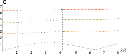
Figure 1: Excitation spectrum $\epsilon(\tilde{k})$ as a function of $\tilde{k}=kR$ for $\mu/\hbar\omega=5.9$ ($\beta=50$), $\eta=1.8$ ($R/l_{H}=3.45,\Delta=1.5nK,\omega=280Hz,\mu=68nK$). Two vertical dashed lines define a region where analytical form of the excitation spectrum does not exist.

Omitting the term $-\frac{(\eta-1)\tilde{k}^{2}s}{6\eta}W$ (which will be taken into account perturbatively later), equation (33) becomes a hypergeometric equation. The solution regular at the origin and finite for $s\to 1$ is

$$W_{j}=\tilde{C}F\left(-j,j+2,1,s\right),\,$$ (35)

where $j$ is a non-negative integer, and $\tilde{C}$ is the normalization constant. The related energy spectrum is given by $\epsilon_{j}^{2}=\epsilon_{*}^{2}(q)+\frac{3\eta}{1+\eta/2}j(j+2)$. From equations (21) and (22) in the limit of $kR\gg 1$ we have

$$f^{+}\approx\frac{4\mu\epsilon}{\hbar\omega\tilde{k}^{2}}f^{-},$$ (36)

and, hence,

$$f^{+}=\sqrt{\frac{4\mu\epsilon}{\hbar\omega\tilde{k}^{2}}}\frac{\sqrt{1-\tilde{\rho}^{2}}\,W}{\sqrt{\int d^{2}\tilde{\rho}\,(1-\tilde{\rho}^{2})W^{2}}}e^{ikz},$$ (37)

$$f^{-}=\sqrt{\frac{\hbar\omega\tilde{k}^{2}}{4\mu\epsilon}}\frac{\sqrt{1-\tilde{\rho}^{2}}\,W}{\sqrt{\int d^{2}\tilde{\rho}\,(1-\tilde{\rho}^{2})W^{2}}}e^{ikz}.$$ (38)

Adding the first order correction to $\epsilon_{j}^{2}$ from the omitted term $-\frac{(\eta-1)\tilde{k}^{2}s}{6\eta}W$, we obtain

$$\epsilon_{j}^{2}=\epsilon_{*}^{2}(\tilde{k})+\frac{1}{2}\frac{\eta-1}{1+\eta/2}\tilde{k}^{2}x_{j}+\frac{3\eta}{1+\eta/2}j(j+2),$$ (39)

where $x_{0}=1/3$, $x_{1}=7/15$, $x_{2}=17/35$, $x_{3}=31/63$,… Note that in the considered approximation the roton spectrum exists only at $\eta>1$. The typical spectrum is shown in Fig.1 for $\eta=1.8$. The lowest branch (in blue) has a roton.

The character of the spectrum is determined by two parameters: $\eta$ and $\mu/\hbar\omega$. Having in mind direct numerical calculations given below, instead of $\mu/\hbar\omega$ we will use the parameter $\beta=2nr_{*}$, where $r_{*}=md^{2}/\hbar^{2}$ is the so called dipolar length. For isotropic condensate wave function we have

$$\mu/\hbar\omega=\sqrt{(2+\eta)\beta/3\eta}.$$ (40)

IV Approximaton of isotropic condensate. Damping of rotons.

Substituting solutions (28), (29), (37), (38) into Eq.  (10). and integrating over the momentum $p$ and coordinates, we obtain for the damping rate of a roton with momentum $k$ the expression

$$\frac{1}{\tau_{jl}}=\frac{n_{0}g^{2}}{4\hbar R^{2}}\frac{N_{p,j}-N_{q+p,l}}{|E^{\prime}_{q+p,l}-E^{\prime}_{p,j}|}Z_{jl},$$ (41)

$$\begin{split}&Z_{jl}=\left[G_{1}(q)\bar{f}^{-}_{q,0}f^{+}_{p,j}\bar{f}^{+}_{q+p,l}+G_{2}(q)\bar{f}^{-}_{q,0}\bar{f}^{-}_{p,j}\bar{f}^{-}_{q+p,l}\right.\\ &+G_{3}(p)(\bar{f}^{-}_{p,j}\bar{f}^{+}_{q,0}\bar{f}^{+}_{q+p,l}+\bar{f}^{-}_{p,j}\bar{f}^{-}_{q,0}\bar{f}^{-}_{q+p,l})\\ &\left.-G_{1}(q+p)\bar{f}^{-}_{q+p,l}\bar{f}^{+}_{q,0}\bar{f}^{+}_{p,j}+G_{2}(q+p)\bar{f}^{-}_{q+p,l}\bar{f}^{-}_{p,j}\bar{f}^{-}_{q,0}\right]^{2},\\ \end{split}$$ (42)

where $E^{\prime}_{k,l}=dE_{k,l}/dk$, and the momentum $p$ is found from the energy conservation law:

$$E_{q+p,l}=E_{q,0}+E_{p,j}.$$ (43)

The functions $\bar{f}^{\pm}$ are coefficients in Eqs. (28), (29), (37), and (38):

$$\bar{f}^{\pm}_{p,j}=\left[\frac{2\mu}{\hbar\omega\epsilon_{p,j}}\right]^{\pm\frac{1}{2}},\quad\bar{f}^{\pm}_{q,l}=\left[\frac{4\mu\epsilon_{q,l}}{\hbar\omega\tilde{q}^{2}}\right]^{\pm\frac{1}{2}}.$$

For the functions $G_{i}$ we obtain by the use of Eqs. (23) - (24) the following expressions:

$$\begin{split}G_{1}(k)=\frac{(\epsilon_{k,l}^{2}-\left(\frac{\hbar\omega}{4\mu}\right)^{2}\tilde{k}^{4})(2+\eta)}{\tilde{k}^{2}}\\ \times\frac{\int_{0}^{1}(1-s)F_{1}F_{2}ds}{\sqrt{\int F_{1}^{2}ds}\sqrt{\int(1-s)F_{2}^{2}ds}},\end{split}$$ (44)

$$\begin{split}G_{2}(k)=\frac{(\epsilon_{k,l}^{2}-\left(\frac{\hbar\omega}{4\mu}\right)^{2}\tilde{k}^{4})(2+\eta)}{\tilde{k}^{2}}\\ \times\frac{\int_{0}^{1}F_{1}F_{2}ds}{\sqrt{\int(1-s)F_{1}^{2}ds}\sqrt{\int(1-s)F_{2}^{2}ds}},\end{split}$$ (45)

$$G_{3}(p)=(1+\eta/2)\frac{\int_{0}^{1}(1-s)F_{1}F_{2}ds}{\sqrt{\int F_{1}^{2}ds}\sqrt{\int(1-s)F_{2}^{2}ds}},$$ (46)

where $F_{1,2}$ are the hypergeometric functions: $F_{1}\equiv F(-j,j+1,1,s)$, $F_{2}\equiv F(-l,l+2,1,s)$, and we assume in Eqs. (43) - (45) that $pR\ll 1$, $kR\gg 1$. Hence, the quantity $Z_{jl}$ is a function of the parameters $\eta$ and $\mu/\hbar\omega$.

At temperatures greatly exceeding $\hbar\omega$ the occupation numbers are $N_{k}\approx T/E_{k}$, and, consequently, the damping rates are linear in $T$:

$$\frac{1}{\tau_{jl}}=\frac{k_{B}T}{\hbar}\frac{mg}{\hbar^{2}R}\alpha_{jl}Z_{jl},$$ (47)

where

$$\alpha_{jl}=\left[\frac{1}{\epsilon_{p,j}}-\frac{1}{\epsilon_{q+p,l}}\right]\frac{1}{|\epsilon^{\prime}_{q+p,l}-\epsilon^{\prime}_{p,j}|}$$ (48)

and this quantity is responsible for the increase of the damping rate in the limit of vanishingly small roton gap $\Delta\equiv\epsilon_{0}(q)$. For example, $\alpha_{00}\propto 1/\Delta$ at $\Delta\to 0$. For a very small gap the roton excitation is unstable due to strong decay processes. Its energy becomes of the order of $\hbar/\tau$ or even smaller.

We estimate now the damping rate for some values of dimensionless parameters $\beta$ and $\eta$ for dysprosium atoms ($r_{*}=200\AA$).

For $\mu/\hbar\omega=7.2$ ($\beta=70$), $\eta=1.6$, $\omega=340Hz$ we have $\Delta=0.9nK,\mu=101nK,R=1.6\cdot 10^{-4}cm$. The main decay channel in this case is the one with $j=0$, $l=0$. The damping rate reaches the value $\frac{1}{\tau}\sim 10s^{-1}$ at $T\sim 100nK$.

A decrease of ${\mu}/{\hbar\omega}$ may increase the number of decay channels. In particular, for ${\mu}/{\hbar\omega}=5.9$ ($\beta=50$), $\eta=1.8$, $\omega=280Hz$, we have $\Delta=1.5nK,\mu=68nK,R=1.6\cdot 10^{-4}cm$ and there are two channels: $j=0$, $l=0$; and $j=3$, $l=2$. The total damping rate at $T\sim 100nK$ becomes of the order of $\frac{1}{\tau}\sim 10^{2}s^{-1}$.

For all data the damping rate is much smaller than the roton energy: $\hbar/(\Delta\tau)\ll 1$. Therefore, the roton is a well defined excitation.

V Direct numerical calculations

V.1 Condensate wave function and excitation spectrum

In this section we present our numerical results for the ground state wave function and excitation spectrum of the condensate. We numerically solved the GPE equation (1) for $\Psi_{0}(x,y)$ using the imaginary-time evolution algorithm in 2D Cartesian grid. The Bogoliubov-de Gennes equations (4) - (5) for the excitation spectrum are solved using the large-scale Krylov-Schur eigensolver.

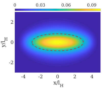
Figure 2: The density of the condensate plotted in the $x,y$ plane for $\beta=50$ and $\eta=1.231$. The dashed red line is the countour plot at half-width of the condesate density. The condensate form is anistropic with elongation in the direction of dipoles.

In Figs. 2 and 3 we present the condensate density distribution and the excitation spectrum in the transverse direction for the dimensionless parameters $\beta=50$ and $\eta=1.231$. In Fig. 2 the length scale is in units of harmonic oscillator length $l_{H}$. Our numerical results for the condensate wavefunction show its anisotropic form with elongation in the direction of dipoles, as shown in Fig. 2. The red dashed curve in the figure marks the countour plot at half-width of the condesate density.

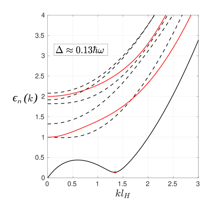
Figure 3: Low-lying excitation branches $\epsilon_{n}(k)$ as a function of $kl_{H}$ for $\beta=50$ and $\eta=1.231$. The branches are labelled with an index $n$ based on their value at $k=0$ starting from $n=0$. Only the lowest branch $\epsilon_{0}(k)$ has a roton-type excitation with the rotonic gap $\Delta\approx 0.13\hbar\omega$. The largest contribution to the roton damping comes from the intraband transitions in the the excitation branches $\epsilon_{2}(k)$ and $\epsilon_{6}(k)$ (red solid curves).

The excitation spectrum $E_{k}$ consists of an infinite number of branches. We considered only eight low-lying branches, which is enough for our purposes. As clear from Fig. 3, only the lowest band contains a roton type excitation with the rotonic gap $\Delta\approx 0.13\hbar\omega$ at $kl_{H}\approx 1.33$ for the dimensionless parameters given above. At a fixed parameter $\beta=50$, increasing/decreasing $\eta$ modifies the excitation spectrum and decreases/increases the rotonic gap $\Delta$. For $\eta\lesssim 1.2$ the rotonic minimum disappears, and there are no rotonic excitations. On the other hand, for $\eta_{c}\approx 1.2325$ the rotonic gap goes to zero, and for larger $\eta$ the condensate uniform in the $z$ direction is unstable. For comparison, for a larger value $\beta=104$ the rotonic excitation appears at $\eta\approx 1.12$ and the rotonic gap vanishes at $\eta_{c}\approx 1.147$.

V.2 Damping rate for rotons

Using the solutions of the Bogoliubov-de Gennes equations we calculate the damping rate for the roton excitations with the help of expression (10). Due to the broken rotational symmetry, the projection of angular momentum on the $z$-axis is not a conserved quantity and does not serve as a good quantum number. Thus, both intraband ($n_{1}=n_{2}$ in Eq. (10)) and interband ($n_{1}\neq n_{2}$ in Eq. (10)) transitions can contribute to the damping rate of the rotonic excitation.

We first present the rates for $\beta=50$ and $\eta=1.231$ and fix the trap frequency $\omega=280Hz$. Our numerical results show that the main contribution to the damping rate is given by the intraband transition within the third band, i.e the transition with $n_{1}=n_{2}=2$ with $1/\tau_{2,2}=75s^{-1}$ at $T=100nK$. To compare, the damping rate due to the transition in the rotonic branch is $1/\tau_{0,0}=23.9s^{-1}$. Such large contribution of $1/\tau_{2,2}$ results from relatively large matrix elements $A^{q}_{k,k+q}$ and large density of states (vanishingly small velocity difference in Eq. (41)). The contributions of intraband transitions in higher bands are suppressed due to small matrix elements. As an example, the next largest contribution to the damping rate from the intraband transition is $1/\tau_{6,6}=4.8s^{-1}\ll 1/\tau_{2,2}$. The total damping rate from all other intraband transitions is smaller than $1/\tau_{6,6}$.

Similarly, our result for the total damping rate due to all possible interband transitions is smaller than $5s^{-1}$. Although such transitions are not prohibited, practically typical matrix elements are smaller by orders of magnitude. We also considered the damping rates in three other regimes, achieved by varying $\eta$ at $\beta=50$. We estimated the damping rates at $\eta=\{1.225,1.231,1.232,1.2323\}$ and presented our final results in Table I. The total damping rate at $T=100nK$ increases with decreasing the rotonic gap from $1/\tau=20.4s^{-1}$ at $\Delta=0.28\hbar\omega$ up to $1/\tau=214.5s^{-1}$ at $\Delta=0.06\hbar\omega$. Finally, we plot the temperature dependance of the damping rates in Fig. 4.

Table 1: Damping rates $\tau_{n,n}^{-1}$ in units of $s^{-1}$ given at $T=100nK$ at different system parameters $\eta$ with the rotonic gaps $\Delta$. The values $\beta=50$ and $\omega=280Hz$ are kept fixed.

$\eta$	$\Delta/{\hbar\omega}$	$\tau_{0,0}^{-1}$	$\tau_{2,2}^{-1}$	$\tau_{6,6}^{-1}$	$\tau^{-1}$
$1.225$	$0.28$	$4.9$	$15.2$	$0.3$	$20.4$
$1.231$	$0.13$	$23.9$	$75$	$2.4$	$101.3$
$1.232$	$0.09$	$29.4$	$129.6$	$4.8$	$163.8$
$1.2323$	$0.06$	$30.6$	$178.2$	$5.7$	$214.5$

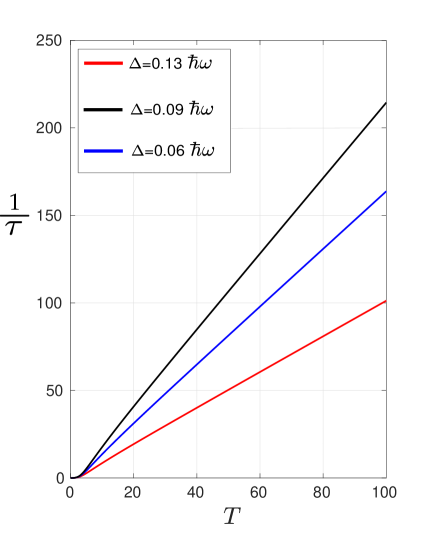
Figure 4: The total damping rates $1/\tau$ in units of $s^{-1}$ versus temperature $T$ given in $nK$ for $\omega=280Hz$ and $\beta=50$ in three different regimes with [ $\eta=1.231$, $\Delta=0.13\hbar\omega$ (red) ], [ $\eta=1.232$, $\Delta=0.09\hbar\omega$ (blue) ] and [ $\eta=1.2323$, $\Delta=0.06\hbar\omega$ (black) ].

VI Conclusions

In this paper we have calculated the finite temperature damping rate for rotons in an elongated Bose-condensed gas of polarized dipolar particles, which is in the Thomas-Fermi regime in the tightly confined directions. The important feature of this case is the presence of a large number of excitation branches which can contribute to the damping process. We found out that this leads to a significant increase of the damping rate. Nevertheless, our calculations show that, even in this regime, rotons in systems with the roton energy gap of the order of $1\,nK$ are sufficiently long-living and can be observed as well-defined peaks in the excitation spectrum and contributions in response functions.

- [1] E. P. Gross, Classical theory of boson wave fields, Ann. Phys. (N.Y.)4, 57 (1958).
- [2] P. Nozi‘eres, J. Low Temp. Phys. 137, 45 (2004).
- [3] D. H. J. O’Dell, S. Giovanazzi, and G. Kurizki, Phys. Rev. Lett. 90, 110402 (2003).
- [4] L. Santos, G. V. Shlyapnikov, and M. Lewenstein, Phys. Rev. Lett. 90, 250403 (2003).
- [5] M. Boninsegni and N. V. Prokof’ev, Rev. Mod. Phys. 84, 759 (2012).
- [6] F. Böttcher, J.-N. Schmidt, M.Wenzel, J. Hertkorn, M. Guo, T. Langen, and T. Pfau, Phys. Rev. X 9, 011051 (2019).
- [7] L. Tanzi, E. Lucioni, F. Fam‘a, J. Catani, A. Fioretti, C. Gabbanini, R. N. Bisset, L. Santos, and G. Modugno, Phys. Rev. Lett. 122, 130405 (2019).
- [8] L. Chomaz, D. Petter, P. Ilzhöfer, G. Natale, A. Trautmann, C. Politi, G. Durastante, R. M. W. van Bijnen, A. Patscheider, M. Sohmen, M. J. Mark, and F. Ferlaino, Phys. Rev. X 9, 021012 (2019).
- [9] L. Chomaz, R. M.W. van Bijnen, D. Petter, G. Faraoni, S. Baier, J. H. Becher, M. J. Mark, F. Wächtler, L. Santos, and F. Ferlaino, Nat. Phys. 14, 442 (2018).
- [10] D. Petter, G. Natale, R. M.W. van Bijnen, A. Patscheider, M. J. Mark, L. Chomaz, and F. Ferlaino, Phys. Rev. Lett. 122, 183401 (2019)
- [11] J.-N. Schmidt , J. Hertkorn , M. Guo, F. Böttcher , M. Schmidt, K. S. H. Ng, S. D. Graham, T. Langen, M. Zwierlein, and T. Pfau, Roton Excitations in an Oblate Dipolar Quantum Gas, Phys. Rev. Lett. 126, 193002, (2021).
- [12] G. Natale, R. van Bijnen, A. Patscheider, D. Petter, M. J. Mark, L. Chomaz, F. Ferlaino, Phys. Rev. Lett. 123, 50402 (2019).
- [13] J. Hertkorn, F. Böttcher, M. Guo, J. N. Schmidt, T. Langen, H. P. Büchler, and T. Pfau, Phys. Rev. Lett. 123, 193002 (2019).
- [14] D. Petter, A. Patscheider, G. Natale, M. J. Mark , M. A. Baranov, R. van Bijnen, S. M. Roccuzzo, A. Recati, B. Blakie, D. Baillie, L. Chomaz, and F. Ferlaino, Phys. Rev. A 104, L011302 (2021).
- [15] S. S. Natu, L. Companello, and S. Das Sarma, Phys. Rev. A 90, 043617 (2014).
- [16] M. Jona-Lasinio, K. Lakomy, and L. Santos, Phys. Rev. A 88, 013619 (2013).
- [17] H. Kurkjian, Z. Ristivojevic, Phys. Rev. Research 2, 033337 (2020).
- [18] S. S. Natu, R. M. Wilson, Phys. Rev. A 88 063638 (2013); R. M. Wilson S. S. Natu, Phys. Rev. A 93, 053606 (2016).
- [19] J. T. Mendonça, H. Terças, A. Gammal, Phys. Rev. A 97, 063610 (2018).
- [20] D.H.J. O’Dell, S. Giovanazzi, and C. Eberlein, Phys. Rev. Lett. 92, 250401 (2004).
- [21] C. Eberlein, S. Giovanazzi, and D.H.J. O’Dell, Phys. Rev. A 71, 033618 (2005).
- [22] L. Pitaevskii and S. Stringari, Bose-Einstein Condensation and Superfluidity (Oxford University Press, Oxford, 2016), Vol. 164.