Power-law holographic dark energy and cosmology

Abstract

We formulate power-law holographic dark energy, which is a modified holographic dark energy model based on the extended entropy relation arising from the consideration of state mixing between the ground and the excited ones in the calculation of the entanglement entropy. We construct two cases of the scenario, imposing the usual future event horizon choice, as well as the Hubble one. Thus, the former model is a one-parameter extension of standard holographic dark energy, recovering it in the limit where power-law extended entropy recovers Bekenstein-Hawking one, while the latter belongs to the class of running vacuum models, a feature that may reveal the connection between holography and the renormalization group running. For both models we extract the differential equation that determines the evolution of the dark-energy density parameter and we provide the expression for the corresponding equation-of-state parameter. We find that the scenario can describe the sequence of epochs in the Universe evolution, namely the domination of matter followed by the domination of dark energy. Moreover, the dark-energy equation of state presents a rich behavior, lying in the quintessence regime or passing into the phantom one too, depending on the values of the two model parameters, a behavior that is richer than the one of standard holographic dark energy.

I Introduction

According to accumulating observational evidence, the Universe has exhibited the transition to the accelerated era in the recent cosmological past. One can attribute this unexpected feature in the presence of the cosmological constant, however the corresponding problem related to the smallness of its observed value, as well as the possibility that the acceleration has a dynamical nature, has led to a variety of other possibilities. A first avenue of modification of the standard cosmological paradigm is to introduce the concept of dark energy Copeland:2006wr ; Cai:2009zp ; Bamba:2012cp . The second road that one can follow is to modify the gravitational theory itself, resulting to theories that exhibit richer structure and phenomenology that could eventually lead to an accelerating Universe Nojiri:2010wj ; Capozziello:2011et ; Cai:2015emx ; CANTATA:2021ktz .

Holographic dark energy is a different alternative that can provide the explanation for the Universe acceleration. The basis of this scenario is the holographic principle tHooft:1993dmi ; Susskind:1994vu ; Bousso:2002ju , applied in a cosmological framework Fischler:1998st ; Bak:1999hd ; Horava:2000tb . In particular, since the largest distance of a quantum field theory, required for its applicability at large distances, is related to its ultra-violet (UV) cutoff, which is in turn related to the vacuum energy Cohen:1998zx ; Addazi:2021xuf , one can attribute a holographic origin to the vacuum energy, which will then be a form of holographic dark energy Li:2004rb ; Wang:2016och . Holographic dark energy has been shown to exhibit very interesting cosmological phenomenology Li:2004rb ; Wang:2016och ; Horvat:2004vn ; Huang:2004ai ; Pavon:2005yx ; Wang:2005jx ; Nojiri:2005pu ; Kim:2005at ; Setare:2006wh ; Setare:2008hm ; Sheykhi:2009dz ; Li:2009bn ; Zhang:2009un ; Micheletti:2010cm ; Lu:2009iv ; Micheletti:2009jy ; Aviles:2011sfa ; Luongo:2017yta , and additionally a large amount of research has been devoted to its extensions.

There are two main ways of extending the basic scenario of holographic dark energy. The first is to apply different horizons for the Universe, such as the event horizon, the apparent horizon, the age of the universe, the conformal time, the inverse square root of the Ricci curvature and the Gauss Bonnet term, etc Gong:2004fq ; Saridakis:2007cy ; Cai:2007us ; Setare:2008bb ; Gong:2009dc ; Suwa:2009gm ; Jamil:2010vr ; BouhmadiLopez:2011xi ; Malekjani:2012bw ; Khurshudyan:2014axa ; Landim:2015hqa ; Shekh:2021ule . On the other hand, the second possibility of modification is the consideration of a modified entropy expression for the Universe horizon instead of the standard Bekenstein-Hawking one, such as Tsallis entropy, Barrow entropy, Kaniadakis entropy, logarithmic corrected entropy etc Pasqua:2015bfz ; Jawad:2016tne ; Pourhassan:2017cba ; Saridakis:2017rdo ; Nojiri:2017opc ; Saridakis:2018unr ; DAgostino:2019wko ; Saridakis:2020zol ; Dabrowski:2020atl ; daSilva:2020bdc ; Anagnostopoulos:2020ctz ; Mamon:2020spa ; Bhattacharjee:2020ixg ; Huang:2021zgj ; Drepanou:2021jiv ; Hossienkhani:2021emv ; Nojiri:2021iko ; Jusufi:2021fek ; Hernandez-Almada:2021aiw ; Hernandez-Almada:2021rjs ; Luciano:2022pzg .

Attributing an entropy to a horizon, and in particular relating it to its area, is connected with the topological restrictions of quantum interactions of quantum states and emerges from seemingly distinct areas in physics, such as black holes, quantum field theory, information theory, and quantum many-body physics Eisert:2008ur . The first to suggest an area-law dependence of the black hole entropy was Bekenstein Bekenstein:1973ur , who, based on information theory and dimensional arguments, derived the well known formula, that was later specified by Hawking Hawking:1975vcx , namely the Bekenstein-Hawking entropy $S_{BH}=\frac{A}{4l_{P}^{2}}$, where $A$ is the horizon area and $l_{P}$ the Planck length, in units $k_{{}_{B}}=c=\hbar=1$. This kind of behaviour was verified as compatible with the notion of quantum gravity through the holographic principle. An identical entropy behaviour reproducing the area law, was also derived by Bombelli Bombelli:1986rw and later by Srednicki Srednicki:1993im , for the entanglement entropy of a spherical region in the case of scalar massless fields, and this concurrence is not thought to be accidental. Indeed, from the recent developments in AdS/CFT correspondence Maldacena:1997re and the Ryu-Takayanagi formula Ryu:2006bv , to the concept of emergent gravity Sakharov:1967pk , indications appear to agree on a deeper connection among the manifestations of the area law.

In the calculation of the entanglement entropy one starts from the vacuum ground state. However, adding the excited states one obtains a power-law correction in the entanglement entropy. In particular, considering a 1-particle excitation one results to a modified entropy relation of the form Das:2007mj ; Radicella:2010ss

$$S=S_{BH}+c\left(\frac{A}{\epsilon^{2}}\right)^{-\gamma},$$ (1)

where the exponent $\gamma$ depends on the degree of mixing of the ground state with the excited one, varying between -1 and 0, and $c$ is a constant. Furthermore, $\epsilon$ is the UV cutoff of the scalar field theory used to derive the entropy, and in the following we will set it equal to the Plank length $l_{p}=M_{p}^{-1}$, where $M_{p}$ the Plank mass. Hence, the above expression for $c=0$ recovers the standard Bekenstein-Hawking entropy, while for $\gamma=0$ we obtain the topological entropy constant term Kitaev:2005dm .

In this work we will apply the power-law entropy relation in order to formulate holographic dark energy, and study its cosmological implications. Although in the literature there were some attempts towards this direction, they remained incomplete with complete absence of cosmological applications Sheykhi:2011egx ; Khodam-Mohammadi:2011oji ; Ebrahimi:2010xz ; Pasqua:2012hm . The plan of the manuscript is the following: In Section II we formulate power-law holographic dark energy, presenting the corresponding cosmological equations and extracting the expressions for the dark energy density and equation-of-state parameters, focusing on two cases of the horizon choice. In Section III we investigate the resulting cosmological behavior. Lastly, in Section IV we summarize the obtained results.

II Power-law holographic dark energy

In this section we formulate power-law holographic dark energy. We start be recalling that holographic dark energy arises from the inequality $\rho_{DE}L^{4}\leq S$, with $L$ the Universe horizon and $S$ the black-hole entropy relation applied for $L$ Li:2004rb ; Wang:2016och . If we use the standard Bekenstein-Hawking entropy $S_{BH}\propto AM_{p}^{2}/4=\pi M_{p}^{2}L^{2}$, then the saturation of the previous inequality provides standard holographic dark energy, i.e. $\rho_{DE}=3c_{1}^{2}M_{p}^{2}L^{-2}$, with $c_{1}$ the model parameter.

However, as we mentioned in the Introduction, there are many modifications of Bekenstein-Hawking entropy. One of them is the power-law extended entropy (1), which arises from the consideration of the mixing of excited states with the ground one in the entanglement entropy Das:2007mj . Re-expressing it as $S=S_{BH}+cS_{BH}^{-\gamma}$ and inserting it in the inequality $\rho_{DE}L^{4}\leq S$ we acquire

$$\rho_{DE}=c_{1}\pi M_{p}^{2}L^{-2}+c_{2}\left(\pi M_{p}^{2}\right)^{-\gamma}L^{-2\gamma-4},$$ (2)

where $c_{1}$ and $c_{2}$ are dimensionless constants (the parameter $c$ has been absorbed in $c_{2}$) and thus in units $k_{{}_{B}}=c=\hbar=1$ the energy density has units of $[M]^{4}$ as expected. Therefore, as mentioned above, for $c_{2}=0$ the above expression becomes the standard holographic dark energy $\rho_{DE}=3c_{1}^{2}M_{p}^{2}L^{-2}$.

As usual, we consider a flat Friedmann-Robertson-Walker (FRW) metric of the form

$$ds^{2}=-dt^{2}+a^{2}(t)\delta_{ij}dx^{i}dx^{j}\,,$$ (3)

with $a(t)$ the scale factor. Given this geometry we have two choices for the maximum length $L$ that appears in the above relations. In the case of usual holographic dark energy one can show that $L$ cannot be the Hubble horizon $H^{-1}$ (with $H\equiv\dot{a}/a$ the Hubble function), since the resulting model cannot lead to acceleration Hsu:2004ri . Therefore, the standard choice is the future event horizon, defined as Li:2004rb

$$R_{h}\equiv a\int_{t}^{\infty}\frac{dt}{a}=a\int_{a}^{\infty}\frac{da}{Ha^{2}}.$$ (4)

Hence, in the following we will use $R_{h}$ as the IR cutoff of the theory. However, since the present scenario is a novel one, we do have the choice to use the Hubble horizon $H^{-1}$ as $L$, since the resulting model can indeed describe acceleration. In the following subsections we will study these two cases separately.

II.1 Model 1: Holography on the future event horizon

Let us use the future event horizon $R_{h}$ of (4) as the infra-red (IR) cutoff. In this case, the holographic dark energy density (2) will be

$$\rho_{DE}=c_{1}\pi M_{p}^{2}R_{h}^{-2}+c_{2}\left(\pi M_{p}^{2}\right)^{-\gamma}R_{h}^{-2\gamma-4}.$$ (5)

Moreover, the two Friedmann equations in a universe containing the aforementioned holographic dark energy, as well as the matter perfect fluid, are written as

$$3M_{p}^{2}H^{2} = \ \rho_{m}+\rho_{DE}$$ (6)

$$-2M_{p}^{2}\dot{H} = \rho_{m}+p_{m}+\rho_{DE}+p_{DE},$$ (7)

with $p_{DE}$ the pressure of the power-law holographic dark energy, and $\rho_{m}$, $p_{m}$ the matter energy density and pressure respectively. Note that we can additionally consider the matter conservation equation

$$\dot{\rho}_{m}+3H(\rho_{m}+p_{m})=0,$$ (8)

which according to Friedmann equations then implies the dark-energy conservation equation

$$\dot{\rho}_{DE}+3H(\rho_{DE}+p_{DE})=0.$$ (9)

We proceed by introducing the density parameters of the dark energy and matter sector as

$$\Omega_{m}\equiv\frac{1}{3M_{p}^{2}H^{2}}\rho_{m}$$ (10)

$$\Omega_{DE}\equiv\frac{1}{3M_{p}^{2}H^{2}}\rho_{DE}.$$ (11)

Furthermore, inserting (11) into (5) gives

$$\Omega_{DE}H^{2}=C_{1}R_{h}^{-2}+C_{2}R_{h}^{-2\gamma-4},$$ (12)

with $C_{1}\equiv\frac{c_{1}\pi}{3}$ and $C_{2}\equiv\frac{c_{2}\pi^{-\gamma}M_{p}^{-2+2\gamma}}{3}$ the model parameters. On the other hand, differentiating (4) with respect to time we obtain the useful relation $\dot{R}_{h}=HR_{h}-1$, and if we use $x=\ln a$ as the independent variable it gives rise to

$$R_{h}^{\prime}=R_{h}-H^{-1},$$ (13)

with primes denoting derivatives with respect to $x$. Hence, taking the $x$-derivative of (12) and using (13), we finally obtain

$$\tilde{\Omega}(F^{\prime}+\tilde{F}^{\prime}+2^{\frac{1}{3}}Q^{\prime})-\tilde{\Omega}^{\prime}(F+\tilde{F}+2^{\frac{1}{3}}Q)$$

$$-\tilde{\Omega}(F+\tilde{F}+2^{\frac{1}{3}}Q)+3H^{-1}2^{\frac{1}{3}}\tilde{\Omega}^{2}=0,$$ (14)

where

$$Q=(2\gamma+4)\Omega_{DE}H,$$

$$\tilde{\Omega}=(\Omega_{DE}H^{2})^{\prime}+HQ,$$

$$A=18C_{1}(\gamma+1)\tilde{\Omega}(1+3H^{-1}\tilde{\Omega})+2Q^{3},$$

$$B=-6C_{1}(\gamma+1)\tilde{\Omega}-Q^{2},$$

$$F=(\sqrt{A^{2}+4B^{3}}+A)^{\frac{1}{3}},$$

$$\tilde{F}=(-\sqrt{A^{2}+4B^{3}}+A)^{\frac{1}{3}}.$$ (15)

Note that the derivatives of $H$ in the above formulas can be expressed in terms of derivatives of $\Omega_{DE}$ through the simple relation

$$\frac{1}{Ha}=\frac{\sqrt{a(1-\Omega_{DE})}}{H_{0}\sqrt{\Omega_{m0}}},$$ (16)

which is just the first Friedmann equation (6) in the case of dust matter, i.e $p_{m}=0$, in which case (8) leads to $\Omega_{m}=\Omega_{m0}/a^{3}$, with the subscript “0” denoting the present values of a quantity.

In summary, equation (14) is a second-order differential equation for $\Omega_{DE}$ as a function of $x=\ln a$, and hence it determines the evolution of power-law holographic dark energy. As expected, in the case $C_{2}=0$ it recovers the corresponding differential equation of standard holographic dark energy Li:2004rb , namely $\Omega_{DE}^{\prime}=\Omega_{DE}(1-\Omega_{DE})\left(1+2\sqrt{\frac{3M_{p}^{2}\Omega_{DE}}{3c_{1}^{2}M_{p}^{2}}}\right)$, which is solved in an implicit form Li:2004rb .

Concerning the important observable $w_{DE}\equiv p_{DE}/\rho_{DE}$, namely the dark-energy equation-of-state parameter, from the conservation equation (9) we obtain $\rho_{DE}^{\prime}+3\rho_{DE}(1+w_{DE})=0$, which using the density parameter and the definitions (15) gives

$$w_{DE}=-1+\frac{HQ-\tilde{\Omega}}{3H^{2}\Omega_{DE}}.$$ (17)

Thus, knowing $\Omega_{DE}$ from (14) allows us to calculate $w_{DE}$ as a function of $\ln a$. Once again we mention that for $C_{2}=0$ expression (17) provides the result of standard holographic dark energy, that is $w_{DE}=-\frac{1}{3}-\frac{2}{3}\frac{\sqrt{\Omega_{DE}}}{c}$ Wang:2016och , as expected. Note that $w_{DE}$ can be quintessence-like or phantom-like according to the model parameter choices. Lastly, it proves convenient to introduce the deceleration parameter

$$q\equiv-1-\frac{\dot{H}}{H^{2}}=\frac{1}{2}+\frac{3}{2}\left(w_{m}\Omega_{m}+w_{DE}\Omega_{DE}\right),$$ (18)

which for dust matter ($w_{m}=0$) can be straightforwardly found if $\Omega_{DE}$ (and therefore $w_{DE}$) is known.

II.2 Model 2: Holography on the Hubble horizon

We proceed to the construction of a different scenario, which arises from the use of the Hubble horizon $H^{-1}$ as the IR cutoff. In this case, the holographic dark energy density (2) will be simply

$$\rho_{DE}=\tilde{c}_{1}H^{2}+\tilde{c}_{2}H^{2\gamma+4},$$ (19)

with $\tilde{c}_{1}=c_{1}\pi M_{p}^{2}$ and $\tilde{c}_{2}=c_{2}\left(\pi M_{p}^{2}\right)^{-\gamma}$. We stress here that this scenario does not possess standard holographic dark energy as a particular limit in the case where the power-law entropy becomes standard Bekenstein-Hawking one (i.e. for $c_{2}=0$) however it can be a very efficient cosmological scenario, being able to describe acceleration. The reason is that when the second term in the rhs of (19) is present the dark energy density obtains richer behavior, which is impossible in the case of its absence. Actually it was due to this feature that in the initial formulation of holographic dark energy the event horizon was used instead of the Hubble one Li:2004rb , however in the present power-law extension this complication is not needed, since the Hubble horizon can perfectly be used as the IR cutoff.

Interestingly enough, the energy density (19) belongs to the class of running vacuum models Shapiro:2009dh ; Perico:2013mna , which may reveal the connection between holography and the renormalization group running Shapiro:2000dz ; Basilakos:2019acj . Inserting (19) into the Friedmann equation (6) and using (16) we obtain

$$\Omega_{DE}=\tilde{C}_{1}+\tilde{C}_{2}\left[\frac{H_{0}^{2}\Omega_{m0}}{a^{3}\left(1-\Omega_{DE}\right)}\right]^{\gamma+1},$$ (20)

with $\tilde{C}_{1}\equiv\tilde{c_{1}}/(3M_{p}^{2})$ and $\tilde{C}_{2}\equiv\tilde{c_{2}}/(3M_{p}^{2})$. Equation (20) is an algebraic equation for $\Omega_{DE}(a)$ which can then lead to $\Omega_{DE}(x)$ using $x=\ln a$. Additionally, the dark-energy equation-of-state parameter can straightforwardly arise by inserting (19) into the conservation equation $\rho_{DE}^{\prime}+3\rho_{DE}(1+w_{DE})=0$, and eliminating $H$ through (16), resulting to

$$w_{DE}=-\frac{\Omega_{DE}^{\prime}}{3\Omega_{DE}(1-\Omega_{DE})}.$$ (21)

Finally, the corresponding deceleration parameter results inserting the above expression into (18).

III Cosmological evolution

In the previous section we constructed power-law holographic dark energy in a consistent way, providing the differential equation that determines the evolution of the dark-energy density parameter and then the expression for the dark-energy equation of state. In this section we perform a detailed analysis of the cosmological evolution. We mention that we will focus mainly on Model 1, namely of the usual case of the event horizon, since the phenomenology of Model 2 belongs to that of running vacuum scenarios.

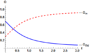
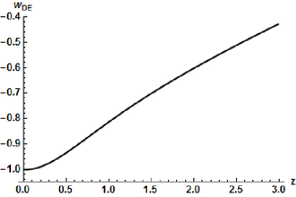
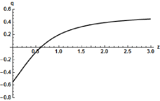
Figure 1: Upper graph: The power-law holographic dark energy density parameter $\Omega_{DE}$ (blue-solid) and the matter density parameter $\Omega_{m}$ (red-dashed), as a function of the redshift $z$, for Model 1, for $\gamma=0.4$ and $C_{1}=0.4$ in units where $k_{{}_{B}}=c=\hbar=M_{p}=1$. Middle graph: The corresponding dark-energy equation-of-state parameter $w_{DE}$. Lower graph: The corresponding deceleration parameter $q$. In all graphs we have imposed $\Omega_{DE}(x=-\ln(1+z)=0)\equiv\Omega_{DE0}\approx 0.7$.

In the case of Model 1, namely in the case where the IR cutoff is the future event horizon, since (14) can be solved analytically only when $C_{2}=0$, for the general case we solve it numerically. Additionally, in order to be closer to observations, we will use the redshift $z$ as the independent variable, which is related to the aforementioned variable $x$ through the simple relation $x\equiv\ln a=-\ln(1+z)$. Finally, as usual we impose $\Omega_{DE}(x=-\ln(1+z)=0)\equiv\Omega_{DE0}\approx 0.7$ Planck:2018vyg .

In Fig. 1 we present the evolution of the dark energy and matter density parameters (upper graph), of the dark-energy equation-of-state parameter $w_{DE}$ (middle graph), and of the deceleration parameter $q$ (lower graph). As we see, we can obtain the sequence of matter and dark energy eras as required by observations, and moreover the $w_{DE}$ at present is around $-1$, while being always in the quintessence regime. Furthermore, $q$ exhibits the transition from deceleration to acceleration at $z\approx 0.55$, in agreement with the value obtained by $\Lambda$CDM scenario Planck:2018vyg .

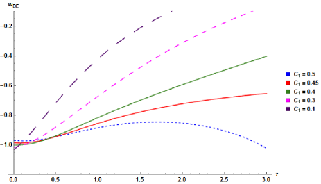
Figure 2: The redshift-evolution of the equation-of-state parameter $w_{DE}$ of power-law holographic dark energy of Model 1, for fixed $\gamma=0.5$ and various values of $C_{1}$ in units where $k_{{}_{B}}=c=\hbar=M_{p}=1$. We have imposed $\Omega_{DE0}\approx 0.7$.

Figure 3: The redshift-evolution of the equation-of-state parameter $w_{DE}$ of power-law holographic dark energy of Model 1, for fixed $C_{1}=0.35$ and various values of $\gamma$ in units where $k_{{}_{B}}=c=\hbar=M_{p}=1$. We have imposed $\Omega_{DE0}\approx 0.7$.

In order to investigate the effects of the model parameters $C_{1}$ and $\gamma$ on the cosmological evolution, we focus on the corresponding behavior of the dark-energy equation-of-state parameter $w_{DE}$. In Fig. 2 we show $w_{DE}(z)$ for fixed $\gamma$ and various values of $C_{1}$, where for all curves the corresponding evolution of the density parameters is similar to that of Fig. 1. As we observe, with increasing $C_{1}$ the values of $w_{DE}(z)$ at larger $z$ decrease, obtaining phantom values for $C_{1}>0.5$. On the other hand, the present-day value $w_{DE}(z=0)$ remains very close to -1 as required, however note that it can lie either in the quintessence regime or in the phantom one. Hence, according to the $C_{1}$ value, the dark-energy equation-of-state parameter can be quintessence-like, phantom-like, or experience the phantom-divide crossing during the evolution. Similarly, in Fig. 3 we depict the evolution of $w_{DE}(z)$ for fixed $C_{1}$ and various values of $\gamma$. In this case we see that for increasing $\gamma$, $w_{DE}$ acquires algebraically larger values at larger redshifts, while the present value $w_{DE}(z=0)$ is around -1, and can be either quintessence or phantom.

IV Conclusions

In the present work we formulated a holographic dark energy by considering the power-law extended entropy. This entropy relation arises from the consideration of state mixing between the ground and the excited ones in the calculation of the entanglement entropy Das:2007mj . The resulting power-law holographic dark energy can be applied in two horizon choices. In the first model we made the standard choice of the future event horizon as the IR cutoff, acquiring a one-parameter extension of standard holographic dark energy, recovering it in the limit where power-law extended entropy recovers Bekenstein-Hawking one. In the second model we used the Hubble horizon as the Universe horizon, and although this scenario does not possess standard holographic dark energy as a particular limit, it is a reasonable choice since in this case one does not face the usual problems which arise when trying to formulate standard holographic dark energy with the Hubble horizon.

We proceeded by extracting the differential equation that determines the evolution of the dark-energy density parameter of power-law holographic dark energy, and we provided the expression for the corresponding equation-of-state parameter, for both models. Thus, elaborating the equations we are able to investigate the resulting cosmological behavior.

Power-law holographic dark energy can describe the sequence of epochs in the Universe evolution, namely the domination of matter followed by the domination of dark energy, with the onset of acceleration taking place at $z\approx 0.55$. Furthermore, the dark-energy equation of state presents a rich behavior, lying in the quintessence regime or passing into the phantom one too, depending on the values of the two model parameters. As we saw, for fixed exponent $\gamma$ with increasing $C_{1}$ the values of $w_{DE}$ at larger $z$ decrease, obtaining phantom values for $C_{1}>0.5$. On the other hand, for fixed $C_{1}$ increasing $\gamma$ led to algebraically larger values at larger redshifts. This behavior is richer than the one of standard holographic dark energy, which was expected since the present model has one additional parameter.

Before closing this manuscript, let us make a comment on the confrontation with observational data. As it is known, the basic holographic dark energy model is less efficient in fitting the data comparing to $\Lambda$CDM cosmology Zhang:2005hs ; Huang:2004wt ; Wang:2005ph ; Feng:2007wn . On the other hand it is free from the fine-tuning problem of the latter, and moreover it has been shown to be able to alleviate the $H_{0}$ tension Abdalla:2022yfr . Thus, the field is open, and the community still devotes research on various extensions of holographic dark energy in order to examine whether they could be a viable candidate for the description of nature.

Hence, it would be interesting to proceed with a detailed confrontation with observations, in order to examine the cosmological capability of the scenario of power-law holographic dark energy, and more importantly to apply the known information criteria in order to compare its statistical efficiency with other scenarios, such as standard holographic dark energy and $\Lambda$CDM cosmology. In the same lines, we should study in detail the potential ability of the scenario to alleviate the $H_{0}$ and growth tensions. Finally, a necessary step is to perform a detailed investigation of the phase-space behavior, through a dynamical-system analysis that could reveal the global features of the universe evolution in such a scenario. These investigations lie beyond the present work and will be performed in following studies.

- (1) E. J. Copeland, M. Sami and S. Tsujikawa, Int. J. Mod. Phys. D15, 1753 (2006) [hep-th/0603057].
- (2) Y. -F. Cai, E. N. Saridakis, M. R. Setare and J. -Q. Xia, Phys. Rept. 493, 1 (2010) [0909.2776].
- (3) K. Bamba, S. Capozziello, S. Nojiri and S. D. Odintsov, Astrophys. Space Sci. 342, 155 (2012) [1205.3421].
- (4) S. Nojiri and S. D. Odintsov, Phys. Rept. 505, 59 (2011) [1011.0544 [gr-qc]].
- (5) S. Capozziello and M. De Laurentis, Phys. Rept. 509, 167 (2011) [1108.6266 [gr-qc]].
- (6) Y. F. Cai, S. Capozziello, M. De Laurentis and E. N. Saridakis, Rept. Prog. Phys. 79, 106901 (2016) [1511.07586].
- (7) E. N. Saridakis et al. [CANTATA], [2105.12582].
- (8) G. ’t Hooft, Salamfest 1993: 0284-296 [gr-qc/9310026].
- (9) L. Susskind, J. Math. Phys. 36, 6377 (1995) [hep-th/9409089].
- (10) R. Bousso, Rev. Mod. Phys. 74, 825 (2002) [hep-th/0203101].
- (11) W. Fischler and L. Susskind, [hep-th/9806039].
- (12) D. Bak and S. J. Rey, Class. Quant. Grav. 17, L83 (2000) [hep-th/9902173].
- (13) P. Horava and D. Minic, Phys. Rev. Lett. 85, 1610 (2000) [hep-th/0001145].
- (14) A. G. Cohen, D. B. Kaplan and A. E. Nelson, Phys. Rev. Lett. 82, 4971 (1999) [hep-th/9803132].
- (15) A. Addazi, J. Alvarez-Muniz, R. A. Batista, G. Amelino-Camelia, V. Antonelli, M. Arzano, M. Asorey, et al. [2111.05659].
- (16) M. Li, Phys. Lett. B 603, 1 (2004) [hep-th/0403127].
- (17) S. Wang, Y. Wang and M. Li, Phys. Rept. 696, 1 (2017) [1612.00345].
- (18) R. Horvat, Phys. Rev. D 70, 087301 (2004) [astro-ph/0404204].
- (19) Q. G. Huang and M. Li, JCAP 0408, 013 (2004) [astro-ph/0404229].
- (20) D. Pavon and W. Zimdahl, Phys. Lett. B 628, 206 (2005) [gr-qc/0505020].
- (21) B. Wang, Y. g. Gong and E. Abdalla, Phys. Lett. B 624, 141 (2005) [hep-th/0506069].
- (22) S. Nojiri and S. D. Odintsov, Gen. Rel. Grav. 38, 1285 (2006) [hep-th/0506212].
- (23) H. Kim, H. W. Lee and Y. S. Myung, Phys. Lett. B 632, 605 (2006) [gr-qc/0509040].
- (24) M. R. Setare, Phys. Lett. B 642, 1 (2006) [hep-th/0609069].
- (25) M. R. Setare and E. N. Saridakis, Phys. Lett. B 670, 1 (2008) [0810.3296].
- (26) A. Sheykhi, Phys. Lett. B 681, 205-209 (2009) [0907.5458].
- (27) M. Li, X. D. Li, S. Wang and X. Zhang, JCAP 0906, 036 (2009) [0904.0928].
- (28) S. M. R. Micheletti, JCAP 05, 009 (2010) [0912.3992].
- (29) X. Zhang, Phys. Rev. D 79, 103509 (2009) [0901.2262].
- (30) J. Lu, E. N. Saridakis, M. R. Setare and L. Xu, JCAP 1003, 031 (2010) [0912.0923].
- (31) S. M. R. Micheletti, Phys. Rev. D 85, 123536 (2012) [1009.6198].
- (32) A. Aviles, L. Bonanno, O. Luongo and H. Quevedo, Phys. Rev. D 84, 103520 (2011) [1109.3177].
- (33) O. Luongo, Adv. High Energy Phys. 2017, 1424503 (2017) [1707.02718].
- (34) Y. g. Gong, Phys. Rev. D 70, 064029 (2004) [hep-th/0404030].
- (35) E. N. Saridakis, Phys. Lett. B 660, 138 (2008) [0712.2228].
- (36) R. G. Cai, Phys. Lett. B 657, 228 (2007) [0707.4049].
- (37) M. R. Setare and E. C. Vagenas, Phys. Lett. B 666, 111 (2008) [0801.4478].
- (38) Y. Gong and T. Li, Phys. Lett. B 683, 241 (2010) [0907.0860].
- (39) M. Suwa and T. Nihei, Phys. Rev. D 81, 023519 (2010) [0911.4810].
- (40) M. Jamil and E. N. Saridakis, JCAP 1007, 028 (2010) [1003.5637].
- (41) M. Bouhmadi-Lopez, A. Errahmani and T. Ouali, Phys. Rev. D 84, 083508 (2011) [1104.1181].
- (42) M. Malekjani, Astrophys. Space Sci. 347, 405 (2013) [1209.5512].
- (43) M. Khurshudyan, J. Sadeghi, R. Myrzakulov, A. Pasqua and H. Farahani, Adv. High Energy Phys. 2014, 878092 (2014) [1404.2141].
- (44) S. H. Shekh, Phys. Dark Univ. 33, 100850 (2021).
- (45) R. C. G. Landim, Int. J. Mod. Phys. D 25, no. 04, 1650050 (2016) [1508.07248].
- (46) A. Pasqua, S. Chattopadhyay and R. Myrzakulov, Eur. Phys. J. Plus 131, no. 11, 408 (2016) [1511.00611].
- (47) A. Jawad, N. Azhar and S. Rani, Int. J. Mod. Phys. D 26, no. 04, 1750040 (2016).
- (48) B. Pourhassan, A. Bonilla, M. Faizal and E. M. C. Abreu, Phys. Dark Univ. 20, 41 (2018) [1704.03281].
- (49) S. Nojiri and S. D. Odintsov, Eur. Phys. J. C 77, no. 8, 528 (2017) [1703.06372].
- (50) E. N. Saridakis, Phys. Rev. D 97, no. 6, 064035 (2018) [1707.09331].
- (51) E. N. Saridakis, K. Bamba, R. Myrzakulov and F. K. Anagnostopoulos, JCAP 12, 012 (2018) [1806.01301].
- (52) R. D’Agostino, Phys. Rev. D 99, no.10, 103524 (2019) [1903.03836].
- (53) E. N. Saridakis, Phys. Rev. D 102, no.12, 123525 (2020) [2005.04115].
- (54) M. P. Dabrowski and V. Salzano, Phys. Rev. D 102, no.6, 064047 (2020) [2009.08306].
- (55) W. J. C. da Silva and R. Silva, Eur. Phys. J. Plus 136, no.5, 543 (2021) [2011.09520].
- (56) F. K. Anagnostopoulos, S. Basilakos and E. N. Saridakis, [Eur. Phys. J. C 80, no.9, 826 (2020) [2005.10302].
- (57) A. A. Mamon, A. Paliathanasis and S. Saha, Eur. Phys. J. Plus 136, no.1, 134 (2021) [2007.16020].
- (58) S. Bhattacharjee, [Eur. Phys. J. C 81, no.3, 217 (2021)] [2011.13135].
- (59) Q. Huang, H. Huang, B. Xu, F. Tu and J. Chen, [Eur. Phys. J. C 81, no.8, 686 (2021)].
- (60) N. Drepanou, A. Lymperis, E. N. Saridakis and K. Yesmakhanova, [2109.09181].
- (61) H. Hossienkhani, N. Azimi and H. Yousefi, Int. J. Geom. Meth. Mod. Phys. 18, no.06, 2150095 (2021).
- (62) S. Nojiri, S. D. Odintsov and T. Paul, Symmetry 13, no.6, 928 (2021) [2105.08438].
- (63) K. Jusufi, M. Azreg-Aïnou, M. Jamil and E. N. Saridakis, [2110.07258].
- (64) A. Hernández-Almada, G. Leon, J. Magaña, M. A. García-Aspeitia, V. Motta, E. N. Saridakis and K. Yesmakhanova, Mon. Not. Roy. Astron. Soc. 511, no.3, 4147-4158 (2022) [2111.00558].
- (65) A. Hernández-Almada, G. Leon, J. Magaña, M. A. García-Aspeitia, V. Motta, E. N. Saridakis, K. Yesmakhanova and A. D. Millano, [2112.04615].
- (66) G. G. Luciano and E. N. Saridakis, [2203.12010].
- (67) J. Eisert, M. Cramer and M. B. Plenio, Rev. Mod. Phys. 82, 277-306 (2010) [0808.3773].
- (68) J. D. Bekenstein, Phys. Rev. D 7, 2333-2346 (1973).
- (69) S. W. Hawking, [erratum: Commun. Math. Phys. 46, 206 (1976)] Commun. Math. Phys. 43, 199-220 (1975).
- (70) L. Bombelli, R. K. Koul, J. Lee and R. D. Sorkin, Phys. Rev. D 34, 373-383 (1986).
- (71) M. Srednicki, Phys. Rev. Lett. 71, 666-669 (1993) [hep-th/9303048].
- (72) J. M. Maldacena, Adv. Theor. Math. Phys. 2, 231-252 (1998) [hep-th/9711200].
- (73) S. Ryu and T. Takayanagi, Phys. Rev. Lett. 96, 181602 (2006) [hep-th/0603001].
- (74) A. D. Sakharov, Dokl. Akad. Nauk Ser. Fiz. 177, 70-71 (1967).
- (75) S. Das, S. Shankaranarayanan and S. Sur, Phys. Rev. D 77, 064013 (2008) [0705.2070].
- (76) N. Radicella and D. Pavon, Phys. Lett. B 691, 121-126 (2010) [1006.3745].
- (77) A. Kitaev and J. Preskill, Phys. Rev. Lett. 96, 110404 (2006) [hep-th/0510092].
- (78) A. Sheykhi and M. Jamil, Gen. Rel. Grav. 43, 2661-2672 (2011) [1011.0134].
- (79) A. Khodam-Mohammadi and M. Malekjani, Gen. Rel. Grav. 44, 1163-1179 (2012) [1101.1632].
- (80) E. Ebrahimi and A. Sheykhi, Phys. Scripta 04, 045016 (2011) [1011.5005].
- (81) A. Pasqua, M. Jamil, R. Myrzakulov and B. Majeed, Phys. Scripta 86, 045004 (2012) [1211.0902].
- (82) S. D. H. Hsu, Phys. Lett. B 594, 13-16 (2004) [0403052].
- (83) I. L. Shapiro and J. Sola, Phys. Lett. B 682, 105-113 (2009) [0910.4925].
- (84) E. L. D. Perico, J. A. S. Lima, S. Basilakos and J. Sola, Phys. Rev. D 88, 063531 (2013) [1306.0591].
- (85) I. L. Shapiro and J. Sola, JHEP 02, 006 (2002) [hep-th/0012227].
- (86) S. Basilakos, N. E. Mavromatos and J. Solà Peracaula, Phys. Rev. D 101, no.4, 045001 (2020) [1907.04890].
- (87) N. Aghanim et al. [Planck], [Astron. Astrophys. 652, C4 (2021)] [1807.06209].
- (88) X. Zhang and F. Q. Wu, Phys. Rev. D 72, 043524 (2005) [astro-ph/0506310].
- (89) Q. G. Huang and Y. G. Gong, JCAP 08, 006 (2004) [astro-ph/0403590].
- (90) B. Wang, C. Y. Lin and E. Abdalla, Phys. Lett. B 637, 357 (2006) [hep-th/0509107].
- (91) C. Feng, B. Wang, Y. Gong and R. K. Su, JCAP 0709, 005 (2007) [0706.4033 [astro-ph]].
- (92) E. Abdalla, G. F. Abellán, A. Aboubrahim, A. Agnello, O. Akarsu, Y. Akrami, G. Alestas, D. Aloni, L. Amendola and L. A. Anchordoqui, et al. [02203.06142 [astro-ph.CO]].