Dynamical photon-photon interaction mediated by a quantum emitter

Abstract

Single photons constitute a main platform in quantum science and technology: they carry quantum information over extended distances in the future quantum internetKimble (2008) and can be manipulated in advanced photonic circuits enabling scalable photonic quantum computing Wang et al. (2020); Uppu et al. (2021). The main challenge in quantum photonics is how to generate advanced entangled resource states and efficient light-matter interfaces offer a path way Lindner and Rudolph (2009); Chang et al. (2014). Here we utilize the efficient and coherent coupling of a single quantum emitter to a nanophotonic waveguide for realizing quantum nonlinear interaction between single-photon wavepackets. This inherently multimode quantum system constitutes a new research frontier in quantum optics Chang et al. (2018). We demonstrate control of a photon with another photon and experimentally unravel the dynamical response of two-photon interactions mediated by a quantum emitter, and show that the induced quantum correlations are controlled by the pulse duration. The work will open new avenues for tailoring complex photonic quantum resource states.

The interaction of a single quantum of light and a single quantum emitter has been a long-standing endeavour in quantum optics Haroche and Raimond (2006). The envisioned quantum-information applications range from photon sources Kimble et al. (1977); Kuhn et al. (2002) to photonic quantum gates Duan and Kimble (2004); Reiserer et al. (2014). The paradigmatic setting captured by the Jaynes-Cummings model Haroche and Raimond (2006); Jaynes and Cummings (1963) describes a single confined optical mode interacting with a single quantum emitter. Recently, waveguide quantum electrodynamics (WQED) has emerged where the quantum emitter is coupled to a travelling mode of light Lund-Hansen et al. (2008); Chang et al. (2007); Vetsch et al. (2010); Tey et al. (2008); Lang et al. (2011); Deppe et al. (2008); Goban et al. (2014); Peyronel et al. (2012). This inherently open quantum system constitutes a new paradigm in quantum optics Lodahl et al. (2015); Chang et al. (2018) enabling chiral quantum optics Lodahl et al. (2017), topological photonics Barik et al. (2018), and fundamentally new bounds on quantum optics devices Asenjo-Garcia et al. (2017).

At its most fundamental level, WQED features a single quantum emitter coupled to a continuum of optical modes forming a quantum pulse Kiilerich and Mølmer (2019). The quantum complexity of this nonlinear system spanning a multi-dimensional Hilbert space is remarkable Fan et al. (2010), and complex physical phenomena have been proposed and analyzed theoretically, including photonic bound states Shen and Fan (2007); Mahmoodian et al. (2020), the generation of Schrödinger cat states Kiilerich and Mølmer (2019), and stimulated emission in the most fundamental setting of one photon stimulating one excited emitter Rephaeli and Fan (2012). Here we experimentally demonstrate quantum nonlinear interaction between few-photon pulses mediated by the interaction with a single quantum emitter in a waveguide.

Figure 1(a) shows the conceptual setting of the experiment: two quantum pulses propagate in the waveguide and interact with a single quantum emitter. If the photon-emitter coupling cooperativity is high Lodahl et al. (2015), even a single photon interacts efficiently with the emitter and can ultimately saturate it. Consequently, two simultaneous photons are strongly transformed by the interaction with the emitter, effectively leading to photon-photon nonlinear interaction. Two different experimental settings are realized: i) one photon in the waveguide can control the transmission of another, see Fig. 1(b), in a single-photon version of pump-probe spectroscopy experiments traditionally requiring high photon fluxes Wu et al. (1977) ii) two-photon pulsed interaction where the strong interaction with the emitter induces complex temporal quantum correlations, see Fig. 1(e). Realizing such fundamental quantum nonlinear processes require a quantum coherent and highly-efficient light-matter interface, which is obtained using a semiconductor quantum dot in a photonic-crystal waveguide. Quantum nonlinear optics has been previously studied on different experimental platforms, including solid-state defect centers Sipahigil et al. (2016), atoms Vetsch et al. (2010); Goban et al. (2014), molecules Maser et al. (2016), quantum dots Javadi et al. (2015), and micro-wave resonators Mirhosseini et al. (2019), but experiments were mainly limited to monochromatic excitation, i.e. the rich dynamics of quantum pulses has remained largely unexplored.

First consider the two-color photon-photon control experiment; a primer in quantum nonlinear opticsMaser et al. (2016). Figure 1(c)+(d) displays the experimental data showing how a control beam of frequency $\omega_{c}$ launched through the waveguide effectively shifts the quantum dot by an amount $\Delta$ depending on the photon flux. The proof-of-concept experiment exploits a monochromatic weak coherent laser, and the single-photon sensitivity is realized by observing that on average less than a single photon (within the quantum-dot lifetime) suffices for shifting the resonance by a significant fraction of the linewidth $\gamma$. We find that a scaled photon flux of $n_{\tau}=0.97\pm 0.27$ (average number of photons within the emitter lifetime) detunes the quantum dot by a full linewidth, see Methods for the flux calibration analysis. Consequently, a control photon modulates the probe photon that is either preferentially reflected ($\Delta=0$) or transmitted ($|\Delta|>\Gamma$). $\Delta$ changes with the photon flux of the control beam and with its detuning $\delta_{c}=\omega_{c}-\omega_{0}$ from the bare quantum dot resonance $\omega_{0}$. These two parameters therefore constitute “control knobs” of the photon-photon interaction, see Fig. 1(d). We note that this quantum switch operates with an intrinsic timescale determined by the lifetime of the quantum dot (sub-nanoseconds) and may find practical applications in quantum photonics or deep learning using nanophotonics where fast optical switching is a key requirement Shen et al. (2017); Uppu et al. (2021).

To access the temporal dynamics of the non-linearity we study the two-photon nonlinear response by recording the second-order intensity correlation function $C_{tt}^{(2)}(t_{1},t_{2})$ for weak coherent gaussian pulsesRamos and García-Ripoll (2017). Here $t_{1},t_{2}$ are the photon detection times and subscript $t$ indicates that both photons are detected in the transmission channel, see Ref. Le Jeannic et al. (2021) for a description of the experimental approach. Figure 1(f) shows a representative experimental data set. A complex temporal quantum correlation structure is observed, as witnessed by the “bird-like” image reflecting that the incoming photon wavepacket is reshaped through the nonlinear interaction by an amount depending on the photon number. The detailed one- and two-photon dynamical response is mapped out below. For comparison, Fig. 1(g) shows the calculated second-order intensity correlation function in the ideal case of a fully deterministically and coherently coupled quantum dot, i.e., the ideal “1D quantum emitter” with no residual radiative loss or decoherence. The calculation of the two-photon response was obtained following an approach as outlined in Ref Heuck et al. (2020). Remarkably, the resemblance of the experimental data to this ideal case testifies the high performance of the system and the ability to map out the two-photon response. In the following we will unravel the underlying dynamics of the photon-emitter interaction processes.

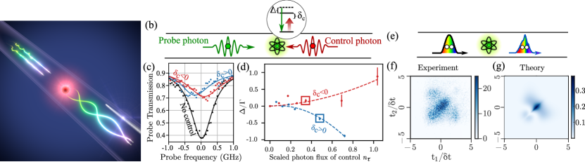
Figure 1: Observation of dynamical photon-photon interaction (color online). (a) Conceptual illustration of two-photon pulsed nonlinear interaction mediated by a quantum emitter in a nanophotonic waveguide inducing strong quantum correlations between the photon wavepackets. (b) Quantum control experiment where the interaction (transmission/reflection) of a single probe photon (green) with the quantum emitter is controlled by another photon (red). The control photon effectively shifts the emitter resonance by an amount $\Delta$ that can be controlled by the detuning of the control photon from the bare resonance $\delta_{c}$ and the control photon flux. (c) Measured transmission of the probe beam in the absence of a control photon (black curve) and with a control signal of $\delta_{c}=\omega_{c}-\omega_{0}=-0.3\Gamma$, $n_{\tau}=0.24$ (red curve) and $\delta_{c}=0.3\Gamma,$ $n_{\tau}=0.7$ (blue curve). (d) Measurement of the resonance shift $\Delta/\Gamma$ versus the scaled number of control photons for $\delta_{c}=0.3\Gamma$ (blue data) and $\delta_{c}=-0.3\Gamma$ (red data). The red and blue boxes indicate the data displayed in (c). Less than one photon suffices for inducing a pronounced shift of the resonance. The input intensity corresponds to $\approx 2$ times the saturation level. (e) Illustration of temporal quantum correlations induced by the interaction of two single photons via the quantum emitter. (f) Experimentally recorded second-order correlation function in the transmission geometry for a Gaussian pulse of duration (standard deviation) of $\delta t=340$ ps after interaction with the quantum dot. (g) Calculated second-order transmission correlation function for a two-photon pulse of duration $\delta t=340$ ps and the ideal case of a quantum emitter deterministically coupled to the waveguide without any imperfections.

The two-photon dynamics is explored in Fig. 2 by recording the two-time correlation function in transmission for different durations of the incoming pulse, $\delta t$, relative to the emitter lifetime, $\tau\approx 229$ ps (see Methods). Two interaction processes are compared, depending on the temporal separation between pulses: i) independent scattering of temporally separated single-photon pulses from the quantum dot (Fig. 2 (a)) and ii) two-photon scattering of photons originating from the same pulse (Fig. 2 (b)). Experimentally both cases can be extracted from a single series of pulsed two-photon correlation functions by analyzing data from i) subsequent pulses ($t_{2}\approx t_{1}+\Delta t$, where $\Delta t=30$ ns $\gg\tau$ is the delay between excitation pulses) or ii) same pulses ($t_{2}\approx t_{1}$). The nonlinear interaction induces temporal quantum correlations on a time scale determined by the pulse duration $\delta t$ and the lifetime $\tau.$

Case i) of independent single-photon scattering is serving as a reference measurement essentially corresponding to an uncorrelated case. The two input pulses are separated by more than lifetime, i.e. the emitter does not mediate any photon-photon interaction. The correlation measurements probe single-photon (denoted by superscript 1 on wavefunction $\Psi$) components of the scattered wavefunction, i.e. $C_{tt}^{(2)}(t_{1},t_{2})\propto|\Psi^{(1)}_{t}(t_{1})|^{2}|\Psi^{(1)}_{t}(t_{2})|^{2}$, see Fig. 2(a). The observed correlation plots can therefore be interpreted from single-photon dynamics. A short input pulse, $\delta t/\tau\lesssim 1$, is spectrally wide and has therefore a small overlap with the quantum dot bandwidth meaning that the pulse is preferentially transmitted with little effect from the emitter. Increasing the pulse duration, $\delta t/\tau\gtrsim 1$, increases the interaction with the quantum dot and thereby the probability to reflect a single photon from the incoming pulse. This reduces the probability of photon transmission (observed as a low probability amplitude around $t_{1}\sim t_{2}\sim 0$) and the overall transmission probability reduces as the pulse duration grows further.

Case ii) reveals the dynamics of two-photon (superscript 2 on wavefunction) scattering processes, i.e. $C_{tt}^{(2)}(t_{1},t_{2})\propto|\Psi_{tt}^{(2)}(t_{1},t_{2})|^{2}$. The quantum dot mediates strong photon-photon correlations tailored by the duration of the incoming pulse. For $\delta t/\tau\lesssim 1$, the pulse is spectrally wide, and only weak interaction is observed similar to case i), see data in Fig. 2(b). For longer pulses, $\delta t/\tau\gtrsim 1$, the interaction increases and we observe strong temporal correlation, i.e. the detection of one photon increases the probability of detecting another. This is observed in Fig. 2(b) as the clustering of data points around the axis $t_{1}=t_{2}$ for long pulses. The observed photon bunching in the transmission channel stems from the fact that the quantum dot can only scatter one photon at a time, and was observed previously only in continuous-wave experiments Javadi et al. (2015); Liang et al. (2018). The present experiment reveals the dynamics of this nonlinear photon-sorting process.

The temporal correlations can be quantified by performing a Schmidt decomposition of the experimental data $C^{(2)}_{tt}(t_{1},t_{2})$ Zielnicki et al. (2018); Law et al. (2000) (see Methods for details). From the Schmidt coefficients $\lambda_{i}$ we extract the degree of temporal correlation $T_{c}=1-\sum_{i}\lambda_{i}^{4}$ versus pulse duration $\delta t/\tau$, see Fig.2(c). Case i) of independent scattering does not introduce any significant correlations, $T_{c}\simeq 0$, which is the case for a separable quantum state. A fundamentally different behavior is observed for the two-photon scattering case of ii) where $T_{c}$ is found to grow with pulse duration. This behavior is a manifestation of the observed correlated photon-pair emission (see Fig.2(b)) resembling nonlinear parametric down-conversion or four-wave mixing sourcesKuzucu et al. (2008). In the present implementation, a single quantum dot deterministically coupled to a waveguide acts as the photon-pair source.

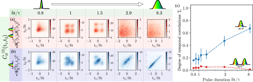
Figure 2: Temporal quantum correlations due to photon-photon dynamical interaction in the transmission channel (color online). Measured time-resolved second-order correlation function for various pulse duration $\delta t$ relative to the quantum dot lifetime $\tau$ and for (a) two single photons from subsequently scattered pulses and (b) two photons contained in the same pulse. (c) Extracted degree of temporal correlation $T_{c}$ versus pulse duration for the two data sets (a) [red] and (b) [blue].

The WQED photon-photon nonlinear interaction has unique features due to an intricate interplay between the drive pulse and the field scattered by the quantum dot. The resulting quantum interference is studied by recording $C^{(2)}_{\mu\mu^{\prime}}(t_{1},t_{2})$ for reflection or transmission channels $\mu,\mu^{\prime}=t,r$ in the waveguide, see Fig. 3(a)-(c) for both one- and two-photon cases. In the forward propagating direction (transmission channel) quantum interference is present, while in the backward direction (reflection channel) solely the scattering response of the quantum dot is observed. Furthermore, the cross-correlation between reflection/transmission channels is also studied. Line-cuts through the two-dimensional correlation plots are presented both versus the sum of the detection times (Fig. 3(d)-(f)) and versus the delay (Fig. 3(g)-(i)) comparing both the one-photon and two-photon responses. These data sets are instructive for the physical interpretation of the quantum dynamics. Three different regimes are defined corresponding to: 1) excitation, 2) saturation and stimulated emission, and 3) spontaneous emission of the emitter.

In regime 1), the polarization of the emitter builds up due to the rise of the excitation pulse. Here the one- and two-photon dynamics is similar since the probability of absorption and remains small. The build up of the excitation probability is directly revealed in the reflection data (Fig. 3 (e)), since no interference with the incoming pulse occurs in this case.

As the excitation probability becomes sizable, we enter regime 2) of stimulated emission and saturation where stark differences between one- and two-photon dynamics are observed. The reflection is strongly suppressed in the two-photon case (Fig. 3 (e)), which is a direct consequence of the emitter only reflecting one photon at a time also leading to the dip in the time delay data in Fig. 3 (h). The single-photon response is dominated by a strong reflection, a testimony of the efficient coupling of the emitter to the waveguide leading to a large optical extinction, which is confirmed by the suppression of transmission-transmission and transmission-reflection events in Fig. 3 (d) and (f), respectively. In contrast, a pronounced enhancement is found for the two-photon dynamics since a single photon suffices for saturating the emitter enabling the transmission of a second photon. The time delay data in Fig. 3 (g) and (i) allows to further discern the dynamics of this process. The strong asymmetry in the transmission-reflection data (Fig. 3 (i)) reveals the temporal ordering of the process, where a photon is first absorbed, then a second photon is transmitted and finally the first photon is re-emitted. In the transmission-transmission channel, the two detected photons had propagated in the same direction enabling stimulated emission. We observe a pronounced preference for for two-photon transmission compared to the single-photon case, see Fig. 3 (d). We further monitor the delay between the transmitted photons, and find an increased emission rate in the forward (transmission) direction by comparing the time delay data in Fig. 3 (g) to the transmission-reflection data in Fig. 3 (i). These observations are signatures of stimulated emission of a saturable emitter occurring here in the most fundamental setting of just two quanta of light and mediated by a single quantum emitter. Indeed with the efficient and coherent photon-emitter coupling in the photonic-crystal waveguide even a single photon pulse suffices for stimulating emission.

Finally, after the excitation pulse has passed, the system enters into regime 3) where the remaining population of the emitter decays by spontaneous emission. We observe that generally the two-photon response is suppressed relative to the one-photon response reflecting the fact that the single emitter only stored one excitation.

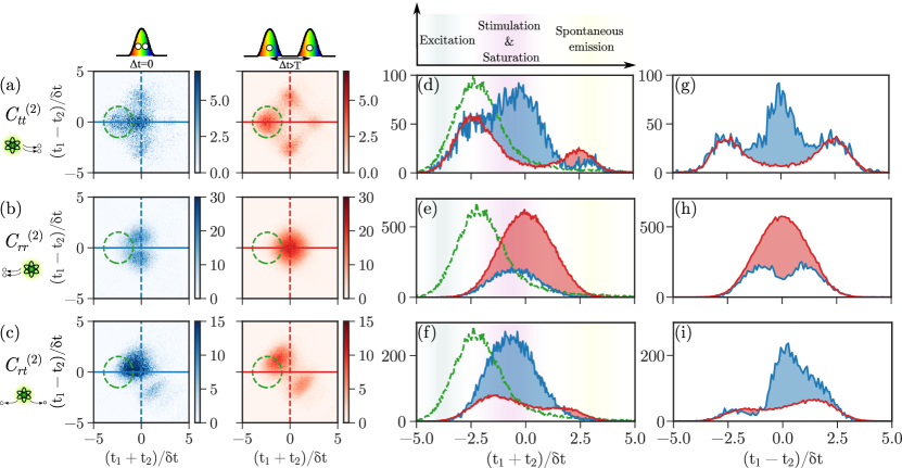
Figure 3: Unravelling the physical processes behind the quantum dynamics (color online). Experimental measurements of the two-photon correlation function for $\delta t/\tau=1.5$ and photons detected in different spatial modes i.e. both photons being transmitted (a), reflected (b), or one photon reflected and the other transmitted (c) by the quantum dot. The two different cases correspond to two photons in the same pulse (blue data) or one photon in each subsequent pulse (red data). The green dashed line marks the position of the incident pulse used to excite the quantum dot. (d)-(f) Line cuts at $t_{1}=t_{2}$, indicated by the full line in the correlation data in (a)-(c), as a function of $t_{1}+t_{2}$ for the three cases. The main physical processes responsible for the dynamics in the various temporal domains are noted.(g)-(i) Line cuts at $t_{1}=-t_{2}$, indicated by the dashed line in the correlation data in (a)-(c) as a function of $t_{1}-t_{2}$ for the three cases. To increase the signal-to-noise ratio of the line cuts, the coincidence counts have been integrated over 10 bins (corresponding to 200 ps).

Using a quantum dot deterministically coupled to a nanophotonic waveguide, we have reported two fundamental demonstrations of quantum nonlinear optics: a single-photon pump-probe experiment where one photon controls another and a quantum-pulse experiment where photon-emitter dynamic scattering was discerned into its most fundamental constituents. The current focus was to unravel the underlying physical processes behind quantum nonlinear interaction with quantum pulses, however applications are foreseen. For instance, photon sorters have been proposed as a basis for a deterministic Bell analyzer for photons Witthaut et al. (2012), which is a key enabling component in photonic quantum-information processing. Another interesting direction is to exploit and tailor the nonlinear interaction to synthesize specific photonic quantum states Kiilerich and Mølmer (2019), possibly boosted in a quantum optics neural network Steinbrecher et al. (2019). Hybrid discrete-continuous variable architectures for photonic quantum computing appear another promising future research direction, since the nonlinear response of the emitter could provide a non-Gaussian photonic operation, which is currently the ”missing link” in continuous-variable quantum-information processing.

We thank Klaus Mølmer and Ravitej Uppu for valuable discussions. We acknowledge funding from the Danish National Research Foundation (Center of Excellence “Hy-Q,” grant number DNRF139). This project has received funding from the European Union’s Horizon 2020 research and innovation programme under grant agreement No. 824140 (TOCHA, H2020-FETPROACT-01-2018).

I Methods

I.1 Photon-emitter interface

The considered quantum emitter is a neutral excitonic state of a self-assembled InGaAs quantum dot (QD). The emitter is embedded in a GaAs suspended photonic-crystal waveguide and includes doped layers to form a p-i-n diode heterostructure, which enables electrical contacting allowing charge stabilization of the environment and tuning of the resonance through the DC Stark effect. Details about the sample can be found in Ref Kiršanskė et al. (2017). The sample is cooled down to $4~{}$K to reduce phonon-induced dephasing. The transition decay rate has been measured through p-shell excitation to be $4.364(5)~{}$ns^-1, corresponding to a measured lifetime of $\tau\simeq 229~{}$ps. For comparison, the linewidth of the transition is measured to be $755~{}$ MHz.

I.2 Two-color photon control experiment

I.2.1 Experimental setup

In the experiment realizing two-photon control, see data in Fig. 1(c)+(d) of the main manuscript, two tunable continuous-wave (CW) lasers (linewidth $<10~{}$kHz) were applied for the probe and control laser that excited the QD through the two gratings of the nanophotonic waveguide, see sketch in Fig. 4. By using a combination of polarisation optimization and careful alignment, the transmission of the probe signal was recorded, with an extinction ratio between the laser excitation and the signal of $\approx 15$.

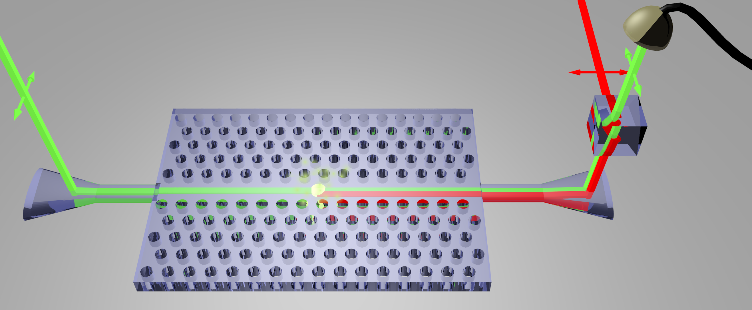
Figure 4: Experimental setup for the two-color photon control experiment. The probe (green) and control (red) CW weak lasers of orthogonal polarizations are sent through the waveguide by using opposite gratings. The transmission of the probe signal can be recorded with single photon detectors.

I.2.2 Calibration of the control photon flux

To determine the number of photons required to switch the QD, we first calibrate the control laser power in the waveguide by recording a saturation measurement of the QD. The fluorescence intensity spectrum $I_{R}$ reflected by the QD is measured as a function the QD-laser detuning $\Delta$ and laser power $P$, see data in Fig. 5(a). The counts $I_{R}$ are corrected for background and the spectra are fitted using the formulas derived in Ref. Le Jeannic et al. (2021). For modelling the data, we used the following set of parameters: $\beta\approx 0.9$, dephasing rate $\Gamma_{0}\approx 0.3$ ns^-1, and the calibrating parameter $\alpha\approx 0.3$ ns${}^{-2}/\mu W$ relates the Rabi frequency $\Omega$ to the laser power through $\Omega=\sqrt{\alpha P}$. The decay rate of the emitter was independently measured to be $\Gamma_{\text{tot}}=4.364(5)$ ns^-1.

The critical photon flux during one lifetime of the control beam is then calculated to be: $n_{c}=(1+2\Gamma_{0}/\Gamma_{\text{tot}})^{2}/4\beta^{2}$, which for our system was determined to be $n_{c}\approx 0.42$Javadi et al. (2015); Thyrrestrup et al. (2018). We can finally calibrate the scaled photon flux of the control beam $n_{\tau}$ by using: $n_{\tau}=Sn_{c}$, where the saturation parameter is then given by $S=8\Omega^{2}/(\Gamma_{\text{tot}}(2\Gamma_{0}+\Gamma_{\text{tot}}))$ As a sanity check, we can compare the measured $I_{R}$ against the analytic form of the saturation curve at resonance: $I_{R}=a\beta^{2}\Gamma_{\text{tot}}^{2}/(8S)$, which is shown in Fig. 5(b).

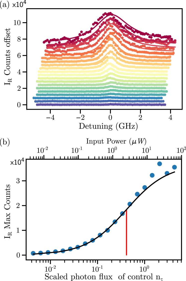
Figure 5: Calibration of photon flux. (a) Fluorescence measured in reflection (points) and corresponding fit to theory as a function of laser power (going from low (blue) to high (red) power) versus detuning. Fits are shown with solid lines and the fluorescence is offset as a function of laser power for clarity. (b) The measured intensity $I_{R}$ as a function of scaled photon flux for measured data (points) alongside the theoretical curve. Error bars due to Poissonian counts are smaller than the point size. The critical photon number $n_{c}\approx 0.42$ is marked, demonstrating that an efficient optical nonlinearity with single-photon sensitivity is achieved.

I.2.3 Extracting the nonlinear resonance shift

To calculate the nonlinear resonance shift, the control beam is detuned $\pm 200$ MHz relative to the QD, the probe beam is scanned across the QD and the transmission measured as a function of control laser power. The control beam naturally induces a power-dependent frequency shift, always towards longer wavelengths in the QD due to thermal effects and carrier creation. To account for this, and to isolate the true multi-color nonlinear effect, we pre-characterize the power dependent frequency shift of the control laser before each measurement. Fig. 6 shows an example of the measured QD frequency shift versus control laser power constituting a calibration curve. We then apply a power dependent frequency correction to the control beam to maintain the QD-control beam detuning, effectively ‘tracking’ the QD as a function of power. The probe beam transmissions are then fitted by a Lorentzian function to estimate the central frequency, which is plotted as a function of photon flux in Fig. 1(d). A second order polynomial is fitted to the photon number versus normalised frequency shift. From this we can determine the photon flux required to shift the QD by a full linewidth $\Delta/\Gamma_{\text{tot}}=-1$, when the control beam is detuned by $200$ MHz relative to the resonance. We find $0.97\pm 0.27$ photons within the emitter lifetime shift the QD by a full linewidth. This corresponds to a saturation parameter of $S=n_{\tau}/n_{c}\approx 2.3$.

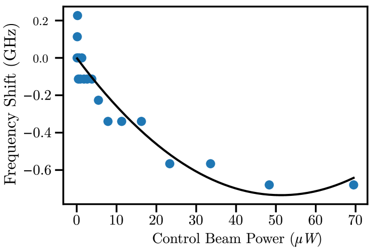
Figure 6: Frequency calibration measurements. The shift in the resonance frequency of the fluorescence of the QD as a function of control laser power (blue points), fitted to a second order polynomial (black line).

I.3 Dynamics of two photons interacting with a quantum emitter

I.3.1 Experimental setup

In the second experiment, the temporal photon-photon dynamics is probed. Here a CW laser (linewidth $<10~{}$kHz) is sent to a $20$ GHz electro-optical modulator (iXBlue NIR-MX800-LN-20) to generate tunable pulses with duration between 300 ps and 10 ns. Furthermore, 100 ps pulses are generated using another pulse generator (Alnair EPG-210 picosecond electrical pulse generator) and an external clock. The repetition rate of the experiment is set to $33~{}$MHz, enabling time delay between the pulses much longer than the emitter’s response time. The laser central wavelength is tuned to the resonance of the exciton and is strongly attenuated to contain an average photon number below $0.1$ photons within the lifetime of the emitter. Two-photon correlation measurements are performed in the different propagation directions of the light, following the same scheme as detailed in Ref Le Jeannic et al. (2021) for CW-excitation. The coincidence events are detected with four superconducting nanowire single photon detectors (SNSPD) with timing jitters below $30$ ps in transmission, and below $150$ ps in reflection, and using a Swabian ultra time tagger. To avoid issues related to the accumulation of jitter over long time acquisition, the clock signal of the laser is also registered, and single photon time detection events are registered according to this clock signal.

We are able to access in a single measurement run both the correlation data originating from one-photon and two-photon interactions. This is done by recording the second-order intensity correlation function $G^{(2)}_{xy}(t_{1},t_{2})$ with two single-photon detectors in a pulsed experiment. By recording two-photon detection events where $t_{1}\approx t_{2}$ and $t_{1}\approx t_{2}+\Delta t$, respectively, we post-select on the processes where two photons from the same excitation pulse or two subsequent excitation pulses were interacting with the QD. $\Delta t$ is the separation between excitation pulses.

I.3.2 Temporal Correlations

A standard way of estimating entanglement in a bipartite system $\ket{\psi}_{A,B}=\sum_{i}\lambda_{i}\ket{i}_{A}\ket{i}_{B}$ is via the purity of the reduced density matrix $\Tr(\rho_{A}^{2})=\sum_{i}\lambda_{i}^{4}$. For a maximally entangled state $\Tr(\rho_{A}^{2})=1/N$ (where $N$ is the dimension of $\rho_{A}$), while for a separable state $\Tr(\rho_{A}^{2})=1$. While we do not have experimental access to the phase information from $C^{(2)}_{tt}(t_{1},t_{2})$, we can instead quantify the temporal intensity correlation, which introduces a bound on the purity.

To extract the temporal correlations of the time-resolved coincidence counts $C^{(2)}_{tt}(t_{1},t_{2})$ in Fig. 2, we do a Schmidt decomposition of the matrix containing the square root of the count rates $C^{\prime}_{jl}=\sqrt{C^{(2)}_{tt}(d_{t}j,d_{t}l)}$, where $d_{t}$ the time bin size. We perform a singular value decomposition of $C^{\prime}$, obtaining $C^{\prime}=\sum_{i}\lambda_{i}v_{i}u_{i}^{\dagger}$ with $\lambda_{i}$ the singular values of $C^{\prime}$ (normalized as $\sum_{i}\lambda_{i}^{2}=1$) and $u_{i}$, $v_{i}$ unitary matrices. We then use the obtained singular values $\lambda_{i}$ to estimate the temporal correlation of $C^{\prime}$ via the quantity $T_{c}=1-\sum_{i}\lambda_{i}^{4}$ defined in the main text Zielnicki et al. (2018); Fang et al. (2014). This quantifies the degree of temporal correlations in $C^{(2)}_{tt}(t_{1},t_{2})$ such that $T_{c}\sim 0$ implies the uncorrelated case (the matrix can be factorized $C^{\prime}_{jl}=|\Psi^{(1)}_{t}(d_{t}j)||\Psi^{(1)}_{t}(d_{t}l)|$) and $T_{c}\sim 1$ corresponds the maximally correlated case.

In practice, the value of $T_{c}$ is sensitive to the time bin size $d_{t}$. To enable a fair comparison between data sets of different pulse widths, we must therefore vary $d_{t}$ independently for each data set. To do this, for each data set $C^{(2)}_{tt}$ we calculate the maximum count value in any bin $c_{\text{max}}$ and then take the mean across all data sets $\bar{c}_{\text{max}}$ to give a target count value. For each data set we then increase $d_{t}$ until there is at least a single element of $C^{(2)}_{tt}$ with a count value greater than $\bar{c}_{\text{max}}$. We repeat this analysis independently for the data of the correlated ($\Delta t\sim 0$) and uncorrelated scattering ($\Delta t\gg\tau$), for which we have $C^{\prime}_{jl}\approx|\Psi^{(2)}_{tt}(d_{t}j,d_{t}l)|+{\cal O}(|\alpha|^{2})$ and $C^{\prime}_{jl}\approx|\Psi^{(1)}_{t}(d_{t}j)||\Psi^{(1)}_{t}(d_{t}l)|+{\cal O}(|\alpha|^{2})$, respectively. Error bars are estimated by performing a Monte Carlo analysis on the entire data processing pipeline, assuming Poissonian distributed count rates.

References

- Kimble (2008) H. J. Kimble, Nature 453, 1023 (2008).
- Wang et al. (2020) J. Wang, F. Sciarrino, A. Laing, and M. G. Thompson, Nat. Photonics 14, 273 (2020).
- Uppu et al. (2021) R. Uppu, L. Midolo, X. Zhou, J. Carolan, and P. Lodahl, Nat. Nanotechnol. , 1 (2021).
- Lindner and Rudolph (2009) N. H. Lindner and T. Rudolph, Phys. Rev. Lett. 103, 113602 (2009).
- Chang et al. (2014) D. E. Chang, V. Vuletić, and M. D. Lukin, Nat. Photonics 8, 685 (2014).
- Chang et al. (2018) D. E. Chang, J. S. Douglas, A. González-Tudela, C.-L. Hung, and H. J. Kimble, Rev. Mod. Phys. 90, 031002 (2018).
- Haroche and Raimond (2006) S. Haroche and J. M. Raimond, Exploring the Quantum: Atoms, Cavities, and Photons (Oxford Univ. Press, 2006).
- Kimble et al. (1977) H. J. Kimble, M. Dagenais, and L. Mandel, Phys. Rev. Lett. 39, 691 (1977).
- Kuhn et al. (2002) A. Kuhn, M. Hennrich, and G. Rempe, Phys. Rev. Lett. 89, 067901 (2002).
- Duan and Kimble (2004) L.-M. Duan and H. J. Kimble, Phys. Rev. Lett. 92, 127902 (2004).
- Reiserer et al. (2014) A. Reiserer, N. Kalb, G. Rempe, and S. Ritter, Nature 508, 237 (2014).
- Jaynes and Cummings (1963) E. T. Jaynes and F. W. Cummings, Proc. IEEE 51, 89 (1963).
- Lund-Hansen et al. (2008) T. Lund-Hansen, S. Stobbe, B. Julsgaard, H. Thyrrestrup, T. Sünner, M. Kamp, A. Forchel, and P. Lodahl, Phys. Rev. Lett. 101, 113903 (2008).
- Chang et al. (2007) D. E. Chang, A. S. Sørensen, E. A. Demler, and M. D. Lukin, Nat. Phys. 3, 807 (2007).
- Vetsch et al. (2010) E. Vetsch, D. Reitz, G. Sagué, R. Schmidt, S. T. Dawkins, and A. Rauschenbeutel, Phys. Rev. Lett. 104, 203603 (2010).
- Tey et al. (2008) M. K. Tey, Z. Chen, S. A. Aljunid, B. Chng, F. Huber, G. Maslennikov, and C. Kurtsiefer, Nat. Phys. 4, 924 (2008).
- Lang et al. (2011) C. Lang, D. Bozyigit, C. Eichler, L. Steffen, J. M. Fink, A. A. Abdumalikov, M. Baur, S. Filipp, M. P. da Silva, A. Blais, and A. Wallraff, Phys. Rev. Lett. 106, 243601 (2011).
- Deppe et al. (2008) F. Deppe, M. Mariantoni, E. P. Menzel, A. Marx, S. Saito, K. Kakuyanagi, H. Tanaka, T. Meno, K. Semba, H. Takayanagi, E. Solano, and R. Gross, Nat. Phys. 4, 686 (2008).
- Goban et al. (2014) A. Goban, C.-L. Hung, S.-P. Yu, J. D. Hood, J. A. Muniz, J. H. Lee, M. J. Martin, A. C. McClung, K. S. Choi, D. E. Chang, O. Painter, and H. J. Kimble, Nat. Commun. 5, 1 (2014).
- Peyronel et al. (2012) T. Peyronel, O. Firstenberg, Q.-Y. Liang, S. Hofferberth, A. V. Gorshkov, T. Pohl, M. D. Lukin, and V. Vuletic, Nature 488, 57 (2012).
- Lodahl et al. (2015) P. Lodahl, S. Mahmoodian, and S. Stobbe, Rev. Mod. Phys. 87, 347 (2015).
- Lodahl et al. (2017) P. Lodahl, S. Mahmoodian, S. Stobbe, A. Rauschenbeutel, P. Schneeweiss, J. Volz, H. Pichler, and P. Zoller, Nature 541, 473 (2017).
- Barik et al. (2018) S. Barik, A. Karasahin, C. Flower, T. Cai, H. Miyake, W. DeGottardi, M. Hafezi, and E. Waks, Science 359, 666 (2018).
- Asenjo-Garcia et al. (2017) A. Asenjo-Garcia, M. Moreno-Cardoner, A. Albrecht, H. J. Kimble, and D. E. Chang, Phys. Rev. X 7, 031024 (2017).
- Kiilerich and Mølmer (2019) A. H. Kiilerich and K. Mølmer, Phys. Rev. Lett. 123, 123604 (2019).
- Fan et al. (2010) S. Fan, i. m. c. E. Kocabaş, and J.-T. Shen, Phys. Rev. A 82, 063821 (2010).
- Shen and Fan (2007) J.-T. Shen and S. Fan, Phys. Rev. Lett. 98, 153003 (2007).
- Mahmoodian et al. (2020) S. Mahmoodian, G. Calajó, D. E. Chang, K. Hammerer, and A. S. Sørensen, Phys. Rev. X 10, 031011 (2020).
- Rephaeli and Fan (2012) E. Rephaeli and S. Fan, Phys. Rev. Lett. 108, 143602 (2012).
- Wu et al. (1977) F. Y. Wu, S. Ezekiel, M. Ducloy, and B. R. Mollow, Phys. Rev. Lett. 38, 1077 (1977).
- Sipahigil et al. (2016) A. Sipahigil, R. E. Evans, D. D. Sukachev, M. J. Burek, J. Borregaard, M. K. Bhaskar, C. T. Nguyen, J. L. Pacheco, H. A. Atikian, C. Meuwly, R. M. Camacho, F. Jelezko, E. Bielejec, H. Park, M. Lončar, and M. D. Lukin, Science 354, 847 (2016).
- Maser et al. (2016) A. Maser, B. Gmeiner, T. Utikal, S. Götzinger, and V. Sandoghdar, Nat. Photonics 10, 450 (2016).
- Javadi et al. (2015) A. Javadi, I. Söllner, M. Arcari, S. L. Hansen, L. Midolo, S. Mahmoodian, G. Kirsanske, T. Pregnolato, E. H. Lee, J. D. Song, S. Stobbe, and P. Lodahl, Nature Communications 6, 8655 (2015).
- Mirhosseini et al. (2019) M. Mirhosseini, E. Kim, X. Zhang, A. Sipahigil, P. B. Dieterle, A. J. Keller, A. Asenjo-Garcia, D. E. Chang, and O. Painter, Nature 569, 692 (2019).
- Shen et al. (2017) Y. Shen, N. C. Harris, S. Skirlo, M. Prabhu, T. Baehr-Jones, M. Hochberg, X. Sun, S. Zhao, H. Larochelle, D. Englund, and M. Soljačić, Nat. Photonics 11, 441 (2017).
- Ramos and García-Ripoll (2017) T. Ramos and J. J. García-Ripoll, Phys. Rev. Lett. 119, 153601 (2017).
- Le Jeannic et al. (2021) H. Le Jeannic, T. Ramos, S. F. Simonsen, T. Pregnolato, Z. Liu, R. Schott, A. D. Wieck, A. Ludwig, N. Rotenberg, J. J. García-Ripoll, and P. Lodahl, Phys. Rev. Lett. 126, 023603 (2021).
- Heuck et al. (2020) M. Heuck, K. Jacobs, and D. R. Englund, Phys. Rev. Lett. 124, 160501 (2020).
- Liang et al. (2018) Q.-Y. Liang, A. V. Venkatramani, S. H. Cantu, T. L. Nicholson, M. J. Gullans, A. V. Gorshkov, J. D. Thompson, C. Chin, M. D. Lukin, and V. Vuletić, Science 359, 783 (2018).
- Zielnicki et al. (2018) K. Zielnicki, K. Garay-Palmett, D. Cruz-Delgado, H. Cruz-Ramirez, M. F. O’Boyle, B. Fang, V. O. Lorenz, A. B. U’Ren, and P. G. Kwiat, Journal of Modern Optics 65, 1141 (2018).
- Law et al. (2000) C. K. Law, I. A. Walmsley, and J. H. Eberly, Phys. Rev. Lett. 84, 5304 (2000).
- Kuzucu et al. (2008) O. Kuzucu, F. N. C. Wong, S. Kurimura, and S. Tovstonog, Phys. Rev. Lett. 101, 153602 (2008).
- Witthaut et al. (2012) D. Witthaut, M. D. Lukin, and A. S. Sørensen, EPL (Europhysics Letters) 97, 50007 (2012).
- Steinbrecher et al. (2019) G. R. Steinbrecher, J. P. Olson, D. Englund, and J. Carolan, npj Quantum Inf. 5, 1 (2019).
- Kiršanskė et al. (2017) G. Kiršanskė, H. Thyrrestrup, R. S. Daveau, C. L. Dreeßen, T. Pregnolato, L. Midolo, P. Tighineanu, A. Javadi, S. Stobbe, R. Schott, A. Ludwig, A. D. Wieck, S. I. Park, J. D. Song, A. V. Kuhlmann, I. Söllner, M. C. Löbl, R. J. Warburton, and P. Lodahl, Phys. Rev. B 96, 165306 (2017).
- Thyrrestrup et al. (2018) H. Thyrrestrup, G. Kirsanske, H. Le Jeannic, T. Pregnolato, L. Zhai, L. Raahauge, L. Midolo, N. Rotenberg, A. Javadi, R. Schott, A. D. Wieck, A. Ludwig, M. C. Löbl, I. Söllner, R. J. Warburton, and P. Lodahl, Nano Letters 18, 1801 (2018).
- Fang et al. (2014) B. Fang, O. Cohen, M. Liscidini, J. E. Sipe, and V. O. Lorenz, Optica 1, 281 (2014).