Hubble tension and $n_{s}$.– The Hubble constant ($H_{0}$) inferred from the $\Lambda$CDM model with the input of the temperature/polarization anisotropies of the cosmic microwave background (CMB) is [1]

$$H_{0}^{\rm CMB}=67.4\pm 0.5{\rm\leavevmode\nobreak\ km\leavevmode\nobreak\ s^{-1}\leavevmode\nobreak\ Mpc^{-1}}.$$ (1)

This is known to differ from the locally measured value at low red shifts [2, 3, 4, 5, 6] by at least $4\sigma$ level (see reviews  [7, 8, 9, 10].) Recently, the SH0ES Team has reported a new result from the measurement of 42 SNe la at $z<0.01$, in which [11]

$$H_{0}=73.04\pm 1.04{\rm\leavevmode\nobreak\ km\leavevmode\nobreak\ s^{-1}\leavevmode\nobreak\ Mpc^{-1}}.$$ (2)

Thus the long-standing discrepancy is further strengthened and the new result shows an around $5\sigma$ difference from the $\Lambda$CDM prediction.

There have been proposed many models altering the cosmology around or after the recombination era to relax the Hubble tension (see e.g. [10] and the references therein). In particular, some of them require different initial conditions for the very early Universe from the $\Lambda$CDM model. For instance, the primordial curvature perturbation is given in the form of

$${\cal P}_{\zeta}[k]={\cal P}_{\zeta}[k_{*}](k/k_{*})^{n_{s}-1}.$$ (3)

where the index $*$ denotes the variable evaluated at the horizon exit of the CMB scales here and hereafter, and $n_{s}$ is the scalar spectral index. In various solutions to the Hubble tension, $n_{s}$ is often diffenrent from the $\Lambda$CDM value,

$$n_{s}\neq n_{s}^{\rm\Lambda CDM}$$ (4)

with $n^{\Lambda\rm CDM}_{s}=0.965\pm 0.004$ [1]. Intriguingly, in the light of the Hubble tension $n_{s}=1$, is not ruled out [12, 13].

Moreover, certain promising scenarios predict a relative suppression of the small scale fluctuations. This can be compensated by increasing $n_{s}$. Then, $n_{s}>n_{s}^{\Lambda\rm CDM}$ is even favored. For instance, in the early dark energy scenario and its modifications [14, 15, 16, 17, 18, 19, 20, 21], an enhanced early integrated Sachs-Wolfe effect suppresses the growth of perturbations which leads to a larger $n_{s}$ and a higher density of cold dark matter [13, 22].. Another example is the ${\rm\,eV}$ scale majoron which was proposed to explain the Hubble tension [28]. The hot majoron around the recombination era seems to suppress the small scale structure which gives a preference to $n_{s}>n_{s}^{\rm\Lambda CDM}$ from the $\Lambda$CDM value. There are some other solutions to the Hubble tension which also have the best fit of $n_{s}\approx 1$ e.g. [17, 19, 20, 28].

Given those observations and the strengthened significance of the Hubble tension, it may be a good point to discuss their implications for the very early Universe. In this Letter, we discuss some simple cosmological models to increase or decrease $n_{s}$ than the $\Lambda$CDM value. In particular, we will mainly focus on the $n_{s}\approx 1$ cosmology which may be preferred from various scenarios for explaining the Hubble tension.

Inflation with $n_{s}\approx 1$.– The slow-roll inflation solves various fine-tuning problems associated with the initial condition of the big-bang cosmology. More importantly, the quantum fluctuations of the inflaton are known to generate the density perturbations. The predicted scalar spectral index in the simple slow-roll inflation models is

$$n_{s}-1\simeq-6\varepsilon+2\eta,$$ (5)

where $\varepsilon$ and $\eta$ are the slow-roll parameters of the inflaton. Since $n_{s}$ depends on the functional form of the inflaton potential as well as thermal history after inflation, it is often used to constrain inflation models. On the other hand, $n_{s}$ is known to be rather sensitive to tiny corrections to the inflaton potential, especially in the so-called small-field inflation. For instance, the predicted $n_{s}$ is smaller than $n^{\Lambda\rm CDM}_{s}$ in the quartic hilltop inflation, but it can be easily enhanced close to or even larger than $n^{\Lambda\rm CDM}_{s}$ by introducing a tiny linear term [32]. In many inflation models which predict $n_{s}<1$ in their original set-up, it is similarly possible to add some modifications to the inflaton potential to realize $n_{s}\approx 1$. This is an interesting direction to study. However, here we instead pursue a scenario that generically predicts $n_{s}\approx 1$ over wider parameter space.

Review on curvaton.– Let us briefly review the curvaton scenario [33, 34, 35, 36] in which the curvature perturbation is generated by the fluctuation of a curvaton field $\sigma$ during inflation rather than the inflaton fluctuation. We assume that $\sigma$ does not have a significant interaction to the inflaton, nor a non-minimal coupling to gravity. Let us decompose the curvaton field into the spatially homogeneous part and a fluctuation about it, $\sigma[\vec{x}]=\sigma_{0}+\delta\sigma[\vec{x}]$, and denote the Fourier component of the perturbation as $\delta\sigma_{\vec{k}}$, where the time dependence is not shown explicitly. The fluctuation evolves following

$$\delta\ddot{\sigma}_{\vec{k}}+3H\delta\dot{\sigma}_{\vec{k}}+((k/a)^{2}+V^{\prime\prime})\delta\sigma_{\vec{k}}=0,$$ (6)

where $a$ is the scale factor, $H$ is the Hubble parameter, $V=V[\sigma]$ is the curvaton potential, and the prime denotes the derivative with respect to the variable of the function. When $|V^{\prime\prime}|\lesssim H^{2}_{*}$, the fluctuation of the curvaton generated during inflation is given by

$$(\delta\sigma_{\vec{k}})^{2}\simeq\left(\frac{H_{*}}{2\pi}\right)^{2}(k/k_{*})^{(n_{\sigma}-1)}$$ (7)

with

$$n_{\sigma}-1=\left(2\frac{\dot{H}}{H^{2}}+\frac{2}{3}\frac{V^{\prime\prime}}{H^{2}}\right)_{*}.$$ (8)

In the slow-roll inflation, $\dot{H}/H^{2}$ can be sizable only for inflation models with super-Planckian field excursion, and such inflation models are often assumed to realize $n_{s}<1$ in the context of curvaton scenario. However, a super-Planckian field excursion is known to be in tension with the quantum gravity. Thus, in the following we neglect the first term, and focus on the second term in the parenthesis.

The curvaton $\sigma$ starts to oscillate when the mass becomes comparable to the Hubble parameter after inflation. The perturbation in the energy density is obtained as

$$\frac{\delta\rho_{\sigma}}{\rho_{\sigma}}\approx\frac{\sqrt{(\delta\sigma_{\vec{k}})^{2}}}{\sigma_{0}}\simeq\frac{2H_{*}}{2\pi\sigma_{0}}$$ (9)

by assuming $H_{*}\ll\sigma_{0}$, and $V\propto\sigma^{2}$ at the onset of the oscillation. We assume that the curvaton subsequently dominates over the Universe and it later decays to the standard model (SM) particles it couples to. The curvaton decay reheats the Universe and the SM particles make up the thermal bath of the big-bang cosmology. Then, the density perturbation of the plasma follows that of the curvaton,

$${\cal P}_{\zeta}\approx\left(\frac{H_{*}}{\pi\sigma_{0}}\right)^{2},\leavevmode\nobreak\ \leavevmode\nobreak\ n_{s}\approx\left.1+\frac{2}{3}\frac{V^{\prime\prime}}{H^{2}}\right|_{*}.$$ (10)

Since the CMB normalization gives [38]

$${\cal P}_{\zeta}\approx 2\times 10^{-9},$$ (11)

we obtain

$$H_{*}\approx 1.4\times 10^{12}{\rm\,GeV}\left(\frac{\sigma_{0}}{10^{16}{\rm\,GeV}}\right).$$ (12)

A bound on $H_{*}$ is derived from the tensor-to-scalar ratio [39]

$$r\equiv{\cal P}_{h}/{\cal P}_{\zeta}<0.036$$ (13)

which together with Eq. (11) gives an upper limit on the tensor mode. This bound leads to

$$H_{*}\lesssim 4.7\times 10^{13}\,{\rm\,GeV}.$$ (14)

This upper bound on the inflation scale with the CMB normalization implies that the homogeneous part of the curvaton field, $\sigma_{0}$, is sub-Planckian. We emphasize that in our scenario the inflation is not required to explain the density perturbation and it is quite easy to build such models. Thus in the following, we do not specify an inflation model, and only require that the inflaton field excursion is sub-Planckian.

In the context of curvaton, one often considers a sizable tachyonic mass $\sqrt{|V^{\prime\prime}|}\sim 0.1H_{*}$ to explain $n_{s}=n_{s}^{\rm\Lambda CDM}<1$. However, in this case, the curvaton starts to oscillate soon after inflation, and it is difficult to dominate the Universe unless the initial position is close to the top of the potential [37, 40]. Also, in this case, the non-Gaussianity is known to be logarithmically enhanced. If we allow the curvaton potential to be time-dependent, a natural way may be to introduce a non-minimal coupling of ${\cal L}\supset\xi\sigma^{2}R$ with $|\xi|={\cal O}(0.01)$ and then $V^{\prime\prime}$ in the Einstein frame gets a contribution of $\mathcal{O}(\xi H_{*}^{2})$.

Curvaton scenarios in light of Hubble tension.– As we mentioned, in this Letter we focus on $n_{s}\approx 1$. This implies that, in the context of a curvaton scenario,

$$|(V^{\prime\prime})_{*}|\ll H^{2}_{*}$$ (15)

for which $n_{s}\approx 1$ is naturally realized. The small curvature of the potential also means the suppression in the non-minimal coupling. From the viewpoint of naturalness, the suppression may imply symmetry, e.g. supersymmetry or shift symmetry. In the following, we consider the latter to suppress the curvaton mass.

ALP as curvaton.– An interesting possibility is that the curvaton is an axion [34, 41, 40]. In this case the potential naturally has the form of

$$V=\Lambda^{4}(1-\cos[\sigma/f_{a}])$$ (16)

where $\Lambda$ is a dynamical scale that breaks the “Peccei-Quinn” symmetry, and $f_{a}$ is the decay constant. We assume $\Lambda$ does not depend on the cosmic time. The mass, $m_{a}$, of the axion is obtained as

$$m_{a}=\frac{\Lambda^{2}}{f_{a}}.$$ (17)

For successful reheating, we need to couple the axion to the SM particles. In particular, an axion coupled to photons is called an axion-like-particle (ALP). The ALP coupling to a pair of photons is given by

$${\cal L}=c_{\gamma}\frac{\alpha}{4\pi}\frac{\sigma}{f_{a}}F_{\mu\nu}\tilde{F}^{\mu\nu}$$ (18)

where $c_{\gamma}$ is the anomaly coefficient, $\alpha$ the fine-structure constant, and $F_{\mu\nu}$ ($\tilde{F}_{\mu\nu}$) the photon field strength (its dual), Then the axion or ALP can decay into a photon pair with a decay rate of

$$\Gamma_{\rm dec,\gamma}=c_{\gamma}^{2}\frac{\alpha^{2}}{64\pi^{3}}\frac{m_{a}^{3}}{f_{a}^{2}}.$$ (19)

During inflation, the light axion of the mass satisfying $m_{a}\ll H$ classically rolls towards the potential minimum. Let us assume that the inflation scale $H$ does not change much during inflation, $H\sim H_{*}$, here and hereafter. This is satisfied in various inflation models, especially, with a sub-Planckian field excursion. In addition to the classical motion, there is also quantum diffusion during inflation. The coarse-grained field ($(\delta\sigma[\vec{k}])^{2}$ averaged over the super-horizon modes) evolves following the so-called Fokker-Planck equation [42, 43]

$$\frac{\partial{P}(\sigma,t)}{\partial t}=\frac{1}{3H}\frac{\partial}{\partial\sigma}(V^{\prime}{P}(\sigma,t))+\frac{H^{3}}{8\pi^{2}}\frac{\partial^{2}{P}(\sigma,t)}{\partial\sigma^{2}},$$ (20)

For sufficiently long period of inflation, $t\to\infty,$ the axion naturally follows the equilibrium distribution, when the classical motion balances the quantum diffusion [42, 43, 44, 45, 46, 47]. When the axion follows the equilibrium distribution during inflation, we get the probability distribution of

$$P[\sigma_{0}]\propto\exp{\left(-\frac{8\pi^{2}}{3H^{4}}{V[\sigma_{0}]}\right)}.$$ (21)

Such a stochastic axion curvaton is an interesting possibility to explain $n_{s}\approx 1$, as we shall see shortly.

The curvaton in a stochastic set-up was discussed in Ref.  [44], in which they studied the equilibrium distribution of a spectator field focusing on whether the curvaton distribution follows the equilibrium one toward the end of inflation. They found that the equilibrium distribution is not kept in the chaotic type inflation. In the case of the axionic spectator at the end of inflation, the authors set the spectator field mass to be around $10\%$ of the Hubble parameter. In contrast, our focus is $n_{s}\approx 1$, and $m_{a}\ll H_{*}$. In this case, the $\sigma$ distribution reaches equilibrium during the very long inflation with the Hubble rate of $H\sim H_{*}$, much before the horizon exit of the CMB scales. The early equilibrium distribution is kept intact until the end of the inflation.

There are two limits: $H_{*}\ll\Lambda$ and $H_{*}\gg\Lambda$. In the former case we can expand $V$ around the minimum, and adopt a quadratic approximation. Then, the typical field value of the axion during inflation is obtained from Eq. (21)

$$\sigma_{0}\sim\sigma_{\rm stochastic}\equiv\sqrt{\frac{3H_{*}^{4}}{8\pi^{2}m_{a}^{2}}}$$ (22)

From Eq. (12) we get

$$H_{*}\sim 4\times 10^{4}\,m_{a}\leavevmode\nobreak\ \leavevmode\nobreak\ \leavevmode\nobreak\ \leavevmode\nobreak\ \leavevmode\nobreak\ (H_{*}\ll\Lambda).$$ (23)

This condition satisfies Eq. (15). More precisely, the contribution to the spectral index is

$$\delta{n_{s}}\sim 10^{-7}.$$ (24)

The conditions for the axion to be the curvaton are as follows. The axion reheats the Universe at the temperature estimated from $T_{R}\equiv\left({\frac{g_{\star,\rm dec}\pi^{2}}{90}}\right)^{-1/4}\sqrt{M_{\rm pl}\Gamma_{\rm dec,\gamma}}$ where $g_{\star,\rm dec}$ denotes the relativistic degrees of freedoms at the decay. The reheating temperature should be higher than MeV so that the big-bang nucleosynthesis (BBN) is not spoiled [49, 50, 51]. This reads

$$T_{R}\approx 0.02{\rm\,GeV}c_{\gamma}\left(\frac{g_{\star,\rm dec}}{10}\right)^{-1/4}\left(\frac{m_{a}}{10^{6}{\rm\,GeV}}\right)^{3/2}\left(\frac{10^{16}{\rm\,GeV}}{f_{a}}\right)>{\rm\,MeV}.$$ (25)

Another important condition is that the axion must once dominate the Universe. Let us assume for simplicity that the onset of oscillation occurs in the radiation dominated epoch. From the standard misalignment mechanism, we obtain the would-be abundance by neglecting the axion decay (the numerical fit of the coefficient is taken from Ref. [53]) $\Omega^{a}_{\phi}h^{2}\,\sim\,10^{15}\bigg{(}\frac{g_{\star,\text{osc}}}{106.75}\bigg{)}^{-1/4}\bigg{(}\frac{m_{a}}{10^{6}\,\text{GeV}}\bigg{)}^{1/2}\bigg{(}\frac{\sigma_{\text{0}}}{10^{16}\,\text{GeV}}\bigg{)}^{2},$ where $h$ is the reduced Hubble constant, and $g_{\star,\text{osc}}$ is the degrees of freedom at the onset of oscillation. We can estimate the temperature, $T_{\rm dom},$ that the axion dominates the Universe, from $\Omega^{\rm stable}_{a}\frac{\rho_{c}}{s_{0}}\times\frac{3}{4T_{\rm dom}}=1$ with $s_{0},\rho_{c}$ being the present entropy density and the critical density. This gives

$$T_{\rm dom}\approx 2{\rm\,TeV}\left(\frac{m_{a}}{10^{6}{\rm\,GeV}}\right)^{5/2}.$$ (26)

One arrives at the condition that the axion domination happens:

$$T_{\rm dom}>T_{R}$$ (27)

When $H_{*}\gg\Lambda$, the exponent of Eq. (21) is always much smaller than unity $1$. We have an almost flat distribution of the axion. In this case we take $\sigma_{0}=\pi f_{a}/\sqrt{3}$. Then we find

$$H_{*}\sim 3\times 10^{12}{\rm\,GeV}\left(\frac{f_{a}}{10^{16}{\rm\,GeV}}\right)\leavevmode\nobreak\ \leavevmode\nobreak\ \leavevmode\nobreak\ \leavevmode\nobreak\ \leavevmode\nobreak\ (H_{*}\gg\Lambda).$$ (28)

The conditions to be satisfied are quite similar to the previous case, and we do not repeat them here.

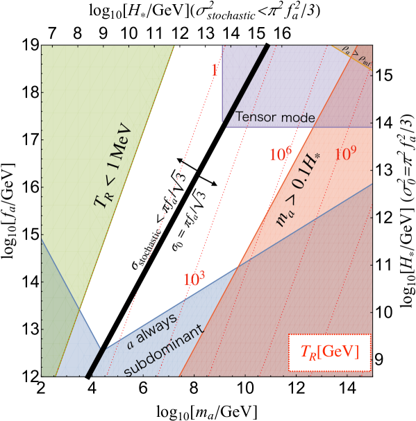
Figure 1: The parameter region in $m_{a}-f_{a}$ plane with the contours of the reheating temperature, $T_{R}$, caused by the ALP decay. On the upper (right) axis, we show $H_{*}$ corresponding to the region left (right) to the black solid line. The left green region is excluded due to the too low reheating temperature which is incompatible with the BBN. The blue region in the bottom does not have a period of the curvaton dominated Universe. In the upper-right purple (orange) region, the tensor mode is too large (the axion-energy dominates over the inflation energy density). In the right red region, $m_{a}>H_{*}$ and the axion-curvaton oscillation starts during inflation. In this figure $c_{\gamma}=1$ is taken.

The viable parameter region in $m_{a}-f_{a}$ plane is shown in Fig.1, with the contour of the reheating temperature. From the right top colored regions are excluded due to the non-observation of the tensor mode, $|n_{s}-1|\gtrsim 0.01$ due to $m_{a}>0.1H_{*}$, subdominant axion until its decay, and the BBN bound in the clockwise direction. In the small orange region in the top-right corner, the ALP energy density during inflation $\rho_{a}\equiv\Lambda^{4}$, is larger than the inflationary energy density $\rho_{\rm inf}\equiv 3H_{*}^{2}M_{\rm pl}^{2}$. Much left (right) to the black solid line has $\Lambda\gg H_{*}$ ($\Lambda\ll H_{*}$) where the corresponding $H_{*}$ is shown in the upper (right) axis. The viable parameter region is in the range

$$100{\rm\,GeV}<m_{a}<10^{12}{\rm\,GeV},10^{12}{\rm\,GeV}<f_{a}\lesssim M_{\rm pl}.$$ (29)

The corresponding inflationary Hubble parameter is

$$10^{8}{\rm\,GeV}<H_{*}<4.7\times 10^{13}{\rm\,GeV}.$$ (30)

The reheating temperature due to the curvaton decay is in the range

$$1{\rm\,MeV}\lesssim T_{R}\lesssim 10^{7}{\rm\,GeV}.$$ (31)

Therefore various baryogenesis scenarios and dark matter productions are comparable. Much before the decay of the axion, the inflaton or the plasma produced from the inflaton may dominate the Universe. In particular, around the blue bottom region, such component is non-negligible even at the reheating by the axion decay. Nevertheless, the baryogenesis or dark matter production should happen relevant to the curvaton $\sigma$ but not the inflaton, because otherwise the baryon or dark matter has “isocurvature”.

In most of the parameter range, we have $n_{s}\approx 1$, which is quite a natural prediction in this scenario. On the other hand, around the boundary of the right red region denoting $m_{a}>0.1H_{*}$, $|n_{s}-1|\sim 0.01$ can be realized. In this case, whether $n_{s}$ is greater or smaller than $1$ is determined by the sign of the curvature $V^{\prime\prime}$ of the potential, which is approximately a 50/50 chance.

Cosmology in axiverse with $n_{s}\approx 1$.– So far, we have shown that the ALP-curvaton scenario is consistent with those solutions to the Hubble tension that predict $n_{s}\approx 1$. The resulting decay constant is consistent with the one for the conventional string axion $f_{a}\sim 10^{15-17}\,$GeV.

This may imply that the Universe is in the axiverse [54, 55, 56, 57, 58, 59, 60, 61, 62, 63], in which there are many axions with masses spread over a wide mass range. In particular, an ALP coupled to the SM gauge bosons is predicted in an M-theory compactification [58]. In this scenario, it is natural that a string axion happens to have the mass in the viable range of Fig.1 and plays the role of the curvaton. In this case, the predicting Universe naturally has $n_{s}\approx 1$.

We comment on a possible relevant cosmology in the axiverse with the stochastic axion curvaton. Lighter axions, if exist, also have the stochastic nature [45, 46]. In the usual single cosine potential with a potential hight $\sim\Lambda_{\rm DM}^{4}$ satisfying $\Lambda_{\rm DM}\gg H_{*}$ a lighter axion tends to dominate the Universe. For the viable inflation scales in Fig.1, the natural mass scale of the axion to explain the dark matter abundance is too heavy to be a stable ALP (see Ref. [53]). In most of the sub-MeV mass range where the ALP is stable and can evade observational constraints, we need to tune the initial amplitude of the ALP in the equilibrium distribution. A special mass range without tuning is $\sim 10^{-18}{\rm\,eV}$ for a decay constant $\sim 10^{16}{\rm\,GeV}$. In this case, the equilibrium distribution is flat and the initial misalignment amplitude is around the decay constant.

With multiple cosine terms which make up a flat-bottomed potential, on the other hand, the axion dark matter can be even lighter without over-closing the Universe [64, 47]. In this case, $H_{*}\lesssim 10^{13}{\rm\,GeV}$ is further needed to evade the isocurvature bound [47].

If a very light axion, whose mass is such light that its energy contribution to the Universe is subdominant, may start its oscillation around or after the recombination. If the light axion gets this kind of potential, the Hubble tension can be relaxed via the early dark energy which is transferred into the axion oscillation energy which scales as radiation [15, 16]. The initial condition of the axion can be set by the stochastic behavior during inflation. In this case, there can also be a domain wall formation depending on whether the initially averaged axion is close to the potential top [65, 25]. The domain wall problem can be evaded since the axion is light.

In addition, the inflation itself may be caused by an axion in the axiverse [66, 67, 68, 69, 70, 71, 72, 73, 74]. In particular, with a flat axion potential top composed by several-cosine terms, the inflation can happen with a sub-Planckian decay constant [68, 70, 72, 73]. The flat top, as well as the flat bottom, can be realized in extra-dimensional models [72, 73, 74]. It is intriguing that such inflaton potential resembles that used for the early dark energy, both of which may be realized in the axiverse or the axion landscape.

QCD axion as curvaton.– A natural question is whether the QCD axion [75, 76, 77, 78] can be the curvaton for our purpose. Naively the answer seems to be negative because of the smallness of the QCD scale. Here we discuss the possibility that the QCD axion acquires an aligned instanton contribution from UV dynamics to the IR QCD instanton. In this case, the QCD axion can be much heavier than the conventional one, while the strong CP problem is solved. To be specific, we consider a mirror SM sector related to the SM by $Z_{2}$ symmetry following [79] (see also the original proposal in Ref.[80]). We assume that the $Z_{2}$ symmetry is broken by a VEV of hidden Higgs, $v_{H}$. $v_{H}$ is much larger than the electroweak (EW) scale.

We consider the (string) axion couplings to gluons and hidden gluons (shown with primes) as follows,

$$-{\cal L}=\frac{\alpha_{s}}{8\pi}(\frac{\sigma}{f_{a}}-\theta_{CP})G\tilde{G}+\frac{\alpha^{\prime}_{s}}{8\pi}(\frac{\sigma}{f_{\alpha}}-\theta_{CP})G^{\prime}\tilde{G}^{\prime}.$$ (32)

at a renormalization scale, $\mu_{\rm RG}(<v_{H})$. At this scale, both sectors are still perturbative. While $\alpha_{s}^{\prime}\sim\alpha_{s}$ at $\mu_{\rm RG}\sim v_{H}$, we have $\alpha_{s}^{\prime}>\alpha_{s}$ at $\mu_{\rm RG}\ll v_{H}$ due to the decoupling of the heavy colored particles in the hidden sector. The hierarchy between $\alpha_{s}^{\prime}$ and $\alpha_{s}$ can be even larger with extra colored particles in both sectors. Those particles get masses around $v_{H}$ in the hidden sector while their $Z_{2}$ partners in the SM sector remain relatively light but not too light to be consistent with the experimental bounds.

Then, non-perturbative effects of the hidden QCD provides a large contribution to the axion potential whose minimum is aligned to the vanishing strong CP phase,

$$V\sim-\Lambda^{\prime 4}\cos{(\frac{\sigma}{f_{a}}-\theta_{CP})},$$ (33)

Note that in the hidden sector the axion gets mass from a pure Yang-Mills instanton due to the decoupling of the hidden quarks. In this case, the axion may not have sizable couplings to the hidden photon unlike the standard QCD axion which mixes with mesons. The dominant decay of the axion is to the SM gluons and it reheats the Universe. This scenario gives a similar parameter region as in Fig.1.

Other possibilities of explaining $n_{s}$ different from $n_{s}^{\rm\Lambda CDM}$ .– When $n_{s}$ is close to, but not very close to 1, the chaotic inflation with a monomial potential $V_{\rm inf}\propto\phi^{p}$ with small $p$ is a simple way to realize such $n_{s}$ together with a suppressed tensor mode [39] (see also [81]). For a sufficiently small $p(>0)$, the predicted spectral index asymptotes to $n_{s}\simeq 0.98$ for the e-folding number $N=50$. However, we need a super-Planckian field excursion, which may be disfavored from the quantum gravity. The multi-natural inflation [68, 70, 72, 73], ALP inflation [82, 83, 84, 85], or the QCD axion inflation [79] also have the parameter region of $n_{s}\sim 1$ (see also Ref.[32] for the mechanism to modify $n_{s}$). The same models can explain $n_{s}<n_{s}^{\rm\Lambda CDM}$.

References

- [1] Planck collaboration, N. Aghanim et al., Planck 2018 results. VI. Cosmological parameters, Astron. Astrophys. 641 (2020) A6 [1807.06209].
- [2] A. G. Riess, L. Macri, S. Casertano, H. Lampeitl, H. C. Ferguson, A. V. Filippenko et al., A 3% Solution: Determination of the Hubble Constant with the Hubble Space Telescope and Wide Field Camera 3, Astrophys. J. 730 (2011) 119 [1103.2976].
- [3] V. Bonvin et al., H0LiCOW – V. New COSMOGRAIL time delays of HE 04351223: to 3.8 per cent precision from strong lensing in a flat CDM model, Mon. Not. Roy. Astron. Soc. 465 (2017) 4914 [1607.01790].
- [4] A. G. Riess et al., A 2.4% Determination of the Local Value of the Hubble Constant, Astrophys. J. 826 (2016) 56 [1604.01424].
- [5] A. G. Riess et al., Milky Way Cepheid Standards for Measuring Cosmic Distances and Application to Gaia DR2: Implications for the Hubble Constant, Astrophys. J. 861 (2018) 126 [1804.10655].
- [6] S. Birrer et al., H0LiCOW - IX. Cosmographic analysis of the doubly imaged quasar SDSS 1206+4332 and a new measurement of the Hubble constant, Mon. Not. Roy. Astron. Soc. 484 (2019) 4726 [1809.01274].
- [7] W. L. Freedman, Cosmology at a Crossroads, Nature Astron. 1 (2017) 0121 [1706.02739].
- [8] L. Verde, T. Treu and A. G. Riess, Tensions between the Early and the Late Universe, Nature Astron. 3 (2019) 891 [1907.10625].
- [9] E. Di Valentino et al., Snowmass2021 - Letter of interest cosmology intertwined II: The hubble constant tension, Astropart. Phys. 131 (2021) 102605 [2008.11284].
- [10] N. Schöneberg, G. Franco Abellán, A. Pérez Sánchez, S. J. Witte, V. Poulin and J. Lesgourgues, The Olympics: A fair ranking of proposed models, 2107.10291.
- [11] A. G. Riess et al., A Comprehensive Measurement of the Local Value of the Hubble Constant with 1 km/s/Mpc Uncertainty from the Hubble Space Telescope and the SH0ES Team, 2112.04510.
- [12] E. Di Valentino, A. Melchiorri, Y. Fantaye and A. Heavens, Bayesian evidence against the Harrison-Zel’dovich spectrum in tensions with cosmological data sets, Phys. Rev. D 98 (2018) 063508 [1808.09201].
- [13] G. Ye, B. Hu and Y.-S. Piao, Implication of the Hubble tension for the primordial Universe in light of recent cosmological data, Phys. Rev. D 104 (2021) 063510 [2103.09729].
- [14] T. Karwal and M. Kamionkowski, Dark energy at early times, the Hubble parameter, and the string axiverse, Phys. Rev. D 94 (2016) 103523 [1608.01309].
- [15] V. Poulin, T. L. Smith, T. Karwal and M. Kamionkowski, Early Dark Energy Can Resolve The Hubble Tension, Phys. Rev. Lett. 122 (2019) 221301 [1811.04083].
- [16] V. Poulin, T. L. Smith, D. Grin, T. Karwal and M. Kamionkowski, Cosmological implications of ultralight axionlike fields, Phys. Rev. D 98 (2018) 083525 [1806.10608].
- [17] M.-X. Lin, G. Benevento, W. Hu and M. Raveri, Acoustic Dark Energy: Potential Conversion of the Hubble Tension, Phys. Rev. D 100 (2019) 063542 [1905.12618].
- [18] F. Niedermann and M. S. Sloth, New early dark energy, Phys. Rev. D 103 (2021) L041303 [1910.10739].
- [19] F. Niedermann and M. S. Sloth, Resolving the Hubble tension with new early dark energy, Phys. Rev. D 102 (2020) 063527 [2006.06686].
- [20] R. Murgia, G. F. Abellán and V. Poulin, Early dark energy resolution to the Hubble tension in light of weak lensing surveys and lensing anomalies, Phys. Rev. D 103 (2021) 063502 [2009.10733].
- [21] T. L. Smith, V. Poulin, J. L. Bernal, K. K. Boddy, M. Kamionkowski and R. Murgia, Early dark energy is not excluded by current large-scale structure data, Phys. Rev. D 103 (2021) 123542 [2009.10740].
- [22] S. Vagnozzi, Consistency tests of CDM from the early integrated Sachs-Wolfe effect: Implications for early-time new physics and the Hubble tension, Phys. Rev. D 104 (2021) 063524 [2105.10425].
- [23] Y. Minami and E. Komatsu, New Extraction of the Cosmic Birefringence from the Planck 2018 Polarization Data, Phys. Rev. Lett. 125 (2020) 221301 [2011.11254].
- [24] T. Fujita, Y. Minami, K. Murai and H. Nakatsuka, Probing axionlike particles via cosmic microwave background polarization, Phys. Rev. D 103 (2021) 063508 [2008.02473].
- [25] F. Takahashi and W. Yin, Kilobyte Cosmic Birefringence from ALP Domain Walls, JCAP 04 (2021) 007 [2012.11576].
- [26] L. M. Capparelli, R. R. Caldwell and A. Melchiorri, Cosmic birefringence test of the Hubble tension, Phys. Rev. D 101 (2020) 123529 [1909.04621].
- [27] M. Reig, The Stochastic Axiverse, JHEP 09 (2021) 207 [2104.09923].
- [28] M. Escudero and S. J. Witte, A CMB search for the neutrino mass mechanism and its relation to the Hubble tension, Eur. Phys. J. C 80 (2020) 294 [1909.04044].
- [29] F.-Y. Cyr-Racine and K. Sigurdson, Limits on Neutrino-Neutrino Scattering in the Early Universe, Phys. Rev. D 90 (2014) 123533 [1306.1536].
- [30] L. Lancaster, F.-Y. Cyr-Racine, L. Knox and Z. Pan, A tale of two modes: Neutrino free-streaming in the early universe, JCAP 07 (2017) 033 [1704.06657].
- [31] C. D. Kreisch, F.-Y. Cyr-Racine and O. Doré, Neutrino puzzle: Anomalies, interactions, and cosmological tensions, Phys. Rev. D 101 (2020) 123505 [1902.00534].
- [32] F. Takahashi, New inflation in supergravity after Planck and LHC, Phys. Lett. B 727 (2013) 21 [1308.4212].
- [33] A. D. Linde and V. F. Mukhanov, Nongaussian isocurvature perturbations from inflation, Phys. Rev. D 56 (1997) R535 [astro-ph/9610219].
- [34] K. Enqvist and M. S. Sloth, Adiabatic CMB perturbations in pre - big bang string cosmology, Nucl. Phys. B 626 (2002) 395 [hep-ph/0109214].
- [35] D. H. Lyth and D. Wands, Generating the curvature perturbation without an inflaton, Phys. Lett. B 524 (2002) 5 [hep-ph/0110002].
- [36] T. Moroi and T. Takahashi, Effects of cosmological moduli fields on cosmic microwave background, Phys. Lett. B 522 (2001) 215 [hep-ph/0110096].
- [37] M. Kawasaki, T. Kobayashi and F. Takahashi, Non-Gaussianity from Curvatons Revisited, Phys. Rev. D 84 (2011) 123506 [1107.6011].
- [38] Planck collaboration, N. Aghanim et al., Planck 2018 results. VI. Cosmological parameters, Astron. Astrophys. 641 (2020) A6 [1807.06209].
- [39] BICEP, Keck collaboration, P. A. R. Ade et al., Improved Constraints on Primordial Gravitational Waves using Planck, WMAP, and BICEP/Keck Observations through the 2018 Observing Season, Phys. Rev. Lett. 127 (2021) 151301 [2110.00483].
- [40] M. Kawasaki, T. Kobayashi and F. Takahashi, Non-Gaussianity from Axionic Curvaton, JCAP 03 (2013) 016 [1210.6595].
- [41] K. Dimopoulos, D. H. Lyth, A. Notari and A. Riotto, The Curvaton as a pseudoNambu-Goldstone boson, JHEP 07 (2003) 053 [hep-ph/0304050].
- [42] A. A. Starobinsky, STOCHASTIC DE SITTER (INFLATIONARY) STAGE IN THE EARLY UNIVERSE, Lect. Notes Phys. 246 (1986) 107.
- [43] A. A. Starobinsky and J. Yokoyama, Equilibrium state of a selfinteracting scalar field in the De Sitter background, Phys. Rev. D 50 (1994) 6357 [astro-ph/9407016].
- [44] R. J. Hardwick, V. Vennin, C. T. Byrnes, J. Torrado and D. Wands, The stochastic spectator, JCAP 10 (2017) 018 [1701.06473].
- [45] P. W. Graham and A. Scherlis, Stochastic axion scenario, Phys. Rev. D 98 (2018) 035017 [1805.07362].
- [46] F. Takahashi, W. Yin and A. H. Guth, QCD axion window and low-scale inflation, Phys. Rev. D 98 (2018) 015042 [1805.08763].
- [47] S. Nakagawa, F. Takahashi and W. Yin, Stochastic Axion Dark Matter in Axion Landscape, JCAP 05 (2020) 004 [2002.12195].
- [48] T. Moroi, K. Mukaida, K. Nakayama and M. Takimoto, Axion Models with High Scale Inflation, JHEP 11 (2014) 151 [1407.7465].
- [49] M. Kawasaki, K. Kohri and N. Sugiyama, Cosmological constraints on late time entropy production, Phys. Rev. Lett. 82 (1999) 4168 [astro-ph/9811437].
- [50] M. Kawasaki, K. Kohri and N. Sugiyama, MeV scale reheating temperature and thermalization of neutrino background, Phys. Rev. D 62 (2000) 023506 [astro-ph/0002127].
- [51] K. Ichikawa, M. Kawasaki and F. Takahashi, The Oscillation effects on thermalization of the neutrinos in the Universe with low reheating temperature, Phys. Rev. D 72 (2005) 043522 [astro-ph/0505395].
- [52] Planck collaboration, Y. Akrami et al., Planck 2018 results. IX. Constraints on primordial non-Gaussianity, Astron. Astrophys. 641 (2020) A9 [1905.05697].
- [53] S.-Y. Ho, F. Takahashi and W. Yin, Relaxing the Cosmological Moduli Problem by Low-scale Inflation, JHEP 04 (2019) 149 [1901.01240].
- [54] E. Witten, Some Properties of O(32) Superstrings, Phys. Lett. B 149 (1984) 351.
- [55] P. Svrcek and E. Witten, Axions In String Theory, JHEP 06 (2006) 051 [hep-th/0605206].
- [56] J. P. Conlon, The QCD axion and moduli stabilisation, JHEP 05 (2006) 078 [hep-th/0602233].
- [57] A. Arvanitaki, S. Dimopoulos, S. Dubovsky, N. Kaloper and J. March-Russell, String Axiverse, Phys. Rev. D 81 (2010) 123530 [0905.4720].
- [58] B. S. Acharya, K. Bobkov and P. Kumar, An M Theory Solution to the Strong CP Problem and Constraints on the Axiverse, JHEP 11 (2010) 105 [1004.5138].
- [59] T. Higaki and T. Kobayashi, Note on moduli stabilization, supersymmetry breaking and axiverse, Phys. Rev. D 84 (2011) 045021 [1106.1293].
- [60] M. Cicoli, M. Goodsell and A. Ringwald, The type IIB string axiverse and its low-energy phenomenology, JHEP 10 (2012) 146 [1206.0819].
- [61] M. Demirtas, C. Long, L. McAllister and M. Stillman, The Kreuzer-Skarke Axiverse, JHEP 04 (2020) 138 [1808.01282].
- [62] V. M. Mehta, M. Demirtas, C. Long, D. J. E. Marsh, L. Mcallister and M. J. Stott, Superradiance Exclusions in the Landscape of Type IIB String Theory, 2011.08693.
- [63] V. M. Mehta, M. Demirtas, C. Long, D. J. E. Marsh, L. McAllister and M. J. Stott, Superradiance in string theory, JCAP 07 (2021) 033 [2103.06812].
- [64] R. Daido, T. Kobayashi and F. Takahashi, Dark Matter in Axion Landscape, Phys. Lett. B 765 (2017) 293 [1608.04092].
- [65] M. Y. Khlopov, S. G. Rubin and A. S. Sakharov, Primordial structure of massive black hole clusters, Astropart. Phys. 23 (2005) 265 [astro-ph/0401532].
- [66] K. Freese, J. A. Frieman and A. V. Olinto, Natural inflation with pseudo - Nambu-Goldstone bosons, Phys. Rev. Lett. 65 (1990) 3233.
- [67] F. C. Adams, J. R. Bond, K. Freese, J. A. Frieman and A. V. Olinto, Natural inflation: Particle physics models, power law spectra for large scale structure, and constraints from COBE, Phys. Rev. D 47 (1993) 426 [hep-ph/9207245].
- [68] M. Czerny and F. Takahashi, Multi-Natural Inflation, Phys. Lett. B 733 (2014) 241 [1401.5212].
- [69] M. Czerny, T. Higaki and F. Takahashi, Multi-Natural Inflation in Supergravity, JHEP 05 (2014) 144 [1403.0410].
- [70] M. Czerny, T. Higaki and F. Takahashi, Multi-Natural Inflation in Supergravity and BICEP2, Phys. Lett. B 734 (2014) 167 [1403.5883].
- [71] T. Higaki, T. Kobayashi, O. Seto and Y. Yamaguchi, Axion monodromy inflation with multi-natural modulations, JCAP 10 (2014) 025 [1405.0775].
- [72] D. Croon and V. Sanz, Saving Natural Inflation, JCAP 02 (2015) 008 [1411.7809].
- [73] T. Higaki and F. Takahashi, Elliptic inflation: interpolating from natural inflation to R2-inflation, JHEP 03 (2015) 129 [1501.02354].
- [74] T. Higaki and Y. Tatsuta, Inflation from periodic extra dimensions, JCAP 07 (2017) 011 [1611.00808].
- [75] R. D. Peccei and H. R. Quinn, CP Conservation in the Presence of Instantons, Phys. Rev. Lett. 38 (1977) 1440.
- [76] R. D. Peccei and H. R. Quinn, Constraints Imposed by CP Conservation in the Presence of Instantons, Phys. Rev. D 16 (1977) 1791.
- [77] S. Weinberg, A New Light Boson?, Phys. Rev. Lett. 40 (1978) 223.
- [78] F. Wilczek, Problem of Strong and Invariance in the Presence of Instantons, Phys. Rev. Lett. 40 (1978) 279.
- [79] F. Takahashi and W. Yin, Challenges for heavy QCD axion inflation, JCAP 10 (2021) 057 [2105.10493].
- [80] H. Fukuda, K. Harigaya, M. Ibe and T. T. Yanagida, Model of visible QCD axion, Phys. Rev. D 92 (2015) 015021 [1504.06084].
- [81] Planck collaboration, Y. Akrami et al., Planck 2018 results. X. Constraints on inflation, Astron. Astrophys. 641 (2020) A10 [1807.06211].
- [82] R. Daido, F. Takahashi and W. Yin, The ALP miracle: unified inflaton and dark matter, JCAP 05 (2017) 044 [1702.03284].
- [83] R. Daido, F. Takahashi and W. Yin, The ALP miracle revisited, JHEP 02 (2018) 104 [1710.11107].
- [84] F. Takahashi and W. Yin, ALP inflation and Big Bang on Earth, JHEP 07 (2019) 095 [1903.00462].
- [85] F. Takahashi and W. Yin, QCD axion on hilltop by a phase shift of , JHEP 10 (2019) 120 [1908.06071].