Topological Signal Processing over Cell Complexes

Abstract

The Topological Signal Processing (TSP) framework has been recently developed to analyze signals defined over simplicial complexes, i.e. topological spaces represented by finite sets of elements that are closed under inclusion of subsets [1]. However, the same inclusion property represents sometimes a too rigid assumption that prevents the application of simplicial complexes to many cases of interest. The goal of this paper is to extend TSP to the analysis of signals defined over cell complexes, which represent a generalization of simplicial complexes, as they are not restricted to satisfy the inclusion property. In particular, the richer topological structure of cell complexes enables them to reveal cycles of any order, as representative of data features. We propose an efficient method to infer the topology of cell complexes from data by showing how their use enables sparser edge signal representations than simplicial-based methods. Furthermore, we show how to design optimal finite impulse response (FIR) filters operating on solenoidal and irrotational signals in order to minimize the approximation error with respect to the desired spectral masks.

I Introduction

In the last years, the ever growing interest in machine learning and complex networks has motivated the development of models and tools to represent and analyze data on topological spaces. The recent field of Graph Signal Processing (GSP) [2] has emerged as a powerful tool for the analysis of signals defined over the vertices of a graph, which is a simple topological space where edges encode pairwise relationships among data. However, in many applications, for example in gene regulatory networks, the multiway relationships among complex molecules, like genes, proteins or metabolites, cannot be grasped using only pairwise relationships [3]. To overcome the limitations of graph-based approaches, a more general topological signal processing framework (TSP), operating over higher-order structures able to capture multiway relations such as simplicial complexes, has been recently introduced in [1], [4], [5]. Simply put, a topological space is a set $\mathcal{V}$ of elements along with a set of multiway relations among them. An abstract simplicial complex is an example of topological space represented by a set $\mathcal{S}$ composed of subsets of various order satisfying the inclusion property, so that if a set $\mathcal{B}$ belongs to $\mathcal{S}$ then any subset of $\mathcal{B}$ also belongs to $\mathcal{S}$ [6]. Recently, the authors of [5] provide a comprehensive tutorial on the broad topic of signal processing over hypergraphs and simplicial complexes, whereas [7] focuses on the design of finite impulse response filters to process signals defined over simplicial complexes. However, in many cases of interest, the inclusion constraint associated with simplicial complexes may be quite limiting. For example, in biological networks, the presence of a reaction among a group of molecules, e.g. genes or proteins, does not imply that a reaction occurs also among any subgroup of elements. A more general structure, not constrained to respect the inclusion property, but still retaining the algebraic richness of simplicial complexes, is given by cell complexes [8], [9]. Cell complexes are defined as a collection of cells that are sets of points whose subsets does not necessarily belong to the complex. Cell complexes have already been applied to model complex systems [10], to solve ranking problems [11], to perform neural network-type computation over rich topological spaces [12] or for hierarchical message passing schemes [13]. The processing of signals over cell complexes has been recently introduced in [14] where it is shown how to design filters to be used in neural networks defined over cell complexes.

Our goal in this paper is to extend the TSP framework of [1] to signals defined over cell complexes, proposing an algorithm to infer the structure of the complex from data and a method to find sparse edge signal representations that enable, using sampling theory, the reconstruction of the whole set of edge signals from the observation of a subset of samples. Furthermore, we propose a method to design optimal FIR filters for the solenoidal and irrotational components. Finally, we corroborate the effectiveness of the proposed methods with numerical tests, by showing how the use of cell complexes yields a substantial performance gain with respect to simplicial-based methods.

II Introduction to Cell Complexes

In this section we introduce the notion of cell complex (CC) and then we present its algebraic representation. Given a discrete set $\mathcal{V}$ of $N$ vertices $v_{i}$, $i=1,\ldots,N$, a collection $\Delta$ of non-empty finite subsets of $\mathcal{V}$ is called an abstract simplicial complex if it satisfies the inclusion property, meaning that, for every set $X$ in $\Delta$, and every non-empty subset $Y\subseteq X$, the set $Y$also belongs to $\Delta$. An element of the complex is called a $k$-simplex (or simplex of order $k$) and it simply denotes a set of $k+1$ elements (vertices). If embedded into a real domain, a simplicial complex is composed of vertices ($0$-simplices), edges ($1$-simplices), triangles ($2$-simplices), and so on.
A more general structure, not constrained to respect the inclusion property, but still retaining the algebraic richness of simplicial complexes, is given by the cell complexes [8], [9]. An abstract cell complex (ACC) [15], [16], denoted as $\mathcal{C}=\{\mathcal{S},\prec_{b},\text{dim}\}$, is a set $\mathcal{S}$ of elements along with a binary relation $\prec_{b}$, called the bounding relation, and with a dimension function, denoted by $\text{dim}(x)$, that assigns to each $x\in\mathcal{S}$ a non-negative integer, satisfying the following two properties:

1. if $x\prec_{b}y$ and $y\prec_{b}z$, then $x\prec_{b}z$ follows (transitivity);

2. if $x\prec_{b}y$, then $\text{dim}(x)<\text{dim}(y)$ (monotonicity).

An $n$-cell, denoted by $c^{n}$, is a cell $c$ with dimension $n$; $0$-cells are named vertices. Given two cells $x,y\in\mathcal{S}$, if $x\prec_{b}y$, we say that $x$ bounds $y$ and $x$ is called a proper side of $y$. The boundary $\partial x^{n}$ of an $n$-dimensional cell $x^{n}$ is defined as the set of all cells of dimension less than $n$ that bound $x^{n}$. An ACC is $k$-dimensional if the dimensions of all its cells are less than or equal to $k$. The closed cell including its boundary is denoted by $\bar{x}^{n}=x^{n}\cup\partial x^{n}$. Two cells $x,y$ are incident if $x\prec_{b}y$ or $y\prec_{b}x$. More specifically, we say that $x$ is lower incident to $y$ if $x\prec_{b}y$ and upper incident to $y$ if $y\prec_{b}x$. To associate a topological structure to an ACC, we need to introduce first the concept of open and closed subsets. A subset $U$ of $\mathcal{C}=\{\mathcal{S},\prec_{b},\text{dim}\}$ is called open (closed) in $\mathcal{C}$ iff, for every element $x$ of $U$, all elements $y$ of $\mathcal{C}$ upper (lower) bounding $x$ are also in $U$ [15]. According to the axioms of topology, any intersection of a finite number of open (closed) subsets is open (closed).
An ACC can be embedded into a Euclidean space. In such a case, $0$-cells represent vertices, $1$-cells are edges and $2$-cells are polygons. Then, simplicial complexes are particular cases of cell complexes where $2$-cells are triangles. However, cell complexes do not need to respect the inclusion property of simplicial complexes, so that a polygon with more than three sides cannot be a simplex but it can be a cell.
Similarly to simplicial complexes, the structure of a $K$-complex is fully described by the set of its incidence (boundary) matrices $\mbox{$\mathbf{B}$}_{k}$, $k=1,\ldots,K$, where the $k$-th matrix encodes which $k$-cell is incident to which $(k-1)$-cell. As with graphs, we need to introduce the orientation of a cell complex by generalizing the concept of orientation of a simplex [9]. Defining the transposition as the permutation of two elements, two orientations are equivalent if each of them can be recovered from the other through an even number of transpositions. To define the orientation of a $k$-cell, we may apply a simplicial decomposition [9], which consists in subdividing the cell into a set of internal $k$-simplices, so that, by orienting a single internal simplex, the orientation propagates to the entire cell. An oriented $k$-cell may then be represented as $c^{k}=[c^{k-1}_{1},\ldots,c^{k-1}_{M}]$ where two consecutive $(k-1)$-cells, $c^{k-1}_{i}$ and $c^{k-1}_{i+1}$ shares a common $(k-2)$-cell boundary. Then, given an orientation of the cells, two $k$-order cells are lower adjacent if they share a common face of order $k-1$ or upper adjacent if both are faces of a cell of order $k+1$. Given an oriented cell complex ${\cal C}$, the set of its incidences matrices $\mbox{$\mathbf{B}$}_{k}$ with $k=1,\ldots,K$ is defined as follows:

$$B_{k}(i,j)=\left\{\begin{array}[]{rll}0,&\text{if}\;c^{k-1}_{i}\not\prec_{b}c^{k}_{j}\\ 1,&\text{if}\;c^{k-1}_{i}\prec_{b}c^{k}_{j}\;\text{and}\;c^{k-1}_{i}\sim c^{k}_{j}\\ -1,&\text{if}\;c^{k-1}_{i}\prec_{b}c^{k}_{j}\;\text{and}\;c^{k-1}_{i}\nsim c^{k}_{j}\\ \end{array}\right.$$ (1)

where we use the notation $c^{k-1}_{i}\sim c^{k}_{j}$ to indicate that the orientations of $c^{k-1}_{i}$ and $c^{k}_{j}$ are coherent and $c^{k-1}_{i}\not\sim c^{k}_{j}$ to indicate opposite orientations.

Let us consider a cell complex of order two $\mathcal{C}=\{\mathcal{V},\mathcal{E},\mathcal{P}\}$ where $\mathcal{V}$, $\mathcal{E}$, $\mathcal{P}$ denote the set of $0$, $1$ and $2$-cells, i.e. vertices, edges and polygons, respectively. We denote their cardinality by $|\mathcal{V}|=V$, $|\mathcal{E}|=E$ and $|\mathcal{P}|=P$. Then, the two incidence matrices describing the connectivity of the complex are $\mbox{$\mathbf{B}$}_{1}\in\mathbb{R}^{V\times E}$ and $\mbox{$\mathbf{B}$}_{2}\in\mathbb{R}^{E\times P}$, where $\mbox{$\mathbf{B}$}_{2}$ can be written as

$$\mbox{$\mathbf{B}$}_{2}=[\mbox{$\mathbf{B}$}_{T},\mbox{$\mathbf{B}$}_{Q},\ldots,\mbox{$\mathbf{B}$}_{P_{S}}]$$ (2)

where $\mbox{$\mathbf{B}$}_{T}$, $\mbox{$\mathbf{B}$}_{Q}$ and $\mbox{$\mathbf{B}$}_{P_{S}}$ indicate the incidences between edges and, respectively, triangles, quadrilaterals, up to polygons with $P_{S}$ sides, where each polygon does not include any internal chord between any pair of its vertices. An interesting property of the incidence matrices is that $\mbox{$\mathbf{B}$}_{k}\mbox{$\mathbf{B}$}_{k+1}=\mathbf{0},\;\forall k$. To describe the structure of a $K$-cell complex, we can use the higher order combinatorial Laplacian matrices given by [17]:

$$\begin{split}&\mbox{$\mathbf{L}$}_{0}=\mbox{$\mathbf{B}$}_{1}\mbox{$\mathbf{B}$}_{1}^{T},\\ &\mbox{$\mathbf{L}$}_{k}=\mbox{$\mathbf{B}$}_{k}^{T}\mbox{$\mathbf{B}$}_{k}+\mbox{$\mathbf{B}$}_{k+1}\mbox{$\mathbf{B}$}_{k+1}^{T}\;\;\mbox{for}\;k=1,\ldots,K-1\\ &\mbox{$\mathbf{L}$}_{K}=\mbox{$\mathbf{B}$}_{K}^{T}\mbox{$\mathbf{B}$}_{K}\end{split}$$ (3)

where $\mbox{$\mathbf{L}$}_{k}^{l}:=\mbox{$\mathbf{B}$}_{k}^{T}\mbox{$\mathbf{B}$}_{k}$ and $\mbox{$\mathbf{L}$}_{k}^{u}:=\mbox{$\mathbf{B}$}_{k+1}\mbox{$\mathbf{B}$}_{k+1}^{T}$ are the lower and upper Laplacians, expressing, respectively, the lower and upper adjacencies of the $k$-order cells. Considering w.l.o.g. the first order Laplacian, i.e.

$$\mbox{$\mathbf{L}$}_{1}=\mbox{$\mathbf{L}$}_{1}^{l}+\mbox{$\mathbf{L}$}_{1}^{u}=\mbox{$\mathbf{B}$}_{1}^{T}\mbox{$\mathbf{B}$}_{1}+\mbox{$\mathbf{B}$}_{2}\mbox{$\mathbf{B}$}_{2}^{T},$$ (4)

it holds: i) the eigenvectors associated with the nonzero eigenvalues of $\mbox{$\mathbf{L}$}_{1}^{l}=\mathbf{B}^{T}_{1}\mathbf{B}_{1}$ are orthogonal to the eigenvectors associated with the nonzero eigenvalues of $\mbox{$\mathbf{L}$}_{1}^{u}=\mathbf{B}_{2}\mathbf{B}_{2}^{T}$ and viceversa; ii) the eigenvectors associated with the nonzero eigenvalues $\lambda^{1}$ of $\mathbf{L}_{1}$ are either the eigenvectors of $\mbox{$\mathbf{L}$}_{1}^{l}$ or those of $\mbox{$\mathbf{L}$}_{1}^{u}$; and, finally, iii) the nonzero eigenvalues of $\mathbf{L}_{1}$ are either the eigenvalues of $\mbox{$\mathbf{L}$}_{1}^{l}$ or those of $\mbox{$\mathbf{L}$}_{1}^{u}$. This spectral structure of $\mbox{$\mathbf{L}$}_{1}$ induces and interesting decomposition of the whole space $\mathbb{R}^{E}$, the so-called Hodge decomposition [18], given by

$$\mathbb{R}^{E}\triangleq\text{img}(\mbox{$\mathbf{B}$}_{1}^{T})\oplus\text{ker}(\mbox{$\mathbf{L}$}_{1})\oplus\text{img}(\mbox{$\mathbf{B}$}_{2})$$ (5)

where the vectors in $\text{ker}(\mbox{$\mathbf{L}$}_{1})$ are also in $\text{ker}(\mbox{$\mathbf{B}$}_{1})$ and $\text{ker}(\mbox{$\mathbf{B}$}_{2}^{T})$.

III Analysis of signals defined over CCs

In this section we extend the fundamental tools to analyze signals defined over simplicial complexes provided in [1] to cell complexes. We focus w.l.o.g. on cell complexes of order $2$. Given a cell complex $\mathcal{C}=\{\mathcal{V},\mathcal{E},\mathcal{P}\}$, the signals on vertices, edges and polygons are defined by the following maps: $\mbox{\boldmath$s$}^{0}:{\cal V}\rightarrow\mathbb{R}^{V}$, $\mbox{\boldmath$s$}^{1}:{\cal E}\rightarrow\mathbb{R}^{E}$, and $\mbox{\boldmath$s$}^{2}:{\cal P}\rightarrow\mathbb{R}^{P}$. A useful orthogonal basis to represent signals of various order, capturing the connectivity properties of the complex, is given by the eigenvectors of the corresponding higher order Laplacian. Then, generalizing graph spectral theory, we can introduce a notion of Cell complex Fourier Transform (CFT) for signals defined over cell complexes. Let us consider the eigendecomposition $\mbox{$\mathbf{L}$}_{k}=\mbox{$\mathbf{U}$}_{k}\boldsymbol{\Lambda}_{k}\mbox{$\mathbf{U}$}_{k}^{T}$ where $\mbox{$\mathbf{U}$}_{k}$ is the eigenvectors matrix and $\boldsymbol{\Lambda}_{k}$ is a diagonal matrix with entries the eigenvalues $\lambda_{i}^{k}$ of $\mbox{$\mathbf{L}$}_{k}$, with $i=1,\ldots,E$. Then, we define the $k$-order CFT as the projection of a $k$-order signal onto the eigenvectors of $\mbox{$\mathbf{L}$}_{k}$, i.e.

$$\hat{\mbox{\boldmath$s$}}^{k}\triangleq\mbox{$\mathbf{U}$}_{k}^{T}\mbox{\boldmath$s$}^{k}.$$ (6)

A signal $\mbox{\boldmath$s$}^{k}$ can then be represented in terms of its CFT coefficients as $\mbox{\boldmath$s$}^{k}=\mbox{$\mathbf{U}$}_{k}\hat{\mbox{\boldmath$s$}}^{k}.$ Exploiting the Hodge decomposition in (5), we may always express a signal $\mbox{\boldmath$s$}^{1}$ as the sum of three orthogonal components [18], i.e.

$$\mbox{\boldmath$s$}^{1}=\mbox{$\mathbf{B}$}_{1}^{T}\mbox{\boldmath$s$}^{0}+\mbox{$\mathbf{B}$}_{2}\mbox{\boldmath$s$}^{2}+\mbox{\boldmath$s$}^{1}_{H}.$$ (7)

In analogy to vector calculus terminology, the first component $\mbox{\boldmath$s$}^{1}_{irr}:=\mbox{$\mathbf{B}$}_{1}^{T}\mbox{\boldmath$s$}^{0}$ is called the irrotational component since, using the equality $\mbox{$\mathbf{B}$}_{1}\mbox{$\mathbf{B}$}_{2}=\mathbf{0}$, it has zero curl, i.e. $\mbox{$\mathbf{B}$}_{2}^{T}\mbox{\boldmath$s$}^{1}_{irr}=\mathbf{0}$, while the second term $\mbox{\boldmath$s$}^{1}_{sol}:=\mbox{$\mathbf{B}$}_{2}\mbox{\boldmath$s$}^{2}$ is the solenoidal component, since its divergence defined as $\mbox{$\mathbf{B}$}_{1}\mbox{\boldmath$s$}^{1}_{sol}$ is zero. Finally, the component $\mbox{\boldmath$s$}^{1}_{H}$ is the harmonic component since it belongs to $\text{ker}(\mbox{$\mathbf{L}$}_{1})$ and it has zero curl and zero divergence.

IV Inference of cell complexes topology

Hinging on the algorithm proposed in [1], in this section we present a method to infer the topology of a cell complex from data. Our goal is to show that cell complexes enable more sparse signal representations, for a given signal reconstruction error, than simplicial complexes. We start with inference of the topology of cell complexes of order $2$ from the observations of a set of $M$ edge signals $\mbox{$\mathbf{Y}$}^{1}=[\mbox{\boldmath$y$}^{1}(1),\ldots,\mbox{\boldmath$y$}^{1}(M)]$. We assume that the graph topology, i.e. the 0-order Laplacian matrix $\mbox{$\mathbf{L}$}_{0}=\mbox{$\mathbf{B}$}_{1}\mbox{$\mathbf{B}$}_{1}^{T}$, is known. Then, since $\mbox{$\mathbf{L}$}_{1}=\mbox{$\mathbf{B}$}_{1}^{T}\mbox{$\mathbf{B}$}_{1}+\mbox{$\mathbf{B}$}_{2}\mbox{$\mathbf{B}$}_{2}^{T}$, we only need to infer the incidence matrix $\mbox{$\mathbf{B}$}_{2}$. More specifically, we infer the presence of $2$-cells, i.e. polygons of any order, by selecting the columns $\mbox{\boldmath$b$}_{n}$ of the boundary matrix $\mbox{$\mathbf{B}$}_{2}$ for which the total circulation of the observed edge signals along the corresponding $2$-cell is minimum. As a first step, we need to check if the upper Laplacian $\mbox{$\mathbf{L}$}_{1}^{u}$ is really needed to represent the observed data. Then, since the solenoidal and harmonic signals are the only components depending on $\mbox{$\mathbf{B}$}_{2}$, we first project the observed signals onto the space orthogonal to the irrotational component. Thereby, defining the matrix $\mbox{$\mathbf{U}$}_{irr}$ containing as columns the eigenvectors of $\mbox{$\mathbf{L}$}_{1}^{l}$ associated with the non-zero eigenvalues, we compute

$$\mbox{\boldmath$y$}^{1}_{sH}(i)=(\mbox{$\mathbf{I}$}-\mbox{$\mathbf{U}$}_{irr}\mbox{$\mathbf{U}$}_{irr}^{T})\mbox{\boldmath$y$}^{1}(i),\;i=1,\ldots,M.$$ (8)

Denoting with $\mbox{$\mathbf{Y}$}^{1}_{sH}=[\mbox{\boldmath$y$}^{1}_{sH}(1),\ldots,\mbox{\boldmath$y$}^{1}_{sH}(M)]$ the resulting matrix, we measure the energy of $\mbox{$\mathbf{Y}$}^{1}_{sH}$ by taking its norm: If the norm falls below a threshold, we set $\mbox{$\mathbf{B}$}_{2}=\mathbf{0}$, otherwise we proceed with the inference of $\mbox{$\mathbf{B}$}_{2}$. To do that, we extend the algorithm proposed in [1], minimizing the total variation of the observed data along all polygons. Indicating with $q_{n}$ a binary coefficient equal to $1$ (or $0$) if the corresponding cell is present (or not), we have

$$\mbox{$\mathbf{B}$}_{2}\mbox{$\mathbf{B}$}_{2}^{T}=\sum_{n=1}^{N_{c}}q_{n}\mbox{\boldmath$b$}_{n}\mbox{\boldmath$b$}_{n}^{T},$$ (9)

where $N_{c}$ denotes the number of possible $2$-cells in the complex. Our goal is to find the entries of the vector $\mbox{\boldmath$q$}=[q_{1},\ldots,q_{N_{c}}]$ as the solution of the following problem:

$$\begin{array}[]{lll}\underset{\mbox{\boldmath$q$}\in\{0,1\}^{N_{c}}}{\min}&\displaystyle\sum_{n=1}^{N_{c}}q_{n}\mbox{tr}(\mbox{$\mathbf{Y}$}^{1\,T}_{sH}\mbox{\boldmath$b$}_{n}\mbox{\boldmath$b$}_{n}^{T}\mbox{$\mathbf{Y}$}^{1}_{sH})\\ \quad\text{s.t.}&\parallel\mbox{\boldmath$q$}\parallel_{0}=q^{\star}\end{array}$$ (10)

where the number of components $q^{\star}$ is found in a validation phase. Interestingly, this problem, albeit non-convex, admits a closed form solution. Defining the nonnegative coefficients $d_{n}=\sum_{i=1}^{M}\mbox{\boldmath$y$}_{sH}^{1\;T}(i)\mbox{\boldmath$b$}_{n}\mbox{\boldmath$b$}_{n}^{T}\mbox{\boldmath$y$}_{sH}^{1}(i)$, the optimal solution can be derived by sorting in increasing order the coefficients $d_{n}$ and selecting the columns of $\mbox{$\mathbf{B}$}_{2}$ corresponding to the indices of the $q^{\star}$ lower coefficients $d_{n}$.

V Sparse signal representation

Once we have $\mbox{$\mathbf{L}$}_{1}$, we can find a basis of the observed edge flows using the eigenvectors of $\mbox{$\mathbf{L}$}_{1}$. Our goal is to find the optimal trade-off between the sparsity of the signal representation and the data fitting error by solving the following basis pursuit problem:

$$\begin{array}[]{lll}\underset{{\mbox{\boldmath$s$}}^{1}\in\mathbb{R}^{E}}{\text{min}}&\parallel{\mbox{\boldmath$s$}}^{1}\parallel_{1}\\ \;\;\text{s.t.}&\parallel{\mbox{\boldmath$y$}}^{1}-\mbox{$\mathbf{V}$}{\mbox{\boldmath$s$}}^{1}\parallel_{F}\leq\epsilon\end{array}$$ (11)

where $\mbox{$\mathbf{V}$}=\mbox{$\mathbf{U}$}_{1}$ is the eigenvectors matrix associated with $\mbox{$\mathbf{L}$}_{1}$. Exploiting the bandlimited property enforced by the sparse representations, we reconstruct the overall set of edge signals from a subset of edge samples using a generalization of the MaxDet greedy sampling strategy in [19] and the recovering rule (49) in [1].

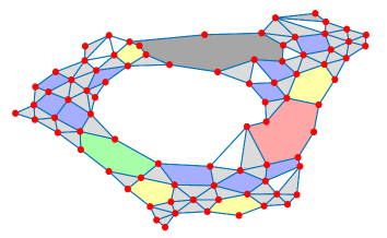
(a)

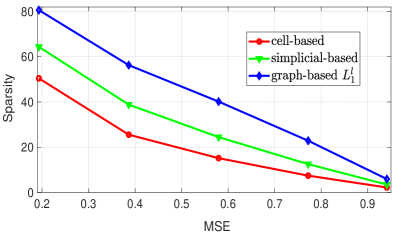
(b)

Figure 1: (a) Inferred cell complex; (b) Sparsity vs. mean squared error.

To test the effectiveness of the proposed methods, in Fig. $1(a)$ we represent an example of inferred $2$-cell complex from the observation of $M=100$ independent realizations of edges signals over a complex with $N=82$ nodes, $E=165$ edges and $75$ polygons. Then, we also infer, from the same data-set, a simplicial complex. To compare the different topological spaces, in Fig. $1(b)$ we report the signal sparsity (number of nonzero entries of ${\mbox{\boldmath$s$}}^{1}$) versus the mean squared error (MSE) obtained by solving problem in (11), using for $\mathbf{V}$ the eigenvector matrix associated to $\mbox{$\mathbf{L}$}_{1}^{l}$ and to the first order Laplacians of the inferred simplicial and cell complexes. We can notice from Fig. $1(b)$ that, using a cell-based approach, we can achieve a better sparsity/MSE trade-off compared to simplicial based methods, where only triangles are taken into account, or to graph-based methods, where the signal basis is given by the eigenvectors of $\mbox{$\mathbf{L}$}_{1}^{l}$. Then, exploiting the bandlimited property of the signals enforced by their sparse representations, we can use the sampling theory to reconstruct the overall edge signal vector from a subset of edge values, generalizing the approach of [19] to cell complexes. In Fig. $2$ we illustrate an example of reconstruction, in the presence of noise with variance $\sigma_{n}^{2}=0.01$, plotting the MSE in the signal reconstruction versus the number of samples used to retrieve the overall signal. From Fig. $2$, we can assess the substantial performance improvement of the cell-based method with respect to graph- and simplicial-based approaches.

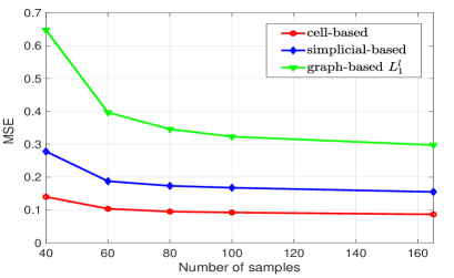
Figure 2: Mean squared error versus number of samples.

VI FIR filters over cell complexes

In this section we propose a method to design FIR filters for the solenoidal and irrotational signals observed over the edges of cell complexes. Graph filters have been largely investigated in the field of GSP [20], [21] and their extension to signals defined over the edges of simplicial complex have been considered in [7]. Recently, filters defined over cell complexes have been proposed in [14]. We focus on the design of FIR filters for the solenoidal and irrotational signals, since the filtering of the harmonic component needs an independent design as we deeply investigate in [22].
As a straight generalization of graph filters, a FIR filter based on the first order Laplacian is a local operator assuming the following form

$$\mbox{$\mathbf{H}$}=\sum_{k=0}^{K}a_{k}\mbox{$\mathbf{L}$}^{k}_{1}$$ (12)

where $\{a_{k}\}_{k=0}^{K}$ are the filter coefficients, $K$ is the filter length and $\mbox{$\mathbf{L}$}^{0}_{1}=\mbox{$\mathbf{I}$}$. Note that the matrices $\mbox{$\mathbf{L}$}^{k}_{1}$, $k=1,\ldots,K$ contain information about the neighbors of order $K$, then they represent local operators which linearly combine edge signals from upper and lower neighboring cells. Because of the condition $\mbox{$\mathbf{B}$}_{1}\mbox{$\mathbf{B}$}_{2}=\mathbf{0}$, it holds $\mbox{$\mathbf{L}$}_{1}^{k}=(\mbox{$\mathbf{L}$}_{1}^{l})^{k}+(\mbox{$\mathbf{L}$}_{1}^{u})^{k}$. Thus the filtering operation in (12) reduces to the following two orthogonal filters

$$\mbox{\boldmath$x$}^{1}=\sum_{k=0}^{K}a_{k}^{I}(\mbox{$\mathbf{L}$}_{1}^{l})^{k}\mbox{\boldmath$s$}^{1}+\sum_{k=0}^{K}a_{k}^{s}(\mbox{$\mathbf{L}$}_{1}^{u})^{k}\mbox{\boldmath$s$}^{1}$$ (13)

which suggests an independent design of the filters coefficients $a_{k}^{I}$, $a_{k}^{s}$ for, respectively, the irrotational and solenoidal components, as also proposed in [7]. Using the CFT defined in (6), the spectrum of the filter output becomes

$$\begin{split}\hat{\mbox{\boldmath$x$}}^{1}&=\mbox{$\mathbf{U}$}_{1}^{T}\mbox{\boldmath$x$}^{1}=\left(\sum_{k=0}^{K}a_{k}^{I}\boldsymbol{\Lambda}_{l}^{k}+\sum_{k=0}^{K}a_{k}^{s}\boldsymbol{\Lambda}_{u}^{k}\right)\hat{\mbox{\boldmath$s$}}^{1}\end{split}$$ (14)

where we used (13) by splitting the diagonal matrix $\boldsymbol{\Lambda}_{1}$ containing the eigenvalues of $\mbox{$\mathbf{L}$}_{1}$ into two diagonal matrices $\boldsymbol{\Lambda}_{l}$ and $\boldsymbol{\Lambda}_{u}\in\mathbb{R}^{E\times E}$ containing the eigenvalues of the lower and upper Laplacians, respectively. It is worth to notice that, by definition of spectral filtering, if the Laplacian $\mbox{$\mathbf{L}$}_{1}$ contains eigenvalues of multiplicity greater than $1$, the filter is not able to distinguish the components belonging to the subspace associated to the multiple eigenvalue. A typical example occurs when the embedding of the abstract cell complex onto a real domain yields a structure with a number of holes $N_{h}>1$. In such a case, $\mbox{$\mathbf{L}$}_{1}$ has a null eigenvalue of dimension $N_{h}$ [6]. If we rewrite (14) by distinguishing the term with $k=0$, as

$$\hat{\mbox{\boldmath$x$}}^{1}=\left(a_{0}\mbox{$\mathbf{I}$}+\sum_{k=1}^{K}a_{k}^{I}\boldsymbol{\Lambda}_{l}^{k}+\sum_{k=1}^{K}a_{k}^{s}\boldsymbol{\Lambda}_{u}^{k}\right)\hat{\mbox{\boldmath$s$}}^{1}$$ (15)

it is evident that all vectors belonging to the kernel of $\mbox{$\mathbf{L}$}_{1}$ are simply scaled by a common coefficient $a_{0}$. Note that a coefficient $a_{0}\neq 0$ in (15) has an adverse effect on the disjoint filtering of the irrotational and solenoidal signals since it lets all the signal components pass through the filter. In this paper, for lack of space, we focus on the filtering of the solenoidal and irrotational signals by designing two independent FIR filters in which the constant term is removed, so that they assume the form

$$\mbox{\boldmath$x$}^{1}=\left(\sum_{k=1}^{K_{l}}a_{k}^{I}(\mbox{$\mathbf{L}$}^{l}_{1})^{k}+\sum_{k=1}^{K_{u}}a_{k}^{s}(\mbox{$\mathbf{L}$}^{u}_{1})^{k}\right)\mbox{\boldmath$s$}^{1}$$ (16)

where each filter of length, respectively, $K_{l}$ and $K_{u}$ imposes a spectral mask on the desired component while filtering out all the others. Let us assume that the operators we wish to implement through FIR filters are given by

$$\begin{split}\mathbf{H}_{irr}=\mbox{$\mathbf{U}$}_{irr}h^{I}(\boldsymbol{\Lambda}_{irr})\mbox{$\mathbf{U}$}_{irr},\qquad\mathbf{H}_{sol}=\mbox{$\mathbf{U}$}_{sol}h^{s}(\boldsymbol{\Lambda}_{sol})\mbox{$\mathbf{U}$}_{sol}^{T},\end{split}$$ (17)

where $\mbox{$\mathbf{U}$}_{irr}$ and $\mbox{$\mathbf{U}$}_{sol}$ are the matrices containing the eigenvectors associated with the non-zero eigenvalues of $\mbox{$\mathbf{L}$}_{1}^{l}$ and $\mbox{$\mathbf{L}$}_{1}^{u}$, respectively, and $\boldsymbol{\Lambda}_{irr}$, $\boldsymbol{\Lambda}_{sol}$ are the diagonal matrices with entries the corresponding non-zero eigenvalues. The diagonal entries $h^{I}(\lambda_{i})$ and $h^{s}(\lambda_{i})$ of the matrices $h^{I}(\boldsymbol{\Lambda}_{irr})$ and $h^{s}(\boldsymbol{\Lambda}_{sol})$ are the frequency responses of the filters associated with the irrotational and solenoidal eigenvalues. Our goal is to approximate the operators in (17) with the following FIR filters

$$\hat{\mbox{$\mathbf{H}$}}_{irr}=\displaystyle\sum_{k=1}^{K_{l}}a_{k}^{I}(\mbox{$\mathbf{L}$}_{1}^{l})^{k},\quad\hat{\mbox{$\mathbf{H}$}}_{sol}=\displaystyle\sum_{k=1}^{K_{u}}a_{k}^{s}(\mbox{$\mathbf{L}$}_{1}^{u})^{k}.$$ (18)

The filters coefficients $\mbox{\boldmath$a$}^{I}=(a_{k}^{I})_{k=1}^{K_{l}}$ and $\mbox{\boldmath$a$}^{s}=(a_{k}^{s})_{k=1}^{K_{u}}$ can be found solving the following least-squares problems in the spectral domain

$$\underset{\mathbf{a}^{I}\in\mathbb{R}^{K}}{\min}\quad\parallel\mathbf{h}^{I}-\boldsymbol{\Phi}_{I}\mbox{\boldmath$a$}^{I}\parallel^{2}_{F}\quad\text{and}\quad\underset{\mathbf{a}^{s}\in\mathbb{R}^{K}}{\min}\quad\parallel\mathbf{h}^{s}-\boldsymbol{\Phi}_{s}\mbox{\boldmath$a$}^{s}\parallel^{2}_{F}$$ (19)

where $\mathbf{h}^{I}:=\text{diag}(h^{I}(\boldsymbol{\Lambda}_{irr})),\mathbf{h}^{s}:=\text{diag}(h^{s}(\boldsymbol{\Lambda}_{sol}))$ and

$$\boldsymbol{\Phi}_{I}:=[\boldsymbol{\lambda}_{I},\boldsymbol{\lambda}_{I}^{2},\ldots,\boldsymbol{\lambda}_{I}^{K_{l}}],\;\boldsymbol{\Phi}_{s}:=[\boldsymbol{\lambda}_{s},\boldsymbol{\lambda}_{s}^{2},\ldots,\boldsymbol{\lambda}_{s}^{K_{u}}],$$ (20)

with $\boldsymbol{\lambda}_{I}$ and $\boldsymbol{\lambda}_{s}$ the column vectors with entries, respectively, the non-zero eigenvalues of the lower and upper Laplacians. The optimal solutions of the two least-squares problems in (19) are given in closed form by

$$\mbox{\boldmath$a$}^{I}=\boldsymbol{\Phi}_{I}^{{\dagger}}\mathbf{h}^{I},\qquad\mbox{\boldmath$a$}^{s}=\boldsymbol{\Phi}_{s}^{{\dagger}}\mathbf{h}^{s}$$ (21)

where $\boldsymbol{\Phi}^{{\dagger}}$ denotes the Moore-Penrose pseudo-inverse of $\boldsymbol{\Phi}$. Note that, defining $\mathbf{h}=[\mathbf{h}^{s};\mathbf{h}^{I}]$ and $\boldsymbol{\Phi}_{t}=[\boldsymbol{\Phi}_{s};\boldsymbol{\Phi}_{I}]$, a single filter can be derived by solving the following least-squares problem

$$\underset{\mbox{\boldmath$a$}\in\mathbb{R}^{K}}{\min}\quad\parallel\mbox{\boldmath$h$}-\boldsymbol{\Phi}_{t}{\mbox{\boldmath$a$}}\parallel^{2}_{F}$$ (22)

whose optimal solution is given in closed form by $\mbox{\boldmath$a$}=\boldsymbol{\Phi}^{{\dagger}}_{t}\mbox{\boldmath$h$}.$

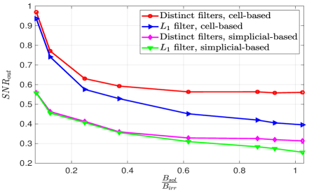
Figure 3: SNR at the filter output for the solenoidal part vs. $B_{sol}/B_{irr}$.

In Fig. $3$ to evaluate the goodness of the proposed filtering strategy we report the signal-to-noise ratio (SNR) observed at the output of the solenoidal filter versus the ratio between the solenoidal and irrotational signal bandwidths. We consider the optimal FIR filters for the solenoidal and irrotational filters obtained by solving the problems in (19) or by using a single $\mbox{$\mathbf{L}$}_{1}$-based FIR filter as solution of the problem in (22). It can be observed from Fig. $3$ that the independent design of the two filters coefficients provides a performance gains with respect to a single $\mbox{$\mathbf{L}$}_{1}$-based filter and to simplicial-based methods.

VII Conclusions

In this paper we extended topological signal processing from simplicial complexes to richer topological spaces as cell complexes. We show as TSP over cell complex enables sparser signal representations than simplicial complexes based approaches. Furthermore, we focused on the optimal design of FIR filters for the solenoidal and irrotational signals to minimize the approximation error with respect to the desired spectral masks.

References

- [1] S. Barbarossa and S. Sardellitti, “Topological signal processing over simplicial complexes,” IEEE Trans. Signal Process., vol. 68, pp. 2992–3007, Mar. 2020.
- [2] A. Ortega, P. Frossard, J. Kovačević, J. M. F. Moura, and P. Vandergheynst, “Graph signal processing: Overview, challenges, and applications,” Proc. of the IEEE, vol. 106, no. 5, pp. 808–828, May 2018.
- [3] R. Lambiotte, M. Rosvall, and I. Scholtes, “From networks to optimal higher-order models of complex systems,” Nature Physics, vol. 15, no. 4, pp. 313–320, 2019.
- [4] S. Barbarossa and S. Sardellitti, “Topological signal processing: Making sense of data building on multiway relations,” IEEE Signal Process. Mag., vol. 37, no. 6, pp. 174–183, Nov. 2020.
- [5] M. T. Schaub, Y. Zhu, J.-B. Seby, T. M. Roddenberry, and S. Segarra, “Signal processing on higher-order networks: Livin’ on the edge… and beyond,” Signal Processing, p. 108149, 2021.
- [6] J. R. Munkres, Elements of algebraic topology, CRC press, 2018.
- [7] M. Yang, E. Isufi, M. T. Schaub, and G. Leus, “Finite impulse response filters for simplicial complexes,” arXiv preprint arxiv.org/abs/2103.12587, Mar. 2021.
- [8] A. Hatcher, Algebraic topology, Cambr. Univ. Press, 2005.
- [9] L. J. Grady and J. R. Polimeni, Discrete calculus: Applied analysis on graphs for computational science, Sprin. Sci. & Busin. Media, 2010.
- [10] D. Mulder and G. Bianconi, “Network geometry and complexity,” Journal of Statistical Physics, vol. 173, no. 3, pp. 783–805, 2018.
- [11] A. N. Hirani, K. Kalyanaraman, and S. Watts, “Least squares ranking on graphs, Hodge Laplacians, time optimality, and iterative methods,” arXiv preprint arXiv:1011.1716, 2010.
- [12] M. Hajij, K. Istvan, and G. Zamzmi, “Cell complex neural networks,” NeurIPS 2020, Workshop Topol. Data Anal. and Beyond, 2020.
- [13] C. Bodnar, F. Frasca, N. Otter, Y.-G. Wang, P. Liò, G. Montúfar, and M. Bronstein, “Weisfeiler and Lehman go cellular: CW networks,” Advanc. Neur. Infor. Process. Syst., vol. 34, 2021.
- [14] T. M. Roddenberry, M. T. Schaub, and M. Hajij, “Signal processing on cell complexes,” arXiv preprint arXiv:2110.05614, 2021.
- [15] R. Klette, “Cell complexes through time,” in Vision Geometry IX. Int. Soc. for Opt. and Photon., 2000, vol. 4117, pp. 134–145.
- [16] E. Steinitz, “Beiträge zur analysis situs,” Sitz-Ber. Berlin Math. Ges, vol. 7, pp. 29–49, 1908.
- [17] T. E. Goldberg, “Combinatorial Laplacians of simplicial complexes,” Senior Thesis, Bard College, 2002.
- [18] L.-H. Lim, “Hodge Laplacians on graphs,” S. Mukherjee (Ed.), Geometry and Topology in Statistical Inference, Proc. Sympos. Appl. Math., 76, AMS, 2015.
- [19] M. Tsitsvero, S. Barbarossa, and P. Di Lorenzo, “Signals on graphs: Uncertainty principle and sampling,” IEEE Trans. Signal Process., vol. 64, no. 18, pp. 4845–4860, Sept. 2016.
- [20] A. Sandryhaila and J. M. F. Moura, “Discrete signal processing on graphs: Frequency analysis,” IEEE Trans. Signal Process., vol. 62, no. 12, pp. 3042–3054, June 2014.
- [21] S. Segarra, A. G. Marques, and A. Ribeiro, “Optimal graph-filter design and applications to distributed linear network operators,” IEEE Trans. Signal Process., vol. 65, no. 15, pp. 4117–4131, Aug. 2017.
- [22] S. Sardellitti and S. Barbarossa, “Signal representation and filtering over cell complexes,” to be submitted on IEEE Trans. Signal Process., 2021.