Real-Time Estimation of COVID-19 Infections: Deconvolution and Sensor Fusion

Abstract

We propose, implement, and evaluate a method to estimate the daily number of new symptomatic COVID-19 infections, at the level of individual U.S. counties, by deconvolving daily reported COVID-19 case counts using an estimated symptom-onset-to-case-report delay distribution. Importantly, we focus on estimating infections in real-time (rather than retrospectively), which poses numerous challenges. To address these, we develop new methodology for both the distribution estimation and deconvolution steps, and we employ a sensor fusion layer (which fuses together predictions from models that are trained to track infections based on auxiliary surveillance streams) in order to improve accuracy and stability.

, , and

1 Introduction

Accurate, real-time estimates of incident infections play a critical role in informing the public health response to the spread of a disease through a population. However, official metrics on disease activity published by traditional public health surveillance systems in the United States do not in fact reflect activity in real-time, as they suffer from some degree of latency due to the way their reporting pipelines are set up and implemented.

With addressing the latency in traditional public health reporting a part of the motivation, the last decade has seen a rise in the development of digital surveillance streams in public health. Search and social media trends have constituted much of the focus (e.g., Brownstein, Freifeld and Madoff, 2009; Ginsberg et al., 2009; Salathé et al., 2012; Kass-Hout and Alhinnawi, 2013; Paul and Dredze, 2017). More broadly, auxiliary surveillance streams that operate outside of traditional public health surveillance, like online surveys, medical device logs, or electronic medical records, have also received significant attention (e.g., Kass-Hout and Zhang, 2011; Carlson et al., 2013; Viboud et al., 2014; Smolinski et al., 2015; Santillana et al., 2016; Charu et al., 2017; Yang et al., 2019; Ackley et al., 2020; Leuba et al., 2020; Radin et al., 2020).

Auxiliary surveillance can improve not only on the timeliness but also on the accuracy and robustness of traditional public health reporting. Auxiliary data streams have therefore become an integral part of modern systems for disease nowcasting (e.g., McIver and Brownstein, 2014; Santillana et al., 2015; Yang, Santillana and Kou, 2015; Farrow, 2016; Jahja et al., 2019; Brooks, 2020), which, put broadly, are used to estimate the contemporaneous value of a signal that will only be fully observed at a later date, using partial or noisy data.

1.1 Surveillance During the Pandemic

During the COVID-19 pandemic, public health surveillance has produced, on one hand, some of the most detailed public health data that the U.S. has ever seen, such as daily, county-level data on reported COVID-19 cases and deaths. It has also, on the other hand, painted an imperfect picture of situational awareness, which created a number of downstream challenges for the public health response. See, e.g., Rosenfeld and Tibshirani (2021) and references therein for an overview of the issues. In this paper, we identify a few issues surrounding COVID-19 case reporting in particular, propose methodology to address them, and implement and evaluate this proposal over eight months of pandemic data.

To give some background, in the early days of the pandemic, a handful of non-gonvermental groups such as JHU CSSE (Dong, Du and Gardner, 2020) (and also the COVID Tracking Project, the New York Times, and USAFacts) became known as the most trustworthy sources for aggregate public health reporting data on COVID-19 in the U.S. They were founded around the idea of scraping COVID-19 data published daily on dashboards that are run by local public health authorities (such as state and county departments of public health), which, at the time, provided more accurate and timely data than federal health authorities (probably due to unrecoverable failures at one or more points along the reporting pipeline). In fact, not only in the early days of the pandemic, but throughout, the data published by these groups has been invaluable for decision-makers, modelers, journalists, and the general public; for example, data from JHU CSSE remains the gold standard for COVID-19 case and death forecast evaluation in the COVID-19 Forecast Hub (Reich Lab, 2020), a community-driven repository of forecasts that serves as the official source for forecasting communications by the U.S. CDC.

Turning our focus now to case reporting, JHU scrapes cumulative case numbers that are published daily on local health authority dashboards, and subsequently derives a notion of case incidence based on day-to-day differences in cumulative counts. Note that, by construction, this definition of incidence reflects the number of new COVID-19 cases that are reported (to the public) on any given day. Of course, this is not the same as the number of new cases by date tested, specimen collection date, or symptom onset date. Any of the latter options would be more informative (increasingly so) as a definition of incidence; revamping our surveillance systems so that they can directly provide these and other aggregates of interest to the public health response is a critical task for future public health crises.

The reality of the current pandemic: alignment by report date is the only option available, given the data published broadly on local health authority dashboards, hence collected and aggregated by data scrapers. JHU publishes the number of new COVID-19 case reports per U.S. county, daily, at a 1-day lag. However, since report dates can lag behind symptom onset dates by many days (a typical lag is around 5-10, but lags can be up to 30 days or more; see Figure 3), this is actually giving us a glimpse into COVID activity in the recent past, rather than the present.

Importantly, the CDC publishes a de-identified patient-level data set (“line list”) on COVID-19 infections (Centers for Disease Control and Prevention, COVID-19 Response, 2020a), which provides a symptom onset date column. In principle, this should allow us to construct a notion of case incidence that is aligned by symptom onset date, but this is not possible in practice, due to two barriers. First, the CDC only publishes updates to the line list monthly (due to the complexity of managing this data set). Second, and more problematically, this line list is fraught with missingness, extending well beyond missingness in the symptom onset column: the total number of COVID-19 cases according to this line list (whether the symptom onset date is observed or not) is far less than the total number of cases from JHU (e.g., in early September 2021, the CDC line list reports about 30 million total versus about 40 million from JHU), and some states (such as Texas) appear to missing nearly all of their cases in the line list altogether (see Figure 2).

1.2 Nowcasting by Deconvolution

In what follows in this paper, we use the CDC line list to estimate a delay distribution between symptom onset and report dates, and then use this delay distribution to deconvolve daily numbers of new case reports published by JHU CSSE to estimate daily numbers of new symptomatic infections. Moreover, we train models that track historical trends between past infection estimates and auxiliary signals of COVID-19 activity from Delphi’s COVIDcast project (Reinhart et al., 2021), and we fuse together predictions from these models in order to improve the accuracy and robustness of our estimates of new infections for the most recent 10 days (where deconvolution is particularly challenging). An illustration is given in Figure 1.

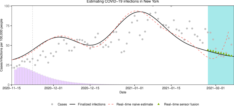
Figure 1: Illustration of estimating latent infections from reported cases. The dashed red line displays infection rates estimated “naively” in real-time, by directly deconvolving case data up through early February 2021, while the solid black line display infection rates estimated using finalized data from roughly four months afterwards. The blue region on the right-hand side highlights a period in which the real-time estimate deviates substantially from the finalized one, due to the fact that we are lacking sufficient (future) case observations needed to perform a “full” deconvolution. The green triangles represent real-time nowcasts made by sensor fusion, which reduces the volatility of the real-time estimate and tracks the finalized estimate nicely. Lastly, the (scaled) reporting delay distribution estimated at the midpoint of November 2020 is drawn in purple, with the median reporting delay (8 days) marked as a dotted gray line.

We focus on estimating new infections in real-time, laying out a framework for an operational nowcasting system that is forced to cope with all of the challenges of disease tracking using provisional data. At any given nowcast date $t$, to estimate the number of symptomatic infections at day $t-k$ (for small values of $k$, such as $k=1,2,\ldots$), we make sure to use data that would have actually been available at $t$. This not only affects the way we carry out all of our experiments (model training and evaluation), it also leads us to develop some new interesting methodology to deal with the issue of right truncation (highlighted in Figure 1 by the blue region). For example, in order to estimate the delay distribution in real-time, we develop a Kaplan-Meier-like procedure to deal with a kind of right censoring that occurs in the line list. We also develop specialized regularization techniques to control the volatility of estimates around the nowcast date in an optimization problem that we solve for real-time deconvolution.

An outline for this paper is as follows. In Section 2, we cover various preliminary details about the problem setup. Retrospective construction of the delay distribution and deconvolution are described in Section 3, whereas real-time estimation is the focus in Section 4. Sensor fusion is covered in Section 5, and extensive evaluations—comparing nowcasts made in real-time to those made retrospectively (using “finalized” data that would have only been available much later), are performed in Section 6. In Section 7, we conclude with a discussion and describe a few directions for future work.

R and Python code for reproducing all figures and results in this paper can be found at https://github.com/cmu-delphi/stat-sci-nowcast.

1.3 Related Work

In the computational epidemiology literature, the term “nowcasting” has been applied to a variety of related but distinct estimation problems. Broadly speaking, what these problems have in common is that they are about real-time estimation of some quantity, based on partial or noisy data. They differ in what is being estimated, and whether this quantity will eventually be fully observed (after enough time has passed) or whether it is latent. Examples in the former non-latent setting, which span applications in influenza, dengue, and COVID-19, include Yang, Santillana and Kou (2015); Farrow (2016); Jahja et al. (2019); Brooks (2020); McGough et al. (2020); Hawryluk et al. (2021).

The latent setting exhibits another degree of diversity within itself. In our work, we target symptomatic COVID-19 infections, which, to be perfectly clear, is a latent time series. Another example along similar lines is Goldstein et al. (2009), who estimate influenza infection incidence via Bayesian deconvolution of mortality data. Meanwhile, other authors might view inferring latent infections as just a stepping stone toward ultimately estimating the instantaneous reproductive number $R_{t}$, a key epidemic parameter. Important contributions to the methodology on real-time estimation of $R_{t}$ include: Bettencourt and Ribeiro (2008), who use a local approximation to the SIR model, and Cori et al. (2013); Thompson et al. (2019), who use a discretization of the renewal equation within a Bayesian framework. For a thorough review and comparison of these methods, see Gostic et al. (2020). The latter paper also discusses in some detail the importance of properly modeling the delay between infection onset and case report, and the issue of right truncation, which, as we will see, are central issues in our paper as well.

The aforementioned methods have been applied and extended to build systems for real-time $R_{t}$ nowcasting during the COVID-19 pandemic by Abbott et al. (2020); Systrom, Vladek and Krieger (2020); Chitwood et al. (2021). A key difference between these approaches and ours is that they infer infections through forward-filling: loosely speaking, they convolve forward a candidate estimate of infections, obtain feedback by comparing the result to measured cases, and iterate to refine estimates. This can be effective given accurate prior knowledge, but of course it can be hard to judge the accuracy of prior knowledge in practice. We take a more flexible approach and estimate infections via direct deconvolution. Our approach is nonparametric, but is still fairly simple and computationally efficient. We also focus on fusing in auxiliary sources of information in order to improve real-time accuracy and robustness. We remark that, if estimates of $R_{t}$ were desired, then these could certainly be inferred as a by-product of our infection nowcasts.

Finally, deconvolution has been extensively studied for many years in many fields, notably signal and image processing, where deconvolution is sometimes called deblurring. As an inverse problem, deconvolution is ill-posed in settings in which the convolution operator is not known exactly or observations are made with noise (Oppenheim and Verghese, 2017). Approaches to overcome this traditionally involve regularization, as in the classical Wiener deconvolution (Wiener, 1964), which stabilizes the inversion using an estimated signal-to-noise ratio. Alternative approaches employ familiar regularization techniques such as $\ell_{1}$ and $\ell_{2}$ penalities (Taylor, Banks and McCoy, 1979; Debeye and Van Riel, 1990). Most related to our paper is deconvolution using total variation regularization, first proposed by Rudin and Osher (1994), and now a central tool in signal and image processing.

2 Preliminaries

In the remainder of this paper, we develop a framework for estimating the daily symptomatic COVID-19 infection rate (where by “rate” we mean a count per 100,000 people, the standard units in epidemiology), concentrating on infections that will eventually result in a reported COVID-19 case. To be clear on nomenclature: for convenience, we will often abbreviate “symptomatic infection” by “infection” (and so, terms like “infection onset” and “infection rate” should be implicitly interpreted as symptomatic). To estimate infection rates, we deconvolve reported case rates with an estimated symptom-onset-to-case-report delay distribution. To reiterate, we use case data from JHU CSSE (Dong, Du and Gardner, 2020), and to infer the delay distribution, we use a de-identified line list on patient-level infections from the CDC (Centers for Disease Control and Prevention, COVID-19 Response, 2020a).

Auxiliary Indicators.

After deconvolution, we improve our infection rate estimates by incorporating a number of contemporaneous signals that track COVID activity—we will also refer to these as indicators—which are publicly available through Delphi’s COVIDcast API (Reinhart et al., 2021). The five indicators that we consider, described below, provide auxiliary information on COVID-19 outside of traditional public heath reporting. Here and throughout, we abbreviate COVID-like illness by CLI.

1. Change Healthcare COVID (CHNG-COVID): The percentage of outpatient visits that have confirmed COVID-19 diagnostic codes, based on de-identified Change Healthcare medical claims data.

2. Change Healthcare CLI (CHNG-CLI): The percentage of outpatient visits that have COVID-like diagnostic codes, based on the same data.

3. Doctor Visits CLI (DV-CLI): The same definition as CHNG-CLI, but applied to de-identified medical claims data from other health systems partners.

4. COVID Trends and Impact Survey CLI in the community (CTIS-CLIIC): The estimated percentage of people reporting illness in their household or local community, based on Delphi’s COVID Trends and Impact Survey (CTIS), in partnership with Facebook.

5. Google searches for anosmia and ageusia (Google-AA): A measure of volume for Google queries related to anosmia or ageusia (loss of smell or taste), from Google’s COVID-19 Search Trends data set.

Roughly speaking, we study these particular indicators (ordered roughly from “late” to “early”) because conceptually they reflect data measurements that would be made at some period of time in between infection onset and case report to a public health authority, and therefore would be relevant in inferring latent infection rates. More information on these indicators and their underlying data sources is given in Reinhart et al. (2021). For more information on CTIS in particular, see Salomon et al. (2021); and for a study of how these and similar indicators can improve COVID-19 forecasting, see McDonald et al. (2021).

Sensor Fusion.

For each of the auxiliary indicators described above, we train a model to estimate latent infection rates from indicator values, using historical data (described in Section 5.1). At each nowcast date, we then use such a model to estimate the latent infection rate from the current indicator value, which gives a total of five estimates (one from each of the five models), along with a sixth estimate coming from an autoregressive model trained on historical estimated infection rates. We will refer these six contemporaneous estimates as sensors.

In this paper, we consider (as described in Section 5.3) various methods for combining these estimates into a single estimate of the infection rate, which we will call sensor fusion methods. Broadly speaking, sensor fusion is a form of ensembling, which is ubiquitous in in predictive modeling in statistics and machine learning, as it can often help improve both accuracy and robustness. In our particular application, the sensors themselves are constructed from data streams operating outside of traditional public health reporting, which itself contributes an additional important angle in terms of robustness.

2.1 Problem Setup

Estimation Period.

For every day $t$ in between October 1, 2020 and June 1, 2021 inclusive (243 days in total), we estimate the symptomatic infection rate at day $t-k$, using only data that would have been as of time $t$, which in this context we call the nowcast date. Estimation of the latent infection rate at time $t-k$ (for positive $k$) is technically a backcast, though we will not be careful to distinguish this notationally from nowcasting, and will generally refer to this as nowcasting at lag $k$. We produce estimates for each $k=1,\ldots,10$, a total of 10 targets per nowcast date $t$.

When we say above that nowcasts are made using data that would have been available as of a given nowcast date $t$, we mean that we adhere not to only the real-time availability (latency) of signals at $t$, but also the version of the data published at $t$—simply put, imagine that we “rewind” the clock to time $t$ and query the API to receive the data that would have been returned then. This is possible becausse the COVIDcast API records and provides access to all historical versions of data, as described in Reinhart et al. (2021). As epidemic data is often subject to revision, if we train and evaluate models on “finalized” data (that would have been available only at a much later time point) then this can lead to inaccurate conclusions about real-time model performance; see, e.g., McDonald et al. (2021).

Further, it is worth noting that reported case data from JHU is available at a 1-day lag, and we assume that there is at least another 1-day lag between symptom onset and case report (explained in Section 3.2). Hence through real-time deconvolution alone we would be able to make nowcasts at a 2-day lag at the earliest. Making nowcasts at a 1-day lag is possible with sensor fusion, using auxiliary signals with 1-day latency (explained in Section 5). In this sense, sensor fusion is able to improve not only accuracy, but also latency, and buys us 1 extra day.

Geographic Scope.

We produce nowcasts at the county resolution, but for computational purposes, we restrict our attention to the 200 U.S. counties with the highest population. We additionally produce estimates for each of the 50 U.S. states. (Some of the methodology that we use for sensor fusion requires a geographical hierarchy, thus using the remaining $\approx$ 3000 U.S. counties we aggregate these within each state to create “rest-of-state” jurisdictions, and make estimates for these as well, for the purposes or maintaining such a hierachy.)

Evaluation.

We evaluate all nowcasts made in between October 1, 2020 and June 1, 2021 inclusive (243 days in total) and at each of the 250 locations in consideration (50 states and the 200 largest counties) against latent infection rate estimates obtained by deconvolving the case rate data available as of August 30, 2021. We will refer to the latter as finalized infection rate estimates (as opposed to real-time ones); details are given in Section 3.3.

2.2 Confounding

Estimates of COVID infections obtained by deconvolving reported cases will generally underestimate the true number of infections, because many infections are undetected or untested, and as such, do not appear later on in case reports. If we wanted to estimate the true number of symptomatic infections from case reports, then we would need to have some sense of the fraction of symptomatic infections that go untested. Of course, this only gets more complicated if we extend our consideration to both symptomatic and asymptomatic infections.

Other authors, e.g., Chitwood et al. (2021), have taken the ambitious step of proposing and implementing frameworks with parameters that account for such confounding. However, adjustments for case ascertainment and asymptomatic infections generally rely, at least to some nontrivial extent, on model assumptions (typically, mechanistic ones) that are difficult to substantiate.

We take a different perspective and pose the problem as one of real-time deconvolution only. We seek to answer the question:

Can we estimate—in real-time—the number of new symptomatic COVID-19 infections that will eventually appear in case reports?

Hence, by construction, confounding is not a problem that we even attempt to reconcile (because the target we track, infections that eventually show up in case reports, simply inherits any confounding that would be present in the case reporting stream in the first place).

Our approach can be seen as one that runs in parallel (rather than in contradiction) to an approach that explicitly models and removes the effects of confounding in case reporting. We focus on addressing the deconvolution problem as carefully as possible, with a concern for real-time estimation, and an eye toward using auxiliary signals to improve accuracy and robustness. Estimates of parameters that account for confounding (that comes from other work focused on these aspects) could certainly be applied to our deconvolution estimates post hoc in order to adjust them appropriately; we revisit this idea in the discussion.

Lastly, under an assumption that the confounding acts as a multiplicative bias that changes slowly over time, our real-time infection rate estimates—themselves subject to confounding, as explained above—can be post-processed to derive real-time approximately unconfounded estimates of $R_{t}$. This is also described in the discussion.

3 Retrospective Deconvolution

In this section, we study and fit a convolutional model between infections and reported cases. We adopt a retrospective angle here and do not concern ourselves with data availability or versioning issues; this is covered in the next section.

3.1 Convolutional Model

For simplicity, we introduce the convolutional model in just a single location. We denote by $y_{t}$ the number of new cases that are reported at time $t$, and by $x_{t}$ the number of new infections that have onset at time $t$. Our jumping-off point is the following model:

$$\mathbb{E}[y_{t}\,|\,x_{s},s\leq t]=\sum_{s=1}^{t}\pi_{t}(s)\,x_{s},$$ (1)

where for each $s\leq t$,

$$\pi_{t}(s)=\mathbb{P}\big{(}\text{case report at $t$}\,|\,\text{infection onset at $s$}\big{)}.$$ (2)

We refer to the probabilities above as delay probabilities at time $t$, and the entire sequence $(\pi_{t}(s):s\leq t)$, as the delay distribution at time $t$.

The justification for (1), (2) is elementary: to count $y_{t}$, we enumerate all infections that ever occurred in the past:

$$y_{t}=\sum_{s=1}^{t}\sum_{i=1}^{x_{s}}1\{\text{the $i^{\mathrm{th}}$ infection at $s$ gets reported at $t$}\}.$$

Taking a conditional expectation on both sides above, and using linearity, delivers (1), (2).

In the next subsections, we will describe how to estimate the probabilities $\pi_{t}(s)$ in (2), and how to use this alongside the observed case reports $y_{t}$ in order to estimate the latent infections in (1).

3.2 Estimating the Delay Distribution

At the outset, we place the following assumptions on the delay distribution in order to make its estimation (using the CDC line list data, to be described shortly) more tractable.

Assumption 1.

Infections are always reported within $d=45$ days; that is, $\pi_{t}(s)=0$ whenever $s<t-d$.

Assumption 2.

The probability of zero delay is zero; that is, $\pi_{t}(t)=0$.

Assumption 3.

The delay distribution is geographically invariant (it is the same for any location).

Assumption 1 is innocuous. The vast majority of pairs of recorded infection dates and report dates in the CDC line list data fall within $d=45$ days of one another. Assumption 2 is perhaps less innocuous but still fairly minor, and it is a consequence of the fact that a delay of zero (infection date equal to report date) has been used inconsistently in the CDC line list: this could mean a true delay of zero, or it could be a code for missingness.

Assumption 3 is the most noteworthy and troublesome. We do not believe it to be true that different locations actually have identical patterns of delay between infections and case reports; conversely, we expect there to be a considerable amount of variability between locations in this regard. While we do allow the delay distribution to change over time (see Figure 3 for evidence for the importance of this), we consider Assumption 3 to be a weakness of our work. However, the data is simply not there in the CDC line list to warrant location-specific estimation of the delay distribution (see Figure 2), thus we resort to estimating a nation-wide delay distribution.

Meanwhile, it is worth pointing out that better (location-specific) estimates of the delay distribution could be simply plugged into our deconvolution methodology (detailed in Section 3.3) to yield better estimates of latent infections. This would carry over to all of the real-time methodology for deconvolution and sensor fusion (in Section 4) as well. In other words, a strength of our methodology is that it can treat the delay distribution as an input, and a user (say, a local health official) can replace the default nation-wide delay distribution with a more-informed local one in order to get more-informed local estimates.

In light of Assumptions 1 and 2, we change our notation henceforth, and rewrite (1), (2) as:

$$\mathbb{E}[y_{t}\,|\,x_{s},s\leq t]=\sum_{k=1}^{d}p_{t}(k)\,x_{t-k},$$ (3)

where for $k=1,\ldots,d$,

$$p_{t}(k)=\mathbb{P}\big{(}\text{case report at $t$}\,|\,\text{onset at $t-k$}\big{)}.$$ (4)

CDC Line List.

The CDC provides de-identified patient-level surveillance data on COVID-19 in both public and restricted forms (Centers for Disease Control and Prevention, COVID-19 Response, 2020a, b). The restricted one is made available under a data use agreement. The public line list contains the same patient-level records as the restricted one, but it has geographic details withheld. (There is another publicly available that contains geographic details, but withholds temporal details). We use the public data set in this paper for estimating the delay distribution, since missingness compels us to make nation-wide (rather than location-specific) estimates.

It is worth noting that the line list is itself provisional and subject to revision. Furthermore, the CDC only publishes updates to the line list monthly. In this paper, for simplicity, we use a single version of the CDC line list—released on September 9, 2021—to construct all delay distributions. Nonetheless, in our real-time nowcasting experiments, we restrict our access to data in this line list that would have been available at each nowcast date $t$ (rows whose report date to the CDC is at most $t$) to construct delay distribution estimates at $t$. This is highly nontrivial, due to bias induced by truncation of data after $t$ (see Section 4.2).

Missing Values.

The CDC line list (both public and restricted data sets) is subject to a high degree of missingness. Such missingness manifests itself in a variety of ways. For the public line list published on September 9, 2021:

• it has 29,851,450 rows, compared to 39,365,080 cumulative cases reported by JHU CSSE on September 9, 2021;

• 8.64% of rows are missing the case report date (the cdc_report_dt column);

• 53.6% of rows are missing the symptom onset date (the onset_dt column);

• of all rows in which symptom onset date is present, the case report date is also present, but when a report date is missing in practice it sometimes gets filled in with the onset date, clouding the interpretation of a zero delay.

Due to the last point, we exclude zero in the construction of all delay distribution estimates, in what follows.

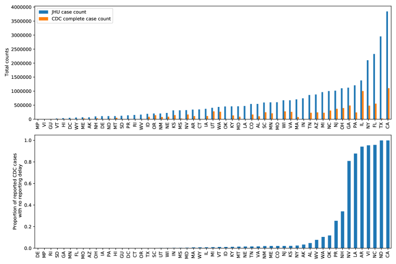
Figure 2: Top: cumulative case count per state on June 1, 2021, as reported by JHU CSSE, compared to the complete case count (where both onset date and report date are observed) per state up through the same date, in the CDC restricted line list. Most states have less than 50% of the cases appear in complete form in the line list, and some (e.g., Texas) have almost none at all. Bottom: proportion of complete cases with zero delay per state in the same line list data. There is very wide variation between these proportions.

The restricted line list is no better with respect to such missingness, exhibiting nearly exactly the same patterns as those described above. It does additionally provide geographic details, which allows us to examine how missingness is dispersed across different locations. Figure 2 displays results to this end, using the restricted line list released on October 12, 2021. The top panel shows that there is a high degree of missingness in complete case counts (those with both onset date and report date observed) in most states, often well over 50%, and moreover, missingness is far from uniform at random: e.g., Texas has barely any of its cases present in the line list. The latter observation is why we resort to estimating nation-wide delay distributions, in what follows.

The bottom panel in the figure shows that there is also a high degree of heterogeneity in the fraction of complete cases with zero delay (between onset date and report date) across states. Some states (e.g., California) have zero delays for nearly all of their complete cases, while others (e.g., Delaware) have zero delays for none of their complete cases, suggesting that the practice of setting a missing report date equal to the associated onset date is highly inconsistent between states. This only further corroborates the decision to exclude zero delays from the data set when estimating the delay distribution.

Delay Distribution Estimation.

From the public line list, we estimate the delay distribution at each time $t$, namely the probabilities in (4) for $k=1,\ldots,d$, using the empirical distribution of all lags, excluding zero, between complete onset and report dates, for all onset dates falling in $[t-2d+1,t]$. Then, we fit a gamma density to the empirical distribution by the method of moments, and discretize the resulting density over the support $\{1,\ldots,d\}$. For concreteness, this procedure is described in Algorithm 1.

Input: Time $t$, support size $d$, window size $w=2d$, line list $\mathcal{D}$ with onset dates $a_{i}$ and report dates $b_{i}$.

Output: Estimated delay probabilities $\hat{p}_{t}(1),\ldots,\hat{p}_{t}(d)$.

1

2Find all pairs in $\mathcal{D}$ with onset dates within a recent time window: $I_{t}=\{i:a_{i}\in(t-w,t]\}$.

3Compute the empirical distribution of lags $1,\ldots,d$ among these pairs:

$$\bar{p}_{t}(k)=\frac{|\{i\in I_{t}:b_{i}-a_{i}=k\}|}{\sum_{\ell=1}^{d}|\{i\in I_{t}:b_{i}-a_{i}=\ell\}|},\;\;k=1,\ldots,d.$$

4Fit a gamma density to $\bar{p}_{t}(1),\ldots,\bar{p}_{t}(d)$ using the method of moments (matching the mean and variance).

Discretize this gamma density to the support set $\{1,\ldots,d\}$, call the result $\hat{p}_{t}(1),\ldots,\hat{p}_{t}(d)$, and return these probabilities.

Algorithm 1 Delay distribution estimation, retrospective

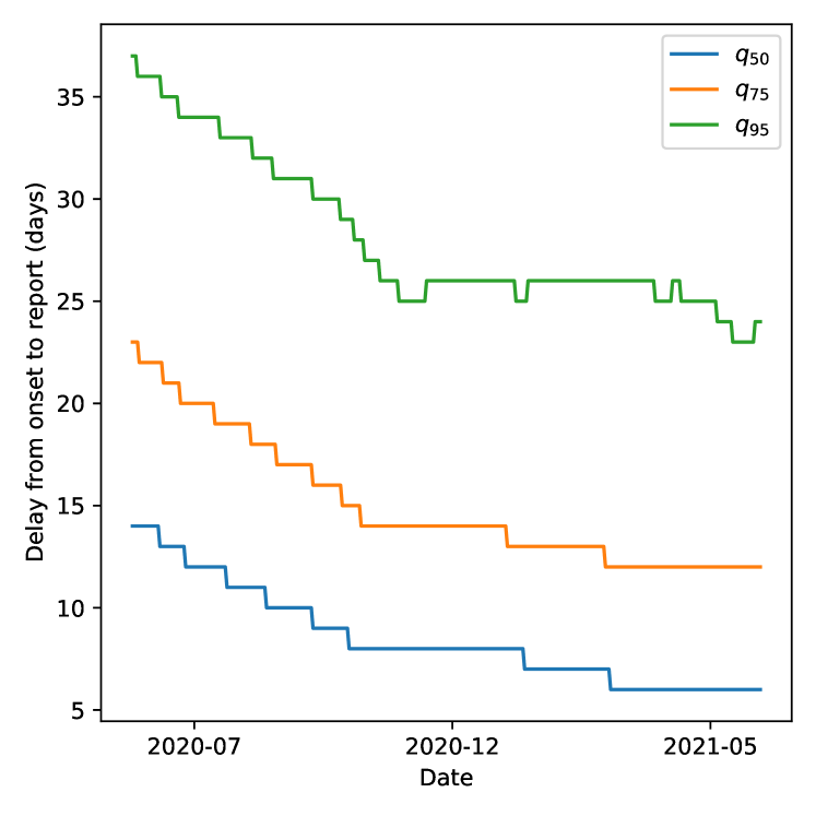
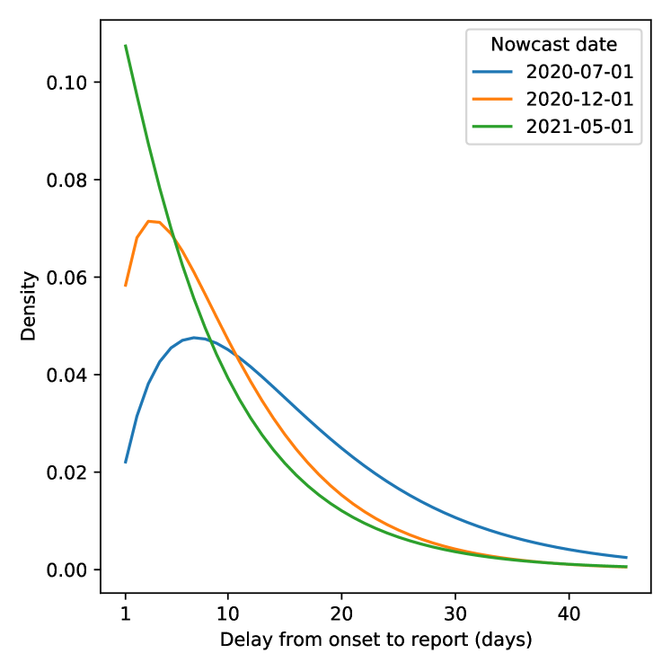
Figure 3: Top: quantiles of the estimated delay distribution returned by Algorithm 1 at the levels 50%, 75%, and 95%, as $t$ varies from June 1, 2020 to June 1, 2021. Bottom: estimated delay distributions overlaid for three nowcast dates within the same time interval.

We use only “recent” pairs of onset and report dates at time $t$ (whose onset date lies in $[t-2d+1,t]$) in order to adapt to the nonstationarity in reporting delays over time. The top panel in Figure 3 plots quantiles of the estimated delay distribution from Algorithm 1, as $t$ ranges from June 1, 2020 to June 1, 2021. We see sharp drops in all quantiles during the first half of this period, and then a more gradual decline over time. The bottom panel in the figure gives a qualitative sense of how the delay distribution estimates change in shape over time.

3.3 Defining Ground Truth

Given the estimated delay distributions over time from the previous subsection, we now describe how to estimate latent infections in the model (3). In short, we will solve one large optimization problem to perform deconvolution. To define the best possible retrospective estimates of latent infections over the period October 1, 2020 to June 1, 2021, which we will treat as ground truth in what follows (in the sense that they will be the point of comparison for all of our real-time estimates), we will perform deconvolution over a wider time period than the previously specified one in order to avoid any bias issues at the boundaries (where there is insufficient data for accurate deconvolution; more details are provided in the next section): our retrospective deconvolution runs from May 1, 2020 to August 28, 2021, a period we denote by $\mathcal{T}$, and uses case data published on August 30, 2021.

For location $\ell$, denote by $y_{\ell,t}$ and $x_{\ell,t}$ the number of new cases reported and number of new infections that onset at time $t$, respectively, per 100,000 people. Note that $y_{\ell,t},x_{\ell,t}$ obey (3), (4), because we have just rescaled the underlying counts here by a constant (in order to put them on the scale of rates), and recall, we assume that all locations have the same delay distribution (Assumption 3).

Given the delay distribution estimates from Algorithm 1, $\hat{p}_{t}=(\hat{p}_{t}(1),\ldots,\hat{p}_{t}(d))$ for $t\in\mathcal{T}$, we estimate the full vector $x_{\ell}=(x_{\ell,t})_{t\in\mathcal{T}}$ of latent infection rates across time, separately for each location $\ell$, by solving the problem:

$$\mathop{\mathrm{minimize}}_{x_{\ell}}\;\sum_{t\in\mathcal{T}}\bigg{(}y_{\ell,t}-\sum_{k=1}^{d}\hat{p}_{t}(k)\,x_{\ell,t-k}\bigg{)}^{2}+{}\\ \lambda\|D^{(4)}x_{\ell}\|_{1},$$ (5)

where $D^{(4)}$ is a matrix such that $D^{(4)}v$ gives all 4^th-order differences of a vector $v$, and $\|\cdot\|_{1}$ is the $\ell_{1}$ norm. Problem (5) could be called a trend-filtering-regularized least squares deconvolution problem. We solve it (as well as all related optimization problems in this paper) numerically with an adaption of the ADMM algorithm of Ramdas and Tibshirani (2016), detailed in Appendix A.

The solution $\hat{x}_{\ell}$ in problem (5) takes the form of a cubic piecewise polynomial (discrete spline) with adaptively chosen knots (Tibshirani, 2014, 2020). The tuning parameter $\lambda\geq 0$ controls its complexity, and we choose it using 3-fold cross-validation: we hold out every third value from training, and impute it by the average of the neighboring trained estimates; to compute the validation error, we reconvolve the full vector of imputed infections and measure against observed cases.

4 Real-Time Deconvolution

Real-time deconvolution refers to the the task of deconvolving case reports observed up until time $t$ to estimate latent infections up until $t$, repeatedly, as $t$ marches over the period of interest. We are particularly focused on estimating recent latent infections—nowcasting at a $k$-day lag, which means estimating at $t$ the latent infection rate at time $t-k$.

Compared to retrospective deconvolution, real-time deconvolution differs in two important ways. The first is that we are forced to work with provisional case data, subject to revision at times in the future, as discussed earlier in Section 2.1. All of our experiments in what follows use properly-versioned data that would have been available as of the nowcast date. We use the notation $y^{(t)}_{\ell,s}$ to reflect the reported case rate in location $\ell$ at time $s$ as of time $t$. Reported case data from JHU is available at a 1-day lag and therefore, as of time $t$, we only observe $y^{(t)}_{\ell,s}$ up through $s=t-1$ (we use analogous superscript notation for all auxiliary signals and estimates). This means we can only produce deconvolution estimates $\hat{x}^{(t)}_{\ell,s}$ up through $s=t-2$ (recall we exclude zero delays, in Assumption 2).

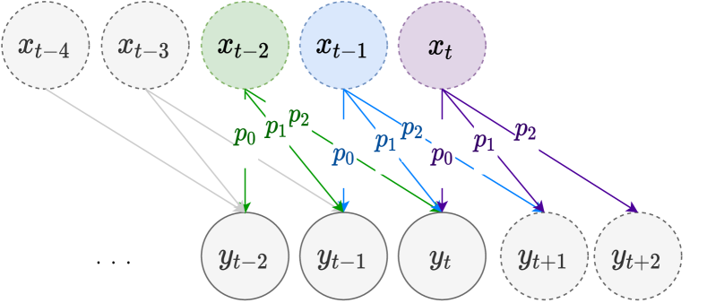
Figure 4: Illustration of right truncation with a delay distribution of length 3 (which is taken to be stationary for simplicity). At the nowcast time $t$, some “part” of the latent signal $x_{t}$ will appear in $y_{t+1},y_{t+2}$; likewise, some “part” of $x_{t-1}$ will appear in $y_{t+1}$.

The second issue of note, in real-time deconvolution, is right truncation: in nowcasting at lag $k$, where $k$ is small (compared to $d$), we are only able to carry out a “partial” deconvolution, as much of the needed information would come from case reports occurring in the future, past time the nowcast date $t$. Figure 4 gives an illustration. Thus, if we simply performed real-time deconvolution by solving the problem analogous to (5), using data that would have been available at time $t$,

$$\mathop{\mathrm{minimize}}_{x^{(t)}_{\ell}}\;\sum_{s<t}\bigg{(}y^{(t)}_{\ell,s}-\sum_{k=1}^{d}\hat{p}^{(t)}_{s}(k)\,x^{(t)}_{\ell,s-k}\bigg{)}^{2}+{}\\ \lambda\big{\|}D^{(4)}x^{(t)}_{\ell}\big{\|}_{1},$$ (6)

then we would find that the solution $\hat{x}^{(t)}_{\ell}=(\hat{x}^{(t)}_{\ell,s}:s<t)$ has highly volatile components for $s$ close to $t$.

The problem does not stop there; the truncation of data after the nowcast time $t$ also affects estimation of the delay distribution itself. Most rows in the line list with an onset date of $s=t-k$, for small $k$, will only have a report date (and thus not appear in the line list) until after time $t$. This means that the estimate $\hat{p}^{(t)}_{s}$ of $p_{s}$ given by the empirical distribution of all available line list data, with report date less than $t$, will be biased toward smaller lag values (i.e., it will place too little weight on larger lag values).

In the next two subsections, we work through each of these truncation issues in turn, by incorporating extra regularization around the right boundary into the criterion in (6), and estimating the delay distribution from truncated data using a Kaplan-Meier-like approach.

4.1 Incorporating Extra Regularization

We consider two forms of extra regularization to dampen the variability of trend filtering estimates toward the right boundary.

Natural Trend Filtering.

A natural cubic spline places additional regularity on top of the cubic spline, by maintaining that the function be linear beyond the left and right boundary points of the underlying domain. Natural trend filtering proceeds in a similar vein, but operating in the space of discrete splines; see Tibshirani (2020). Transporting this idea over to our real-time deconvolution problem (6), and applying it to the right boundary only, gives:

$$\mathop{\mathrm{minimize}}_{x^{(t)}_{\ell}}\; \sum_{s<t}\bigg{(}y^{(t)}_{\ell,s}-\sum_{k=1}^{d}\hat{p}^{(t)}_{s}(k)\,x^{(t)}_{\ell,s-k}\bigg{)}^{2}+{}$$ (7)

$$\hskip 100.0pt\hfill\lambda\big{\|}D^{(4)}x^{(t)}_{\ell}\big{\|}_{1}$$

$$\mathop{\mathrm{subject\,\,to}} \;\;x^{(\ell)}_{t}-2x^{(\ell)}_{t-1}+x^{(\ell)}_{t-2}=0.$$

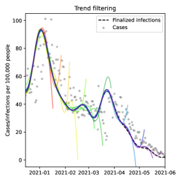
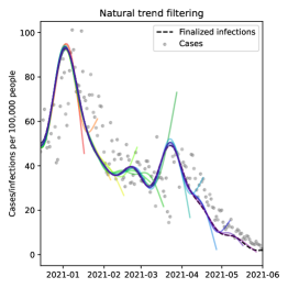
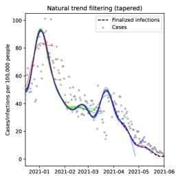
Figure 5: Comparison of boundary behavior for real-time deconvolution in New York, displayed for a sample of different nowcast dates (where each colored curve traces out the deconvolution estimates for a different nowcast date). The black dashed line indicates finalized infections, estimated roughly three months after June 1, 2021.

The left and middle panels of Figure 5 demonstrate the improvement that the additional constraints in (7) can have on the boundary estimates, particularly during periods of dynamic change in the underlying case trajectories.

Tapered Smoothing.

The right truncation phenomenon is not a binary one and there is increasingly less and less information available for deconvolution as we move the time index $s$ up toward the nowcast date $t$. Therefore, we design a second penalty to add to the criterion in (7) to gradually increase the amount of regularization accordingly:

$$\mathop{\mathrm{minimize}}_{x^{(t)}_{\ell}}\; \sum_{s<t}\bigg{(}y^{(t)}_{\ell,s}-\sum_{k=1}^{d}\hat{p}^{(t)}_{s}(k)\,x^{(t)}_{\ell,s-k}\bigg{)}^{2}+{}$$ (8)

$$\hskip 25.0pt\hfill\lambda\big{\|}D^{(4)}x^{(t)}_{\ell}\big{\|}_{1}+\gamma\big{\|}W^{(t)}D^{(1)}x^{(t)}_{\ell}\big{\|}_{2}^{2}$$

$$\mathop{\mathrm{subject\,\,to}} \;\;x^{(\ell)}_{t}-2x^{(\ell)}_{t-1}+x^{(\ell)}_{t-2}=0,$$

where $D^{(1)}v$ gives the first-order differences of a vector $v$, and $W^{(t)}$ is a diagonal matrix that is supported on the last $d$ diagonal entries, these being (in reverse order, starting with the last entry):

$$\frac{1}{\sqrt{\hat{F}^{(t)}_{t-1}(k)}},\;\;k=1,\dots,d,$$

where $\hat{F}^{(t)}_{t-1}$ is the cumulative distribution function (CDF) corresponding to the estimated delay distribution $\hat{p}^{(t)}_{t-1}$ at the most recent time $t-1$. The parameter $\gamma\geq 0$ controls the strength of the additional “tapered” penalty in (8), and we tune $\lambda,\gamma$ with a two-stage cross-validation procedure:

1. fix $\gamma=0$, and tune $\lambda$ using 3-fold cross-validation, as before;

2. fix $\lambda$ at the value in Step 1, and tune $\gamma$ using 7-fold forward-validation: for $s=t-2,\ldots,t-8$, we solve the deconvolution problem with a working nowcast date of $s$, linearly extrapolate to impute an estimate at $s+1$, and then we reconvolve the solution vector along with this imputed point and measure error against observed cases at time $s+1$; the validation error is obtained by averaging these errors over the iterations $s=t-2,\ldots,t-8$.

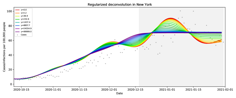
Figure 6: Effect of the tapered smoothing penalty, as we vary the corresponding tuning parameter $\gamma$, for a single real-time deconvolution example with on nowcast date February 1, 2021. The gray region highlights the components on which the tapered smoothing penalty acts.

Figure 6 displays the effect of varying $\gamma$ on the solution in (8), for a particular deconvolution example, to give a qualitative sense of the role of the tapered penalty. Furthermore, the right panel in Figure 5 demonstrates the benefit this penalty can provide in nowcasting.

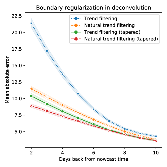
Figure 7: Comparing regularization approaches by MAE for nowcasting (the shaded bands here and henceforth, in all MAE figures, correspond to 95% bootstrap confidence intervals.) Both approaches for additional regularization give a huge improvement on trend filtering. The biggest improvement comes from combining the two approaches.

Lastly, and importantly, Figure 7 quantifies the improvement offered by the additional regularization mechanisms, in terms of mean absolute error (MAE) measured against finalized infections in nowcasting at a $k$-day lag, for each $k=2,\ldots,10$. This is averaged over all locations and every 10th nowcast date in the evaluation set. We see a considerable improvement in both the natural trend filtering and tapered smoothing modifications, with the biggest improvement occurring when the two are combined as in (8), and hence we stick with this framework in what follows.

4.2 Adjusting the Delay Distribution for Truncation

Now we propose an iterative adjustment to the empirical distribution of truncated line list data in order to overcome the truncation bias. To develop intuition, we first describe the problem using a simple abstraction, formulate a general solution, and then we translate this back over to our particular setting.

KM-Adjustment Under Truncation.

Suppose $p$ is a distribution that is supported on $\{1,\ldots,d\}$, and we observe independent random draws that we can partition into two sets: $\mathcal{D}_{1}$ and $\mathcal{D}_{2}$, where $\mathcal{D}_{2}$ contains draws from $p$ and $\mathcal{D}_{1}$ contains draws from $p$ conditional on the random variable lying in $[1,z_{1}]$, for a fixed $z_{1}\in\{1,\ldots,d\}$. Denote by $\hat{p}_{\mathcal{D}}$ the empirical distribution based on a data set $\mathcal{D}$. Clearly $\hat{p}_{\mathcal{D}_{2}}$ is unbiased for $p$, but $\hat{p}_{\mathcal{D}_{1}}$ is generally biased (it always places zero mass above $z_{1}$), and thus the pooled estimate $\hat{p}_{\mathcal{D}_{1}\cup\mathcal{D}_{2}}$ would be biased as well.

To build a more informed estimate based on the pooled sample, the intuition is as follows. First, observe that the only way we can estimate $p(k)$ for $k>z_{1}$ is by using $\mathcal{D}_{2}$. Then, this gives an estimate of $S(z_{1})=\sum_{k>z_{1}}p(k)$, the survival function of $p$ at $z_{1}$, and we can estimate $p(k)$ for $k\leq z_{1}$, denoting $Z\sim p$, by observing that

$$p(k)=\mathbb{P}(Z=k\,|\,Z\leq z_{1})(1-S(z_{1})).$$

where we estimate $\mathbb{P}(Z=k|Z\leq z_{1})$ using the empirical distribution over the set $\mathcal{D}_{1}\cup\mathcal{D}_{2}\cap[1,z_{1}]$. In other words, we construct our distribution estimate $\bar{p}$ using two steps:

1. define $\bar{p}(k)=\hat{p}_{\mathcal{D}_{2}}(k)$ for $k>z_{1}$, and also $\bar{S}(z_{1})=\sum_{k>z_{1}}\bar{p}(k)$;

2. define $\bar{p}(k)=\hat{p}_{\mathcal{D}_{0}}(k)(1-\bar{S}(z_{1}))$ for $k\leq z_{1}$, where we let $\mathcal{D}_{0}=\mathcal{D}_{1}\cup\mathcal{D}_{2}\cap[1,z_{1}]$.

We can readily generalize the above to a setting in which we observe $N$ data sets, with varying levels of truncation:

$$\text{$\mathcal{D}_{i}$ contains draws $Z\sim p\,|Z\leq z_{i}$, $i=1,\ldots,N$},$$ (9)

where $1\leq z_{1}<\cdots<z_{N}=d$, and we set $z_{0}=0$ for notational simplicity. To construct an estimate of $p$ based on all the samples, we proceed iteratively as before: first we estimate $p(k)$ for $k>z_{N-1}$ based on the data in $\mathcal{D}_{N}$, then we estimate $p(k)$ for $k\in(z_{N-2},z_{N-1}]$ based on data in $\mathcal{D}_{N-1}\cup\mathcal{D}_{2}\cap[1,z_{N-1}]$, and so on. Algorithm 2 spells out the procedure in full.

Input: Data sets and truncation limits $\mathcal{D}_{i}$ and $z_{i}$, for $1,\ldots,N$, as in (9).

Output: Estimated probabilities $\bar{p}(1),\ldots,\bar{p}(d)$.

1

2Initialize $\bar{S}(d)=0$.

3for $i=N,\ldots,1$ do

4       Set $\mathcal{D}_{0}=\bigcup_{j=i}^{N}D_{j}\cap[1,z_{i}]$.

5      Compute $\bar{p}(k)$, for $k\in(z_{i-1},z_{i}]$ based on the empirical distribution of data in $\mathcal{D}_{0}$ and an estimate of the survival function at $z_{i}$:

$$\bar{p}(k)=\hat{p}_{\mathcal{D}_{0}}(k)(1-\bar{S}(z_{i})),\;\;k\in(z_{i-1},z_{i}].$$

6      Compute an estimate of the survival function at $z_{i-1}$:

$$\bar{S}(z_{i-1})=\bar{S}(z_{i})+\sum_{k\in(z_{i-1},z_{i}]}\bar{p}(k).$$

7 end for

8

Return $\bar{p}(1),\ldots,\bar{p}(d)$.

Algorithm 2 Distribution estimation under sequential truncation

The algorithm just derived may be seen as Kaplan-Meier-like, in the sense that it is motivated by the decomposition

$$p(k)=\mathbb{P}(Z=k\,|\,Z\leq z_{i})(1-S(z_{i})),\;\;k\in(z_{i-1},z_{i}].$$

We use an unbiased plug-in estimate for each term in the product above based on the appropriate data. The Kaplan-Meier estimator has a similar plug-in foundation (Kaplan and Meier, 1958), so we refer to our approach as the KM-adjusted estimator of the distribution under truncation.

Application to CDC Line List.

Porting the last idea over to the CDC line list, we can use it to estimate the delay distribution at time $s$ using the line list as of time $t$. Note that if $s<t-d$ then we can still use Algorithm 1, as there is no truncation issue whatsoever. However, if $s\geq t-d$, then we would need to apply the KM-adjusted estimator, because we would be using the rows in the line list whose onset date is at or shortly before $s$, but are only able to see those whose report date is at most $t-1$ (thus would have been available at time $t$). After making this adjustment to the empirical distribution, we apply gamma smoothing as before. This is detailed in Algorithm 3.

Input: Nowcast time $t$, working onset time $s$, support size $d$, window size $w=2d$, truncated line list $\mathcal{D}^{(t)}$ with onset dates $a_{i}$ and report dates $b_{i}$ such that $b_{i}<t$.

Output: Estimated delay probabilities $\hat{p}^{(t)}_{s}(1),\ldots,\hat{p}^{(t)}_{s}(d)$.

1

2if $s<t-d$ then

3       Return probability estimates from Algorithm 1 (setting $t=s$ and $\mathcal{D}=\mathcal{D}^{(t)}$ in the notation of that algorithm).

4 end if

5

6Set $N=d-(t-s)+2$.

7for $i=1,\ldots,N-1$ do

8       Define

$$\mathcal{D}_{i} =\{b_{i}-a_{i}:a_{i}=s-i+1\}$$

$$z_{i} =t-s+i-2.$$

9 end for

10

11Define $\mathcal{D}_{N}=\{b_{i}-a_{i}:a_{i}\in(s-w,t-d)\}$ and $z_{N}=d$.

12Use Algorithm 2 (applied to $\mathcal{D}_{i}$, $z_{i}$, $i=1,\ldots,N$) to compute probability estimates $\bar{p}_{t}(1),\ldots,\bar{p}_{t}(d)$.

13Fit a gamma density to $\bar{p}_{t}(1),\ldots,\bar{p}_{t}(d)$ using the method of moments (matching the mean and variance).

Discretize this gamma density to the support set $\{1,\ldots,d\}$, call the result $\hat{p}_{t}(1),\ldots,\hat{p}_{t}(d)$, and return these probabilities.

Algorithm 3 Delay distribution estimation in real-time

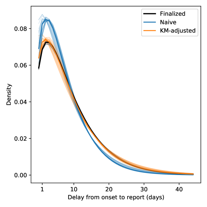
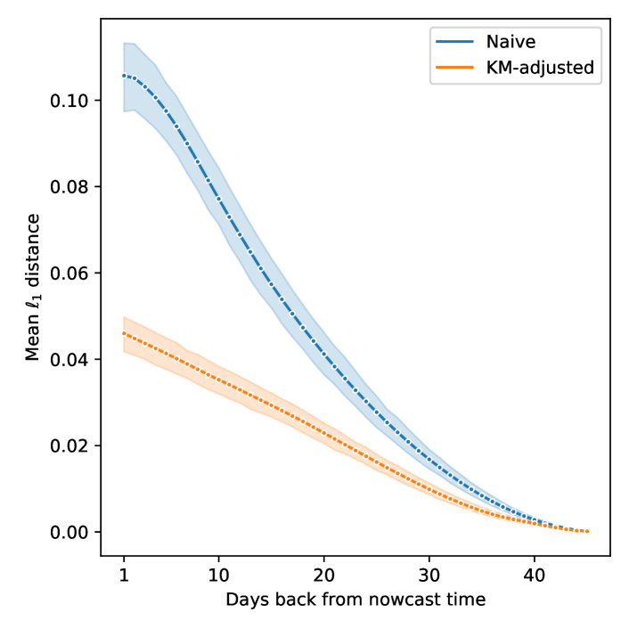
Figure 8: Top: estimated delay distributions overlaid for all nowcast dates in the month of November 2020, when $s=t-1$ (working onset date one day before the nowcast date). Bottom: mean $\ell_{1}$ distance to finalized estimate of the delay distribution, as a function of the lag $k=t-s$.

Figure 8 compares the KM-adjusted and naive estimates of the delay distribution, Algorithm 3 versus Algorithm 1 applied directly to $\mathcal{D}^{(t)}$, the line list available at each nowcast date $t$. In terms of $\ell_{1}$ distance, measured to the finalized delay distribution estimate computed retrospectively (based on the full untruncated line list), and averaged over all nowcast dates in the evaluation period, we see that the KM-adjustment greatly improves the accuracy at all lags $k=2,\ldots,10$ (where $k=t-s$, the difference between the nowcast and working onset dates).

4.3 Shortening the Deconvolution Window

Lastly, we investigate shortening the window used in the regularized deconvolution problem (8) so that we use only a window length of $w$ days before $t$:

$$\mathop{\mathrm{minimize}}_{x^{(t)}_{\ell}}\; \sum_{s\in[t-w,t)}\bigg{(}y^{(t)}_{\ell,s}-\sum_{k=1}^{d}\hat{p}^{(t)}_{s}(k)\,x^{(t)}_{\ell,s-k}\bigg{)}^{2}+{}$$ (10)

$$\hskip 25.0pt\hfill\lambda\big{\|}D^{(4)}x^{(t)}_{\ell}\big{\|}_{1}+\gamma\big{\|}W^{(t)}D^{(1)}x^{(t)}_{\ell}\big{\|}_{2}^{2}$$

$$\mathop{\mathrm{subject\,\,to}} \;\;x^{(\ell)}_{t}-2x^{(\ell)}_{t-1}+x^{(\ell)}_{t-2}=0,$$

As we are mainly interested in the components of the solution $\hat{x}^{(t)}_{s}$ for $s$ close to $t$, shortening the training window is computationally advantageous and should not change the behavior of the solution very much for $s$ close to $t$.

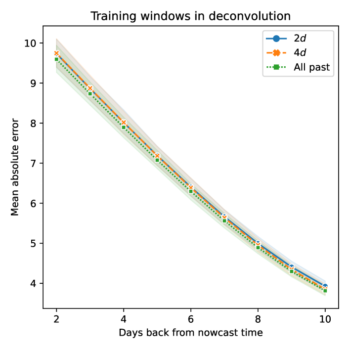
Figure 9: Comparing window lengths used in regularized deconvolution by MAE for nowcasting. The performance is very similar throughout.

Figure 9 compares (10) with $w=2d$, $w=4d$, and “all-past”, which is the original problem (8), in terms of mean absolute error (MAE) measured against finalized infections in nowcasting at a $k$-day lag, for each $k=2,\ldots,10$. This is averaged over all locations and every 10th nowcasting date in the evaluation set. The performance is basically identical for window lengths $2d$ and $4d$, and though all-past may appear to have the slightest advantage, this does not warrant the extra computation, hence in what follows we stick to (10) with a window length $w=2d$ as our real-time deconvolution estimator.

5 Leveraging Auxiliary Signals

The indicators enumerated in Section 2 have displayed impressive correlations to reported COVID-19 cases (Reinhart et al., 2021), and moreover, demonstrated an ability to improve the accuracy of case forecasting and hotspot prediction models (McDonald et al., 2021). In this section, we describe how to use each indicator to build a real-time sensor that estimates the latent infection rate, and how to fuse such estimates together into a single nowcast.

5.1 Sensor Models

At each prediction time $t$, for each location $\ell$, and for each of the five indicators (abbreviated CHNG-COVID, CHNG-CLI, DV-CLI, CTIS-CLIIC, and Google-AA), we will train a model to predict in real-time latent infections from indicator values. Let $\hat{x}^{(t)}_{\ell,s}$ denote the solution at time $s$ in problem (10), which represents our best estimate of the latent infection rate at time $s$ as of time $t$ from deconvolution of case rates alone.

We use $z^{i,(t)}_{\ell,s}$ to denote the value of indicator $i$ at time $s$ and location $\ell$, as of time $t$. We fit a simple linear model to predict latent infections from indicator values by solving

$$\mathop{\mathrm{minimize}}_{\beta_{0},\beta_{1}}\;\sum_{s=t-d}^{t-\tilde{k}_{i}}w^{(t)}_{s}\big{(}\hat{x}^{(t)}_{\ell,s}-\beta_{0}-\beta_{1}z^{i,(t)}_{\ell,s}\big{)}^{2},$$ (11)

which is a weighted linear regression over the time period $[t-d,t-\tilde{k}_{i}]$, where $\tilde{k}_{i}=\max\{k_{i},2\}$ and $k_{i}$ denotes the lag at which indicator $i$ is available. This is:

• $k_{i}=1$ for CTIS-CLIIC and Google-AA; and

• $k_{i}=4$ for the claims-based indicators, due to heavy revision or “backfill” over the first several days in the underlying claims data after an outpatient visit date (Reinhart et al., 2021).

Notice that, as defined, $\tilde{k}_{i}$ is the lag at which both the deconvolution estimate of infection rate and auxiliary signal $i$ are available, which is the data we need to fit the linear sensor model (response and covariate data, respectively).

The observation weights in (11) are given by

$$w^{(t)}_{t-k}=\hat{S}^{(t)}_{t-1}(k-1),\;\;k=1,\ldots,d.$$

Here $\hat{S}^{(t)}_{t-1}$ is the survival function of $\hat{p}^{(t)}_{t-1}$, the estimated delay distribution from the most recent time point $t-1$. We define $\hat{S}^{(t)}_{t-1}(1)=1$, corresponding to the exclusion of 0-day delays. This scheme upweights the more recent estimates (responses in the regression) of latent infections as they contain more timely information for nowcasting (assuming that the right-truncation bias has been effectively mitigated in the deconvolution step).

Given the solution $\hat{\beta}^{i,(t)}_{\ell,0},\hat{\beta}^{i,(t)}_{\ell,1}$ in (11), we then define a sensor—which is just a prediction from the fitted linear model—based on indicator $i$, for time $s$ and location $\ell$, as of time $t$, as:

$$\bar{x}^{i,(t)}_{\ell,s}=\hat{\beta}^{i,(t)}_{\ell,0}+\hat{\beta}^{i,(t)}_{\ell,1}\,z^{i,(t)}_{\ell,s}.$$ (12)

This sensor is available up until $s=t-k_{i}$. For the CTIS-CLIIC and Google-AA sensors, the lag is $k_{i}=1$, smaller than the inherent lag of 2 in the deconvolution estimate.

In brief, each sensor model takes a certain indicator and transforms it—using a location-specific and time-varying mapping—to the scale of local infection rates. While this mapping is simple (based on linear regression), it is also highly nontrivial, as it inherently accounts for geographic biases and nonstationarity.

Finally, in addition to defining sensors based on (11), (12) for each of the five auxiliary sensors, we also define a sixth sensor based on a 3^rd order autoregressive model trained on $\hat{x}^{(t)}_{\ell}=(\hat{x}^{(t)}_{\ell,s}:s<t)$. It is constructed exactly as in (11), (12) (same weights and same training window). Henceforth we abbreviate it AR(3).

5.2 Sensor Missingness

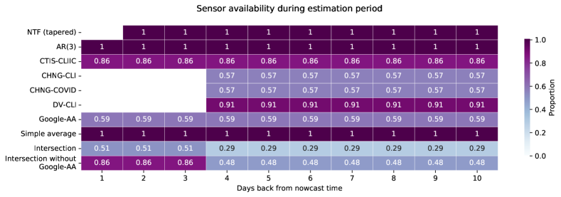
Figure 10: Proportion of observed (non-missing) values over the evaluation period from October 1, 2020 to June 1, 2021, and over all locations, as a function of lag $k=1,\ldots,10$. (NTF refers to the real-time deconvolution estimator, and simple average refers to the sensor fusion method that averages all available sensors.) The bottom two rows reflect the intersection of location-time pairs for which all data—deconvolution estimates and sensors—are available for that given lag, with and without including the Google-AA sensor, since this sensor has a large amount of individual missingness. Each intersection at each given lag $k$ is restricted to data whose latency is not greater than $k$. For example, the bottom leftmost cell computes the porportions of locations and dates at which AR(3), CTIS-CLIIC, and the simple average are concurrently available.

To be clear (11), (12) are to be implicitly understood as performed over observed (non-missing) indicator values. If an indicator value is missing at a particular location and time, then we drop it from the training set in (11), and do not produce a corresponding sensor value in (12). For a summary of missingness in the sensors, see Figure 10.

In general, an indicator will be missing when there is insufficient underlying data (from surveys, medical claims, etc.) to form a reliable signal value at a given location and time. However, the situation is different for the Google-AA indicator: here missingness occurs because the COVID-19 search trends data set is released after using a differential privacy layer (Bavadekar et al., 2020), and a missing value means that the level of noise added for privacy protection is high compared to the search count. Therefore we impute missing Google-AA signal values by zeros in our analysis; we do this unless the Google-AA signal was missing for a particular location and all times in the evaluation period, in which case we leave it as missing for this location entirely.

5.3 Sensor Fusion

Sensor fusion (SF), broadly speaking, refers to the process of assimilating data sources, each of which ideally contains complementary information, in order to produce more accurate estimates or predictions. SF falls into the general class of ensemble methods, and the sensors constructed in the previous section can be thought of as base learners, to be subsequently combined.

We consider the following five ensemble methods. In each case, we describe how to form the estimate at time $s$ and location $\ell$ as of time $t$. Though not explicitly stated, it is to be implicitly understood that all sensor values are as of time $t$ as well.

1. Simple average: the average of available sensors at time $s$ and location $\ell$.

2. Simple regression: the prediction from a linear regression model at time $s$ and location $\ell$, fit to available sensors over the training period at location $\ell$.

3. Ridge: the prediction from a ridge regression model at time $s$ and location $\ell$, fit to available sensors over the training period and over locations $j$ such that $j,\ell$ lie in the same U.S. state (including the state sensor itself).

4. Lasso: same as in the last item, but using the lasso instead of ridge regression.

5. KF-SF: the Kalman-Filter-inspired method for sensor fusion from Farrow (2016); Jahja et al. (2019), with covariance shrinkage, and operating on the geographical hierarchy within each U.S. state.

Methods 2–5 are trained on the most recent $2d$ time points, and 3–5 are tuned using 7-fold forward validation, where we allow them to choose a lag-specific tuning parameter. Methods 1–2 are “simple” in the sense that for nowcasting at a location $\ell$ they use sensors from $\ell$ only. Methods 3–5 are more sophisticated in that they pool information across locations within the same state.

The KF-SF method requires a proper geographical hierarchy and thus we create “rest-of-state” jurisdictions by aggregating the remaining counties (outside of the top 200 counties nationally) within each state, and to run KF-SF, we create an AR(3) sensor at these rest-of-state locations (since one sensor at each location is sufficient). It is worth noting that, as shown in Jahja et al. (2019), KF-SF bears a close connection to ridge in Model 4: it is in fact equivalent to a modified ridge optimization problem that imposes additional linear constraints.

6 Evaluation

We now evaluate nowcasting performance over all locations and all but every 10th nowcasting date in our evaluation period from October 1, 2020 to June 1, 2021. (We do this because it gives us a “pure” test set, since every 10th nowcasting date was already used to choose the real-time deconvolution methodology in Section 4.) As before, we compare to finalized estimates of infection rates computed via retrospective deconvolution, as in Section 3.

For the purposes of making fair comparisons, in every analysis (figure) that we present, we only aggregate over the intersection of nowcasts dates and locations at which the particular estimates under consideration—coming from real-time deconvolution, individual sensor models, or sensor fusion—are all available. Abiding by this rule leads us to examine several different ways of stratifying results, as the full intersection is fairly sparse (see the second-to-last row in Figure 10). In particular, we consider the following two dimensions used to define strata:

• inclusion of Google-AA or not;

• inclusion of all claims-based sensors (CHNG-CLI, CHNG-COVID, and DV-CLI) or not.

In what follows, we first examine the performance of individual sensor models and a certain sensor fusion method (the simple average) compared to real-time deconvolution, and then examine the relative performance of the different sensor fusion methods.

6.1 Performance of Sensors and Sensor Fusion

We begin by comparing the MAE of nowcasts from natural trend filtering (NTF) using tapered smoothing, as in (10) (the real-time deconvolution estimator chosen based on the analysis in Section 4) to those from individual sensor models and the simple average sensor fusion method. Despite its simplicity, the simple average appears to be the best-performing sensor fusion method overall (details in the next subsection), and so we stick with it as the de facto sensor fusion method in this subsection. The results here do not include Google-AA; results including Google-AA are shown in Appendix B.

Figure 11 displays the MAE from various methods as a function of lag $k$. The top and bottom panels do not and do include the claims-based sensors, respectively. In either case, we see that up until lag 6, all sensors outperform the real-time deconvolution estimate from NTF. The simple average of all sensors improves accuracy even further, and achieves the best MAE for all lags up through lag 6. We recall that NTF (with tapered smoothing) itself already provides a huge increase in accuracy over the more naive method for real-time deconvolution given by applying trend filtering without extra boundary regularization (Figure 7). At lag 7, the NTF estimate catches up to about equal accuracy, and then surpasses sensor fusion and all sensors in accuracy at lag 8 and onward. An interpretation for this: right truncation ceases to be a significant problem past lag 7, and thus we are better off performing deconvolution directly in order to estimate infections more than a week into the past.

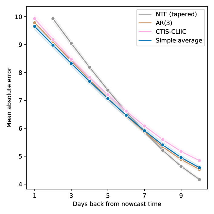
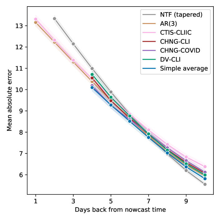
Figure 11: Comparing NTF to individual sensor models and the simple average sensor fusion method by MAE for nowcasting. The top panel excludes the claims-based sensors, whereas the bottom includes them. For lags smaller than 7, all methods improve upon NTF (with tapered smoothing), with simple average being the best among them.

Figure 12 displays the empirical distributions of ranks of nowcast errors coming from each method, computed with respect to each other, over common nowcast tasks (defined by a location-date-lag triplet). For example, in a particular nowcast task, we assign a rank of 1 to the method with the smallest absolute error for that nowcast task. The top panel again excludes claims-based signals, and the bottom panel includes them. The striking feature in either panel, particularly the bottom panel, is that the simple average has a highly distinctive distribution of ranks—it is rarely the best method, but never the worst. While this is not particularly surprising (averaging random variables tends to be variance-reducing, as long as the variables are not too correlated), it also points to a key property of sensor fusion—a certain kind of robustness, beyond accuracy.

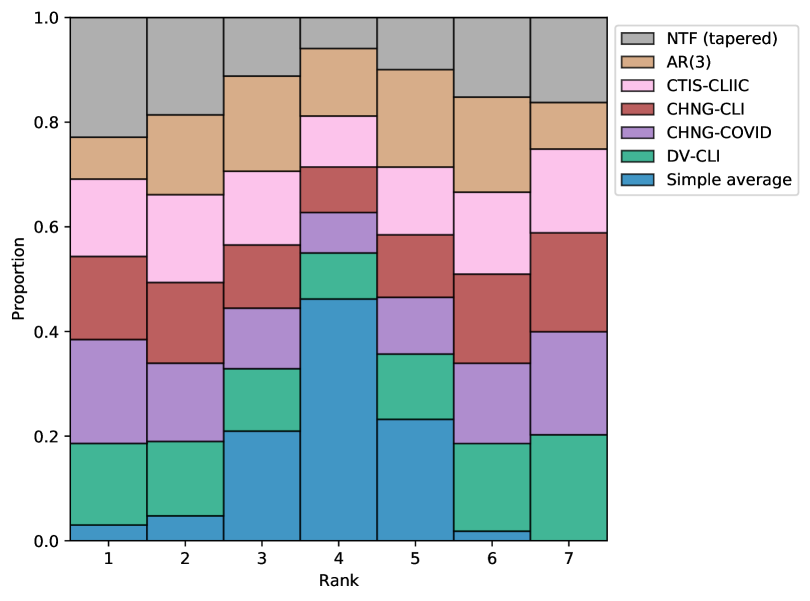
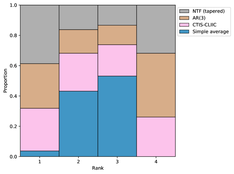
Figure 12: Comparing NTF to individual sensor models and the simple average sensor fusion method by relative ranks over common nowcast tasks. The top panel excludes all claims-based sensors and considers lags 1–5, whereas the bottom panel includes them and considers lags 4–9 (the first 5 lags at which all methods are available, in either case). The simple average exhibits striking consistency: it is rarely the best, but also never the worst.

6.2 Relative Performance of Sensor Fusion Methods

We now compare the various sensor fusion methods to each other. The results here do not include claims-based signals; results including claims-based signals are shown in Appendix B. Figure 13 displays the MAE of the various sensor fusion estimates, but divided up into three panels, defined by averaging over small, medium, and large states (the figure caption provides more details). Recall that for the lasso, ridge, and KF-SF approaches, a model in a particular county is fit using the sensors from other counties in the same state. Larger states have more pooling of information across locations and present a greater potential for gains in accuracy. We see that the simple average method is typically the best sensor fusion method at each lag, but for medium and large states, KF-SF catches up with it and is just about as accurate.

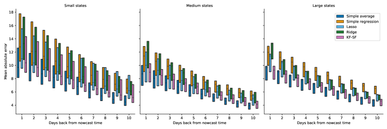
Figure 13: Comparing sensor fusion methods by boxenplots of nowcasting errors (each box conveys the level 25%, 50%, and 75% quantiles of the absolute error distribution.) The three panels average over small (containing less than 5 locations), medium (between 5 and 14 locations), and large (more than 15 locations) states. Simple average performs generally the best throughout, but KF-SF catches up for medium and large states.

Figure 14 displays the relative ranking of sensor fusion methods. The simple average and KF-SF methods appear the most favorable (often the best, and less so the worst), followed by lasso, then ridge, and lastly simple regression (most often the worst).

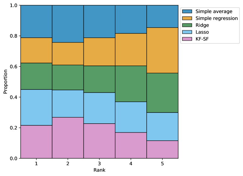
Figure 14: Comparing sensor fusion methods by relative ranks over common nowcast tasks, and considering only lags 1–5. The simple average and KF-SF methods consistently perform in the top half, while simple regression is most often the worst.

7 Discussion

In this work, we proposed, implemented, and evaluated a framework for real-time estimation of new symptomatic COVID-19 infections from case reports. At time $t$, in order to nowcast the infection rate at time $t-k$ (for small values of $k$, such as $k=1,2,\ldots$), the main steps are to:

1. estimate a symptom-onset-to-case-report delay distribution using the most recent data available in a line list provided by the CDC;

2. perform regularized deconvolution on the most recent case data available from JHU CSSE;

3. update models to track recent infection rates from various auxiliary signals (based on COVID-related data from medical insurance claims, online surveys, and Google searches), and fuse together the predictions from these models in order to stabilize recent estimates of infection rates.

In each step, we proposed methodological advances that improved the accuracy of our nowcasts, when measured against finalized infection rate estimates obtained by retrospective deconvolution (using data that would have only been available months later). While using auxiliary signals (step 3) did help in terms of accuracy and robustness, the additional regularization devices that we incorporated into real-time deconvolution (step 2) ended up providing the biggest benefit to accuracy.

To reiterate, we purposely defined our target of estimation to be symptomatic infections that would eventually show up in public health reports, allowing us to focus on developing and testing tools for real-time deconvolution and sensor fusion, with minimal assumptions (e.g., without a mechanistic model for disease spread). Estimating the number of true symptomatic infections at any point in time—whether or not they will appear in case reports—is of course a much harder problem. However, our methodology may be seen as a contribution toward solving this larger problem in real-time; moreover, some simple post hoc corrections could be applied to our real-time estimates in order to adjust for confounding. For example, if $a_{\ell,t}$ is the fraction of untested symptomatic infections in location $\ell$ at at time $t$, which (say) is estimated from external data sources, then we could just multiply each element $\hat{p}^{(t)}_{\ell,s}$ of the delay distribution used in (10) by $b_{\ell,t}=1/(1-a_{\ell,t})$ in order to estimate all symptomatic infections from case reports. Due to the way we have set up the deconvolution problem (cross-validating over optimal choices of tuning parameters), this would be essentially equivalent to post-mulitplying the nowcast $\hat{x}^{(t)}_{\ell,s}$ we already produce by $b_{\ell,t}$.

We finish by describing a few directions for future work.

Post Hoc Smoothing.

As we saw in Section 6, sensor fusion provides a real-time improvement on pure deconvolution up until about a 10-day lag, and past that point, the deconvolution estimates appear stable enough that sensor fusion becomes unnecessary. While the quantative benefit of sensor fusion for small lags is clear, sensor fusion is also lacking in the following qualitative aspect: its estimates do not always appear visually smooth across time (this is because the sensors themselves need not be smooth over time, and furthermore, sensor fusion may end up using a different subset of sensors at each lag, creating additional jaggedness). Post smoothing techniques would be worth investigating here, to aid visual consumption.

$R_{t}$ Estimation.

The instantaneous reproductive number $R_{t}$, the average number of secondary infections at time $t$ generated from a primary infection in the past, is a useful and interpretable parameter that reflects the dynamics of epidemic growth in a population. In the SIR model, the instantaneous reproductive number $R_{t}$ and growth rate $r_{t}$ at time $t$ obey the following relationship:

$$R_{t}\approx 1+\frac{r_{t}}{\gamma},$$

where $\gamma$ denotes the recovery rate in the SIR model. While this is well-known in the literature on mathematical modeling of epidemics (and is exact under local exponential growth; see, e.g., Wallinga and Lipsitch (2007)), its use in the presence of confounding seems to be underexplored and potentially undervalued. If $I_{t}$ denotes the number of new infections at $t$, then using a simple discrete difference approximation to $r_{t}$ leads to:

$$R_{t}\approx 1+\frac{1}{\gamma}\bigg{(}\frac{I_{t+1}}{I_{t}}-1\bigg{)}.$$

A similar though not identical approximation is given in Bettencourt and Ribeiro (2008), where $I_{t+1}/I_{t}-1$ is replaced by $\log(I_{t+1}/I_{t})$. Critically, incident infections only enter right-hand side above as a ratio of values adjacent in time, and thus if we are only able to estimate this up to an unknown multiplicative factor (due to confounding), then this factor approximately cancels in the ratio as long as it is slowly varying in time. In slightly more detail (and for simplicity, considering just a single location), suppose as before that a fraction $a_{t}$ of infections go untested at time $t$. Then $I_{t}=b_{t}x_{t}$ where $x_{t}$ is the number of new infections at time $t$ that show up in case reports (i.e., the focus of this paper) and $b_{t}=1/(1-a_{t})$. From the previous display,

$$R_{t}\approx 1+\frac{1}{\gamma}\bigg{(}\frac{b_{t+1}x_{t+1}}{b_{t}x_{t}}-1\bigg{)}\approx 1+\frac{1}{\gamma}\bigg{(}\frac{x_{t+1}}{x_{t}}-1\bigg{)},$$

where the last approximation is motivated by an additional assumption the untested fraction varies slowly over time (so $b_{t+1}/b_{t}\approx 1$). This shows that estimates of $x_{t}$ can produce approximately unconfounded estimates of $R_{t}$, even though $x_{t}$ is itself confounded due to a lack of universal testing. This is true both in the retrospective and real-time sense, and will be the topic of future study.

Evaluation via Reconvolution.

An important avenue for evaluating our methodology (beyond evaluating against finalized infection rate estimates, as we do in this paper), would be to reconvolve our real-time nowcasts of infection rates forward in time in order to predict future case rates, and evaluate these predictions against finalized case reporting data. Making and evaluating point predictions would be relatively straightforward, however, distributional forecasts are currently the standard in epidemiological forecasting (and also in COVID-19 forecasting), and adding a distributional layer to our nowcasts (and propagating this through the convolution operator) requires substantial new developments, and we leave it to future work.

[Acknowledgments] The authors are grateful to Logan Brooks, Roni Rosenfeld, James Sharpnack, Sam Abbott, Joel Hellewell, and Sebastian Funk for several early insightful conversations.

MJ was supported by a fellowship from the Center for Machine Learning and Health at Carnegie Mellon. AC and RJT were supported by a gift from Google.org.

Appendix A ADMM for Solving Deconvolution Problems

Here we give details on the ADMM approach used to solve the regularized least squares deconvolution problems in Sections 3 and 4. We first focus on problem (5), and then we discuss the modifications needed when incorporating extra regularization for real-time deconvolution as in (10). To simplify notation, we will henceforth drop the subscript dependnece of all quantities on the location $\ell$, as well as the superscript dependence on the nowcast date $t$ for the real-time problems.

We also use $\hat{P}$ to denote the (Toeplitz) convolution matrix with rows determined by $\hat{p}_{s}$, $s<t$, i.e., such that for any vector $x$ (of appropriate dimension)

$$(\hat{P}x)_{s}=\sum_{k=1}^{d}\hat{p}_{k}x_{s-k}.$$

(We leave the dimensions of $\hat{P}$ and $x$ here purposely ambiguous, which should always be clear from the context anyway; this allows us to borrow similar notation across problems with different underlying dimensions.) Thus we can rewrite (5) as

$$\mathop{\mathrm{minimize}}_{x}\;\|y-\hat{P}x\|_{2}^{2}+\lambda\|D^{(4)}x\|_{1}.$$

To apply ADMM, we must introduce auxiliary variables, and as in Ramdas and Tibshirani (2016), we use the following “specialized” decomposition (which improves the convergence speed):

$$\mathop{\mathrm{minimize}}_{x}\; \|y-\hat{P}x\|_{2}^{2}+\lambda\|D^{(1)}\alpha\|_{1}$$

$$\mathop{\mathrm{subject\,\,to}} \;\;\alpha=D^{(3)}x,$$

where we used the recursive nature of the difference operators, writing the 4^th-order operator as a product of the 1^st- and 3^rd-order operators: $D^{(4)}=D^{(1)}D^{(3)}$. The above problem gives rise to the augmented Lagrangian:

$$\mathcal{L}(x,\alpha,u)=\|y-\hat{P}x\|_{2}^{2}+\lambda\|D^{(1)}\alpha\|_{1}+{}\\ \rho\|\alpha-D^{(3)}x+u\|_{2}^{2}-\rho\|u\|_{2}^{2},$$

which corresponds to following ADMM updates, writing $D=D^{(3)}$ for brevity:

$$x \leftarrow(\hat{P}^{T}\hat{P}+\rho D^{T}D)^{-1}\big{(}\hat{P}^{T}y+\rho D^{T}(\alpha+u)\big{)}$$

$$\alpha \leftarrow\mathop{\mathrm{argmin}}_{z}\;\|Dx-u-z\|_{2}^{2}+\frac{\lambda}{\rho}\|D^{(1)}\alpha\|_{1}$$

$$u \leftarrow u+\alpha-Dx.$$

The $\alpha$-update here requires solving a 1-dimensional fused lasso problem, which can be done in linear-time with the dynamic programming approach of Johnson (2013). The $x$-update is more expensive than in pure trend filtering (with no convolution operator) but owing to the bandedness of $\hat{P}$ (and $D$, though the bandwidth $d$ of $\hat{P}$ dominates), it can still be solved in $O(nd)$ operations. Further, in this and all applications of ADMM, we follow the recommendation of Ramdas and Tibshirani (2016) and set the Lagrangian parameter equal to the tuning parameter, $\rho=\lambda$.

As for the two extensions presented in (10), the natural trend filtering constraints can be be enforced by introducing a linear interpolant matrix as described in Section 11.2 of Tibshirani (2020). This effectively replaces the convolution matrix $\hat{P}$ and the 3^rd difference operator $D$, in the ADMM steps above, by $\tilde{P}$ and $\tilde{D}$, respectively, which are given by right multiplying $P$ and $D$ by the interpolant matrix.

Moreover, the additional tapered smoothing term can be pushed into the augmented Lagrangian, and only alters the $x$-update, now becoming:

$$x\leftarrow(\tilde{P}^{T}\tilde{P}+\gamma M^{T}M+\rho\tilde{D})^{-1}\cdot{}\\ \big{(}\tilde{P}^{T}y+\rho\tilde{D}^{T}(\alpha+u)\big{)},$$

where $M$ is the matrix $W^{(t)}D^{(1)}$ in the tapered penalty in (10) times the linear interpolant matrix.

Appendix B Additional Evaluation Results

Figures 15 and 16 are analogous to Figures 11 and 12, but with the inclusion of the Google-AA sensor. Similarly, Figures 17 and 18 are the counterparts to Figures 13 and 14, but with the inclusion of claims-based sensors.

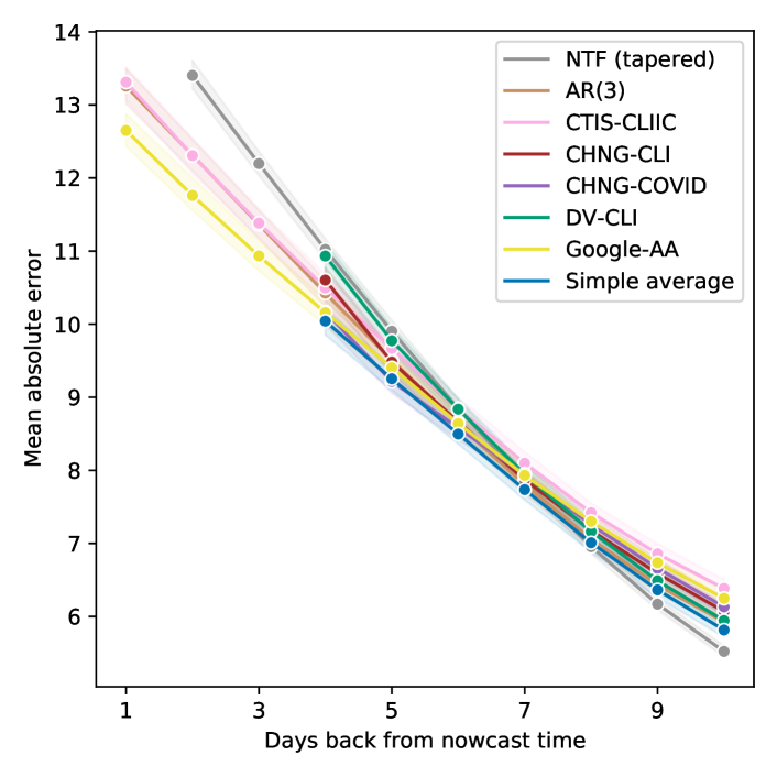
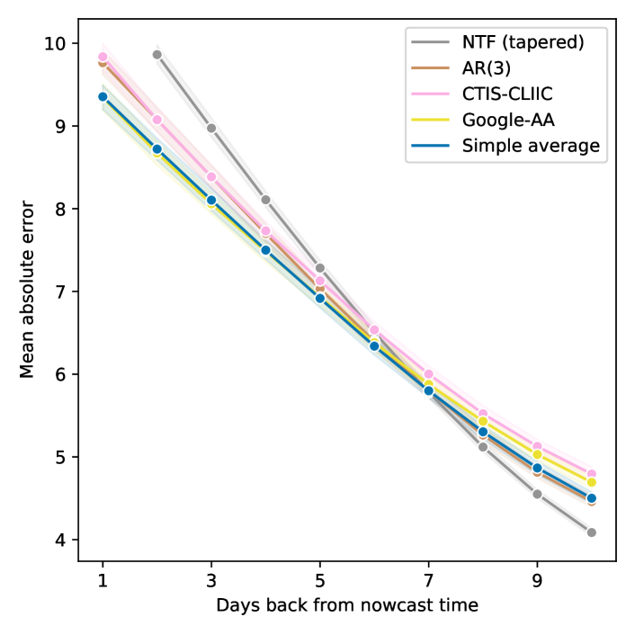
Figure 15: As in Figure 11, but including Google-AA.

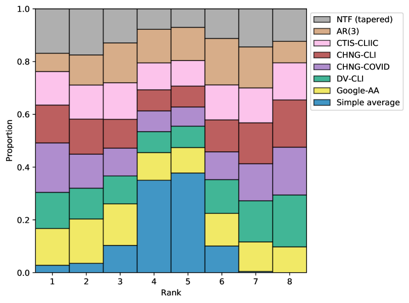
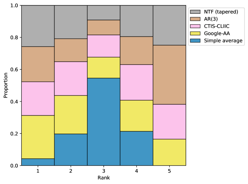
Figure 16: As in Figure 12, but including Google-AA.

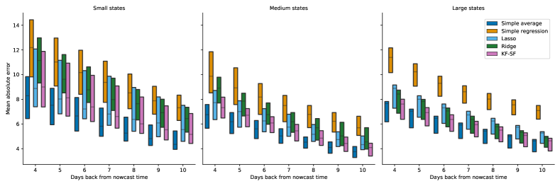
Figure 17: As in Figure 13, but including claims-based signals.

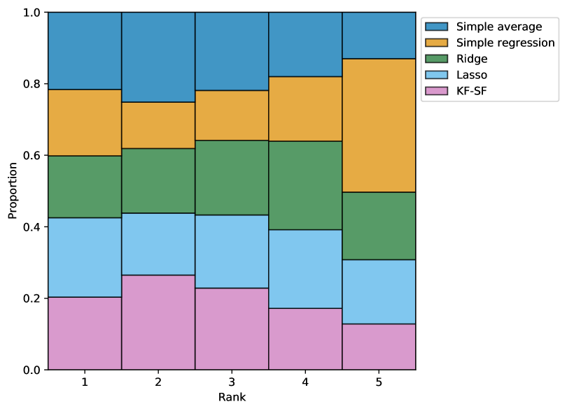
Figure 18: As in Figure 14, but including claims-based signals.

References

- Abbott et al. (2020) {barticle}[author] \bauthor\bsnmAbbott, \bfnmSam\binitsS., \bauthor\bsnmHellewell, \bfnmJoel\binitsJ., \bauthor\bsnmThompson, \bfnmRobin N\binitsR. N., \bauthor\bsnmSherratt, \bfnmKatharine\binitsK., \bauthor\bsnmGibbs, \bfnmHamish P\binitsH. P., \bauthor\bsnmBosse, \bfnmNikos I\binitsN. I., \bauthor\bsnmMunday, \bfnmJames D\binitsJ. D., \bauthor\bsnmMeakin, \bfnmSophie\binitsS., \bauthor\bsnmDoughty, \bfnmEmma L\binitsE. L., \bauthor\bsnmChun, \bfnmJune Young\binitsJ. Y., \bauthor\bsnmChan, \bfnmYung-Wai Desmond\binitsY.-W. D., \bauthor\bsnmFinger, \bfnmFlavio\binitsF., \bauthor\bsnmCampbell, \bfnmPaul\binitsP., \bauthor\bsnmEndo, \bfnmAkira\binitsA., \bauthor\bsnmPearson, \bfnmCarl A B\binitsC. A. B., \bauthor\bsnmGimma, \bfnmAmy\binitsA., \bauthor\bsnmRussell, \bfnmTim\binitsT., \bauthor\bsnmCMMID COVID modelling group, \bauthor\bsnmFlasche, \bfnmStefan\binitsS., \bauthor\bsnmKucharski, \bfnmAdam J\binitsA. J., \bauthor\bsnmEggo, \bfnmRosalind M\binitsR. M. and \bauthor\bsnmFunk, \bfnmSebastian\binitsS. (\byear2020). \btitleEstimating the time-varying reproduction number of SARS-CoV-2 using national and subnational case counts. \bjournalWellcome Open Research \bvolume5. \endbibitem
- Ackley et al. (2020) {barticle}[author] \bauthor\bsnmAckley, \bfnmAarah F\binitsA. F., \bauthor\bsnmPilewski, \bfnmSarah\binitsS., \bauthor\bsnmPetrovic, \bfnmVladimir S\binitsV. S., \bauthor\bsnmWorden, \bfnmLee\binitsL., \bauthor\bsnmMurray, \bfnmErin\binitsE. and \bauthor\bsnmPorco, \bfnmTravis C\binitsT. C. (\byear2020). \btitleassessing the utility of a smart thermometer and mobile application as a surveillance tool for influenza and influenza-like illness. \bjournalHealth Informatics Journal \bvolume26 \bpages2148–2158. \endbibitem
- Bavadekar et al. (2020) {bunpublished}[author] \bauthor\bsnmBavadekar, \bfnmShailesh\binitsS., \bauthor\bsnmDai, \bfnmAndrew\binitsA., \bauthor\bsnmDavis, \bfnmJohn\binitsJ., \bauthor\bsnmDesfontaines, \bfnmDamien\binitsD., \bauthor\bsnmEckstein, \bfnmIlya\binitsI., \bauthor\bsnmEverett, \bfnmKatie\binitsK., \bauthor\bsnmFabrikant, \bfnmAlex\binitsA., \bauthor\bsnmFlores, \bfnmGerardo\binitsG., \bauthor\bsnmGabrilovich, \bfnmEvgeniy\binitsE., \bauthor\bsnmGadepalli, \bfnmKrishna\binitsK., \bauthor\bsnmGlass, \bfnmShane\binitsS., \bauthor\bsnmHuang, \bfnmRayman\binitsR., \bauthor\bsnmKamath, \bfnmChaitanya\binitsC., \bauthor\bsnmKraft, \bfnmDennis\binitsD., \bauthor\bsnmKumok, \bfnmAkim\binitsA., \bauthor\bsnmMarfatia, \bfnmHinali\binitsH., \bauthor\bsnmMayer, \bfnmYael\binitsY., \bauthor\bsnmMiller, \bfnmBenjamin\binitsB., \bauthor\bsnmPearce, \bfnmAdam\binitsA., \bauthor\bsnmPerera, \bfnmIrippuge Milinda\binitsI. M., \bauthor\bsnmRamachandran, \bfnmVenky\binitsV., \bauthor\bsnmRaman, \bfnmKarthik\binitsK., \bauthor\bsnmRoessler, \bfnmThomas\binitsT., \bauthor\bsnmShafran, \bfnmIzhak\binitsI., \bauthor\bsnmShekel, \bfnmTomer\binitsT., \bauthor\bsnmStanton, \bfnmCharlotte\binitsC., \bauthor\bsnmStimes, \bfnmJacob\binitsJ., \bauthor\bsnmSun, \bfnmMimi\binitsM., \bauthor\bsnmWellenius, \bfnmGregory\binitsG., \bauthor and \bauthor\bsnmZoghi, \bfnmMasrour\binitsM. (\byear2020). \btitleGoogle COVID-19 search trends symptoms dataset: Anonymization process description. \bnotearXiv: 2009.01265. \endbibitem
- Bettencourt and Ribeiro (2008) {barticle}[author] \bauthor\bsnmBettencourt, \bfnmLuis MA\binitsL. M. and \bauthor\bsnmRibeiro, \bfnmRuy M\binitsR. M. (\byear2008). \btitleReal time Bayesian estimation of the epidemic potential of emerging infectious diseases. \bjournalPLOS ONE \bvolume3 \bpagese2185. \endbibitem
- Brooks (2020) {bphdthesis}[author] \bauthor\bsnmBrooks, \bfnmLogan C\binitsL. C. (\byear2020). \btitlePancasting: Forecasting epidemics from provisional data, \btypePhD thesis, \bpublisherCarnegie Mellon University. \endbibitem
- Brownstein, Freifeld and Madoff (2009) {barticle}[author] \bauthor\bsnmBrownstein, \bfnmJohn S\binitsJ. S., \bauthor\bsnmFreifeld, \bfnmClark C\binitsC. C. and \bauthor\bsnmMadoff, \bfnmLawrence C\binitsL. C. (\byear2009). \btitleDigital disease detection — harnessing the web for public health surveillance. \bjournalNew England Journal of Medicine \bvolume360 \bpages2153–2157. \endbibitem
- Carlson et al. (2013) {barticle}[author] \bauthor\bsnmCarlson, \bfnmSandra J\binitsS. J., \bauthor\bsnmDalton, \bfnmCraig B\binitsC. B., \bauthor\bsnmButler, \bfnmMichelle T\binitsM. T., \bauthor\bsnmFejsa, \bfnmJohn\binitsJ., \bauthor\bsnmElvidge, \bfnmElissa\binitsE. and \bauthor\bsnmDurrheim, \bfnmDavid N\binitsD. N. (\byear2013). \btitleFlutracking weekly online community survey of influenza-like illness annual report 2011 and 2012. \bjournalCommunicable diseases intelligence quarterly report \bvolume37 \bpagesE398–406. \endbibitem
- Charu et al. (2017) {barticle}[author] \bauthor\bsnmCharu, \bfnmVivek\binitsV., \bauthor\bsnmZeger, \bfnmScott\binitsS., \bauthor\bsnmGog, \bfnmJulia\binitsJ., \bauthor\bsnmBjørnstad, \bfnmOttar N.\binitsO. N., \bauthor\bsnmKissler, \bfnmStephen\binitsS., \bauthor\bsnmSimonsen, \bfnmLone\binitsL., \bauthor\bsnmGrenfell, \bfnmBryan T.\binitsB. T. and \bauthor\bsnmViboud, \bfnmCécile\binitsC. (\byear2017). \btitleHuman mobility and the spatial transmission of influenza in the United States. \bjournalPLOS Computational Biology \bvolume13 \bpages1–23. \endbibitem
- Chitwood et al. (2021) {bunpublished}[author] \bauthor\bsnmChitwood, \bfnmMelanie H\binitsM. H., \bauthor\bsnmRussi, \bfnmMarcus\binitsM., \bauthor\bsnmGunasekera, \bfnmKenneth\binitsK., \bauthor\bsnmHavumaki, \bfnmJoshua\binitsJ., \bauthor\bsnmPitzer, \bfnmVirginia E\binitsV. E., \bauthor\bsnmSalomon, \bfnmJoshua A\binitsJ. A., \bauthor\bsnmSwartwood, \bfnmNicole\binitsN., \bauthor\bsnmWarren, \bfnmJoshua L\binitsJ. L., \bauthor\bsnmWeinberger, \bfnmDaniel M\binitsD. M. and \bauthor\bsnmCohen, \bfnmTed\binitsT. (\byear2021). \btitleReconstructing the course of the COVID-19 epidemic over 2020 for US states and counties: results of a Bayesian evidence synthesis model. \bdoi10.1101/2020.06.17.20133983 \endbibitem
- Cori et al. (2013) {barticle}[author] \bauthor\bsnmCori, \bfnmAnne\binitsA., \bauthor\bsnmFerguson, \bfnmNeil M.\binitsN. M., \bauthor\bsnmFraser, \bfnmChristophe\binitsC. and \bauthor\bsnmCauchemez, \bfnmSimon\binitsS. (\byear2013). \btitleA new framework and software to estimate time-varying reproduction numbers during epidemics. \bjournalAmerican Journal of Epidemiology \bvolume178 \bpages1505–1512. \endbibitem
- Debeye and Van Riel (1990) {barticle}[author] \bauthor\bsnmDebeye, \bfnmH. W. J.\binitsH. W. J. and \bauthor\bsnmVan Riel, \bfnmP.\binitsP. (\byear1990). \btitle-norm deconvolution. \bjournalGeophysical Prospecting \bvolume38 \bpages381–403. \endbibitem
- Dong, Du and Gardner (2020) {barticle}[author] \bauthor\bsnmDong, \bfnmEnsheng\binitsE., \bauthor\bsnmDu, \bfnmHongru\binitsH. and \bauthor\bsnmGardner, \bfnmLauren\binitsL. (\byear2020). \btitleAn interactive web-based dashboard to track COVID-19 in real time. \bjournalThe Lancet Infectious Diseases \bvolume20 \bpages533–544. \endbibitem
- Farrow (2016) {bphdthesis}[author] \bauthor\bsnmFarrow, \bfnmDavid C\binitsD. C. (\byear2016). \btitleModeling the past, present, and future of influenza, \btypePhD thesis, \bpublisherCarnegie Mellon University. \endbibitem
- Centers for Disease Control and Prevention, COVID-19 Response (2020a) {bmisc}[author] \bauthor\bsnmCenters for Disease Control and Prevention, COVID-19 Response (\byear2020a). \btitleCOVID-19 Case Surveillance Public Use Data. \bhowpublishedhttps://data.cdc.gov/Case-Surveillance/COVID-19-Case-Surveillance-Public-Use-Data/vbim-akqf. \bnoteData accessed on November 3, 2021. \endbibitem
- Centers for Disease Control and Prevention, COVID-19 Response (2020b) {bmisc}[author] \bauthor\bsnmCenters for Disease Control and Prevention, COVID-19 Response (\byear2020b). \btitleCOVID-19 Case Surveillance Restricted Access Detailed Data. \bhowpublishedhttps://data.cdc.gov/Case-Surveillance/COVID-19-Case-Surveillance-Restricted-Access-Detai/mbd7-r32t. \bnoteData accessed on November 3, 2021. \endbibitem
- Ginsberg et al. (2009) {barticle}[author] \bauthor\bsnmGinsberg, \bfnmJeremy\binitsJ., \bauthor\bsnmMohebbi, \bfnmMatthew H\binitsM. H., \bauthor\bsnmPatel, \bfnmRajan S\binitsR. S., \bauthor\bsnmBrammer, \bfnmLynnette\binitsL., \bauthor\bsnmSmolinski, \bfnmMark S\binitsM. S. and \bauthor\bsnmBrilliant, \bfnmLarry\binitsL. (\byear2009). \btitleDetecting influenza epidemics using search engine query data. \bjournalNature \bvolume457 \bpages1012–1014. \endbibitem
- Goldstein et al. (2009) {barticle}[author] \bauthor\bsnmGoldstein, \bfnmEdward\binitsE., \bauthor\bsnmDushoff, \bfnmJonathan\binitsJ., \bauthor\bsnmMa, \bfnmJunling\binitsJ., \bauthor\bsnmPlotkin, \bfnmJoshua B\binitsJ. B., \bauthor\bsnmEarn, \bfnmDavid JD\binitsD. J. and \bauthor\bsnmLipsitch, \bfnmMarc\binitsM. (\byear2009). \btitleReconstructing influenza incidence by deconvolution of daily mortality time series. \bjournalProceedings of the National Academy of Sciences \bvolume106 \bpages21825–21829. \endbibitem
- Gostic et al. (2020) {barticle}[author] \bauthor\bsnmGostic, \bfnmKatelyn M.\binitsK. M., \bauthor\bsnmMcGough, \bfnmLauren\binitsL., \bauthor\bsnmBaskerville, \bfnmEdward B.\binitsE. B., \bauthor\bsnmAbbott, \bfnmSam\binitsS., \bauthor\bsnmJoshi, \bfnmKeya\binitsK., \bauthor\bsnmTedijanto, \bfnmChristine\binitsC., \bauthor\bsnmKahn, \bfnmRebecca\binitsR., \bauthor\bsnmNiehus, \bfnmRene\binitsR., \bauthor\bsnmHay, \bfnmJames A.\binitsJ. A., \bauthor\bsnmDe Salazar, \bfnmPablo M.\binitsP. M., \bauthor\bsnmHellewell, \bfnmJoel\binitsJ., \bauthor\bsnmMeakin, \bfnmSophie\binitsS., \bauthor\bsnmMunday, \bfnmJames D.\binitsJ. D., \bauthor\bsnmBosse, \bfnmNikos I.\binitsN. I., \bauthor\bsnmSherrat, \bfnmKatharine\binitsK., \bauthor\bsnmThompson, \bfnmRobin N.\binitsR. N., \bauthor\bsnmWhite, \bfnmLaura F.\binitsL. F., \bauthor\bsnmHuisman, \bfnmJana S.\binitsJ. S., \bauthor\bsnmScire, \bfnmJérémie\binitsJ., \bauthor\bsnmBonhoeffer, \bfnmSebastian\binitsS., \bauthor\bsnmStadler, \bfnmTanja\binitsT., \bauthor\bsnmWallinga, \bfnmJacco\binitsJ., \bauthor\bsnmFunk, \bfnmSebastian\binitsS., \bauthor\bsnmLipsitch, \bfnmMarc\binitsM. and \bauthor\bsnmCobey, \bfnmSarah\binitsS. (\byear2020). \btitlePractical considerations for measuring the effective reproductive number, . \bjournalPLOS Computational Biology \bvolume16 \bpages1–21. \endbibitem
- Hawryluk et al. (2021) {binproceedings}[author] \bauthor\bsnmHawryluk, \bfnmIwona\binitsI., \bauthor\bsnmHoeltgebaum, \bfnmHenrique\binitsH., \bauthor\bsnmMishra, \bfnmSwapnil\binitsS., \bauthor\bsnmMiscouridou, \bfnmXenia\binitsX., \bauthor\bsnmSchnekenberg, \bfnmRicardo P\binitsR. P., \bauthor\bsnmWhittaker, \bfnmCharles\binitsC., \bauthor\bsnmVollmer, \bfnmMichaela\binitsM., \bauthor\bsnmFlaxman, \bfnmSeth\binitsS., \bauthor\bsnmBhatt, \bfnmSamir\binitsS. and \bauthor\bsnmMellan, \bfnmThomas A\binitsT. A. (\byear2021). \btitleGaussian process nowcasting: Application to COVID-19 mortality reporting. In \bbooktitleConference on Uncertainty in Artificial Intelligence. \endbibitem
- Jahja et al. (2019) {binproceedings}[author] \bauthor\bsnmJahja, \bfnmMaria\binitsM., \bauthor\bsnmFarrow, \bfnmDavid\binitsD., \bauthor\bsnmRosenfeld, \bfnmRoni\binitsR. and \bauthor\bsnmTibshirani, \bfnmRyan J.\binitsR. J. (\byear2019). \btitleKalman Filter, sensor fusion, and constrained regression: equivalences and insights. In \bbooktitleAdvances in Neural Information Processing Systems. \endbibitem
- Johnson (2013) {barticle}[author] \bauthor\bsnmJohnson, \bfnmNicholas\binitsN. (\byear2013). \btitleA dynamic programming algorithm for the fused lasso and -segmentation. \bjournalJournal of Computational and Graphical Statistics \bvolume22 \bpages246–260. \endbibitem
- Kaplan and Meier (1958) {barticle}[author] \bauthor\bsnmKaplan, \bfnmEdward L.\binitsE. L. and \bauthor\bsnmMeier, \bfnmPaul\binitsP. (\byear1958). \btitleNonparametric Estimation from Incomplete Observations. \bjournalJournal of the American Statistical Association \bvolume53 \bpages457–481. \endbibitem
- Kass-Hout and Alhinnawi (2013) {barticle}[author] \bauthor\bsnmKass-Hout, \bfnmTaha A\binitsT. A. and \bauthor\bsnmAlhinnawi, \bfnmHend\binitsH. (\byear2013). \btitleSocial media in public health. \bjournalBritish Medical Bulletin \bvolume108 \bpages5–24. \endbibitem
- Kass-Hout and Zhang (2011) {bbook}[author] \bauthor\bsnmKass-Hout, \bfnmTaha A\binitsT. A. and \bauthor\bsnmZhang, \bfnmXiaohui\binitsX. (\byear2011). \btitleBiosurveillance: Methods and Case Studies. \bpublisherCRC Press. \endbibitem
- Reich Lab (2020) {bmisc}[author] \bauthor\bsnmReich Lab (\byear2020). \btitleThe COVID-19 Forecast Hub. \bhowpublishedhttps://covid19forecasthub.org. \endbibitem
- Leuba et al. (2020) {barticle}[author] \bauthor\bsnmLeuba, \bfnmSequoia I.\binitsS. I., \bauthor\bsnmYaesoubi, \bfnmReza\binitsR., \bauthor\bsnmAntillon, \bfnmMarina\binitsM., \bauthor\bsnmCohen, \bfnmTed\binitsT. and \bauthor\bsnmZimmer, \bfnmChristoph\binitsC. (\byear2020). \btitleTracking and predicting U.S. influenza activity with a real-time surveillance network. \bjournalPLOS Computational Biology \bvolume16 \bpages1–14. \endbibitem
- McDonald et al. (2021) {bunpublished}[author] \bauthor\bsnmMcDonald, \bfnmDaniel J.\binitsD. J., \bauthor\bsnmBien, \bfnmJacob\binitsJ., \bauthor\bsnmGreen, \bfnmAlden\binitsA., \bauthor\bsnmHu, \bfnmAddison J.\binitsA. J., \bauthor\bsnmDeFries, \bfnmNat\binitsN., \bauthor\bsnmHyun, \bfnmSangwon\binitsS., \bauthor\bsnmOliveira, \bfnmNatalia L.\binitsN. L., \bauthor\bsnmSharpnack, \bfnmJames\binitsJ., \bauthor\bsnmTang, \bfnmJingjing\binitsJ., \bauthor\bsnmTibshirani, \bfnmRobert\binitsR., \bauthor\bsnmVentura, \bfnmValérie\binitsV., \bauthor\bsnmWasserman, \bfnmLarry\binitsL. and \bauthor\bsnmTibshirani, \bfnmRyan J.\binitsR. J. (\byear2021). \btitleCan auxiliary indicators improve COVID-19 forecasting and hotspot prediction? \bnoteTo appear, PNAS. \endbibitem
- McGough et al. (2020) {barticle}[author] \bauthor\bsnmMcGough, \bfnmSarah F\binitsS. F., \bauthor\bsnmJohansson, \bfnmMichael A\binitsM. A., \bauthor\bsnmLipsitch, \bfnmMarc\binitsM. and \bauthor\bsnmMenzies, \bfnmNicolas A\binitsN. A. (\byear2020). \btitleNowcasting by Bayesian smoothing: A flexible, generalizable model for real-time epidemic tracking. \bjournalPLOS Computational Biology \bvolume16 \bpagese1007735. \endbibitem
- McIver and Brownstein (2014) {barticle}[author] \bauthor\bsnmMcIver, \bfnmDavid J.\binitsD. J. and \bauthor\bsnmBrownstein, \bfnmJohn S.\binitsJ. S. (\byear2014). \btitleWikipedia usage estimates prevalence of influenza-like illness in the United States in near real-time. \bjournalPLOS Computational Biology \bvolume10 \bpagese1003581. \endbibitem
- Oppenheim and Verghese (2017) {bbook}[author] \bauthor\bsnmOppenheim, \bfnmAlan V.\binitsA. V. and \bauthor\bsnmVerghese, \bfnmGeorge C.\binitsG. C. (\byear2017). \btitleSignals, Systems and Inference. \bpublisherPearson. \endbibitem
- Paul and Dredze (2017) {barticle}[author] \bauthor\bsnmPaul, \bfnmMichael J\binitsM. J. and \bauthor\bsnmDredze, \bfnmMark\binitsM. (\byear2017). \btitleSocial monitoring for public health. \bjournalSynthesis Lectures on Information Concepts, Retrieval, and Services \bvolume9 \bpages1–183. \endbibitem
- Radin et al. (2020) {barticle}[author] \bauthor\bsnmRadin, \bfnmJennifer M\binitsJ. M., \bauthor\bsnmWineinger, \bfnmNathan E\binitsN. E., \bauthor\bsnmTopol, \bfnmEric J\binitsE. J. and \bauthor\bsnmSteinhubl, \bfnmSteven R\binitsS. R. (\byear2020). \btitleHarnessing wearable device data to improve state-level real-time surveillance of influenza-like illness in the USA: A population-based study. \bjournalThe Lancet Digital Health \bvolume2 \bpagese85–e93. \endbibitem
- Ramdas and Tibshirani (2016) {barticle}[author] \bauthor\bsnmRamdas, \bfnmAaditya\binitsA. and \bauthor\bsnmTibshirani, \bfnmRyan J.\binitsR. J. (\byear2016). \btitleFast and Flexible ADMM Algorithms for Trend Filtering. \bjournalJournal of Computational and Graphical Statistics \bvolume25 \bpages839–858. \endbibitem
- Reinhart et al. (2021) {bunpublished}[author] \bauthor\bsnmReinhart, \bfnmAlex\binitsA., \bauthor\bsnmBrooks, \bfnmLogan\binitsL., \bauthor\bsnmJahja, \bfnmMaria\binitsM., \bauthor\bsnmRumack, \bfnmAaron\binitsA., \bauthor\bsnmTang, \bfnmJingjing\binitsJ., \bauthor\bsnmAgrawal, \bfnmSumit\binitsS., \bauthor\bsnmSaeed, \bfnmWael Al\binitsW. A., \bauthor\bsnmArnold, \bfnmTaylor\binitsT., \bauthor\bsnmBasu, \bfnmAmartya\binitsA., \bauthor\bsnmBien, \bfnmJacob\binitsJ., \bauthor\bsnmCabrera, \bfnmÁngel A.\binitsÁ. A., \bauthor\bsnmChin, \bfnmAndrew\binitsA., \bauthor\bsnmChua, \bfnmEu Jing\binitsE. J., \bauthor\bsnmClark, \bfnmBrian\binitsB., \bauthor\bsnmColquhoun, \bfnmSarah\binitsS., \bauthor\bsnmDeFries, \bfnmNat\binitsN., \bauthor\bsnmFarrow, \bfnmDavid C.\binitsD. C., \bauthor\bsnmForlizzi, \bfnmJodi\binitsJ., \bauthor\bsnmGrabman, \bfnmJed\binitsJ., \bauthor\bsnmGratzl, \bfnmSamuel\binitsS., \bauthor\bsnmGreen, \bfnmAlden\binitsA., \bauthor\bsnmHaff, \bfnmGeorge\binitsG., \bauthor\bsnmHan, \bfnmRobin\binitsR., \bauthor\bsnmHarwood, \bfnmKate\binitsK., \bauthor\bsnmHu, \bfnmAddison J.\binitsA. J., \bauthor\bsnmHyde, \bfnmRaphael\binitsR., \bauthor\bsnmHyun, \bfnmSangwon\binitsS., \bauthor\bsnmJoshi, \bfnmAnanya\binitsA., \bauthor\bsnmKim, \bfnmJimi\binitsJ., \bauthor\bsnmKuznetsov, \bfnmAndrew\binitsA., \bauthor\bsnmMotte-Kerr, \bfnmWichada La\binitsW. L., \bauthor\bsnmLee, \bfnmYeon Jin\binitsY. J., \bauthor\bsnmLee, \bfnmKenneth\binitsK., \bauthor\bsnmLipton, \bfnmZachary C.\binitsZ. C., \bauthor\bsnmLiu, \bfnmMichael X.\binitsM. X., \bauthor\bsnmMackey, \bfnmLester\binitsL., \bauthor\bsnmMazaitis, \bfnmKathryn\binitsK., \bauthor\bsnmMcDonald, \bfnmDaniel J.\binitsD. J., \bauthor\bsnmMcGuinness, \bfnmPhillip\binitsP., \bauthor\bsnmNarasimhan, \bfnmBalasubramanian\binitsB., \bauthor\bsnmO’Brien, \bfnmMichael P.\binitsM. P., \bauthor\bsnmOliveira, \bfnmNatalia L.\binitsN. L., \bauthor\bsnmPatil, \bfnmPratik\binitsP., \bauthor\bsnmPerer, \bfnmAdam\binitsA., \bauthor\bsnmPolitsch, \bfnmCollin A.\binitsC. A., \bauthor\bsnmRajanala, \bfnmSamyak\binitsS., \bauthor\bsnmRucker, \bfnmDawn\binitsD., \bauthor\bsnmScott, \bfnmChris\binitsC., \bauthor\bsnmShah, \bfnmNigam H.\binitsN. H., \bauthor\bsnmShankar, \bfnmVishnu\binitsV., \bauthor\bsnmSharpnack, \bfnmJames\binitsJ., \bauthor\bsnmShemetov, \bfnmDmitry\binitsD., \bauthor\bsnmSimon, \bfnmNoah\binitsN., \bauthor\bsnmSmith, \bfnmBenjamin Y.\binitsB. Y., \bauthor\bsnmSrivastava, \bfnmVishakha\binitsV., \bauthor\bsnmTan, \bfnmShuyi\binitsS., \bauthor\bsnmTibshirani, \bfnmRobert\binitsR., \bauthor\bsnmTuzhilina, \bfnmElena\binitsE., \bauthor\bsnmNortwick, \bfnmAna Karina Van\binitsA. K. V., \bauthor\bsnmVentura, \bfnmValérie\binitsV., \bauthor\bsnmWasserman, \bfnmLarry\binitsL., \bauthor\bsnmWeaver, \bfnmBenjamin\binitsB., \bauthor\bsnmWeiss, \bfnmJeremy C.\binitsJ. C., \bauthor\bsnmWhitman, \bfnmSpencer\binitsS., \bauthor\bsnmWilliams, \bfnmKristin\binitsK., \bauthor\bsnmRosenfeld, \bfnmRoni\binitsR. and \bauthor\bsnmTibshirani, \bfnmRyan J.\binitsR. J. (\byear2021). \btitleAn open repository of real-time COVID-19 indicators. \bnoteTo appear, PNAS. \endbibitem
- Rosenfeld and Tibshirani (2021) {bunpublished}[author] \bauthor\bsnmRosenfeld, \bfnmRoni\binitsR. and \bauthor\bsnmTibshirani, \bfnmRyan J.\binitsR. J. (\byear2021). \btitleEpidemic tracking and forecasting: Lessons learned from a tumultuous year. \bnoteTo appear, PNAS. \endbibitem
- Rudin and Osher (1994) {binproceedings}[author] \bauthor\bsnmRudin, \bfnmL. I.\binitsL. I. and \bauthor\bsnmOsher, \bfnmS.\binitsS. (\byear1994). \btitleTotal variation based image restoration with free local constraints. In \bbooktitleInternational Conference on Image Processing \bvolume1 \bpages31–35. \endbibitem
- Salathé et al. (2012) {barticle}[author] \bauthor\bsnmSalathé, \bfnmMarcel\binitsM., \bauthor\bsnmBengtsson, \bfnmLinus\binitsL., \bauthor\bsnmBodnar, \bfnmTodd J\binitsT. J., \bauthor\bsnmBrewer, \bfnmDevon D\binitsD. D., \bauthor\bsnmBrownstein, \bfnmJohn S\binitsJ. S., \bauthor\bsnmBuckee, \bfnmCaroline\binitsC., \bauthor\bsnmCampbell, \bfnmEllsworth M\binitsE. M., \bauthor\bsnmCattuto, \bfnmCiro\binitsC., \bauthor\bsnmKhandelwal, \bfnmShashank\binitsS., \bauthor\bsnmMabry, \bfnmPatricia L\binitsP. L. and \bauthor\bsnmVespignani, \bfnmAlessandro\binitsA. (\byear2012). \btitleDigital epidemiology. \bjournalPLOS Computational Biology \bvolume8 \bpages1–3. \endbibitem
- Salomon et al. (2021) {bunpublished}[author] \bauthor\bsnmSalomon, \bfnmJoshua A.\binitsJ. A., \bauthor\bsnmReinhart, \bfnmAlex\binitsA., \bauthor\bsnmBilinski, \bfnmAlyssa\binitsA., \bauthor\bsnmChua, \bfnmEu Jing\binitsE. J., \bauthor\bsnmLa Motte-Kerr, \bfnmWichada\binitsW., \bauthor\bsnmRönn, \bfnmMinttu M.\binitsM. M., \bauthor\bsnmReitsma, \bfnmMarissa\binitsM., \bauthor\bsnmMorris, \bfnmKatherine Ann\binitsK. A., \bauthor\bsnmLaRocca, \bfnmSarah\binitsS., \bauthor\bsnmFarag, \bfnmTamer\binitsT., \bauthor\bsnmKreuter, \bfnmFrauke\binitsF., \bauthor\bsnmRosenfeld, \bfnmRoni\binitsR. and \bauthor\bsnmTibshirani, \bfnmRyan J.\binitsR. J. (\byear2021). \btitleThe COVID-19 trends and impact survey: Continuous real-time measurement of COVID-19 symptoms, risks, protective behaviors, testing and vaccination. \bnoteTo appear, PNAS. \endbibitem
- Santillana et al. (2015) {barticle}[author] \bauthor\bsnmSantillana, \bfnmMauricio\binitsM., \bauthor\bsnmNguyen, \bfnmAndré T\binitsA. T., \bauthor\bsnmDredze, \bfnmMark\binitsM., \bauthor\bsnmPaul, \bfnmMichael J\binitsM. J., \bauthor\bsnmNsoesie, \bfnmElaine O\binitsE. O. and \bauthor\bsnmBrownstein, \bfnmJohn S\binitsJ. S. (\byear2015). \btitleCombining search, social media, and traditional data sources to improve influenza surveillance. \bjournalPLOS Computational Biology \bvolume11 \bpagese1004513. \endbibitem
- Santillana et al. (2016) {barticle}[author] \bauthor\bsnmSantillana, \bfnmMauricio\binitsM., \bauthor\bsnmNguyen, \bfnmAndre T\binitsA. T., \bauthor\bsnmLouie, \bfnmTamara\binitsT., \bauthor\bsnmZink, \bfnmAnna\binitsA., \bauthor\bsnmGray, \bfnmJosh\binitsJ., \bauthor\bsnmSung, \bfnmIyue\binitsI. and \bauthor\bsnmBrownstein, \bfnmJohn S\binitsJ. S. (\byear2016). \btitleCloud-based electronic health records for real-time, region-specific influenza surveillance. \bjournalScientific Reports \bvolume6 \bpages1–8. \endbibitem
- Smolinski et al. (2015) {barticle}[author] \bauthor\bsnmSmolinski, \bfnmMark S.\binitsM. S., \bauthor\bsnmCrawley, \bfnmAdam W.\binitsA. W., \bauthor\bsnmBaltrusaitis, \bfnmKristin\binitsK., \bauthor\bsnmChunara, \bfnmRumi\binitsR., \bauthor\bsnmOlsen, \bfnmJennifer M.\binitsJ. M., \bauthor\bsnmWójcik, \bfnmOktawia\binitsO., \bauthor\bsnmSantillana, \bfnmMauricio\binitsM., \bauthor\bsnmNguyen, \bfnmAndre\binitsA. and \bauthor\bsnmBrownstein, \bfnmJohn S.\binitsJ. S. (\byear2015). \btitleFlu Near You: Crowdsourced symptom reporting spanning 2 influenza seasons. \bjournalAmerican Journal of Public Health \bvolume105 \bpages2124–2130. \endbibitem
- Systrom, Vladek and Krieger (2020) {bmisc}[author] \bauthor\bsnmSystrom, \bfnmKevin\binitsK., \bauthor\bsnmVladek, \bfnmThomas\binitsT. and \bauthor\bsnmKrieger, \bfnmMike\binitsM. (\byear2020). \btitleRt.live. \bhowpublishedhttps://github.com/rtcovidlive/covid-model. \endbibitem
- Taylor, Banks and McCoy (1979) {barticle}[author] \bauthor\bsnmTaylor, \bfnmHoward L.\binitsH. L., \bauthor\bsnmBanks, \bfnmStephen C.\binitsS. C. and \bauthor\bsnmMcCoy, \bfnmJohn F.\binitsJ. F. (\byear1979). \btitleDeconvolution with the norm. \bjournalGeophysics \bvolume44 \bpages39–52. \endbibitem
- Thompson et al. (2019) {barticle}[author] \bauthor\bsnmThompson, \bfnmR. N.\binitsR. N., \bauthor\bsnmStockwin, \bfnmJ. E.\binitsJ. E., \bauthor\bsnmvan Gaalen, \bfnmR. D.\binitsR. D., \bauthor\bsnmPolonsky, \bfnmJ. A.\binitsJ. A., \bauthor\bsnmKamvar, \bfnmZ. N.\binitsZ. N., \bauthor\bsnmDemarsh, \bfnmP. A.\binitsP. A., \bauthor\bsnmDahlqwist, \bfnmE.\binitsE., \bauthor\bsnmLi, \bfnmS.\binitsS., \bauthor\bsnmMiguel, \bfnmE.\binitsE., \bauthor\bsnmJombart, \bfnmT.\binitsT., \bauthor\bsnmLessler, \bfnmJ.\binitsJ., \bauthor\bsnmCauchemez, \bfnmS.\binitsS. and \bauthor\bsnmCori, \bfnmA.\binitsA. (\byear2019). \btitleImproved inference of time-varying reproduction numbers during infectious disease outbreaks. \bjournalEpidemics \bvolume29 \bpages100356. \endbibitem
- Tibshirani (2014) {barticle}[author] \bauthor\bsnmTibshirani, \bfnmRyan J.\binitsR. J. (\byear2014). \btitleAdaptive piecewise polynomial estimation via trend filtering. \bjournalAnnals of Statistics \bvolume42 \bpages285–323. \endbibitem
- Tibshirani (2020) {bunpublished}[author] \bauthor\bsnmTibshirani, \bfnmRyan J.\binitsR. J. (\byear2020). \btitleDivided differences, falling factorials, and discrete splines: Another look at trend filtering and related problems. \bnotearXiv: 2003.03886. \endbibitem
- Viboud et al. (2014) {barticle}[author] \bauthor\bsnmViboud, \bfnmCécile\binitsC., \bauthor\bsnmCharu, \bfnmVivek\binitsV., \bauthor\bsnmOlson, \bfnmDonald\binitsD., \bauthor\bsnmBallesteros, \bfnmSébastien\binitsS., \bauthor\bsnmGog, \bfnmJulia\binitsJ., \bauthor\bsnmKhan, \bfnmFarid\binitsF., \bauthor\bsnmGrenfell, \bfnmBryan\binitsB. and \bauthor\bsnmSimonsen, \bfnmLone\binitsL. (\byear2014). \btitleDemonstrating the use of high-volume electronic medical claims data to monitor local and regional influenza activity in the US. \bjournalPLOS ONE \bvolume9 \bpages1–12. \endbibitem
- Wallinga and Lipsitch (2007) {barticle}[author] \bauthor\bsnmWallinga, \bfnmJacco\binitsJ. and \bauthor\bsnmLipsitch, \bfnmMarc\binitsM. (\byear2007). \btitleHow generation intervals shape the relationship between growth rates and reproductive numbers. \bjournalProceedings of the Royal Society B: Biological Sciences \bvolume274 \bpages599–604. \endbibitem
- Wiener (1964) {bbook}[author] \bauthor\bsnmWiener, \bfnmNorbert\binitsN. (\byear1964). \btitleExtrapolation, Interpolation, and Smoothing of Stationary Time Series. \bpublisherThe MIT Press. \endbibitem
- Yang, Santillana and Kou (2015) {barticle}[author] \bauthor\bsnmYang, \bfnmShihao\binitsS., \bauthor\bsnmSantillana, \bfnmMauricio\binitsM. and \bauthor\bsnmKou, \bfnmS. C.\binitsS. C. (\byear2015). \btitleAccurate estimation of influenza epidemics using Google search data via ARGO. \bjournalProceedings of the National Academy of Sciences \bvolume112 \bpages14473–14478. \endbibitem
- Yang et al. (2019) {barticle}[author] \bauthor\bsnmYang, \bfnmCheng-Yi\binitsC.-Y., \bauthor\bsnmChen, \bfnmRay-Jade\binitsR.-J., \bauthor\bsnmChou, \bfnmWan-Lin\binitsW.-L., \bauthor\bsnmLee, \bfnmYuarn-Jang\binitsY.-J. and \bauthor\bsnmLo, \bfnmYu-Sheng\binitsY.-S. (\byear2019). \btitleAn integrated influenza surveillance framework based on national influenza-like illness incidence and multiple hospital electronic medical records for early prediction of influenza epidemics: Design and evaluation. \bjournalJournal of Medical Internet Research \bvolume21 \bpagese12341. \endbibitem