Scale Setting for CLS 2+1 Simulations

Abstract

We present an update of the scale setting for $N_{f}=2+1$ flavor QCD using gradient flow scales and pseudo-scalar decay constants. We analyze the latest ensembles with $2+1$ flavors of non-perturbatively improved Wilson fermions generated by CLS for improved precision. Special care is taken to correct for mistuning by measuring directly the mass derivatives of the various observables. We determine $t_{0}$ with input taken from a combination of leptonic decay rates of the Pion and the Kaon.

1 Introduction

CLS is a consortium which has generated a set of gauge field configurations with non-perturbatively improved Wilson fermions [1, 2]. One of the basic tasks in such an endeavor is the determination of the lattice spacing. Since the initial analysis of the scale for the CLS $2+1$ flavor ensembles [3], a much larger dataset has become available.

In this updated analysis, 20 ensembles with lattice spacings from $0.085\,\text{fm}$ to $0.037\,\text{fm}$ and Pion masses from $430\,\text{MeV}$ to $134\,\text{MeV}$ are included. The scale is set using a combination of Pion and Kaon decay constants and the flow scale $t_{0}$ [4] as an intermediate scale. The value of this intermediate scale in physical units is relevant for the precision determination of $\alpha_{s}$ [5], the $\eta$ and $\eta^{\prime}$ masses and decay constants [6], moments of distribution amplitudes [7, 8], nucleon axial form factors [9], the proton radius [10], the Muon magnetic moment [11], and more.

As an improvement with respect to the previous analysis, we also include the reweighting factors originating from the negative sign of the strange quark determinant [12], which occur on a small subset of the gauge field configurations.

Our ensembles have been generated along a line of constant sum of the bare quark masses $\mathrm{tr}\left(M\right)=m_{u}+m_{d}+m_{s}=\text{const}$. For each coupling, this sum has been tuned such that this line approximately passes through the point of physical light and strange mass. Of course, the precise value of this is only known after the analysis has been completed. We therefore have to deal with a certain amount of mistuning, for which we use the same method as in the previous analysis, i.e. by computing the derivatives of our observables with respect to the quark masses.

We measure two-point correlators and extract the pseudo-scalar mass, $m_{\text{PS}}$, and decay constant, $f_{\text{PS}}$, for the Pion and the Kaon as well as the PCAC mass, $m_{\text{PCAC}}$, for the corresponding quark combinations. The extraction of these quantities is done using plateau averages and fits as laid out in [3]. The gradient flow scale $t_{0}$ is defined by the clover definition of the action density and the Wilson flow [4]. Its improved definition [13] was not yet available when the simulations were planned. The measurements are then subjected to the next-to-leading order $\chi$PT finite volume correction according to [14]. The finite volume correction does not exceed the statistical error of the respective quantities. We nevertheless include $50\%$ of the correction as an additional uncertainty.

From these measurements we calculate the dimensionless quantities,

$$\phi_{2}=8t_{0}\,m_{\pi}^{2},\quad\phi_{4}=8t_{0}\left(m_{K}^{2}+\frac{1}{2}m_{\pi}^{2}\right),$$ (1)

$$\sqrt{t_{0}}f_{\pi K}=\sqrt{t_{0}}\frac{2}{3}\left(f_{K}+\frac{1}{2}f_{\pi}\right).$$ (2)

The combination of Pion and Kaon decay constants $f_{\pi K}$ will be used to set the scale. $\phi_{2}$ and $\phi_{4}$ will form the basis of the analysis since in lowest order $\chi$PT $\phi_{2}\propto m_{u}+m_{d}$ and $\phi_{4}\propto m_{u}+m_{d}+m_{s}$.

In our analysis, we define lines of constant physics by setting $\phi_{4}$ to a certain value. We use $\phi_{4}$, because it is non perturbatively improved up to order $a^{2}$ along the CLS quark-mass trajectory.

We therefore proceed with the following steps: by measuring $\sqrt{t_{0}}f_{\pi K}$ and its mass derivatives on each ensemble, we can predict $\sqrt{t_{0}}f_{\pi K}$ at given values of $\phi_{4},\phi_{2}$. The chiral behavior of this data can now be fitted and taken to the continuum. By tuning $\phi_{4}$ such that the continuum curve passes through the physical point, we can then determine the physical value of $t_{0}$ and the lattice spacing at which we had done the simulations.

2 Observables at physical $\phi_{4}$

Since the ensembles lie on a line of constant sum of the bare quark masses, more precisely $2/\kappa_{l}+1/\kappa_{s}=\mathrm{const}$, the condition $\phi_{4}=\mathrm{const}$ is certainly not fulfilled for all ensembles due to discretization effects and higher order effects in $\chi$PT . On top of that comes the fact that the physical $\phi_{4}$ has not been known during the planning of the simulations — and also depends on the particular discretization chosen for $t_{0}$. In fig. 1, we present our ensembles in the $\phi_{2}$–$\phi_{4}$ plane and observe that the sum of the three quark masses is within $8\%$ of the physical value.

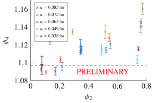
Figure 1: Measurements for $\phi_{4}$ show the mistuning in $\phi_{4}=\text{const}$. The physical point, as calculated by this analysis, is shown as a triangle.

To get the observables at a given value of $\phi_{4}$, we measured the derivatives $\frac{dX}{dm_{i}}$ of the observables $X$ with respect to the quark masses of all the involved measurements. With these we can construct the derivatives with respect to $\phi_{4}$,

$$\frac{dX}{d\phi_{4}}=\sum_{i=1}^{3}n_{i}\frac{dX}{dm_{i}}/\left(\sum_{i=1}^{3}n_{i}\frac{d\phi_{4}}{dm_{i}}\right).$$ (3)

Here $\vec{n}$ is the direction of the shift in the space of quark masses. It has an effect on distance of the shift needed to reach the given value of $\phi_{4}$ and thus on the resulting uncertainty. For the symmetric ensembles we use $\vec{n}=(1,1,1)/\sqrt{3}$ to preserve the symmetry and which was also the choice in [3]. For other ensembles, however, we use the direction $\vec{n}=(0,0,1)$, which we found to be close to optimal, in the sense that it minimizes the errors of the shifted values of $f_{\pi K}$. Since the shifts are typically less than $5\%$ in the sum of the quark masses, we do expect the leading order of the Taylor expansion to give results with a systematic error below our statistical uncertainty. This also has been verified with a few ensembles at the symmetric line at a different sum of quark masses.

In the 2016 analysis [3], we shifted the results on each ensemble individually. In our update, we now model the mass derivatives of the observables as a function of quark mass and lattice spacing. This makes the predictions more stable and also allows the use of ensembles, where the derivatives have not been measured. With these derivatives the measurements can now be shifted to the desired $\phi_{4}$ by

$$X(\phi_{4}^{\text{phys}})=X(\phi_{4})+\frac{dX}{d\phi_{4}}\left(\phi_{4}^{\text{phys}}-\phi_{4}\right).$$ (4)

3 Chiral and Continuum Extrapolation

In the description of the analysis, we now have data at any given value of $\phi_{4}$, which is a proxy for the sum of the two degenerate light and strange quark masses. To get to the physical point, we need to describe its chiral behavior and extrapolate to physical light quark masses given by $\phi_{2}^{\text{phys}}$.

Chiral perturbation theory [15, 16] predicts

$$f_{\pi K} =f\left[1-\frac{7}{6}L\left(\frac{\phi_{2}}{\bar{F}^{2}}\right)-\frac{4}{3}L\left(\frac{\phi_{4}-\frac{1}{2}\phi_{2}}{\bar{F}^{2}}\right)-\frac{1}{2}L\left(\frac{\frac{4}{3}\phi_{4}-\phi_{2}}{\bar{F}^{2}}\right)+k\phi_{4}+\mathcal{O}\left(M^{2}\right)\right]$$ (5)

for the quark mass dependence of $f_{\pi K}$ in terms of a single SU(3) $\chi$PT NLO low energy constant, $k\propto(L_{5}+3L_{4})$ as well as

$$L(x)=x\log(x)\,,\quad\bar{F}=4\pi\sqrt{8t_{0}}\,f.$$ (6)

We defined $\bar{F}$ in terms of $f$, the decay constant in the chiral limit. We then use a fit function for the chiral and continuum behavior

$$F_{\chi}(\phi_{2},\phi_{4}) =F_{\chi}^{\text{cont}}(\phi_{2},\phi_{4})\cdot\left(1+C\cdot\frac{a^{2}}{t_{0}}\right)$$ (7)

$$F_{\chi}^{\text{cont}}(\phi_{2},\phi_{4}) =\frac{A}{8\pi\sqrt{2}}\left[1-\frac{7}{6}L\left(\frac{\phi_{2}}{A^{2}}\right)-\frac{4}{3}L\left(\frac{\phi_{4}-\frac{1}{2}\phi_{2}}{A^{2}}\right)-\frac{1}{2}L\left(\frac{\frac{4}{3}\phi_{4}-\phi_{2}}{A^{2}}\right)+B\phi_{4}\right]$$ (8)

with the parameters $A=A(\phi_{4})$ and $B=B(\phi_{4})$ for each fixed value of $\phi_{4}$.

It is worthwhile to consider the ratio of the chiral function

$$\frac{F_{\chi}^{\text{cont}}(\phi_{2},\phi_{4})}{F_{\chi}^{\text{cont}}(\phi_{2}^{\text{sym}},\phi_{4})}=R_{\chi}(\phi_{2},\phi_{4})+\mathrm{O}(M^{2})$$ (9)

since

$$\begin{split}R_{\chi}(\phi_{2},\phi_{4})=1&-\frac{7}{6}L\left(\frac{\phi_{2}}{A^{2}}\right)-\frac{4}{3}L\left(\frac{\phi_{4}-\frac{1}{2}\phi_{2}}{A^{2}}\right)-\frac{1}{2}L\left(\frac{\frac{4}{3}\phi_{4}-\phi_{2}}{A^{2}}\right)\\ &+\frac{7}{6}L\left(\frac{\phi_{2}^{\text{sym}}}{A^{2}}\right)+\frac{4}{3}L\left(\frac{\phi_{4}-\frac{1}{2}\phi_{2}^{\text{sym}}}{A^{2}}\right)+\frac{1}{2}L\left(\frac{\frac{4}{3}\phi_{4}-\phi_{2}^{\text{sym}}}{A^{2}}\right)\end{split}$$ (10)

is free of parameters in NLO $\chi$PT, except for a weak dependence on $A$ in the logarithms. We observe no systematic deviations from NLO $\chi$PT as shown in fig. 2.

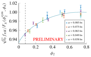
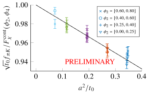
Figure 2: The chiral extrapolation on the left shows the measured data of $\sqrt{t_{0}}f_{\pi K}$ normalized by the fit function at the symmetric point. The solid line is the NLO $\chi$PT prediction, which does not depend on any NLO parameters and only logarithmically on the LO parameter $A$. No systematic deviation from this continuum formula can be detected. On the right, the continuum extrapolation of the same data, normalized by the fit-function evaluated for $a=0$, is shown.

In the same spirit the discretization effects are illustrated in the right hand plot of the same figure. Dividing each data point by the continuum $\chi$PT formula eq. 8 we expect the ratio

$$R_{\text{cont}}=\frac{F_{\chi}(\phi_{2},\phi_{4})}{F^{\text{cont}}_{\chi}(\phi_{2},\phi_{4})}=1+C\cdot\frac{a^{2}}{t_{0}}$$ (11)

to be a linear function in $a^{2}$ to leading order of the Symanzik expansion. Again, no deviation due to higher order terms is detected.

These considerations confirm the fit function given in eq. 7, from which we extract the central value and statistical uncertainty of $\sqrt{t_{0}}f_{\pi K}$. This central fit is displayed in fig. 3. It takes into account the data of the ensembles with $a<0.085\,\text{fm}$. The stability when applying other cuts to the data is considered later.

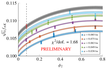
Figure 3: Chiral and Continuum Extrapolation of $\sqrt{t_{0}}f_{\pi K}$.

The combined chiral and continuum extrapolation is now evaluated at $\phi_{2}^{\text{phys}}$ to determine $\sqrt{t_{0}}f_{\pi K}$ at the physical point. Together with the values [19, 20]

$$f_{\pi}^{\text{isoQCD}}=130.56(02)(13)(02)\,\text{MeV},\quad f_{K}^{\text{isoQCD}}=157.2(2)(2)(4)\,\text{MeV}$$ (12)

in isospin symmetric pure QCD we are able to extract

$$\sqrt{t_{0}^{\text{phys}}}=\frac{\sqrt{t_{0}}f_{\pi K}}{f_{\pi K}^{\text{isoQCD}}}=0.1443(7)\,\text{fm}\quad\left(\chi\mathrm{PT\ fit},a<0.08\,\text{fm}\right)$$ (13)

from the $\chi$PT fit. The isoQCD values in eq. 12 are obtained from the experimental decay rates of $\pi\to\ell\nu+\gamma$ and $K\to\ell\nu+\gamma$ by taking out the QED and isospin effects with the help of $\chi$PT . This introduces the largest (second) error, while the first error is due to the experimental decay rate, and the third is due to the uncertainty of the CKM matrix elements $V_{ud}$ and $V_{us}$.

The physical scale $t_{0}^{\text{phys}}$ enters in the beginning of the analysis to define the physical point $\left(\phi_{2}^{\text{phys}},\phi_{4}^{\text{phys}}\right)$. We therefore find the fixpoint such that the resulting $t_{0}^{\text{phys}}$ is the same one that is used in the definition of the physical $\phi_{2}$ and $\phi_{4}$. For the statistical error of this final result the full correlation of the errors between the various observables is taken into account. We find the physical point at

$$\phi_{2}^{\text{phys}}=0.0779(7),\quad\phi_{4}^{\text{phys}}=1.098(10).$$ (14)

The fact that we do not observe significant deviations from the fit formula does, of course, not mean that they are not present. To estimate this source of systematic error, we use a range of different extrapolations: the $\chi$PT formula has been substituted by a Taylor expansion in the quark masses around the symmetric point and we also augmented the continuum extrapolation by an $a^{2}m_{\pi}^{2}$ term. Applying a series of cuts to the data by removing the coarsest lattices or the ones with larger pion masses, leads also to valid description of the data. All fits which we consider render a $\chi^{2}/\mathrm{dof}$ between $1$ and $2$. Fits where the probability to find a $\chi^{2}$ greater than the measured one is less than $5\%$ are discarded. We then take the minimum and the maximum central values and use half their difference as our preliminary systematic error and arrive at

$$\sqrt{t_{0}^{\text{phys}}}=0.1443(7)(13)\,\text{fm}.$$ (15)

At present, the systematic error dominates.

4 Lattice Spacing

Having determined the intermediate scale $t_{0}^{\text{phys}}$ at the physical point, we use it together with measurements for $t_{0}/a^{2}$ to calculate the lattice spacing $a$ in physical units. Since measurements at the physical point are not available for all lattice spacings, we need to model the behavior of $t_{0}$ as a function of $\phi_{2}$. Using next-to-leading order $\chi$PT [16] we arrive at the fit formula

$$R_{t_{0}}(\phi_{2})=\frac{\sqrt{t_{0}}}{\sqrt{t_{0}^{\text{sym}}}}=\sqrt{1+G\left(\phi_{2}-\phi_{2}^{\text{sym}}\right)}.$$ (16)

The data along with the fit are shown in fig. 5. We see quite clearly that at $a=0.085\,\text{fm}$ there are lattice artifacts which then disappear very quickly (more quickly than $a^{2}$). This phenomenon was also observed in fit 4. of Ref. [3]. We therefore perform a fit to the normalized scale $\sqrt{t_{0}/t_{0}^{\text{sym}}}$ leaving out the coarsest ensembles with $a=0.085\,\text{fm}$, as we have already done above. The figure is also good evidence for the smallness of mass-dependent $a^{2}$ effects. Further evidence is that the coefficients of mass-dependent cutoff effects in the Symanzik effective theory are very small for our discretization [17].

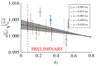
Figure 4: Scale $\sqrt{t_{0}}$ as a function of $\phi_{2}$ normalized by the scale at the symmetric point for each lattice spacing. The fit includes all but the coarsest ensemble with $a=0.085\,\text{fm}$.

$\beta$	$a\,\mathrm{[fm]}$
3.40	0.0849(5)(8)
3.46	0.0749(4)(7)
3.55	0.0633(4)(6)
3.70	0.0491(3)(4)
3.85	0.0385(2)(3)

Figure 5: Lattice spacings $a$ for each inverse coupling $\beta$ with statistic and systematic errors.

The ratio $R_{t_{0}}(\phi_{2}^{\text{phys}})$ allows us to determine the scale $t_{0}$ in physical units at the symmetric point, $\sqrt{t_{0}^{\text{phys}}}$ where we can use the measured values for $t_{0}/a^{2}$ to extract the lattice spacing,

$$a=\frac{\sqrt{t_{0}^{\text{phys}}}}{R_{t_{0}}(\phi_{2}^{\text{phys}})}\cdot\frac{1}{\sqrt{t_{0}^{\text{sym}}/a^{2}}}.$$ (17)

Using eq. 15 we arrive at the lattice spacings listed in fig. 5.

5 Conclusion and Outlook

The scale setting method presented here is one of many choices. Using the pseudo-scalar decay constants has the advantage that they can be easily and precisely calculated on the lattice. Contaminations by excited state contributions can be thoroughly controlled. On the other hand our method is limited by the necessity to relate the experimental decay rates which include photons in the final state to the pure QCD decay constants as well as the dependency on the CKM matrix element $V_{us}$. The latter means in particular that the validity of the Standard model at low energies is assumed. However, the estimated uncertainties due to QED and the CKM matrix elements are still significantly below our overall precision and we are able to improve the result from the 2016 analysis [3].

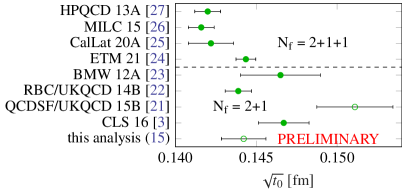
Figure 6: Comparison of $\sqrt{t_{0}}$ for different groups. Open symbols data points are not published.

Figure 6 compares the results from this analysis to previous determinations of $\sqrt{t_{0}}$ for $N_{f}=2+1$ flavor and $N_{f}=2+1+1$ flavor ensembles. It is worth noting that the central value of the previous CLS determination (labeled CLS 16) is more than $1\sigma$ above the current result. With the addition of several ensembles close to the physical point, it can now be seen that the point closest to the physical line in 2016 (purple point for $a=0.063\,\text{fm}$ at $\phi_{2}\approx 0.17$ in fig. 3) has a high statistical fluctuation upwards. This resulted in the previous analysis being skewed. It also highlights that precision scale setting, which is essential to precision results from lattice QCD, is a challenging endeavor. We need large statistics such that autocorrelations are under control as well as data at a large range of lattice spacings close to the continuum and quark masses sufficiently close to their physical values. Going significantly beyond the present accuracy will also require an improved control of isospin breaking and QED effects.

Acknowledgments.

S. Collins and R. Sommer were supported by the European Union’s Horizon 2020 research and innovation programme under the Marie Skłodowska-Curie grant agreement nos. 813942 (ITN EuroPLEx) and 824093 (STRONG- 2020). We thank our colleagues in the Coordinated Lattice Simulations (CLS) effort [http://wiki-zeuthen.desy.de/CLS/CLS] for the joint generation of the gauge field ensembles on which the computation described here is based.

We acknowledge PRACE for awarding us access to resource FERMI based in Italy at CINECA, Bologna and to resource SuperMUC based in Germany at LRZ, Munich. We acknowledge the Gauss Centre for Supercomputing e.V. (www.gauss-centre.eu) for providing computing time through the John von Neumann Institute for Computing (NIC) on JUQUEEN at Jülich Supercomputing Centre and on SuperMUC-NG at Leibniz Supercomputing Centre (www.lrz.de). We thank DESY for computing resources on the PAX cluster in Zeuthen.

References

- [1] M. Bruno et al., Simulation of QCD with N 2 1 flavors of non-perturbatively improved Wilson fermions, JHEP 02 (2015) 043 [1411.3982].
- [2] D. Mohler, S. Schaefer and J. Simeth, CLS 2+1 flavor simulations at physical light- and strange-quark masses, EPJ Web Conf. 175 (2018) 02010 [1712.04884].
- [3] M. Bruno, T. Korzec and S. Schaefer, Setting the scale for the CLS flavor ensembles, Phys. Rev. D 95 (2017) 074504 [1608.08900].
- [4] M. Lüscher, Properties and uses of the Wilson flow in lattice QCD, JHEP 08 (2010) 071 [1006.4518].
- [5] ALPHA collaboration, QCD Coupling from a Nonperturbative Determination of the Three-Flavor Parameter, Phys. Rev. Lett. 119 (2017) 102001 [1706.03821].
- [6] RQCD collaboration, Masses and decay constants of the and ’ mesons from lattice QCD, JHEP 08 (2021) 137 [2106.05398].
- [7] RQCD collaboration, Light-cone distribution amplitudes of octet baryons from lattice QCD, Eur. Phys. J. A 55 (2019) 116 [1903.12590].
- [8] RQCD collaboration, Light-cone distribution amplitudes of pseudoscalar mesons from lattice QCD, JHEP 08 (2019) 065 [1903.08038].
- [9] RQCD collaboration, Nucleon axial structure from lattice QCD, JHEP 05 (2020) 126 [1911.13150].
- [10] D. Djukanovic, T. Harris, G. von Hippel, P.M. Junnarkar, H.B. Meyer, D. Mohler et al., Isovector electromagnetic form factors of the nucleon from lattice QCD and the proton radius puzzle, Phys. Rev. D 103 (2021) 094522 [2102.07460].
- [11] A. Gérardin, M. Cè, G. von Hippel, B. Hörz, H.B. Meyer, D. Mohler et al., The leading hadronic contribution to from lattice QCD with flavours of O() improved Wilson quarks, Phys. Rev. D 100 (2019) 014510 [1904.03120].
- [12] D. Mohler and S. Schaefer, Remarks on strange-quark simulations with Wilson fermions, Phys. Rev. D 102 (2020) 074506 [2003.13359].
- [13] A. Ramos and S. Sint, Symanzik improvement of the gradient flow in lattice gauge theories, Eur. Phys. J. C 76 (2016) 15 [1508.05552].
- [14] J. Gasser and H. Leutwyler, Light Quarks at Low Temperatures, Phys. Lett. B 184 (1987) 83.
- [15] J. Gasser and H. Leutwyler, Chiral Perturbation Theory: Expansions in the Mass of the Strange Quark, Nucl. Phys. B 250 (1985) 465.
- [16] O. Bar and M. Golterman, Chiral perturbation theory for gradient flow observables, Phys. Rev. D 89 (2014) 034505 [1312.4999].
- [17] N. Husung, P. Marquard and R. Sommer, The asymptotic approach to the continuum of lattice QCD spectral observables, 2111.02347.
- [18] N. Husung, Asymptotic behavior of cutoff effects of Gradient Flow observables in lattice Yang-Mills theory, in preparation .
- [19] Y. Aoki et al., FLAG Review 2021, 2111.09849.
- [20] Particle Data Group collaboration, Review of Particle Physics, PTEP 2020 (2020) 083C01.
- [21] V.G. Bornyakov et al., Wilson flow and scale setting from lattice QCD, 1508.05916.
- [22] RBC, UKQCD collaboration, Domain wall QCD with physical quark masses, Phys. Rev. D 93 (2016) 074505 [1411.7017].
- [23] S. Borsanyi et al., High-precision scale setting in lattice QCD, JHEP 09 (2012) 010 [1203.4469].
- [24] Extended Twisted Mass collaboration, Ratio of kaon and pion leptonic decay constants with Nf=2+1+1 Wilson-clover twisted-mass fermions, Phys. Rev. D 104 (2021) 074520 [2104.06747].
- [25] N. Miller et al., Scale setting the Möbius domain wall fermion on gradient-flowed HISQ action using the omega baryon mass and the gradient-flow scales and , Phys. Rev. D 103 (2021) 054511 [2011.12166].
- [26] MILC collaboration, Gradient flow and scale setting on MILC HISQ ensembles, Phys. Rev. D 93 (2016) 094510 [1503.02769].
- [27] R.J. Dowdall, C.T.H. Davies, G.P. Lepage and C. McNeile, from and decay constants in full lattice QCD with physical , , and quarks, Phys. Rev. D 88 (2013) 074504 [1303.1670].