∎
Construction of Continuous Magnetic Cooling Apparatus with Zinc Soldered PrNi5 Nuclear Stages
Abstract
We report design details of the whole assembly of a compact and continuous nuclear demagnetization refrigerator (CNDR) with two PrNi5 nuclear stages, which can keep temperature below 1 mK continuously, and test results of a new thermal contact method for the PrNi5 stage using Zn soldering rather than Cd soldering. By measuring a residual electrical resistance of a short test piece, the thermal contact resistivity between the PrNi5 rod and an Ag wires thermal link was estimated as . Based on this value and 2D numerical and 1D analytical thermal simulations, the largest possible temperature gradient throughout the nuclear stage was calculated to be negligibly small ( 2 %) at 1 mK under a 10 nW heat leak, the expected cooling power of the CNDR.
Keywords:
nuclear demagnetization refrigerator PrNi5 contact resistance1 Introduction
Recently, a sub-mK temperature environment is recognized as one of the frontiers in research fields of material science Ref: Clark , nanoelectronics Ref: Palma , and cryogenic particle detector Ref: Shirron . The nuclear demagnetization refrigerator (NDR) with copper nuclear stage is a standard equipment to achieve such extremely low temperatures Ref: Pobell . However, construction and operation of NDRs are technically demanding, which has been preventing non-experts from making use of the sub-mK environment. In order to overcome the limitations, we recently proposed the concept of continuous refrigeration using two PrNi5 nuclear demagnetization stages and a dilution refrigerator connected in series each other via two superconducting heat switches Ref: Toda_1 . The numerical simulations under realistic conditions showed that this new type of refrigerator, the continuous nuclear demagnetization refrigerator (CNDR), can keep the sample temperature at 0.8 mK with a cooling power of 10 nW Ref: Toda_1 . Developments of CNDR are now actively conducted Ref: Schmoranzer_1 ; Ref: Takimoto ; Ref: Schmoranzer_2 .
In this article, after showing an updated total design of our CNDR in Sec. 2, we report construction details of the PrNi5 nuclear stage, one of major parts of the CNDR (Sec. 3). We tested a new soldering method with Zn for PrNi5 and estimated a thermal contact resistivity of the Zn contact between a PrNi5 rod and Ag wires from electrical resistance measurements (Sec. 4). Then, using known resistivities of all parts, a possible temperature gradient through the PrNi5 nuclear stage was evaluated from numerical and analytical calculations on thermal models (Sec. 5).
2 Practical Design of the CNDR
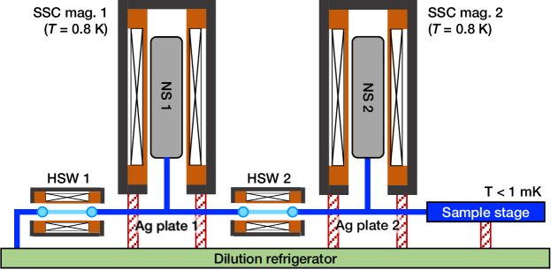
Figure 1 shows a schematic diagram of our CNDR. The CNDR consists of four major parts, (1) a standard dilution refrigerator which has a cooling power of at least 100 W at 100 mK, (2) two PrNi5 nuclear stages, (3) two shielded superconducting (SSC) magnets Ref: Takimoto and (4) two superconducting Zn heat switches. The PrNi5 stages are connected in series between the sample stage and the mixing chamber of the dilution refrigerator through the two heat switches. The CNDR can keep temperature below 1 mK continuously with a cooling power of 10 nW if the total thermal resistance among the four components is less than the value corresponding to a few hundreds n in the electrical resistance unit Ref: Toda_1 .
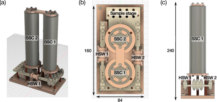
Figure 2 shows a three-dimensional CAD image of our latest version of CNDR. The nuclear stages and other components are assembled on a Cu base plate which is connected directly to the mixing chamber. The two SSC magnets are thermally anchored to the still of the dilution refrigerator and mechanically supported by Vespel SP-22 thermal insulation rods from the base plate. Three of four Ag thermal links for the heat switches and six Ag thermal links for the nuclear stages are tightly connected to two Ag plates of 5 mm thick with M4 Si0.15Ag0.85 (Tokuriki Honten Co., Ltd.) screws so as to be demountable. The cross section of each Ag thermal link is mm2. The contact areas of these parts are gold-plated of 3–4 m thickness to reduce the contact thermal resistance Ref: Okamoto . The maximum dimensions of the whole assembly of this CNDR are 160 mm in length, 84 mm in width and 240 mm in height, which are compact enough to be installable in most of dilution refrigerators.
3 Zinc Soldering of PrNi5 Nuclear Stage
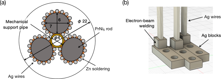
It is important to achieve a better thermal contact between a nuclear coolant and a thermal link to minimize a temperature gradient between them under finite heat flows. Figure 3 (a) shows a cross section of the PrNi5 nuclear stage of the CNDR. Each stage consisting of three PrNi5 rods of about 6 mm diameter and 120 mm long is soldered to the thermal link made of 15 Ag wires of 1 mm diameter with Zn as described in more detail later. It is noted that we cannot apply common press contact here because PrNi5 is so brittle and can easily crack under stress. The other ends of the Ag wires are electron-beam (EB) welded to the silver block (see Fig. 3 (b)). The depth and lateral dimensions of the welded part are 6 mm and 86 mm2, respectively. After the EB welding, the assembled Ag thermal link was annealed at for 3 hours in an O2 flow ( Pa). The residual resistivity ratio (RRR) of the Ag wire was increased from 300 to 2,300 by this heat treatment. From the four-wire measurement at 4.2 K, we determined a residual electrical resistance of the EB welded part to be n. This is lower than resistances of other parts throughout the nuclear stage (see later discussions). RRR of the PrNi5 rod is 42.
There are three common soldering agents to attach the PrNi5 rod to the thermal link, that are Cd Ref: Mueller ; Ref: Andres ; Ref: Greywall ; Ref: Parpia , In Ref: Wiegers and Sn Ref: Ishimoto_1 . Cd has most commonly been used in the previous works because of its low superconducting critical field ( mT). Note that limits the final field of demagnetization cooling. However, the problem of Cd is that it is toxic. In has a ten times higher than that of Cd and is mechanically rather weak. Sn has also a high , and sometimes the cold brittleness due to structural transformation Ref: Cohen causes trouble. In this work, as a substitute soldering agent for Cd, we tested to use Zn which has a low enough ( mT) and low health damage. A drawback of Zn is a little higher melting temperature (420 ∘C) (see Table 1).
|
|
|
Flux | Note | |||||||
|---|---|---|---|---|---|---|---|---|---|---|---|
| Cd | 321 | 0.56 | 3.0 | ZnCl2 or NH4Cl | toxic | ||||||
| In | 157 | 3.40 | 29.3 | high , soft | |||||||
| Sn | 232 | 3.75 | 30.9 | high , brittle | |||||||
| Zn | 420 | 0.85 | 5.3 | ZnCl2 + NH4Cl | high |
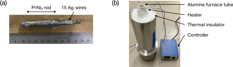
We evaluated the performance of the Zn soldering for the PrNi5 rod and Ag wires by making a short test piece shown in Fig. 4(a). Figure 4(b) shows a home-made furnace used in this test where a heater wire is wound around a high-purity (99.6 %) alumina furnace tube of 24 mm in inner diameter and 500 mm in height with a closed bottom. The alumina tube, in which molten Zn is filled, are thermally insulated by a rock wool. The tube temperature was kept around 480 ∘C with a PID controller during the soldering. The test piece was first immersed in a 10 wt% water solution of NaOH kept at 80 ∘C for 5 minutes for degreasing. After washing it with water, it was immersed in a 10 wt% water solution of HCl kept at 30 ∘C for 5 minutes for removing surface oxides. After washing it with water, it was then immersed in a flux, a 25 wt% water solution of a mixture of ZnCl2 (56 wt%) and NH4Cl (44 wt%), kept at 60 ∘C, and finally dipped in the molten Zn for 2 minutes for soldering.
4 Measurement of the Zn Soldered PrNi5/Ag Contact Resistance
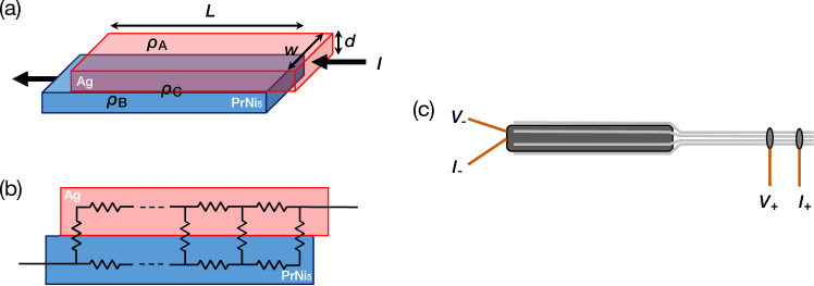
The thermal contact resistivity of the Zn-soldered Ag and PrNi5 contact was evaluated from a measurement of the total resistance of the test piece in the configuration shown in Fig. 5(a). The red and blue pieces here correspond to the Ag wires (A) and the PrNi5 rod (B), respectively. The contact area between A and B is denoted as C. The total resistance of this configuration is analytically given as the following equation Ref: Ishimoto_2 based on the ladder model shown in Fig. 5(b):
| (1) |
where
| (2) |
Here, and are volume resistivities of A and B, respectively, and is a contact resistivity. and are the length and the width of the contact area, respectively, and is the thickness of each piece. Since the ladder model is applicable to both thermal (t) and electrical (e) flow problems, superscripts t or e will be put on variables when we want to specify either t- or e-resistance in the following.
We measured of the test piece at 4.2 K in liquid 4He by using the four-terminal method shown in Fig. 5(c). and were determined from independent measurements for each Ag and PrNi5 pieces at 4.2 K. By substituting these values to eq.(1), we have . Since conduction electrons are carriers of both electrical and thermal flows in pure metals and metallic compounds at millikelvin temperatures, one can convert to assuming the Wiedemann-Franz law with the Lorenz number ( WK-2). The fairly good applicability of this law to PrNi5 is verified down to 100 mK Ref: Meijer . Then, we have the thermal contact resistivity as .
The obtained electrical resistivity of the Zn soldered PrNi5/Ag contact, which gives a total contact resistance of 4 n for each PrNi5 rod, is sufficiently low for our purpose. This can easily be understood if compared with the total electrical resistance of 140 n throughout the whole PrNi5 stage in Greywall’s single-stage nuclear demagnetization refrigerator Ref: Greywall . In the next section, we will confirm this more quantitatively.
5 Simulations for Temperature Gradient in the Nuclear Stage
Using the , and values obtained in the previous section, one can evaluate a temperature difference () throughout the nuclear stage under a given heat flow. In order to estimate the largest possible , we made numerical simulations based on the finite element method under a constrain that the temperature () along the central () axis of the PrNi5 rod is always kept at 1 mK as shown in Fig. 6(a) left. The constrain is equivalent to neglecting cooling powers associated with slow demagnetization of nuclear spins in off-axial segments within the PrNi5 rod. This intentionally increases a radial () temperature gradient than the actual situation. For simplicity, we also applied axisymmetry about the central axis to the model. This means that no azimuthal component of heat flow is considered. A constant heat flow of nW, which is one third of the expected total cooling power of our CNDR, was introduced from the top end of the Ag wires (see Fig. 6(a) left). Thus the temperature at that end is . The simulations were carried out using an open source software (FEMM: Finite Element Method Magnetics by David Meeker). In the simulation, a – (two dimensional: 2D) plane of the nuclear stage is divided to 16,000 elements.
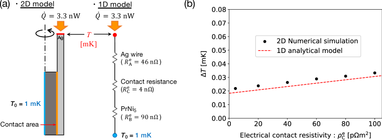
Results of the simulation for six different ( p) are shown as the dots in Fig. 6(b). For the value () we obtained with the Zn soldering, is expected to be less than 20 K at mK, which is negligibly small. is not sensitive to and will not exceed 10% unless becomes larger by two orders of magnitude.
The dashed line in Fig. 6(b) is an expected behavior from the one-dimensional (1D) model considering serially connected three thermal resistances which are the resistance of the Ag wires () above the stage, that of the PrNi5 () and the contact resistance () between them (see Fig. 6(a) right). and are calculated from and neglecting the resistance of the Ag wires over the length of the PrNi5 rod and considering only the component of heat flow. This simplification resembles to the constraint of fixed (= 1 mK) along the axis in the 2D numerical simulation described above. The analytical solution of the 1D model is expressed as:
| (3) |
where m, m, and m are geometrical factors. As can be seen in Fig. 6(b), the 1D analytical model gives slightly smaller values than the 2D numerical simulation, because the temperature variation along the direction is neglected. However, the difference (8–16 %) is small and the 1D model is much simpler to calculate, so it is a more convenient estimator of .
6 Conclusion
We described design details of the whole assembly of the continuous nuclear demagnetization refrigerator (CNDR) which is so compact that it can be installed on the mixing chamber of an existing dilution refrigerator. We focused on the design of the PrNi5 nuclear stage, a central part of the CNDR, in this article. As an alternative to the widely-used Cd soldering thermal contact for PrNi5, the Zn soldering was proposed and tested. From the residual electrical resistance measurements of a short test piece, the thermal contact resistivity between the PrNi5 rod and the Ag wires was estimated as assuming the Wiedemann-Franz law. This is favorably compared with the previously reported contact resistivities for other metals and soldering agents. Using known resistivities of all major parts of the CNDR, we evaluated the largest possible temperature gradient throughout the nuclear stage from the 2D numerical and 1D analytical calculations. The calculations show a negligibly small (%) at 1 mK under a 10 nW heat leak, which is an expected cooling power of the CNDR. All parts of the CNDR are now being assembled anticipating the first cooling test.
Acknowledgements.
We thank the machine shop of the School of Science, the University of Tokyo for machining most of the parts of CNDR. ST was supported by Japan Society for the Promotion of Science through Program for Leading Graduate Schools (MERIT).References
- (1) A. C. Clark, K. K. Schwarwalder, T. Bandi, D. Maradan, and D. M. Zumbuhl, Rev. Sci. Instrum. 81, 103904 (2010).
- (2) M. Palma, D. Maradan, L. Casparis, T.-M. Liu, F. N. M. Froning, and D. M. Zumbuhl, Rev. Sci. Instrum. 88, 043902 (2017).
- (3) P. Shirron, D. Wegel, M. DiPirro, and S. Sheldon, Nuclear Instruments and Methods in Physics Research A 559, 651 (2006).
- (4) F. Pobell, Matter and Methods at Low Temperatures, 3rd ed. (Springer, Berlin, 2007).
- (5) R. Toda, S. Murakawa, and H. Fukuyama, J. Phys.: Conf. Ser. 969, 012093 (2018).
- (6) D. Schmoranzer, R. Gazizulin, S. Triqueneaux, E. Collin, A. Fefferman, J. Low Temp. Phys. 196(1-2), 261 (2019).
- (7) S. Takimoto, R. Toda, S. Murakawa, and H. Fukuyama, J. Low Temp. Phys. 201, 179 (2020).
- (8) D. Schmoranzer, J. Butterworth, S. Triqueneaux, E. Collin, A. Fefferman, Cryogenics 110, 103119 (2020).
- (9) T. Okamoto, H. Fukuyama, H. Ishimoto, and S. Ogawa, Rev. Sci. Instrum. 61, 1332 (1990).
- (10) R. Mueller, C. Buchal, H. Folle, M. Kubota, and F. Pobell, Cryogenics 20(7), 395 (1980).
- (11) K. Andres and S. Darack, Physica B+C 86-88(PART 3), 1071 (1977).
- (12) D. Greywall, Phys. Rev. B 31, 2675 (1985).
- (13) J. Parpia, W. Kirk, P. Kobiela, T. Rhodes, Z. Olejniczak, and G. Parker, Rev. Sci. Instrum. 56, 437 (1985).
- (14) S. Wiegers, T. Hata, C. Kranenburg, P. van de Haar, R. Jochemsen, and G. Frossati, Cryogenics 30(9), 770 (1990).
- (15) H. Ishimoto, N. Nishida, T. Furubayashi, M. Shinohara, Y. Takano, Y. Miura, and K. Ono, J. Low Temp. Phys. 55(1-2), 17 (1984).
- (16) E. Cohen and A. K. W. A. van Lieshout, Z. Physik. Chem. 173, 32 (1935).
- (17) H. Ishimoto, H. Fukuyama, N. Nishida, Y. Miura, Y. Takano, T. Fukuda, T. Tazaki, and S. Ogawa, J. Low Temp. Phys. 77, 133 (1989).
- (18) H. C. Meijer, G. J. C. Bots, and H. Postma, Physica 107B, 607 (1981).