Multi-Modal Mutual Information Maximization:
A Novel Approach for Unsupervised Deep Cross-Modal Hashing

Abstract

In this paper, we adopt the maximizing mutual information (MI) approach to tackle the problem of unsupervised learning of binary hash codes for efficient cross-modal retrieval. We proposed a novel method, dubbed Cross-Modal Info-Max Hashing (CMIMH). First, to learn informative representations that can preserve both intra- and inter-modal similarities, we leverage the recent advances in estimating variational lower-bound of MI to maximizing the MI between the binary representations and input features and between binary representations of different modalities. By jointly maximizing these MIs under the assumption that the binary representations are modelled by multivariate Bernoulli distributions, we can learn binary representations, which can preserve both intra- and inter-modal similarities, effectively in a mini-batch manner with gradient descent. Furthermore, we find out that trying to minimize the modality gap by learning similar binary representations for the same instance from different modalities could result in less informative representations. Hence, balancing between reducing the modality gap and losing modality-private information is important for the cross-modal retrieval tasks. Quantitative evaluations on standard benchmark datasets demonstrate that the proposed method consistently outperforms other state-of-the-art cross-modal retrieval methods.

I Introduction

The last few years have witnessed an exponential surge in the amount of information available online in heterogeneous modalities, e.g., images, tags, text documents, videos, subtitles, etc. Thus, it is desirable to have a single efficient system that can facilitate large-scale multi-media searches. In general, this system should support both single and cross-modality searches, i.e., the system returns a set of semantically relevant results of all modalities given a query in any modality. In addition, to be used in large scale applications, the system should have efficient storage and fast searching. Several cross-modality hashing approaches have been proposed to handle the above challenges, in both supervised [1, 2, 3, 4, 5, 6, 7, 8, 9, 10, 11, 12, 13, 14, 15, 16, 17, 18, 19, 20, 21, 22] and unsupervised [23, 24, 25, 26, 27, 28, 29, 30, 31, 32, 33, 34, 35, 36, 37] manners. Furthermore, as the unsupervised hashing does not require any label information, it is suitable for large-scale retrieval problem in which the label information is mostly unavailable. Thus, in this work, we focus on the unsupervised setting of the cross-modality hashing problem for retrieval tasks.

When learning binary representations for the cross-modal retrieval task, it is essential to preserve both intra- and inter-modal similarities in a common Hamming space. Equivalently, the binary representations should satisfy several requirements: (i) First, the representations necessarily capture information from the input features, i.e., preserve intra-modal similarity. (ii) For the representations of a modality to effectively retrieve samples of other modalities (i.e., the inter-modal similarity is preserved), the representations of this modality should capture as much information about other modalities as possible. Additionally, (iii) the modality gap (i.e., heterogeneous gap) between the representations of different modalities should be minimized, i.e., binary codes of all modalities should be in the same common space and binary codes from different modalities of the same instance (which contain the same information) should be as similar as possible [38, 39, 29]. Minimizing the modality gap is necessary for the similarity between different modalities to be measured directly.

To preserve both intra- and inter-modal similarities in the unsupervised setting, many existing cross-modality hashing methods, both CNN-based and non CNN-based, relied on similarity matrices/graphs (one for each modality [23, 25, 40, 28, 39] or to a joint similarity matrix for all modalities [29]). Then they learn hash codes via the eigenvalue decomposition of the similarity matrices. However, constructing the similarity matrix could be challenging and computationally expensive for large datasets. Furthermore, eigenvalue decomposition decreases the mapping quality substantially when increasing the hash code length [41]. Matrix Factorizaton (MF) based methods could avoid the large scale graph constructing and eigen-decomposition process by finding a shared latent semantic space [26, 41] that can reconstruct input data well for all modalities. However, only simple and capability-limited linear projection is used in MF-based methods. In addition, scaling up MF-based methods for much larger datasets is non-trivial. Recently, Li et. al. proposed Unsupervised coupled Cycle generative adversarial Hashing networks (UCH) [42], which used pair-coupled generative adversarial networks (GAN) to learn representations for individual modality and generate compact hash codes. Even though, this approach can achieve very competitive performance, training the minimax loss of GAN can be challenging.

Taking a different approach, inspired by recent advances in unsupervised representation learning [43, 44, 45, 46]; in this paper, we propose to learn informative binary representations for unsupervised cross-modal hashing via maximizing mutual information (MI). We learn to preserve the intra-modal and inter-modal similarities via maximizing the MI between representations and input and the MI between representations of different modalities. More specifically, by adopting the Variational Information Maximization method [47], we can use the binary representations to be modeled by multivariate Bernoulli distributions. As a result, the binary representations can be learned easily and effectively by maximizing the MI between themselves and input via maximizing the estimated variational MI lower-bounds [47, 48, 49, 50, 51] using gradient descent optimization in the mini-batch manner.

Furthermore, we find out that trying to minimize modality gap by learning similar binary representations for the same instance from different modalities could result in undesirable side-effect. Specifically, the modality-private information (i.e., the information of one modality that does not share with any other modality) is discarded. Consequently, the representations may become less representative for the input. Hence, balancing between reducing modality gap and losing modality-private information is important for the cross-modal retrieval tasks.

In addition to the above requirements for cross-modal retrieval tasks, independence and balance are well-known to be important properties of informative hash codes [52, 53, 54, 55, 56, 57]. The independence property, i.e., different bits in the binary codes are independent to each other, is to ensure hash codes do not capture redundant information. The balance property, i.e., each bit has a $50\%$ chance of being $0$ or $1$, is to ensure hash codes contain a maximum amount of information [54]. By assuming the binary representations to be modeled by multivariate Bernoulli distributions, we propose to leverage the Total Correlation (TC) [58] as a regularizer (i.e., minimizing TC) to enhance the independence between hash bits. Furthermore, the balanced property can also be achieved by regularizing the Bernoulli distributions such that the averaged probabilities over a training set for a bit to be $0$ or $1$ are equal and equal to $50\%$.

In summary, by adopting the maximizing mutual information approach, we propose a novel framework, dubbed Cross-Modal Info-Max Hashing (CMIMH), whose main contributions are:

• We propose to adopt the maximizing MI approach to learn binary representations for the cross-modal retrieval tasks. Besides maximizing MI between the representations and inputs, we explicitly maximize the MI between representations of different modalities, which is important to learn informative representations for cross-modal retrieval tasks.

• We find out that minimizing modality gap by learning similar binary representations for the same instance from different modalities could result in less informative representations. Since both informative representations and modality gap are important for cross-modal retrieval tasks, properly balancing these two factors is important to achieve good performance, as shown in our experiments. To the best of our knowledge, our work is the first work that provide in-depth analyses about the trade-off between these two factors.

• We propose to leverage the Total Correlation (TC) as a regularizer to enhance the independence between hash bits. The experimental results confirm that minimizing TC results in more independence hash bits and higher performance.

• We compare our proposed method against various state-of-the-art unsupervised cross-modality hashing methods on three standard cross-modal benchmark datasets, i.e., MIR-Flickr25K, NUS-WIDE, and MS-COCO. Quantitative results justify our contributions and demonstrate that CMIMH outperforms the compared methods on various evaluation metrics and settings.

II Related works

In this section we briefly discuss noticeable methods proposed cross-modal hashing.

Supervised Cross-modal hashing. Supervised hashing methods can explore the semantic information to enhance the data correlation from different modalities (i.e., reduce modality gap) and reduce the semantic gap. Many supervised cross-modal hashing methods with shallow architectures have been proposed, for instance Co-Regularized Hashing (CRH) [1], Heterogeneous Translated Hashing (HTH) [2], Supervised Multi-Modal Hashing (SMH) [3], Quantized Correlation Hashing (QCH) [4], Semantics-Preserving Hashing (SePH) [5], Discrete Cross-modal Hashing (DCH) [6], and Supervised Matrix Factorization Hashing (SMFH) [8]. All of these methods are based on hand-crafted features, which cannot effectively capture heterogeneous correlation between different modalities and may therefore result in unsatisfactory performance. Unsurprisingly, recent deep learning-based works [11, 12, 13, 14, 59, 15, 16, 10] can capture heterogeneous cross-modal correlations more effectively. Deep cross-modal hashing (DCMH) [12] simultaneously conducts feature learning and hash code learning in a unified framework. Pairwise relationship-guided deep hashing (PRDH) [15], in addition, takes intra-modal and inter-modal constraints into consideration. Deep visual-semantic hashing (DVSH) [16] uses CNNs, long short-term memory (LSTM), and a deep visual semantic fusion network (unifying CNN and LSTM) for learning isomorphic hash codes in a joint embedding space. However, the text modality in DVSH is only limited to sequence texts (e.g., sentences). In Cross-Modal Deep Variational Hashing [14, 60], the authors first proposed to learn shared binary codes from a fusion network, then learn generative modality-specific networks for encoding out-of-sample inputs. In Cross-modal Hamming Hashing [61], the author proposed Exponential Focal Loss which puts higher losses on pairs of similar samples with Hamming distance much larger than 2 (in comparison with the sigmoid function with the inner product of binary codes). Mandal et al. [9] proposed Generalized Semantic Preserving Hashing (GSPH) which can work for unpaired inputs (i.e., given a sample in one modality, there is no paired sample in other modality.). Song et al. [18] took advantage of the memory mechanism to design a memory network that can learn to store supporting information and retrieve the necessary information in reference. Xie et al. [19] proposed Multi-Task Consistency-Preserving Adversarial Hashing (CPAH), which consists of two modules: consistency refined module to learn modality-common and modality-private representations and multi-task adversarial learning module to preserve the semantic consistency information between different modalities. Ji et. al. [62] proposed a attribute-guided network (AgNet) framework to narrow the semantic gap brought by modality heterogeneity and category migration for the zero-shot cross-modal retrieval.

Although supervised hashing typically achieves very high performance, it requires a labor-intensive process to obtain large-scale labels, especially for multi-modalities, in many real-world applications. In contrast, unsupervised hashing does not require any label information. Hence, it is suitable for large-scale image search in which the label information is usually unavailable.

Unsupervised Cross-modal hashing. Cross-view hashing (CVH) [23] and Inter-Media Hashing (IMH) [25] adopt Spectral Hashing [52] for the cross-modality hashing problem. These two methods, however, produce different sets of binary codes for different modalities, which may result in limited performance. Linear cross-modal hashing (LCMH) [40] reduces the training complexity of IMH by representing training data with some cluster centers to avoid the large-scale graph construction process. In Predictable Dual-View Hashing (PDH) [24], the authors introduced the predictability to explain the idea of learning linear hyper-planes that each one divides a particular space into two subspaces represented by $-1$ or $1$. The hyper-planes, in addition, are learned in a self-taught manner, i.e., to learn a certain hash bit of a sample by looking at the corresponding bit of its nearest neighbors. Collective Matrix Factorization Hashing (CMFH) [26] aims to find consistent hash codes from different views by collective matrix factorization. Latent Semantic Sparse Hashing (LSSH) [27] was proposed to learn hash codes in two steps: first, latent features from images and texts are jointly learned with sparse coding, and then hash codes are achieved by using matrix factorization. Subsequently, Wang et al. [41] proposed Robust and Flexible Discrete Hashing (RFDH) which directly optimizes and generates the unified binary codes for various views in the unsupervised manner via matrix factorization such that large quantization errors caused by relaxation can be relieved to some extent. Inspired by CCA-ITQ [53], Go et al. [28] proposed Alternating Co-Quantization (ACQ) to alternately minimize the binary quantization error for each of modalities. In [29], the authors applied Nearest Neighbor Similarity [63] to construct Fusion Anchor Graph (FSH) from text and image modals for learning binary codes. Recently, proposed Collective Affinity Learning Method (CALM) [35], which collectively and adaptively learns hashing functions in an unsupervised manner with an anchor graph constructed on partial multi-modal data. We would like to refer readers to [64] for a more comprehensive survey on non-DNN-based cross-modal retrieval methods.

In addition to the aforementioned shallow methods, several works [31, 32, 33] utilized (stacked) auto-encoders for learning binary codes. These methods try to minimize the distance between hidden spaces of modalities to the preserve inter-modal semantic to a certain extent. Deep Binary Reconstruction (DBRC) [65] proposed to minimize the reconstruction error based on the shared binary representation. DBRC additionally proposed a scalable $\tanh$ activation with a learnable parameter, which can mitigate the gradient problem of the discrete domain of $\{-1,1\}$ during training. Recently, Zhang et al. [66] propsoed Multi-pathway Generative Adversarial Hashing (MGAH), which consists of a generative model and a discriminative model. In which, the generative model fits the distribution over the manifold structure and selects informative data of other modalities. While the discriminative model learns to discriminate data generated from the generative model and data sampled a correlation graph (a graph which captures the underlying manifold structure across different modalities). Wu et al. [39] proposed Unsupervised Deep Cross Modal Hashing (UDCMH), that enables the feature learning to be jointly optimized with the binarization. Su et al. [38] proposed a joint-semantics affinity matrix, which integrates the neighborhood information of two modals, for mini-batch samples to train deep network in an end-to-end manner. Li et. al. proposed Unsupervised coupled Cycle generative adversarial Hashing networks (UCH) [42], which used pair-coupled generative adversarial networks to learn representations for individual modality and generate compact hash codes. Given a multi-modal unpaired data, Wu et al. [67] adopted the cycle-consistent loss [68] to learn hashing functions. Although these methods make great progresses, the performance of these systems still has room for improvement.

Representation learning with Mutual Information: In MIHash [69], the authors proposed to use mutual information (MI) to learn hash codes for online hashing. In specific, given two Hamming distance distributions of a sample with its neighbors and its non-neighbors, the MI is used to measure the separability of these two distributions, which gives a good quality indicator for online hashing. However, this method is only proposed for the single modality case in a supervised manner, while our proposed method aims to learn binary representations for cross-modal retrieval in an unsupervised manner. In [70], the authors only adopted MI to learn to preserve intra-modal similarity, while our proposed method utilized MI to preserve both intra-modal and inter-modal similarities. Additionally, in contrast with [70] which learns real-valued representations, our method learns binary representations for large-scale retrieval. Besides, several works [43, 71, 45, 46, 72, 73] rely on MI to learn representations in unsupervised/self-supervised manner for single view and/or multi-view settings. Specifically, Hjelm et. al. [43] proposed to learn a global image representation such that the MI between this global representation and local features are maximized. Bachman et. al. [45] further improved [43] by maximizing the MI between a global representation and local features of the different views (i.e., different images generated by data augmentation). Different from [43, 45], [74] adopted the Information Bottleneck (IB) objective [75] with a variational approximation to minimize the MI between the input and the representation, while still ensuring the global representations can fulfill the target task (e.g., classification). This learning method could result in more robust representations. In [46], with the assumption that any single view can fully contain information of labels of a down-stream task (e.g., classification), the authors aimed to learn robust representations by capturing the shared information between views and discarding the private information (i.e., information that is exclusively contained in a particular view). Information Competing Process (ICP) [71] is another intriguing MI-based representation learning method. ICP aims to learn diversified representations by first separating a representation into two parts with different MI constraints, and then forcing separated parts to accomplish the downstream task independently without any knowledge of what the other part has learned. However, these works [43, 71, 45, 46, 72, 73] mainly focus on learning a single real-valued representation from single/multi-view inputs for classification. In contrast, our work aims to learn binary representations for multi-modal retrieval.

III Proposed method

Given a multi-modality dataset of $N$ instances, denoted as $\mathcal{O}=\{\mathbf{o}_{j}\}_{j=1}^{N}$, in which each instance is described by an image-text pair $\mathbf{o}_{j}=(\mathbf{x}^{{i}}_{j},\mathbf{x}^{{t}}_{j})$, where $\mathbf{x}^{{i}}_{j}\in\mathbb{R}^{D^{i}}$ and $\mathbf{x}^{{t}}_{j}\in\mathbb{R}^{D^{t}}$ are the $j$-th $D^{i},D^{t}$ dimensional features of image and text modalities respectively. We aim to learn the corresponding $L$-bit binary representations $\mathbf{h}^{{i}}_{j}$ and $\mathbf{h}^{{t}}_{j}\in\{0,1\}^{L}$ for each image and text pair $(\mathbf{x}^{{i}}_{j},\mathbf{x}^{{t}}_{j})$.

For representations being suitable for the cross-modal retrieval task, the representations should satisfy several requirements: (i) First, the representations should well represent the input data, i.e., they necessarily capture information from the input features. (ii) Second, for the image representations to effectively retrieve text samples, the image representations should capture as much information about the text modality as possible. Analogously, the text representation should contain as much information about the image modality as possible to retrieve image samples effectively. (iii) Third, the representations of different modalities should be well aligned with each other (i.e., the modal gap is minimized).

III-A Mutual Information Maximization

Mutual information (MI) has been proven to be an important quantity in data science to measure the dependence of two random variables, since it can capture non-linear statistical dependencies between variables [50]. Recent representation learning methods [45, 43] showed that MI maximization between inputs and encoder outputs can help to learn informative representations. Hence to achieve the first requirement, we aim to maximize the MI between the binary representations and the input data. Noticeably, in the ideal case, when the representations fully capture all input information; the MI between image and text representations would be maximized and be equal to the MI between the image and text input data (which is a constant). Equivalently, the second requirement would be satisfied. However, in practice, the representations may not fully capture all input information. Hence, we propose to further enforce the second requirement by explicitly maximizing the MI between the representations of image and text modalities. Our initial objective now can be written as follows:

$$\max I(\mathbf{x}^{{i}};\mathbf{h}^{{i}})+I(\mathbf{x}^{{t}};\mathbf{h}^{{t}})+I(\mathbf{h}^{{i}};\mathbf{h}^{{t}}).$$ (1)

However, MI is well-known to be notoriously difficult to compute. To handle this trouble, we propose to assume the image and text representations to be random variables; so that we can leverage recent advances in estimating variational lower bounds of MI [47, 48, 49, 50, 51] to maximize the objective function (1).

III-B Variational Lower Bounds of MI

III-B1 Variational Information Maximization

Directly optimizing $I(\mathbf{x}^{{i}};\mathbf{h}^{{i}})$ and $I(\mathbf{x}^{{t}};\mathbf{h}^{{t}})$ in the objective (1) is infeasible as the true posterior distributions (i.e., $P(\mathbf{x}^{{i}}|\mathbf{h}^{{i}}),P(\mathbf{x}^{{t}}|\mathbf{h}^{{t}})$) requiring for computing the MI is still unknown. Fortunately, we can use the Variational Information Maximization [47, 48] to compute the MI lower bound, in which $Q_{\phi_{i}}(\mathbf{x}^{{i}}|\mathbf{h}^{{i}})$ can be used to approximate the true posterior distribution, as follows:

$$\begin{split}I(\mathbf{x}^{{i}};\mathbf{h}^{{i}})&=H(\mathbf{x}^{{i}})-H(\mathbf{x}^{{i}}|\mathbf{h}^{{i}})\\ &=H(\mathbf{x}^{{i}})+\mathbb{E}_{p(\mathbf{x}^{{i}})}\big{[}\mathbb{E}_{P_{\theta_{i}}(\mathbf{h}^{{i}}|\mathbf{x}^{{i}})}[\log{P(\mathbf{x}^{{i}}|\mathbf{h}^{{i}})}]\big{]}\\ &=H(\mathbf{x}^{{i}})+\mathbb{E}_{p(\mathbf{x}^{{i}})}\big{[}D_{\text{KL}}[P(\mathbf{x}^{{i}}|\mathbf{h}^{{i}})||Q_{\phi_{i}}(\mathbf{x}^{{i}}|\mathbf{h}^{{i}})]\\ &\qquad\qquad\qquad\qquad\quad+\mathbb{E}_{P_{\theta_{i}}(\mathbf{h}^{{i}}|\mathbf{x}^{{i}})}[\log{Q_{\phi_{i}}(\mathbf{x}^{{i}}|\mathbf{h}^{{i}})}]\big{]}\\ &\geq H(\mathbf{x}^{{i}})+\mathbb{E}_{p(\mathbf{x}^{{i}})}\big{[}\mathbb{E}_{P_{\theta_{i}}(\mathbf{h}^{{i}}|\mathbf{x}^{{i}})}[\log{Q_{\phi_{i}}(\mathbf{x}^{{i}}|\mathbf{h}^{{i}})}]\big{]},\end{split}$$ (2)

where $H(\cdot)$ is the entropy function of a random variable; $\mathbb{E}$ is expectation, and $\theta_{i};\phi_{i}$ represent the model parameters of the encoder and decoder distributions, respectively. Similarly, we have

$$I(\mathbf{x}^{{t}};\mathbf{h}^{{t}})\geq H(\mathbf{x}^{{t}})+\mathbb{E}_{p(\mathbf{x}^{{t}})}\big{[}\mathbb{E}_{P_{\theta_{t}}(\mathbf{h}^{{t}}|\mathbf{x}^{{t}})}[\log{Q_{\phi_{t}}(\mathbf{x}^{{t}}|\mathbf{h}^{{t}})}]\big{]}.$$ (3)

Note that $H(\mathbf{x}^{{i}})$ and $H(\mathbf{x}^{{t}})$ are constant for the given input data. To be concise, from now on, we skip the subscript about model parameters in the encoder and decoder distributions whenever the context is clear.

As we aim to obtain binary representations for the cross-modal hashing, we adopt the multivariate Bernoulli distributions to model the encoder distributions $P(\mathbf{h}^{{i}}|\mathbf{x}^{{i}})$ and $P(\mathbf{h}^{{t}}|\mathbf{x}^{{t}})$; i.e., $P(\mathbf{h}^{{i}}|\mathbf{x}^{{i}}):=\text{Bern}(\boldsymbol{\mu}^{i})$ and $P(\mathbf{h}^{{t}}|\mathbf{x}^{{t}}):=\text{Bern}(\boldsymbol{\mu}^{t})$. Additionally, we assume that the decoder distributions $Q(\mathbf{x}^{{i}}|\mathbf{h}^{{i}})$ and $Q(\mathbf{x}^{{t}}|\mathbf{h}^{{t}})$ are Gaussian. Therefore, the log likelihoods in (2) and (3) can be maximized by minimizing $L2$ reconstruction loss.

III-B2 Reparameterization trick

Following [76, 77], we can reparameterize $\mathbf{h}\sim\text{Bern}(\boldsymbol{\mu})$ as $\mathbf{h}=\mathrm{sign}(\mathbf{z})$ (i.e., $\mathrm{sign}(z)=1$ if $z\geq 0$ and $\mathrm{sign}(z)=0$ if $z<0$), where ${\boldsymbol{z}}$ is a vector of independent logistic random variables defined as follows

$$\mathbf{z}=g(\mathbf{u},\boldsymbol{\mu})=\log\frac{\boldsymbol{\mu}}{1-\boldsymbol{\mu}}+\log\frac{\mathbf{u}}{1-\mathbf{u}},$$ (4)

where $\mathbf{u}\sim\text{Uniform}(0,1)$. Even though this reparameterization trick can help to avoid sampling from the Bernoulli distribution, this trick still requires a discrete threshold function which hinders the gradient descent optimization. To handle this difficulty, we resort to the Straight-Through Estimator (STE) [78], i.e., $\frac{\partial\mathrm{sign}(z)}{\partial z}=1$, to approximate the gradients propagating through the $\mathrm{sign}$ function.

III-B3 Sample-based differentiable MI lower bound

Different from $I(\mathbf{x}^{{i}};\mathbf{h}^{{i}})$ and $I(\mathbf{x}^{{t}};\mathbf{h}^{{t}})$; in $I(\mathbf{h}^{{i}};\mathbf{h}^{{t}})$, we can access samples from two random variables independently. This allows us to maximize the MI between the two representations $I(\mathbf{h}^{{i}};\mathbf{h}^{{t}})$ using a sample-based differentiable MI lower bound, which could have a tighter bound than (2) and (3) in practice [79]. Furthermore, as our primary interest is to maximize the MI, and not to find its precise value; we can rely on non-KL divergences estimator, i.e., a Jensen-Shannon MI estimator ($I_{\text{JS}}$), which is observed to work better in practice (e.g., more stable) than the KL divergences MI estimator (e.g., Donsker-Varadhan representation (DV) [80] or $f$-divergences [49]) [43]. The sample-based differentiable Jensen-Shannon MI estimator ($I_{\text{JS}}$) could be defined as follows

$$I(\mathbf{h}^{{i}};\mathbf{h}^{{t}})\propto I_{\text{JS}} (\mathbf{h}^{{i}};\mathbf{h}^{{t}})=D_{\text{JS}}\left[p(\mathbf{h}^{{i}},\mathbf{h}^{{t}})\big{\|}p(\mathbf{h}^{{i}})p(\mathbf{h}^{{t}})\right]$$ (5)

$$\geq\sup_{T\in\mathcal{F}}\mathbb{E}_{p(\mathbf{h}^{{i}},\mathbf{h}^{{t}})}[\bar{T}]+\mathbb{E}_{p(\mathbf{h}^{{i}})p(\mathbf{h}^{{t}})}[\log(2-\exp(\bar{T}))],$$

where $\mathcal{F}$ is a family of functions $T(\boldsymbol{h}^{{i}};\boldsymbol{h}^{{t}})\in\mathbb{R}$, parameterized by neuron networks, which is jointly optimized during the training procedure to classify if a pair of samples are from the joint distribution $p(\mathbf{h}^{{i}},\mathbf{h}^{{t}})$ or the product of marginal distributions $p(\mathbf{h}^{{i}})p(\mathbf{h}^{{t}})$, i.e., pairs of $(\boldsymbol{h}^{{i}};\boldsymbol{h}^{{t}})$ are produced from the pairs of inputs sampled from joint distributions $p(\mathbf{x}^{{i}},\mathbf{x}^{{t}})$ or sampled from the product of marginal distributions $p(\mathbf{x}^{{i}})p(\mathbf{x}^{{t}})$, respectively [49, 50]. Additionally, $\bar{T}=\log(2)-\log(1+\exp(-T))$ [49].

From (5), we can see that if the function $T$ can correctly classify between samples from the joint and product of marginal distributions with high confident, the MI lower bound will be maximized. However, we found that the process of jointly training the function $T$ (with binary inputs sampled from $\boldsymbol{h}^{i}\sim\text{Bern}(\boldsymbol{\mu}^{i})$ and $\boldsymbol{h}^{t}\sim\text{Bern}(\boldsymbol{\mu}^{t})$) and the encoders may result in an undesirable side-effect. Particularly, besides encouraging the encoders to learn the hidden variables for different modalities, such that the MI of these hidden variables is maximized; the function $T$ also promotes the encoders to reduce the stochasticity in $\text{Bern}(\boldsymbol{\mu}^{i})$ and $\text{Bern}(\boldsymbol{\mu}^{t})$ (i.e., $\boldsymbol{\mu}\to 0$ or $\boldsymbol{\mu}\to 1$). Intuitively, reducing stochasticity in $\text{Bern}(\boldsymbol{\mu}^{i})$ and $\text{Bern}(\boldsymbol{\mu}^{t})$ (i.e., less noise) allows the function $T$ to correctly classify samples easier. Consequently, this side-effect may impact on the variational information maximization in (2) and (3) as the $P(\mathbf{h}^{{i}}|\mathbf{x}^{{i}})$ and $P(\mathbf{h}^{{t}}|\mathbf{x}^{{t}})$ become more deterministic. Arguably, using multiple pairs of $(\boldsymbol{h}^{{i}},\boldsymbol{h}^{{t}})$ could help to mitigate this problem. However, this requires a higher computational cost. To effectively address the problem, we propose to directly classify if pairs of multivariate Bernoulli distributions $(\text{Bern}(\boldsymbol{\mu}^{i}),\text{Bern}(\boldsymbol{\mu}^{t}))$ (from which a pair $(\boldsymbol{h}^{{i}},\boldsymbol{h}^{{t}})$ is sampled) are produced from the pairs of inputs sampled from joint distributions $p(\mathbf{x}^{{i}},\mathbf{x}^{{t}})$ or sampled from the product of marginal distributions $p(\mathbf{x}^{{i}})p(\mathbf{x}^{{t}})$, i.e., $T(\boldsymbol{\mu}^{i};\boldsymbol{\mu}^{t})$ instead of $T(\boldsymbol{h}^{{i}};\boldsymbol{h}^{{t}})$. This would help to eliminate noise in the inputs of the function $T$, while still being able to reflect the relationship between hidden variables of different modalities. Additionally, using the Bernoulli variables as the inputs is also helpful in gradient descent optimization process. As the gradients from the function $T$ do not flow through the STE, which is a biased gradient estimator [78].

Noticeably, a more direct way to enforce the inter-modal similarity is to maximize $I(\mathbf{x}^{{i}};\mathbf{h}^{{t}})+I(\mathbf{x}^{{t}};\mathbf{h}^{{i}})$. However, we find out that maximizing $I(\mathbf{x}^{{i}};\mathbf{h}^{{t}})+I(\mathbf{x}^{{t}};\mathbf{h}^{{i}})$ results in similar performances compared with maximizing $I(\mathbf{h}^{{i}};\mathbf{h}^{{t}})$, while requiring a higher computational cost.

III-C Minimizing modality gap

In the cross-modal retrieval task, besides having the representations that well capture input information and having MI between representations of different modalities maximized (the first and second requirements); it is also desirable for the gap between different modalities to be minimized (the third requirement). In other words, binary codes from different modalities of the same pair should be as similar as possible [38, 39, 29]. To achieve this requirement, we propose to minimize the symmetrized KL divergence between the two multivariate Bernoulli distributions (i.e., $P(\mathbf{h}^{{i}}|\mathbf{x}^{{i}})$ and $P(\mathbf{h}^{{t}}|\mathbf{x}^{{t}})$) of the same pairs as follows:

$$D_{\text{SKL}}\left[P(\mathbf{h}^{{i}}|\mathbf{x}^{{i}})\|P(\mathbf{h}^{{t}}|\mathbf{x}^{{t}})\right]=$$ (6)

$$D_{\text{KL}}\left[P(\mathbf{h}^{{i}}|\mathbf{x}^{{i}})\|P(\mathbf{h}^{{t}}|\mathbf{x}^{{t}})\right] +D_{\text{KL}}\left[P(\mathbf{h}^{{t}}|\mathbf{x}^{{t}})\|P(\mathbf{h}^{{i}}|\mathbf{x}^{{i}})\right],$$

with the KL divergence between two multivariate Bernoulli distributions as

$$\footnotesize D_{\text{KL}}\left[P(\mathbf{h}^{{i}}|\mathbf{x}^{{i}})\|P(\mathbf{h}^{{t}}|\mathbf{x}^{{t}})\right]=\sum_{l=1}^{L}\left(\boldsymbol{\mu}^{i}|_{l}\log\frac{\boldsymbol{\mu}^{i}|_{l}}{\boldsymbol{\mu}^{t}|_{l}}+(1-\boldsymbol{\mu}^{i}|_{l})\log\frac{1-\boldsymbol{\mu}^{i}|_{l}}{1-\boldsymbol{\mu}^{t}|_{l}}\right),$$ (7)

where $\boldsymbol{\mu}^{i}|_{l}$ and $\boldsymbol{\mu}^{t}|_{l}$ are the $l$-th element of $\boldsymbol{\mu}^{i}$ and $\boldsymbol{\mu}^{t}$ respectively.

However, we found that strictly enforcing this property could result in an undesirable outcome, specifically, discarding modality-private information [46]. In particular, considering the amount of information $\mathbf{h}^{{i}}$ contains which is unique to $\mathbf{x}^{{i}}$ and not shared by $\mathbf{x}^{{t}}$ (i.e., $I(\mathbf{x}^{{i}};\mathbf{h}^{{i}}|\mathbf{x}^{{t}})$ ), $I(\mathbf{x}^{{i}};\mathbf{h}^{{i}}|\mathbf{x}^{{t}})$ can be expressed as:

$$I( \mathbf{x}^{{i}};\mathbf{h}^{{i}}|\mathbf{x}^{{t}})$$ (8)

$$=\mathbb{E}_{\boldsymbol{x}^{{i}};\boldsymbol{x}^{{t}}\sim p(\mathbf{x}^{{i}},\mathbf{x}^{{t}})}\mathbb{E}_{\boldsymbol{h}\sim P_{\theta_{i}}(\mathbf{h}^{{i}}|\mathbf{x}^{{i}})}\left[\log\frac{P_{\theta_{i}}(\mathbf{h}^{{i}}=\boldsymbol{h}|\mathbf{x}^{{i}}=\boldsymbol{x}^{{i}})}{P_{\theta_{i}}(\mathbf{h}^{{i}}=\boldsymbol{h}|\mathbf{x}^{{t}}=\boldsymbol{x}^{{t}})}\right]$$

$$=\mathbb{E}_{\boldsymbol{x}^{{i}};\boldsymbol{x}^{{t}}\sim p(\mathbf{x}^{{i}},\mathbf{x}^{{t}})}\mathbb{E}_{\boldsymbol{h}\sim P_{\theta_{i}}(\mathbf{h}^{{i}}|\mathbf{x}^{{i}})}\left[\log\frac{P_{\theta_{i}}(\mathbf{h}^{{i}}=\boldsymbol{h}|\mathbf{x}^{{i}}=\boldsymbol{x}^{{i}})}{P_{\theta_{t}}(\mathbf{h}^{{t}}=\boldsymbol{h}|\mathbf{x}^{{t}}=\boldsymbol{x}^{{t}})}\right]$$

$$\qquad+\mathbb{E}_{\boldsymbol{x}^{{i}};\boldsymbol{x}^{{t}}\sim p(\mathbf{x}^{{i}},\mathbf{x}^{{t}})}\mathbb{E}_{\boldsymbol{h}\sim P_{\theta_{i}}(\mathbf{h}^{{i}}|\mathbf{x}^{{i}})}\left[\log\frac{P_{\theta_{t}}(\mathbf{h}^{{t}}=\boldsymbol{h}|\mathbf{x}^{{t}}=\boldsymbol{x}^{{t}})}{P_{\theta_{i}}(\mathbf{h}^{{i}}=\boldsymbol{h}|\mathbf{x}^{{t}}=\boldsymbol{x}^{{t}})}\right]$$

$$=D_{\text{KL}}\left[P_{\theta_{i}}(\mathbf{h}^{{i}}|\mathbf{x}^{{i}})||P_{\theta_{t}}(\mathbf{h}^{{t}}|\mathbf{x}^{{t}})\right]-D_{\text{KL}}\left[P_{\theta_{i}}(\mathbf{h}^{{t}}|\mathbf{x}^{{i}})||P_{\theta_{t}}(\mathbf{h}^{{t}}|\mathbf{x}^{{t}})\right]$$

$$\leq D_{\text{KL}}\left[P_{\theta_{i}}(\mathbf{h}^{{i}}|\mathbf{x}^{{i}})||P_{\theta_{t}}(\mathbf{h}^{{t}}|\mathbf{x}^{{t}})\right].$$

Analogously,

$$I(\mathbf{x}^{{t}};\mathbf{h}^{{t}}|\mathbf{x}^{{i}})\leq D_{\text{KL}}\left[P_{\theta_{t}}(\mathbf{h}^{{t}}|\mathbf{x}^{{t}})||P_{\theta_{i}}(\mathbf{h}^{{i}}|\mathbf{x}^{{i}})\right].$$ (9)

Note that the upper bounds in Eq. (8), (9) are tight as the distributions of two representations coincide. Consequently, we can obtain

$$I(\mathbf{x}^{{i}};\mathbf{h}^{{i}}|\mathbf{x}^{{t}})+I(\mathbf{x}^{{t}};\mathbf{h}^{{t}}|\mathbf{x}^{{i}})\leq D_{\text{SKL}}\left[P(\mathbf{h}^{{t}}|\mathbf{x}^{{t}})||P(\mathbf{h}^{{i}}|\mathbf{x}^{{i}})\right].$$ (10)

From equation (10), we can see that minimizing the difference between the binary representations of different modalities (to minimize the modality gap in binary representation spaces) would also result in discarding the modality-private information (i.e., minimizing $I(\mathbf{x}^{{i}};\mathbf{h}^{{i}}|\mathbf{x}^{{t}})$ and $I(\mathbf{x}^{{t}};\mathbf{h}^{{t}}|\mathbf{x}^{{i}})$). Equivalently, the binary representations become less representative (less informative) for the inputs. However, having inconsistent representations for pairs of image and text samples, on the other hand, inevitably deteriorates the cross-modal retrieval performance. Therefore, it is important to appropriately weight the symmetrized KL divergence to balance the modality gap and modality-private information loss. We will further empirically analyze this problem in the experiment section (Section IV-B3).

III-D Additional properties of good hash code: Independence and Balance

The encoded binaries in hashing algorithms are in general short in length. To maximize hash code representative capability, we additionally include the independent and balancing regularizers on the binary codes, i.e., different bits in the binary codes are independent to each other and each bit has 50% chance of being $0$ or $1$, respectively [52, 54]. The independence property is to minimize redundant information captured in hash codes, and the balance property is to ensure hash codes contain a maximum amount of information [54].

Independence: To enhance the independence between hash bits, we aim to minimize the Total Correlation (TC) [58], which is a popular measure of dependence for multiple random variables (i.e., multiple Bernoulli variables of multiple hash bits in our case) $TC(\mathbf{z})\coloneqq D_{\text{KL}}\left[q(\mathbf{z})\|q(\tilde{\mathbf{z}})\right],$ where $q(\tilde{\mathbf{z}})\coloneqq\prod_{j=1}^{L}q(z_{j})$. However, the TC is intractable since both $q(\mathbf{z})$ and $q(\tilde{\mathbf{z}})$ involve mixtures with an exponential number of components. Fortunately, being able to access to samples from both $q(\mathbf{z})$ and $q(\tilde{\mathbf{z}})$ distributions allows us to minimise their KL divergence using the density-ratio trick [51] as illustrated in [81] as follows:

$$TC(\mathbf{z})=\mathbb{E}_{q(\mathbf{z})}\left[\log\frac{q(\mathbf{z})}{q(\tilde{\mathbf{z}})}\right]\approx\mathbb{E}_{q(\mathbf{z})}\left[\log\frac{D(\mathbf{z})}{1-D(\mathbf{z})}\right],$$ (11)

in which the classifier $D\in[0,1]$ is jointly trained to classify between samples from $q(\mathbf{z})$ and $q(\tilde{\mathbf{z}})$; and the classifier outputs the probability $D(\mathbf{z})$ that the input is a sample from $q(\mathbf{z})$ rather than from $q(\tilde{\mathbf{z}})$. Similar to the function $T$ for estimating MI lower-bound discussed in Section III-B3, we also use the Bernoulli variables as the input for the classifier $D(\cdot)$.

$$\mathcal{L}_{\text{ind}}=\mathbb{E}_{q(\boldsymbol{\mu}^{i})}\left[\log\frac{D^{i}(\boldsymbol{\mu}^{i})}{1-D^{i}(\boldsymbol{\mu}^{i})}\right]+\mathbb{E}_{q(\boldsymbol{\mu}^{t})}\left[\log\frac{D^{t}(\boldsymbol{\mu}^{t})}{1-D^{t}(\boldsymbol{\mu}^{t})}\right]$$ (12)

Balance: To obtain balanced hash codes, we regularize the encoders such that the averaged probabilities (over the training set) for a bit to be $0$ or $1$ are equal and equal to $50\%$. Equivalently, we have

$$\mathcal{L}_{\text{bal}}=\sum_{l=1}^{L}\bigg{|}\frac{1}{N}\sum_{j=1}^{N}\left(\boldsymbol{\mu}^{i}_{j}|_{l}-0.5\right)\bigg{|}+\bigg{|}\frac{1}{N}\sum_{j=1}^{N}\left(\boldsymbol{\mu}^{t}_{j}|_{l}-0.5\right)\bigg{|},$$ (13)

where $|\cdot|$ is the absolute function. Note that $\mathcal{L}_{\text{bal}}$ can be minimized in mini-batch manner.

III-E Final objective function and reference stage

In summary, the final objective function of our proposed method is defined as follows:

$$\begin{split}\max~{}~{}I(\mathbf{x}^{{i}};\mathbf{h}^{{i}})&+I(\mathbf{x}^{{t}};\mathbf{h}^{{t}})+\lambda_{1}I(\mathbf{h}^{{i}};\mathbf{h}^{{t}})\\ &-\lambda_{2}D_{\text{SKL}}(\mathbf{h}^{{i}};\mathbf{h}^{{t}})-\lambda_{3}\mathcal{L}_{\text{ind}}-\lambda_{4}\mathcal{L}_{\text{bal}},\end{split}$$ (14)

in which $\lambda_{1},\lambda_{2},\lambda_{3},$ and $\lambda_{4}$ are hyper-parameters.

For reference, it is undesirable to have different binary code for a query sample under different retrieval runs; hence, we obtain the deterministic binary codes by simply applying a threshold function on the Bernoulli variables, i.e., $\mathbf{h}=\mathrm{sign}(\boldsymbol{\mu}-0.5)$.

IV Experiment

In this section, we conduct a wide range of experiments to validate our proposed method on three standard benchmark datasets for the cross-model retrieval task, i.e., MIR-Flickr25k [82], NUS-WIDE [83], and MS-COCO [84].

IV-A Experiment setting

Datasets: The MIR-Flickr25K dataset [82] is collected from Flickr website, which contains 25,000 image-text pairs together with 24 provided labels. The texts are represented as 1386-dimensional tagging vectors. Additionally, we remove the pairs whose texts do not contain any tag in the 1,386 common tags results. As a result, 20,015 pairs are preserved. Following [39, 38], we randomly sample 2,000 instances for the query set while the remaining instances are used as the database. Additionally, 5,000 instances are randomly sampled from the database to form the training set.

The NUS-WIDE dataset [83] is a multi-label image dataset crawled from Flickr, which contains 296,648 images with associated tags. Each image-tag pair is annotated with one or more labels from 81 concepts. In this dataset, each text is represented by a 1,000-dimension preprocessed BOW feature. Following the common practice [29, 13, 38], we select image-tag pairs which have at least one label belonging to the top 10 most frequent concepts and the corresponding 186,577 annotated instances are preserved. We randomly sample 2,000 instances as queries. The remaining instances are used as the database, and 5,000 instances are randomly sampled from the database to form the training set.

The MS-COCO-2017 consists of 118,287 training images and 5,000 validation images. Each image includes at least five sentences annotations (captions). We randomly select one sentence and use the pretrained BERT model [85] to extract the sentence embedding as the text representations. Following [67], we use the provided 80 image segmentation categories as ground truth labels for the image-sentence pairs. We use the validation set as the query set. By removing image-sentence pairs that have no category information, we obtain 117,266 database samples and 4,952 query samples. Similar to the MIR-Flickr25K and NUS-WIDE datasets, we randomly sample 5,000 instances from the database for training.

For images of all datasets, we extract FC7 features from the PyTorch pretrained AlexNet network [86], and then apply PCA to compress to 1024-dimension.

Evaluation Metrics: The evaluations are presented in both cross-modal retrieval tasks (i.e., Img $\to$ Txt, Txt $\to$ Img) and single-modal retrieval tasks (i.e., Img $\to$ Img, Txt $\to$ Txt); in which images (Img)/texts (Txt) are used as queries to retrieve image/text database samples accordingly. The quantitative performance is evaluated by the standard evaluation metrics: (i) mean Average Precision of top 1000 returned samples (mAP@1k) and (ii) precision curve at top-$K$ retrieved images (Prec@K). The image-text pairs are considered to be similar if they share at least one common label. Otherwise, they are considered to be dissimilar.

Implementation Details: Both encoder and decoder consist of multi-layer perceptrons (MLP) of two hidden ReLU units of size 1,024. The critic $T$ for $I_{\text{JS}}$ estimator (5) is a separable function $f(x;y)=\phi^{i}(x)^{\top}\phi^{t}(y)$, where $\phi^{i}(\cdot)$ and $\phi^{t}(\cdot)$ are MLPs with two hidden layers of size 512 and Leaky-ReLU activations. The classifier $D$ to estimate $TC$ also consists of a MLP of two hidden Leaky-ReLU units of size 512.

Additionally, we employ the SGD optimizer with mini-batch size of $128$, momentum of $0.9$ and weight decay of $0.0001$. The learning rate is set as $0.01$ for the encoders, the critic $T$ and the classifier $D$ , and set as $0.001$ for the decoders. The hyper-parameters $\lambda_{1},\lambda_{2},\lambda_{3}$ and $\lambda_{4}$ are empirically set by cross validation as $1.5$, $1$, $0.25$, and $0.01$ respectively for MIR-Flickr25k and NUS-WIDE datasets and set as $4$, $1.5$, $0.25$, and $0.01$ respectively for MS-COCO dataset.

IV-B Ablation Study and Parameter Analysis

IV-B1 The necessity of explicitly maximizing the mutual information between hash codes of different modalities.

Figure 1: The mAP@1K curves as the weight of $I(\mathbf{h}^{i},\mathbf{h}^{t})$ varies on MIR-Flickr25k and NUS-WIDE datasets using 32-bit hash codes.

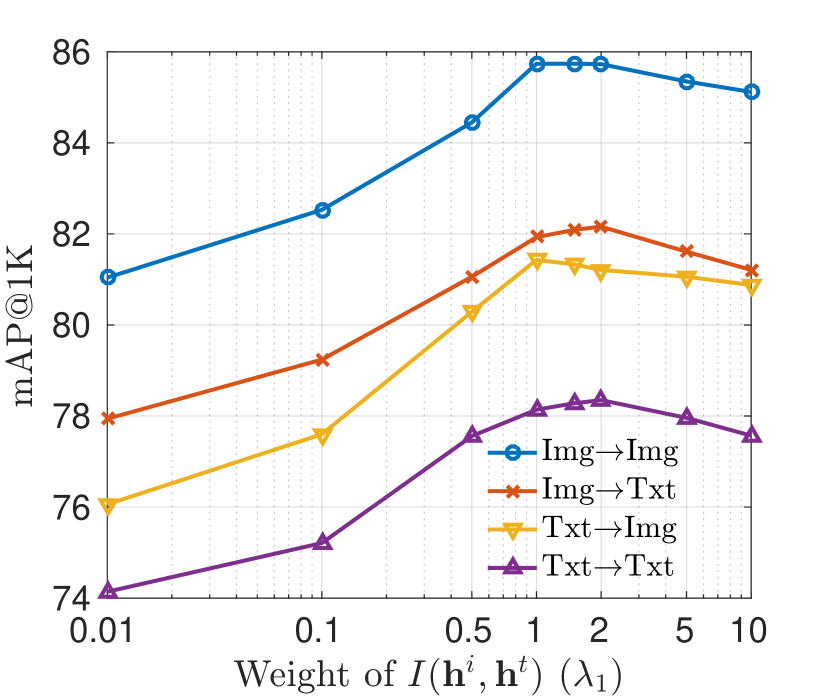
(a) MIR-Flickr25k

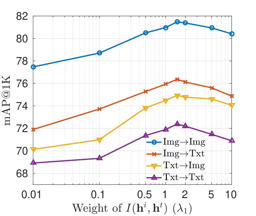
(b) NUS-WIDE

In this section, we conduct experiments on MIR-Flickr25k and NUS-WIDE datasets using 32-bit hash codes with various values of $I(\mathbf{h}^{i},\mathbf{h}^{t})$ weight (i.e., $\lambda_{1}$). The experimental results in term of mAP@1K are presented in Figure 1. As can be seen, when using a very small weight for $I(\mathbf{h}^{i},\mathbf{h}^{t})$ (i.e., $\lambda_{1}\leq 0.1$), the retrieval performance is significantly lower for all four retrieval tasks in compared with larger $I(\mathbf{h}^{i},\mathbf{h}^{t})$ weights (i.e., $\lambda_{1}\geq 1$). With a reasonable large weight for $I(\mathbf{h}^{i},\mathbf{h}^{t})$, the model is enforced to retain the information that is shared across modalities. The information that is shared among different modalities information is generally more useful for both the cross-modal and single-modal retrieval tasks; as, intuitively, this type of information is more likely to contain the ground-truth information. The experimental results confirm the importance and necessity of explicitly maximizing the mutual information between hash codes of different modalities. Besides, at a too large $I(\mathbf{h}^{{i}},\mathbf{h}^{{t}})$ weight (i.e., $\lambda_{1}\geq 5$), we also observe small decreases in retrieval performance. This fact is also understandable as the model pays less attention on maximizing $I(\mathbf{x}^{i},\mathbf{h}^{{i}})$ and $I(\mathbf{x}^{t},\mathbf{h}^{{t}})$, which results in less informative hash codes.

Figure 2: Histogram of $\boldsymbol{\mu}^{i}$ when using $T(\boldsymbol{\mu}^{i},\boldsymbol{\mu}^{t})$ and $T(\boldsymbol{h}^{{i}},\boldsymbol{h}^{{t}})$ (single pair of binary samples) for the MI lower bound estimator. The experiment is conducted on MIR-Flicrk25k with 32-bit hash codes. We observe similar histograms for $\boldsymbol{\mu}^{t}$.

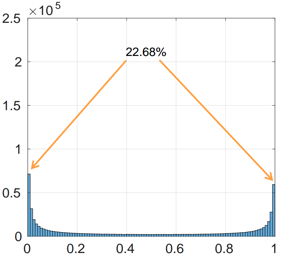
(a) $T(\boldsymbol{\mu}^{i},\boldsymbol{\mu}^{t})$

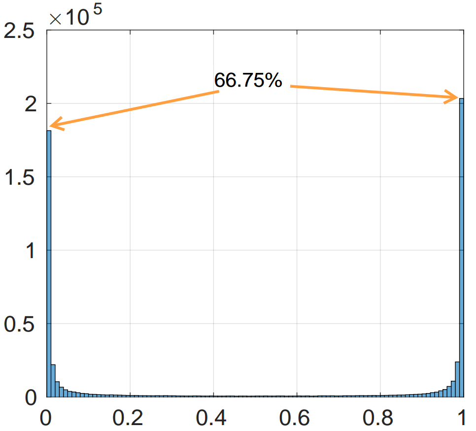
(b) $T(\boldsymbol{h}^{{i}},\boldsymbol{h}^{{t}})$

   

TABLE I: Cross-modal retrieval performance (mAP@1K (%)) with different input settings for function $T(\cdot)$ in estimating $I(\mathbf{h}^{{i}},\mathbf{h}^{{t}})$ lower bound. The experiment is conducted on MIR-Flicrk25k with 32 bit hash codes.

Task	$T(\boldsymbol{\mu}^{i},\boldsymbol{\mu}^{t})$	# of pairs of bin. samples for $T(\boldsymbol{h}^{{i}},\boldsymbol{h}^{{t}})$
		1	5	10	20
Img$\to$Txt	81.93	80.24	81.27	81.75	81.74
Txt$\to$Img	81.43	79.41	80.86	81.22	81.29

IV-B2 The benefit of using Bernoulli variables as the input of function $T$ in estimating $I(\mathbf{h}^{{i}},\mathbf{h}^{{t}})$ lower bound

In this section, we conduct experiments on MIR-Flickr25 dataset with $L=32$ bits to validate the benefit of using Bernoulli variables as the input of function $T$ in estimating $I(\mathbf{h}^{{i}},\mathbf{h}^{{t}})$ lower bound in comparison with using multiple pairs of binary samples as the input. The retrieval performance is presented in Table I. We also present the histograms of $\boldsymbol{\mu}^{i}$ when using $T(\boldsymbol{\mu}^{i},\boldsymbol{\mu}^{t})$ and $T(\boldsymbol{h}^{{i}},\boldsymbol{h}^{{t}})$ (with single sample) for the MI lower bound estimator in Figure 2. When using single pairs of binary samples as the input for the function $T(\boldsymbol{h}^{{i}},\boldsymbol{h}^{{t}})$, we can observe that the majority values of $\boldsymbol{\mu}^{i}$ become very small or very large. Approximate $67\%$ of $\boldsymbol{\mu}^{i}$ are in $[0,0.01]$ or $[0.99,1]$ (i.e., to be $0$ or $1$ respectively with $99\%$ confident), in comparison with about $22\%$ when using $T(\boldsymbol{\mu}^{i},\boldsymbol{\mu}^{t})$. This effect significantly affects the retrieval performance. When using multiple binary samples, the performance improves. However, the best performance is achieved when using Bernoulli variables. As this not only helps to eliminate input noise; but it also helps the gradients to not propagate through the biased gradient estimator STE, which introduces noise in gradients. Furthermore, we note that using $n$ binary samples would require approximately $n$-times computational cost.

IV-B3 Effect the symmetrized KL divergence

Figure 3: The mAP@1K (%) curves as the weight of $D_{\text{SKL}}$ varies on MIR-Flickr25k and NUS-WIDE using 32-bit hash codes.

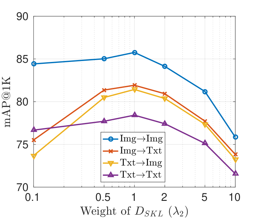
(a) MIR-Flickr25k

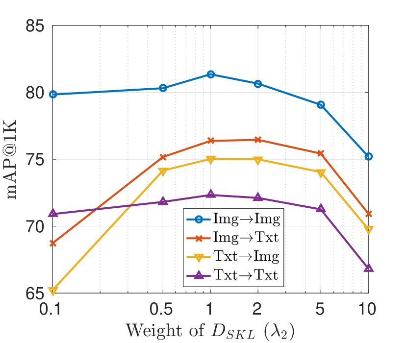
(b) NUS-WIDE

TABLE II: The TC, Corr MSE, and cross-modal retrieval performance (mAP@1K (%)) for MIR-Flickr25k dataset at different code lengths. ✓and ✗ indicate the hash codes are learned with and without $\mathcal{L}_{\text{ind}}$, respectively.

		16		32		48
		✓	✗	✓	✗	✓	✗
TC	Img	2.327	4.491	6.142	6.418	6.514	6.718
	Txt	2.174	4.288	6.015	6.424	6.425	6.645
Corr MSE	Img	0.037	0.068	0.040	0.092	0.051	0.078
	Txt	0.045	0.079	0.047	0.110	0.064	0.095
mAP@1K	Img$\to$Txt	80.68	80.39	81.93	81.38	82.92	82.16
	Txt$\to$Img	79.77	79.76	81.43	81.14	82.18	81.28

TABLE III: Comparison with state-of-the-art methods using mAP@1k (%) on three benchmark datasets.

Task	Method	MIR-Flickr25k			NUS-WIDE			MS-COCO
		16	32	48	16	32	48	16	32	48
Img$\to$Txt	CVH [23]	68.18	66.95	66.32	56.43	57.16	57.47	61.49	62.15	60.06
	PDH [24]	78.16	79.62	81.10	70.98	74.21	75.13	61.66	65.60	67.27
	CMFH [26]	77.97	78.69	78.50	69.13	70.96	71.18	59.21	64.62	66.55
	ACQ [28]	76.16	76.50	76.93	67.35	70.05	70.88	60.66	63.24	65.66
	FSH [29]	77.55	79.36	80.52	69.45	70.48	72.72	62.75	66.24	69.04
	DJSRH [38]	79.05	79.53	81.66	71.23	74.86	76.52	59.39	67.32	68.50
	CMIMH	80.68	81.93	82.92	73.92	76.37	77.21	65.32	69.21	70.20
Txt$\to$Img	CVH	68.08	66.89	66.40	57.40	58.30	58.51	62.45	63.46	61.22
	PDH	76.79	78.64	79.22	69.61	72.24	73.88	63.24	67.69	69.66
	CMFH	76.81	76.83	77.36	66.98	69.14	70.32	60.20	66.06	68.39
	ACQ	74.46	75.22	75.39	65.53	68.22	69.54	61.83	64.44	66.96
	FSH	75.10	77.10	78.47	67.59	69.03	70.25	65.05	69.07	71.48
	DJSRH	77.44	78.65	80.10	68.18	73.29	74.72	56.19	67.95	71.11
	CMIMH	79.77	81.43	82.18	72.75	75.02	75.68	66.08	70.35	72.21
Img$\to$Img	CVH	69.49	68.36	67.76	59.64	60.41	61.25	60.66	61.97	60.94
	PDH	79.65	81.46	82.86	74.23	77.06	78.08	61.10	65.28	67.06
	CMFH	81.45	82.54	83.13	75.33	77.72	78.35	60.31	65.53	67.78
	ACQ	78.91	78.94	79.58	71.13	76.63	74.88	60.07	62.46	64.76
	FSH	80.22	82.39	83.68	73.28	75.57	76.59	61.70	65.64	68.47
	DJSRH	82.39	83.17	84.07	77.29	79.29	80.27	59.87	66.77	68.29
	CMIMH	83.79	85.74	86.76	78.74	81.35	81.95	65.38	69.24	70.16
Txt$\to$Txt	CVH	67.47	66.79	66.72	57.45	60.13	61.50	64.17	66.84	64.96
	PDH	75.72	76.66	78.04	67.61	71.02	71.63	64.27	70.16	72.36
	CMFH	74.48	74.92	75.38	65.92	68.00	69.64	62.16	69.09	71.17
	ACQ	72.77	73.91	74.18	63.68	67.13	68.72	63.28	66.38	69.45
	FSH	73.35	75.03	76.28	65.89	67.55	69.10	67.05	72.78	75.67
	DJSRH	75.34	76.48	77.51	67.22	71.01	72.27	64.55	72.44	74.94
	CMIMH	77.36	78.42	79.01	70.18	72.33	72.72	68.15	73.28	74.89

In Figure 3, we present the mAP@1K curves as the weight of $D_{\text{SKL}}$ varies on the MIR-Flickr25k and NUS-WIDE datasets. Firstly, we can observe that too large weights for $D_{\text{SKL}}$ (i.e., $\lambda_{2}\geq 5$) have significant impacts on the retrieval performance for all four retrieval tasks. This observation is consistent with our discussion in Section III-C that too large $D_{\text{SKL}}$ weights will force the model to discard a large amount of modality-private information in the representations. As a result, the binary representations do not well-represent for the input data. For too small $D_{\text{SKL}}$ weights (i.e., $\lambda_{2}<0.5$), the retrieval performance on Img $\to$ Txt and Txt $\to$ Img retrieval tasks is unsurprisingly low as the binary representations of image and text modalities are poorly aligned with each other and not suitable for the cross-modal retrieval tasks. However, different from the case of too large $D_{\text{SKL}}$ weights, too small $D_{\text{SKL}}$ weights only result in minor performance drops for the Img $\to$ Img and Txt $\to$ Txt retrieval tasks, which means that the learned binary representations still well capture information of the input data. The small performance drops for the Img $\to$ Img and Txt $\to$ Txt retrieval tasks potentially indicate that the binary representations also capture information from the input data that does not share with the ground truth (e.g., noise).

IV-B4 The effectiveness of using Total Correlation (TC) as a regularizer to enhance hash bit independence

We conduct experiments on the MIR-Flickr25k dataset with and without the independence regularizer $\mathcal{L}_{\text{ind}}$. In Table II, we show the Mean Square Error (MSE) between the correlation matrix of the binary code of the database and the identity matrix (i.e., $\text{Corr~{}MSE}=\left\|\frac{1}{N}\hat{\mathbf{H}}^{\top}\hat{\mathbf{H}}-\mathbf{I}_{L}\right\|_{F}^{2}$, where $\hat{\mathbf{H}}=\{\hat{\mathbf{h}}_{j}\}_{j=1}^{N}\in\{-1,1\}^{N\times L}$ is the set of $L$-bit hash codes of a dataset and $\hat{\mathbf{h}}_{j}=2{\mathbf{h}}_{j}-1$) together with the retrieval performance at different code lengths. As can be seen, $\mathcal{L}_{\text{ind}}$ consistently helps to reduce the Corr MSEs for both image and text modalities at various code lengths. A smaller Corr MSE indicates that the hash bits are more independence and consequently leads to higher performance. Interestingly, we also notice that, at high code lengths, even though the classifiers can easily predict if a sample is from $q(z)$ with very high confident (i.e., high TC), $\mathcal{L}_{\text{ind}}$ is still helpful in reducing correlation between hash bits and improving performance.

TABLE IV: The cross-modal retrieval performance (mAP@1K (%)) for MIR-Flickr25k dataset to evaluate the effectiveness of each component in CMIMH. ✓and ✗ indicate the hash codes are learned with and without the according component, respectively. I$\to$T and T$\to$I mean Img$\to$Txt and Txt$\to$Img respectively.

Configuration				32 bits		48 bits
$I(\mathbf{h}^{{i}};\mathbf{h}^{{t}})$	$D_{\text{SKL}}$	$\mathcal{L}_{\text{ind}}$	$\mathcal{L}_{\text{bal}}$	I$\to$T	T$\to$I	I$\to$T	T$\to$I
✓	✗	✗	✗	75.13	73.14	77.57	75.49
✗	✓	✗	✗	77.61	75.53	78.89	78.39
✓	✗	✓	✓	75.52	73.69	77.84	75.83
✗	✓	✓	✓	77.87	75.95	79.34	78.69
✓	✓	✗	✗	81.28	80.73	82.07	81.51
✓	✓	✓	✗	81.35	80.93	82.11	81.82
✓	✓	✗	✓	81.43	81.14	82.16	81.78
✓	✓	✓	✓	81.93	81.43	82.92	82.18

IV-B5 A summary of effectiveness of different components

We additionally present in Table IV the cross-modal retrieval performance (mAP@1K (%)) for MIR-Flickr25k dataset with 32 and 48 bit hash codes with different combinations of components in the loss function. We can observe that the two terms $I(\mathbf{h}^{{i}};\mathbf{h}^{{t}})$ and $D_{\text{SKL}}(\mathbf{h}^{{i}};\mathbf{h}^{{t}})$ play very important roles in our proposed cross-modal hashing method. Without either $I(\mathbf{h}^{{i}};\mathbf{h}^{{t}})$ or $D_{\text{SKL}}(\mathbf{h}^{{i}};\mathbf{h}^{{t}})$ the cross-modal retrieval performance is significantly degraded. The ablation study also shows that the independence and balance terms are beneficial for hashing methods. However, even without these two terms, our proposed method CMIMH still achieves very good performance.

Figure 4: The Pre@K (%) curves on different datasets of 32-bit hash codes.

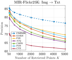
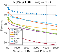
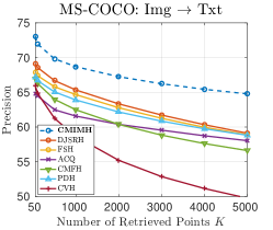
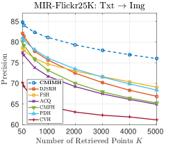
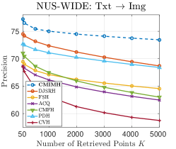
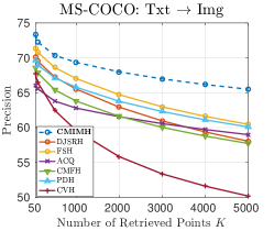
Figure 5: The Precision-Recall (PR) (%) curves on different datasets of 32-bit hash codes.

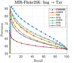
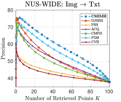
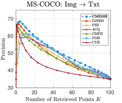
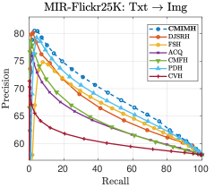
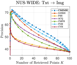
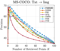
IV-C Comparison with the states of the art

In this section, we compare our proposed method against recent state-of-the-art cross-modal hashing methods, i.e., Cross-View Hashing (CVH) [23], Predictable Dualview Hashing (PDH) [24], Collective Matrix Factorization Hashing (CMFH) [26], Alternating Co-Quantization (ACQ) [28], Fusion Similarity Hashing (FSH) [29], and Deep Joint Semantics Reconstructing Hashing (DJSRH) [38]. From the experimental results in term of mAP@1k shown in Table III, we can observe that our proposed method outperforms the state-of-the-art unsupervised cross-modal hashing methods including the deep-based method (i.e., DJSRH) at majority of encoding lengths, datasets, and retrieval tasks. For the MS-COCO dataset with at $L=48$, CMIMH achieves lower performance than FSH and DJSRH on the Txt$\to$Txt retrieval tasks, while still outperforms DJSRH by clear margins in other settings.

Additionally, Figure 4 and Figure 5, respectively, show the Pre@K curves and Precision-Recall (PR) curves for Img$\to$Txt and Txt$\to$Img tasks with 32-bit hash codes. Compared with other methods, ours still significantly outperforms the state-of-the-art baselines over the three benchmark datasets for both metrics (i.e., Pre@K curves and PR curve). These results confirm the advantages of our proposed method in unsupervised cross-modal retrieval.

Comparison with Unsupervised Deep Cross Modal Hashing (UDCMH) [39] Following UDCMH, we report the mAP of top-50 retrieved results (mAP@50). The experiment results are shown in Table V. We observe that our proposed method can outperform UDCMH by large margins for both MIR-Flickr25k and NUS-WIDE datasets.

TABLE V: Comparison with UDCMH [39] using mAP@50 on MIR-FLickr25k and NUS-WIDE datasets. The results of UDCMH are cited from [39].

Task	Method	MIR-Flickr25k			NUS-WIDE
		16	32	64	16	32	64
Img$\to$	UDCMH	68.9	69.8	71.4	51.1	51.9	52.4
Txt	CMIMH	83.2	86.5	88.2	74.52	78.23	79.75
Txt$\to$	UDCMH	69.2	70.4	71.8	63.7	65.3	69.5
Img	CMIMH	82.4	83.8	86.2	73.89	76.08	79.14

TABLE VI: Comparison with MGAH [66] and UKD [87] using mAP (%) on MIR-Flickr25k and NUS-WIDE datasets. The results of MGAH and UKD are cited from original papers [66, 87].

Task	Method	MIR-Flickr25k			NUS-WIDE
		16	32	64	16	32	64
Img$\to$	MGAH	68.5	69.3	70.4	61.3	62.3	62.8
Txt	UKD-SS	71.4	71.8	72.5	61.4	63.7	63.8
	CMIMH	74.15	74.65	75.98	62.72	63.83	64.75
Txt$\to$	MGAH	67.3	67.6	68.6	60.3	61.4	64.0
Img	UKD-SS	71.5	71.6	72.1	63.0	65.6	65.7
	CMIMH	73.87	74.24	75.41	62.41	63.70	64.23

Comparison with Multi-pathway Generative Adversarial Hashing (MGAH) [66] and Unsupervised Knowledge Distillation for Cross-Modal Hashing (UKD) [87]: We conduct additional experiments on MIR-FLickr25k and NUS-WIDE datasets. For a fair comparison, we follow the experiment settings from [66] and [87]. Specifically, the FC7 features of the pretrained 19-layer VGGNet are used for images. 1,000-dimension BOW features are used for texts in both datasets. 1% samples of the NUS-WIDE dataset and 5% samples of the MIR-FLickr25k dataset are used as the query sets, and the rest as training set and also the retrieval database. We present the retrieval performance in term of mAP (of all retrieved samples) are shown in Table VI. We can observe that our proposed CMIMH consistently outperforms MGAH for both MIR-Flickr25k and NUS-WIDE datasets, especially for MIR-Flickr25k where the improvement gaps are greater than $5\%$. In comparison with UKD [87], our proposed method achieves lower performance on NUS-WIDE dataset - Txt$\to$Img task, while still outperform UKD on NUS-WIDE dataset - Img$\to$Txt task and MIR-Flickr25k for both tasks. These results show that our proposed method is still more favorable than UKD.

Comparison with Learning Disentangled Representation for Cross-Modal Retrieval with Deep Mutual Information Estimation (LDR) [70]: To have a fair comparison, we follow the experiment setting of [70]. Specifically, we extract VGG19 FC7 feature for images. We randomly select 1000 images as query, 1000 images as validation and the remaining images as database as well as training set. We report in Table VII the retrieval performance in term of RecallOne@K, the percent of queries for which the ground-truth is one of the first $K$ retrieved. In [70], the authors reported the RecallOne@K for 1024-dimension real-value features (32,768 bits), we find out that even with 128 bit hash codes, our proposed method can outperform LDR by large margins for both RecallOne@1 and RecallOne@10.

TABLE VII: Comparison with LDR [70] using RecallOne@K (%) on MS-COCO. The results of LDR are cited from [70].

Method	Img$\to$Txt		Img$\to$Txt
	$K=1$	$K=10$	$K=1$	$K=10$
LDR (1024-D)	53.4	91.3	40.5	88.7
CMIMH (128 bits)	65.53	94.35	69.82	93.32

Comparison with state of the art using hand-crafted image feature

Following the experiment setting of CRE [30] and FSH [29], we conduct experiments with hand-crafted features on NUS-WIDE datasets. For NUS-WIDE dataset, each image is represented by 500-dimensional BoW SIFT features and each text is represented by a 1,000-dimension preprocessed BOW feature. We randomly select 2,000 pairs as the query set; the remaining are used as the database. We also sample 20,000 pairs from the database as the training set. We present the experiment results in terms of mAP (of all returned samples) and Pre@100 (as used in [29, 30]) in Table VIII. We can observe that our proposed method can also work well with hand-crafted features and outperforms all compared methods.

TABLE VIII: Comparison using mAP (%) (of all returned samples) and Pre@100 on NUS-WIDE using hand-crafted features for images. The results of CRE method are cited from [30] and the results of other methods are cited from [29].

Task	Method	NUS-WIDE
		mAP			Pre@100
		16	32	64	32	64
Img$\to$Txt	CVH	38.11	36.85	35.74	47.49	43.87
	PDH	46.58	47.47	47.80	49.89	51.25
	CMFH	37.23	37.81	37.99	50.64	53.09
	ACQ	42.47	44.35	43.28	44.42	43.09
	FSH [29]	50.59	50.63	51.71	52.97	56.16
	CRE [30]	51.31	52.99	53.32	-	-
	CMIMH	53.66	53.95	55.34	63.98	65.68
Txt$\to$Img	CVH	37.68	36.52	35.55	46.90	43.21
	PDH	44.58	45.19	45.52	51.33	52.84
	CMFH	39.57	40.36	41.05	45.17	45.95
	ACQ	41.34	42.73	42.00	45.73	48.87
	FSH	47.90	48.10	49.65	53.88	56.85
	CRE	49.27	50.86	51.49	-	-
	CMIMH	53.01	53.44	55.19	60.77	61.37

Effect of training size

Different from most of the state-of-the-art methods [23, 24, 26, 28, 29, 39], our proposed method can be fully-optimized using gradient descent in a mini-batch manner. Therefore, our proposed method can be easily trained with much larger training sets. We further analyze the effects on retrieval performance when varying the training size on NUS-WIDE dataset. We also compare our retrieval performance with the retrieval performance of DJSRH [38], which is one of our most competitive methods and also can be trained in a mini-batch manner. The retrieval performance in term of mAP@1k when using different training set sizes are shown in Table IX. We can observe that our proposed method can achieve higher mAP@1k when utilizing more training data. Furthermore, our proposed method also consistently outperforms DJSRH [38] with different training sizes.

TABLE IX: The cross-modal retrieval performance in term of mAP@1k (%) on the NUS-WIDE dataset with different numbers of training samples.

L	Task	Method	Training size
			5k	10k	20k
16	Img$\to$Txt	DJSRH [38]	71.23	72.67	73.46
		CMIMH	73.59	75.14	77.25
	Txt$\to$Img	DJSRH	68.18	71.12	73.53
		CMIMH	73.39	75.45	76.54
32	Img$\to$Txt	DJSRH	74.86	76.93	77.58
		CMIMH	76.20	77.80	79.06
	Txt$\to$Img	DJSRH	73.29	74.97	77.31
		CMIMH	74.88	76.46	78.23
48	Img$\to$Txt	DJSRH	76.52	78.17	78.78
		CMIMH	76.71	78.62	79.66
	Txt$\to$Img	DJSRH	74.72	77.35	77.29
		CMIMH	75.98	78.12	78.81

V Conclusion

In this paper, inspired by recent advances in learning representation by maximizing mutual information, we proposed a novel framework, dubbed Cross-Modal Info-Max Hashing (CMIMH). By assuming the binary representations to be modeled by multivariate Bernoulli distributions, we can maximize the MI effectively using gradient descent optimization in a mini-batch manner via maximizing their estimated variational lower-bounds. We additionally find out that trying to minimize modality gap by learning similar binary representations for the same instance from different modalities could result in modality-private information loss. Properly balancing the modality gap and modality-private information loss is important to achieve better performance. Experiment results confirm the effectiveness of our proposed method for both cross-modal and single-modal retrieval tasks. Additionally, the ablation studies clearly justify the advantages of different components in our proposed method.

References

- [1] Y. Zhen and D.-Y. Yeung, “Co-regularized hashing for multimodal data,” in NIPS, 2012, pp. 1376–1384.
- [2] Y. Wei, Y. Song, Y. Zhen, B. Liu, and Q. Yang, “Heterogeneous translated hashing: A scalable solution towards multi-modal similarity search,” ACM Trans. Knowl. Discov. Data, vol. 10, no. 4, 2016.
- [3] D. Zhangy and W.-J. Li, “Large-scale supervised multimodal hashing with semantic correlation maximization,” in AAAI, 2014.
- [4] B. Wu, Q. Yang, W.-S. Zheng, Y. Wang, and J. Wang, “Quantized correlation hashing for fast cross-modal search,” in IJCAI, 2015.
- [5] Z. Lin, G. Ding, Mingqing Hu, and J. Wang, “Semantics-preserving hashing for cross-view retrieval,” in CVPR, 2015.
- [6] X. Xu, F. Shen, Y. Yang, H. T. Shen, and X. Li, “Learning discriminative binary codes for large-scale cross-modal retrieval,” IEEE TIP, vol. 26, no. 5, pp. 2494–2507, 2017.
- [7] Q. Jiang and W. Li, “Discrete latent factor model for cross-modal hashing,” IEEE TIP, vol. 28, no. 7, pp. 3490–3501, 2019.
- [8] J. Tang, K. Wang, and L. Shao, “Supervised matrix factorization hashing for cross-modal retrieval,” IEEE Transactions on Image Processing, vol. 25, no. 7, 2016.
- [9] D. Mandal, K. N. Chaudhury, and S. Biswas, “Generalized semantic preserving hashing for cross-modal retrieval,” IEEE TIP, vol. 28, no. 1, pp. 102–112, Jan 2019.
- [10] C. Deng, Z. Chen, X. Liu, X. Gao, and D. Tao, “Triplet-based deep hashing network for cross-modal retrieval,” IEEE TIP, vol. 27, no. 8, pp. 3893–3903, Aug 2018.
- [11] Z. Cao, M. Long, J. Wang, and Q. Yang, “Transitive hashing network for heterogeneous multimedia retrieval,” in AAAI, 2017.
- [12] Q. Jiang and W. Li, “Deep cross-modal hashing,” in CVPR, July 2017.
- [13] Z.-D. Chen, W.-J. Yu, C.-X. Li, L. Nie, and X.-S. Xu, “Dual deep neural networks cross-modal hashing,” in AAAI, 2018.
- [14] V. E. Liong, J. Lu, Y. Tan, and J. Zhou, “Cross-modal deep variational hashing,” in ICCV, 2017.
- [15] E. Yang, C. Deng, W. Liu, X. Liu, D. Tao, and X. Gao, “Pairwise relationship guided deep hashing for cross-modal retrieval,” in AAAI, 2017.
- [16] Y. Cao, M. Long, J. Wang, Q. Yang, and P. S. Yu, “Deep visual-semantic hashing for cross-modal retrieval,” in ACM SIGKDD International Conference on Knowledge Discovery and Data Mining, 2016.
- [17] C. Li, T. Yan, X. Luo, L. Nie, and X. Xu, “Supervised robust discrete multimodal hashing for cross-media retrieval,” IEEE TMM, vol. 21, no. 11, pp. 2863–2877, 2019.
- [18] G. Song, D. Wang, and X. Tan, “Deep Memory Network for Cross-Modal Retrieval,” IEEE TMM, vol. 21, no. 5, pp. 1261–1275, 2019.
- [19] D. Xie, C. Deng, C. Li, X. Liu, and D. Tao, “Multi-Task Consistency-Preserving Adversarial Hashing for Cross-Modal Retrieval,” IEEE TIP, vol. 29, pp. 3626–3637, 2020.
- [20] L. Jin, K. Li, Z. Li, F. Xiao, G.-J. Qi, and J. Tang, “Deep semantic-preserving ordinal hashing for cross-modal similarity search,” IEEE Transactions on Neural Networks and Learning Systems, vol. 30, no. 5, pp. 1429–1440, 2019.
- [21] B. Wang, Y. Yang, X. Xu, A. Hanjalic, and H. T. Shen, “Adversarial cross-modal retrieval,” in ACM Multimedia, 2017.
- [22] F. Wu, X.-Y. Jing, Z. Wu, Y. Ji, X. Dong, X. Luo, Q. Huang, and R. Wang, “Modality-specific and shared generative adversarial network for cross-modal retrieval,” Pattern Recognition, vol. 104, p. 107335, 2020.
- [23] S. Kumar and R. Udupa, “Learning hash functions for cross-view similarity search,” in IJCAI, 2011.
- [24] M. Rastegari, J. Choi, S. Fakhraei, D. Hal, and L. Davis, “Predictable dual-view hashing,” in ICML, 2013.
- [25] J. Song, Y. Yang, Y. Yang, Z. Huang, and H. T. Shen, “Inter-media hashing for large-scale retrieval from heterogeneous data sources,” in ACM SIGMOD, 2013.
- [26] G. Ding, Y. Guo, J. Zhou, and Y. Gao, “Large-scale cross-modality search via collective matrix factorization hashing,” IEEE TIP, vol. 25, 2016.
- [27] J. Zhou, G. Ding, and Y. Guo, “Latent semantic sparse hashing for cross-modal similarity search,” in ACM SIGIR, 2014.
- [28] G. Irie, H. Arai, and Y. Taniguchi, “Alternating co-quantization for cross-modal hashing,” in ICCV, 2015.
- [29] H. Liu, R. Ji, Y. Wu, F. Huang, and B. Zhang, “Cross-modality binary code learning via fusion similarity hashing,” in CVPR, 2017.
- [30] M. Hu, Y. Yang, F. Shen, N. Xie, R. Hong, and H. T. Shen, “Collective reconstructive embeddings for cross-modal hashing,” IEEE TIP, vol. 28, no. 6, pp. 2770–2784, June 2019.
- [31] D. Wang, P. Cui, M. Ou, and W. Zhu, “Learning compact hash codes for multimodal representations using orthogonal deep structure,” IEEE TMM, vol. 17, no. 9, 2015.
- [32] W. Wang, B. C. Ooi, X. Yang, D. Zhang, and Y. Zhuang, “Effective multi-modal retrieval based on stacked auto-encoders,” VLDB Endowment, vol. 7, no. 8, 2014.
- [33] F. Feng, X. Wang, and R. Li, “Cross-modal retrieval with correspondence autoencoder,” in ACM Multimedia, 2014.
- [34] J. G. Zhang, Y. Peng, and M. Yuan, “Unsupervised generative adversarial cross-modal hashing,” in AAAI, 2018.
- [35] J. Guo and W. Zhu, “Collective affinity learning for partial cross-modal hashing,” IEEE TIP, vol. 29, pp. 1344–1355, 2020.
- [36] L. Wang, W. Sun, Z. Zhao, and F. Su, “Modeling intra- and inter-pair correlation via heterogeneous high-order preserving for cross-modal retrieval,” Signal Processing, vol. 131, pp. 249–260, 2017.
- [37] T. Hoang, T.-T. Do, T. V. Nguyen, and N.-M. Cheung, “Unsupervised Deep Cross-modality Spectral Hashing,” IEEE TIP, vol. 29, pp. 8391–8406, 2020.
- [38] S. Su, Z. Zhong, and C. Zhang, “Deep joint-semantics reconstructing hashing for large-scale unsupervised cross-modal retrieval,” in ICCV, 2019.
- [39] G. Wu, Z. Lin, J. Han, L. Liu, G. Ding, B. Zhang, and J. Shen, “Unsupervised deep hashing via binary latent factor models for large-scale cross-modal retrieval,” in IJCAI, 2018.
- [40] X. Zhu, Z. Huang, H. T. Shen, and X. Zhao, “Linear cross-modal hashing for efficient multimedia search,” in ACM Multimedia, 2013, p. 143–152.
- [41] D. Wang, Q. Wang, and X. Gao, “Robust and flexible discrete hashing for cross-modal similarity search,” IEEE Transactions on Circuits and Systems for Video Technology, vol. 28, no. 10, pp. 2703–2715, Oct 2018.
- [42] C. Li, C. Deng, L. Wang, D. Xie, and X. Liu, “Coupled CycleGAN: Unsupervised Hashing Network for Cross-Modal Retrieval,” in AAAI, 2019.
- [43] R. D. Hjelm, A. Fedorov, S. Lavoie-Marchildon, K. Grewal, P. Bachman, A. Trischler, and Y. Bengio, “Learning deep representations by mutual information estimation and maximization,” in ICLR, 2019.
- [44] A. van den Oord, Y. Li, and O. Vinyals, “Representation learning with contrastive predictive coding,” 2018. [Online]. Available: http://arxiv.org/abs/1807.03748
- [45] P. Bachman, R. D. Hjelm, and W. Buchwalter, “Learning Representations by Maximizing Mutual Information Across Views,” in NeurIPS, 2019, pp. 15 535–15 545.
- [46] M. Federici, A. Dutta, P. Forré, N. Kushman, and Z. Akata, “Learning robust representations via multi-view information bottleneck,” in ICLR, 2020.
- [47] D. Barber and F. Agakov, “The im algorithm: A variational approach to information maximization.” in NIPS, 2003.
- [48] X. Chen, Y. Duan, R. Houthooft, J. Schulman, I. Sutskever, and P. Abbeel, “Infogan: Interpretable representation learning by information maximizing generative adversarial nets,” in NIPS, 2016.
- [49] S. Nowozin, B. Cseke, and R. Tomioka, “f-gan: Training generative neural samplers using variational divergence minimization,” in NIPS, 2016.
- [50] M. I. Belghazi, A. Baratin, S. Rajeshwar, S. Ozair, Y. Bengio, A. Courville, and D. Hjelm, “Mutual information neural estimation,” in ICML, 2018.
- [51] X. Nguyen, M. J. Wainwright, and M. I. Jordan, “Estimating divergence functionals and the likelihood ratio by convex risk minimization,” IEEE Transactions on Information Theory, vol. 56, no. 11, p. 5847–5861, 2010.
- [52] Y. Weiss, A. Torralba, and R. Fergus, “Spectral hashing,” in NIPS, 2008.
- [53] Y. Gong, S. Lazebnik, A. Gordo, and F. Perronnin, “Iterative quantization: A procrustean approach to learning binary codes for large-scale image retrieval,” IEEE TPAMI, vol. 35, no. 12, 2013.
- [54] J. Wang, S. Kumar, and S. Chang, “Semi-supervised hashing for scalable image retrieval,” in CVPR, 2010, pp. 3424–3431.
- [55] T.-T. Do, D. L. Tan, T. T. Pham, and N. Cheung, “Simultaneous feature aggregating and hashing for large-scale image search,” in CVPR, 2017.
- [56] T.-T. Do, T. Hoang, D.-K. Le Tan, A.-D. Doan, and N.-M. Cheung, “Compact Hash Code Learning With Binary Deep Neural Network,” IEEE TMM, vol. 22, no. 4, pp. 992–1004, 2020.
- [57] T. Hoang, T.-T. Do, H. Le, D.-K. Le-Tan, and N.-M. Cheung, “Simultaneous compression and quantization: A joint approach for efficient unsupervised hashing,” CVIU, vol. 191, 2020.
- [58] W. Satosi, “Information theoretical analysis of multivariate correlation,” IBM Journal of research and development, vol. 4, no. 1, pp. 66–82, 1960.
- [59] C. Li, C. Deng, N. Li, W. Liu, X. Gao, and D. Tao, “Self-supervised adversarial hashing networks for cross-modal retrieval,” in CVPR, 2018.
- [60] V. E. Liong, J. Lu, L. yu Duan, and Y. Tan, “Deep variational and structural hashing,” IEEE TPAMI, vol. 42, pp. 580–595, 2020.
- [61] Y. Cao, B. Liu, M. Long, and J. Wang, “Cross-Modal Hamming Hashing,” in ECCV, 2018, pp. 207–223.
- [62] Z. Ji, Y. Sun, Y. Yu, Y. Pang, and J. Han, “Attribute-guided network for cross-modal zero-shot hashing,” IEEE TNNLS, vol. 31, no. 1, pp. 321–330, 2020.
- [63] X. Bai, S. Bai, and X. Wang, “Beyond diffusion process: Neighbor set similarity for fast re-ranking,” Information Sciences, vol. 325, 2015.
- [64] K. Wang, Q. Yin, W. Wang, S. Wu, and L. Wang, “A comprehensive survey on cross-modal retrieval,” CoRR, vol. abs/1607.06215, 2016.
- [65] D. Hu, F. Nie, and X. Li, “Deep binary reconstruction for cross-modal hashing,” IEEE Transactions on Multimedia, 2018.
- [66] J. Zhang and Y. Peng, “Multi-Pathway Generative Adversarial Hashing for Unsupervised Cross-Modal Retrieval,” IEEE TMM, vol. 22, no. 1, pp. 174–187, 2020.
- [67] L. Wu, Y. Wang, and L. Shao, “Cycle-consistent deep generative hashing for cross-modal retrieval,” IEEE TIP, vol. 28, no. 4, pp. 1602–1612, 2019.
- [68] J.-Y. Zhu, T. Park, P. Isola, and A. A. Efros, “Unpaired image-to-image translation using cycle-consistent adversarial networks,” in ICCV, 2017.
- [69] F. Cakir, K. He, S. Adel Bargal, and S. Sclaroff, “Mihash: Online hashing with mutual information,” in ICCV, 2017.
- [70] W. Guo, H. Huang, X. Kong, and R. He, “Learning Disentangled Representation for Cross-Modal Retrieval with Deep Mutual Information Estimation,” in ACM Multimedia, 2019, pp. 1712–1720.
- [71] J. Hu, R. Ji, S. Zhang, X. Sun, Q. Ye, C.-W. Lin, and Q. Tian, “Information Competing Process for Learning Diversified Representations,” in Advances in Neural Information Processing Systems, 2019.
- [72] Y. Tian, D. Krishnan, and P. Isola, “Contrastive Representation Distillation,” in ICLR, 2020.
- [73] ——, “Contrastive multiview coding,” arXiv preprint arXiv:1906.05849, 2019.
- [74] A. A. Alemi, I. Fischer, J. V. Dillon, and K. Murphy, “Deep variational information bottleneck,” in ICLR, 2017.
- [75] N. Tishby, F. C. Pereira, and W. Bialek, “The information bottleneck method,” 2000.
- [76] C. J. Maddison, A. Mnih, and Y. W. Teh, “The concrete distribution: A continuous relaxation of discrete random variables,” in ICLR, 2017.
- [77] G. Tucker, A. Mnih, C. J. Maddison, J. Lawson, and J. Sohl-Dickstein, “Rebar: Low-variance, unbiased gradient estimates for discrete latent variable models,” in NIPS, 2017.
- [78] G. Hinton, “Neural networks for machine learning,” Coursera, video lectures, 2012.
- [79] B. Poole, S. Ozair, A. Van Den Oord, A. Alemi, and G. Tucker, “On variational bounds of mutual information,” in ICML, 2019, pp. 5171–5180.
- [80] M. D. Donsker and S. R. S. Varadhan, “Asymptotic evaluation of certain markov process expectations for large time, i,” Communications on Pure and Applied Mathematics, vol. 28, no. 1, pp. 1–47, 1975.
- [81] H. Kim and A. Mnih, “Disentangling by factorising,” in ICML, 2018.
- [82] M. J. Huiskes and M. S. Lew, “The MIR Flickr retrieval evaluation,” in ACM International Conference on Multimedia Information Retrieval, 2008.
- [83] T. seng Chua, J. Tang, R. Hong, H. Li, Z. Luo, and Y. Zheng, “NUS-WIDE: A real-world web image database from National University of Singapore,” in CIVR, 2009.
- [84] T. Lin, M. Maire, S. J. Belongie, L. D. Bourdev, R. B. Girshick, J. Hays, P. Perona, D. Ramanan, P. Dollár, and C. L. Zitnick, “Microsoft COCO: common objects in context,” in ECCV, 2014.
- [85] J. Devlin, M. Chang, K. Lee, and K. Toutanova, “BERT: pre-training of deep bidirectional transformers for language understanding,” arXiv, vol. abs/1810.04805, 2018.
- [86] A. Krizhevsky, I. Sutskever, and G. E. Hinton, “Imagenet classification with deep convolutional neural networks,” in NeurIPS, 2012.
- [87] H. Hu, L. Xie, R. Hong, and Q. Tian, “Creating Something From Nothing: Unsupervised Knowledge Distillation for Cross-Modal Hashing,” in CVPR, 2020, pp. 3120–3129.