A further analysis for galactic dark matter halos with pressure

Abstract

Spherically symmetric and static dark matter halos in hydrostatic equilibrium demand that dark matter should have an effective pressure that compensates the gravitational force of the mass of the halo. An effective equation of state can be obtained for each rotational velocity profile of the stars in galaxies. In this work, we study one of this dark matter equation of state obtained for the Universal Velocity Profile and analyze the properties of the self-gravitating structures that emerges from this equation of state. The resulting configurations explaining the observed rotational speeds are found to be unstable. We conclude that either the halo is not in hydrostatic equilibrium, or it is non spherically symmetric, or it is not static if the Universal Velocity profile should be valid to fit the rotational velocity curve of the galaxies.

1 Introduction

Current astrophysical observations at cosmological and galactic scales suggest a concordance standard model coined Lambda Cold Dark Matter ($\Lambda$-CDM) [Aghanim, 2018]. It contains three major components: a cosmological constant $\Lambda$, a cold dark matter component (CDM), and ordinary matter. We don’t know much about this invisible component named CDM that acts gravitationally on baryonic matter, being the observed rotational curves of spiral galaxies one of the most direct evidence of its existence [Sofue, 2000]. It is not known what it is made of but there is the belief that it is a pressureless medium which dominates in the outer regions of spiral galaxies. While luminous matter dominates in the innermost regions of galaxies, it appears that the effects of dark matter can also be found in regions where ordinary matter is present [Persic, 1996]. The pressureless condition of CDM leads to a background cosmological evolution of its density that varies as $a^{-3}$, being $a$ the scale factor of the universe. Latest satellite missions WMAP and Planck have promoted cosmology to a new precision era where the hypothesis of pressureless dark matter can be tested [Muller, 2004, Serra, 2011, Calabrese, 2009, Xu, 2013, Yang, 2015, Kopp, 2018]. In particular, it has been found that a barotropic equation of state for the dark matter, $p_{DM}=\omega_{DM}~{}\rho$, with $\omega_{DM}=0.000707^{+0.000747}_{-0.000746}$ is compatible with the evolution of the Universe [Xu, 2013, Yang, 2015, Kopp, 2018], hence compatible with the pressureless CDM hypothesis.

Nevertheless, at galactic scales it is known that $\Lambda$-CDM is unable to provide a complete description of the dark matter halos [Weinberg, 2015, Perivolaropoulos, 2021]. The core-cusp problem [Flores, 1994, Karukes, 2015], the too big to fail problem [Boylan-Kolchin, 2011] and the missing satellite problem [Klypin, 1999, Moore, 1999], among others, force us to carefully reconsider the pressureless dark matter hypothesis. It is known that self-interacting dark matter could solve some small scale problems of $\Lambda$-CDM [Spergel, 1999]. The strength of self-interaction between dark matter particles leads to some effective pressure. Moreover, dark matter must have pressure in order to avoid that intermediate-mass black holes increase their mass far beyond observations due to dark mater accretion [Pepe, 2011, Lora-Clavijo, 2014]. This junction, between the actual observational capability for testing the pressureless hypothesis of dark matter and the current problems of $\Lambda$-CDM to explain some issues at galactic scales, is a strong motivation to study the possibility that dark matter has some pressure.

Considering the rotational curves of galaxies in Barranco [2013], it was shown that given a velocity profile $v_{t}$ for test particles in a spherically symmetric and static dark matter halo in hydrostatic equilibrium, the gravitational potential $\Phi$ is fixed by $v_{t}$. If the dark matter in the halo is modeled as a perfect fluid, once the gravitational potential is fixed, then the hydrostatic equilibrium equations automatically determine an effective equation of state, $p(\rho)\neq 0$, for dark matter. In this way, several equations of state (EoS) were obtained in Barranco [2013]. Each EoS corresponds to a different velocity profile. The present work explores in more detail one of those EoS by analyzing the structure of the resulting dark matter halos obtained as self-gravitating structures of a perfect fluid that models dark matter with such EoS. In particular, the EoS we are going to explore is the one that is obtained using the universal rotational velocity profile studied by Persic and Salucci in Persic [1996]. In this case, the EoS is given by Barranco [2013]

$$\rho(p)=\frac{\rho_{\bullet}}{6}\left(1+8\frac{p}{p_{\bullet}}-\sqrt{1+8\frac{p}{p_{\bullet}}}\right),$$ (1)

where $\rho_{\bullet}$ and $p_{\bullet}$ are free parameters. For a given set of values for this two parameters, the resulting dark matter halos show several deficiencies in order to be astrophysical reasonable dark matter halos, namely:

• The radial density decays as $\rho(r)\sim 1/r^{2}$ and extends to infinity.

• The total mass of the resulting dark matter halo grows linearly in $r$.

• The resulting self-gravitating configurations that produce rotational curves that fit the observational data are in the branch of unstable configurations.

The first two shortcomings can be resolved by defining the dark matter halo radius where the halo density equals the average density of the universe. The problem of the instability of the halo implies that at least one of our assumptions is incorrect: either the halo is not in hydrostatic equilibrium, or it is not spherically symmetric, or it is not static, or dark matter is not a perfect fluid.

In order to show how these conclusions are attained, the article is organized as follows: Section 2 reviews the TOV equations and explains the EoS (equation 1) analyzed in this work. Section 3 details the numerical methods here employed and shows the resulting self-gravitating structures obtained, as well as, their main properties. Section 4 is devoted to some discussions and then Section 5 is for the conclusions regarding the obtained results.

2 Self-gravitating perfect fluid as a dark matter halo

Dark matter will be treated as a perfect fluid defined by stresses $T^{r}_{r}=T^{\theta}_{\theta}=T^{\phi}_{\phi}=p$, $T^{t}_{t}=-\rho$, being $p$, $\rho$ the pressure and the density of the fluid, respectively. The rest of the stresses are zero. Galaxies are composed of luminous matter encapsulated by a dark matter halo. Observation of carbon giant stars in the Galactic halo implies that the dark matter halo of our galaxy is spherically symmetric [Ibata, 2000]. Since our galaxy is not special, it seems reasonable to assume that most dark matter halos are spherically symmetric and thus we will assume such symmetry. Since the amount of luminous matter compared with the amount of dark matter in Low Surface Brightness (LSB) galaxies is small, thus baryonic matter does not contribute significantly to the total mass for such galaxies. Therefore, the halo for LSB galaxies can be modeled by a self-gravitating sphere of perfect dark matter fluid in hydrostatic equilibrium. In this section, we present the equations that will describe such self-gravitating structure: the Tolman-Oppenheimer-Volkov equations and the dark matter EoS.

2.1 Tolman-Oppenheimer-Volkov equations

First, we recall the well known general relativistic Tolman-Oppenheimer-Volkov (TOV) equations [Tolman, 1939, Oppenheimer, 1939] (see also Silbar [2004]), which are the main theoretical tool used in the present work. We consider a static and spherically symmetric spacetime, whose line element in Schwarzschild coordinates is

$$ds^{2}=-e^{2\Phi}c^{2}dt^{2}+\frac{dr^{2}}{(1-\frac{2Gm}{c^{2}r})}+r^{2}(d\theta^{2}+\sin^{2}\theta\,d\phi^{2}),$$ (2)

being $m$ and $\Phi$ functions of only the radial coordinate $r$. We think of $m$ as the gravitational mass inside the sphere of radius $r$ and $\Phi$ can be interpreted as the Newtonian gravitational potential. If the matter content of the spacetime is a perfect fluid, then the Einstein field equations imply the TOV system of equations:

$$\frac{dm}{dr}=4\pi r^{2}\rho,$$ (3)

$$\frac{dp}{dr}=-\frac{Gm\rho}{r^{2}}\frac{\left(1+\frac{p}{c^{2}\rho}\right)\left(1+\frac{4\pi r^{3}p}{mc^{2}}\right)}{1-\frac{2Gm}{c^{2}r}}.$$ (4)

These equations express the equilibrium at each $r$, between the internal pressure that the material supports against the attraction of the gravitational mass within $r$. These are the hydrostatic equilibrium equations in General Relativity, where the factor $\frac{2Gm}{c^{2}r}$, that appears in the equation (4), determines whether the effects of General Relativity should be taken into account or not. When $\frac{2Gm}{c^{2}r}\ll 1$ we can neglect this term in the TOV system and we arrive at the corresponding well-known Newtonian limit:

$$\frac{dm}{dr}=4\pi r^{2}\rho,\quad\frac{dp}{dr}=-\frac{Gm\rho}{r^{2}}.$$ (5)

It is convenient for the discussion and numerical integration to use dimensionless quantities,

$$\bar{m}=\frac{m}{M_{\star}},\quad\bar{r}=\frac{r}{R_{\star}},\quad\bar{\rho}=\frac{\rho}{\rho_{\star}},\quad\bar{p}=\frac{p}{p_{\star}},$$ (6)

where $M_{\star}$ and $R_{\star}$ are the characteristic scales for mass and distance of the system under study. In Barranco [2013], they are taken to be

$$M_{\star}=10^{10}M_{\odot},\qquad R_{\star}=1\,kpc.$$ (7)

Also, the characteristic density and pressure are

$$\rho_{\star}=\frac{M_{\star}}{\frac{4}{3}\pi R_{\star}^{3}},\qquad p_{\star}=c^{2}\rho_{\star},$$ (8)

which give the values

$$\rho_{\star}=1.66\times 10^{-22}\frac{g}{cm^{3}},\qquad p_{\star}=1.49\times 10^{-1}\frac{g}{cm\,s^{2}}.$$ (9)

In terms of these quantities equations 3-4 take the form

$$\frac{d\bar{m}}{d\bar{r}}=3\bar{r}^{2}\bar{\rho},$$ (10)

$$\frac{d\bar{p}}{d\bar{r}}=-G_{\star}\frac{\bar{m}\bar{\rho}}{\bar{r}^{2}}\left(1+\frac{\bar{p}}{\bar{\rho}}\right)\left(1+\frac{3\bar{r}^{3}\bar{p}}{\bar{m}}\right)\left(1-2G_{\star}\frac{\bar{m}}{\bar{r}}\right)^{-1},$$ (11)

with

$$G_{\star}=\frac{GM_{\star}}{c^{2}R_{\star}}=4.785\times 10^{-7}.$$ (12)

The system of equations 10-11 is formally singular at $\bar{r}=0$, being $\bar{p}(\bar{r}=0)=\bar{p}_{0}$ the only free parameter. To perform the numerical integration of these equations, we make use of the Taylor expansions for $\bar{m}$ and $\bar{p}$:

$$\bar{m}(\bar{r})=\bar{\rho}(\bar{p}_{0})\bar{r}^{3}+O(\bar{r}^{5}),$$ (13)

$$\bar{p}(\bar{r})=\bar{p}_{0}+\frac{\bar{p}_{2}}{2}\bar{r}^{2}+O(\bar{r}^{3}),$$ (14)

with

$$\bar{p}_{2}=-G_{\star}\left[\bar{\rho}(\bar{p}_{0})+3\bar{p}_{0}\right]\left[\bar{\rho}(\bar{p}_{0})+\bar{p}_{0}\right].$$ (15)

Then, given an EoS of the form $\bar{\rho}=\bar{\rho}(\bar{p})$, the family of solutions is parametrized by the central pressure $\bar{p}_{0}$, which is equivalent to get it parametrized by the central density $\bar{\rho}(\bar{r}=0)=\bar{\rho}_{0}$. In order to close the TOV system an EoS is needed, to describe the matter content of the spherical halo.

2.2 Velocity profile and phenomenological EoS for dark matter

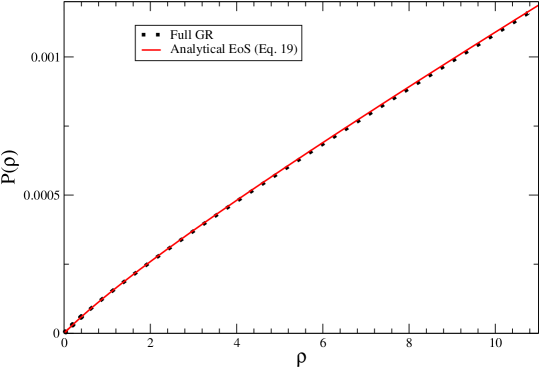
Figure 1: Comparison of the EoS obtained using the full general relativistic approach (dotted line) against the approximate solution obtained in the Newtonian approximation given by equation 21.

The quest to determine the nature of dark matter is perhaps one of the most challenging problems in modern physics. The particle physics approach is the most dominant in the literature. It consists in proposing a dark matter candidate that heals some standard particle model problems as well as to provide a viable weakly interacting particle that plays the role of dark matter. Well motivated examples of such dark matter candidates are the neutralino (the lightest stable neutral supersymmetric particle) or the axion (a pseudoscalar boson that solves the Strong CP problem).

On the other hand, an approach where stellar dynamics and a collection of reduced hypothesis determine general properties of dark matter, is not the mainstream. Fluid dark matter models represent an example of such phenomenological approach. In particular, the rotational velocity profiles of galaxies can provide important insights about dark matter under this fluid approach. For instance, in Barranco [2013] several velocity rotational profiles of galaxies were considered to construct EoS for dark matter. Actually, what is shown in Barranco [2013] is that if dark matter behaves as a perfect fluid, imposing the spacetime to be spherically symmetric and static, and given a profile of rotational velocities $v_{t}(r)$ of stars in a galaxy, thus, dark matter halos in hydrostatic equilibrium demand an effective EoS. The argument is simple enough: for a spherically symmetric and static spacetime, for test particles in circular motion, there is a relationship between tangential velocity and the gravitational potential $\Phi$, given by $\Phi^{\prime}(r)=v_{t}^{2}(r)/r$ (see for instance Rahaman [2011], Nunez [2010], Gong [2020]). Since the gravitational potential is fixed once $v_{t}(r)$ is known, equations (3) and (4) can be combined to give a first order differential equation for $p$ as a function of $\rho$. Thus, for every phenomenological velocity $v_{t}(r)$ a phenomenological EoS $p=p(\rho)$, can always be derived.

A particular profile used in Barranco [2013] was the one presented by Persic, Salucci and Stel [Persic, 1996]. This rotational velocity profile, called the PSS profile (Persic, Salucci, Stel) or the Universal Velocity profile, has the analytical expression:

$$\frac{v_{t}^{2}(\bar{r})}{c^{2}}=\beta^{2}(\bar{r})=\beta_{0}^{2}~{}\frac{\bar{r}^{2}}{(\bar{r}^{2}+a^{2})},$$ (16)

where $\beta_{0}$ and $a$ are parameters that need to be observationally determined for each galaxy. As explained above, given the velocity profile equation (16), the gravitational potential $\Phi$ can be computed and then it is possible to obtain the corresponding profiles for mass, density and pressure [Barranco, 2013], which in the Newtonian regime have the analytical expressions:

$$\bar{m}=\frac{\beta_{0}^{2}}{G_{\star}}\frac{\bar{r}^{3}}{(\bar{r}^{2}+a^{2})},$$ (17)

$$\bar{\rho}=\frac{\beta_{0}^{2}}{3G_{\star}}\frac{(\bar{r}^{2}+3a^{2})}{(\bar{r}^{2}+a^{2})^{2}},$$ (18)

$$\bar{p}=\frac{\beta_{0}^{4}}{6G_{\star}}\frac{(\bar{r}^{2}+2a^{2})}{(\bar{r}^{2}+a^{2})^{2}}.$$ (19)

These represent the mass, density and pressure profiles for the dark matter halo that induces a rotational velocity profile given by equation (16). Observe that given the radial profiles (18) and (19), for $\bar{r}=0$ we have

$$\bar{\rho}(\bar{r}=0)=\bar{\rho}_{\bullet}=\frac{\beta_{0}^{2}}{G_{\star}a^{2}},\quad\bar{p}(\bar{r}=0)=\bar{p}_{\bullet}=\frac{\beta_{0}^{4}}{3G_{\star}a^{2}},$$ (20)

and we can combine equation (18) with (19) to obtain the corresponding EoS for dark matter with the PSS velocity profile:

$$\bar{p}(\bar{\rho})=\bar{p}_{\bullet}\left[\frac{3}{4}\frac{\bar{\rho}}{\bar{\rho}_{\bullet}}-\frac{1}{16}\left(1-\sqrt{1+24\frac{\bar{\rho}}{\bar{\rho}_{\bullet}}}\right)\right],$$ (21)

where $\bar{\rho}_{\bullet}$ and $\bar{p}_{\bullet}$ are related to $\beta_{0}$ and $a$ through equations 20.

This EoS 21 has a barotropic limit for $\bar{\rho}\ll\bar{\rho}_{\bullet}$ given by $\bar{p}=\frac{3\bar{p}_{\bullet}}{2\bar{\rho}_{\bullet}}\bar{\rho}$. For later use, we need to invert the relation 21 to have the density as a function of the pressure, such that gives us the EoS studied in this work, equation 1.

As we have mentioned, the analytical expression for the EoS obtained by the PSS velocity profile was derived in the Newtonian approximation. Nevertheless, the procedure to compute the EoS can be performed within the framework of General Relativity. In order to do that we refer to the appendix in Barranco [2013]. Unfortunately, in this case there is no analytical expression for the mass, density and pressure profiles. Thus, the resulting EoS, in the full general relativistic approach, can be computed only by numerical methods. Before proceeding to build self-gravitating configurations solving the TOV system with this particular EoS for the dark matter, it is important to check if there are important differences in the EoS obtained numerically in a General Relativity treatment for the PSS rotational velocity profile and the EoS given by equation (1). This comparison is shown in Figure 1. We can see that there is no significant differences and thus for the rest of our work we use equation (1).

3 Properties and characteristics of dark matter halos with EoS from the universal velocity profile

In this section we solve the TOV system with the EoS given by equation 1, in order to find the self-gravitating dark matter halos. There are two free parameters in the dark matter EoS equation 1: $\bar{\rho}_{\bullet}$ and $\bar{p}_{\bullet}$. It is true that such EoS was derived with $\bar{\rho}(\bar{r}=0)=\bar{\rho}_{\bullet}$ and $\bar{p}(\bar{r}=0)=\bar{p}_{\bullet}$, but this is a very particular choice of initial conditions for the TOV system. In general, $\bar{\rho}(\bar{r}=0)\neq\bar{\rho}_{\bullet}$ and $\bar{p}(\bar{r}=0)\neq\bar{p}_{\bullet}$, and this is the reason why we use different symbols for $\bar{\rho}_{\bullet}$ and $\bar{\rho}_{0}$ and $\bar{p}_{\bullet}$ and $\bar{p}_{0}$. We consider $\bar{\rho}_{\bullet}$ and $\bar{p}_{\bullet}$ as fixed quantities and construct the family of halos with varying $\bar{p}_{0}$. Once ($\bar{\rho}_{\bullet}$,$\bar{p}_{\bullet}$) are fixed, the TOV system is closed and it is possible to find all possible self-gravitating configurations. As free data we can either choose $\bar{p}_{0}$ or its equivalent $\bar{\rho}_{0}$, since they are related through equation 1. Before we proceed, we must choose the values ($\bar{\rho}_{\bullet}$,$\bar{p}_{\bullet}$) that we explore in this work. In Barranco [2013], 20 galaxies were fitted, and each galaxy demanded a different value for ($\bar{\rho}_{\bullet}$,$\bar{p}_{\bullet}$). We can consider some of those values as a starting point. We concentrate in the values obtained for the three galaxies presented in Table 1, as the results that we present later are qualitatively similar and cover the range of $\bar{\rho}_{\bullet}$ and $\bar{p}_{\bullet}$ that fits a representative number of galaxies studied in Barranco [2013].

Table 1: Parameters of the selected galaxies

Label	Galaxy	$\beta_{0}(10^{4})$	$a$	$\bar{\rho}_{\bullet}$	$\bar{p}_{\bullet}$
A	U5750	3.23	7.75	$3.63\times 10^{-3}$	$1.26\times 10^{-10}$
B	ESO2060140	4.00	2.16	$7.17\times 10^{-2}$	$3.82\times 10^{-9}$
C	U11748	7.94	1.07	$1.15$	$2.42\times 10^{-7}$

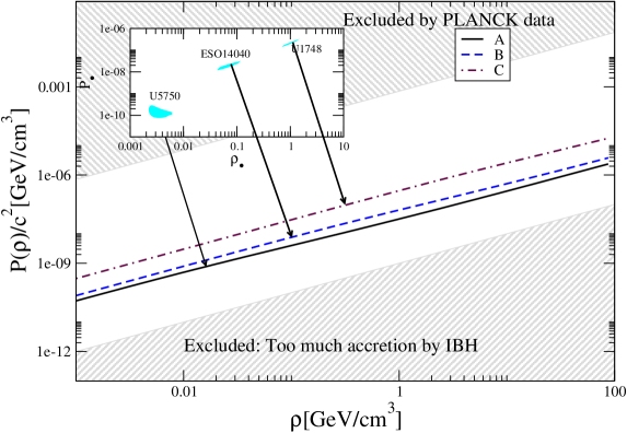
Figure 2: By fixing ($\bar{\rho}_{\bullet},\bar{p}_{\bullet}$) with the central values of the fit in equation (1) three different EoS $\bar{P}(\bar{\rho})$ are obtained. Those EoS are plotted and compared its behavior with current exclusion areas obtained by analysing the CMB anisotropies Xu [2013] and dark matter accretion by Intermediate Mass Black Holes Pepe [2011], Lora-Clavijo [2014]. Inset plot: Contours at 90% C.L. in the ($\bar{\rho}_{\bullet},\bar{p}_{\bullet}$) plane that fits the rotational curve velocities of the galaxies listed in Table 1.

In Fig. 2, the resulting EoS for each pair ($\bar{\rho}_{\bullet}$,$\bar{p}_{\bullet}$) are plotted. The inset plot shows the allowed region in the space ($\bar{\rho}_{\bullet}$,$\bar{p}_{\bullet}$) that fits the rotational velocity data of the mentioned galaxies in Table 1 at 90% of C.L. These three galaxies cover most of the relevant region that fits most of the 20 galaxies studied in Barranco [2013]. The resulting dark matter EoS that we explore are within the allowed region that is not excluded neither by analysis done using cosmological data [Xu, 2013] nor by studies of accretion of dark matter by Intermediate Mass Black Holes [Pepe, 2011, Lora-Clavijo, 2014].

3.1 EOS with fixed parameters

In the present work we interpret equation 1 in two ways. First, in this section, we consider that $\bar{\rho}_{\bullet}$ and $\bar{p}_{\bullet}$ are constants valid for all possible dark matter halos, therefore there is a unique EoS for dark matter where the only relevant variables are the density and pressure. Once we have such an EoS, we integrate the TOV equations, varying the central pressure $\bar{p}_{0}$, obtaining a family of dark matter objects.

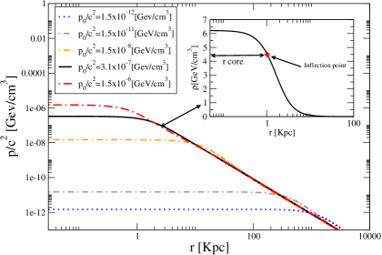
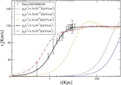
Figure 3: Left panel: Radial pressure profiles obtained as solutions of the TOV equations with dark matter EoS labeled as EoS B in Table 1. Each curve corresponds to a different initial value for $\bar{p}_{0}$. Inset plot shows the equivalent radial density profile $\rho(r)$ obtained by mapping the pressure profiles via equation 1 for the particular case where $\bar{p}_{0}=\bar{p}_{\bullet}$. The red point corresponds to the point where the density profile has an inflection point and we define the core radius of the configuration as the radius where this inflexion point occurs. Right panel: The rotational velocity profile for different halos (different initial values of $P_{0})$ within one family of solutions. It can be observed that from all those configurations only the configuration where $\bar{p}_{0}=\bar{p}_{\bullet}$ can fit the observed rotational velocities for the galaxy ESO2060140.

With compact objects obtained from the EoS through the TOV equations, an important feature is the M-R (mass-radius) diagram. This diagram gives an idea of the typical sizes of possible objects and a criterion for stability of the configurations. For barotropic EoS, and also for the EoS 21, there is the problem of defining the radius of the object, since the pressure and density never become zero, and the mass is divergent. Specifically, for a barotropic EoS the pressure decreases quadratically with $r$, with the density decreasing also quadratically, and therefore the mass increasing linearly. As the pressure never becomes zero there is not a clear way of defining the size of the object. As we have mentioned earlier, for $\bar{p}\ll 1$ the EoS given by equation 21 has a barotropic limit, which is consistent with the feature of flat rotation curve profile of the galaxies for large values of $\bar{r}$ and can not be avoided in the present setting. To overcome this problem we consider the boundary of the halo to be located where the density of dark matter becomes the density of dark matter in between galaxies. That is, we consider the radius at which it is no longer possible to distinguish between the halo and the dark matter background. For this, we take the value of [Aghanim, 2018]:

$$\rho_{m}=1.2\times 10^{-6}\,GeV/cm^{3},$$ (22)

which in our dimensionless variables reads as

$$\bar{\rho}_{m}=1.3\times 10^{-8}.$$ (23)

Therefore, we consider the radius $R$ and mass $M$ of the dark matter object as the radius and mass where the dark matter density is equal to $\rho_{m}$.

The velocity profile given by equation 16 has been proposed because it has constant rotational velocities for $\bar{r}\gg 1$ and for cored galaxies. Thus, it is natural to expect that the resulting density profile from the solution of the TOV system with EoS given by equation 1 have a core. We consider the ”core” of the object as the radius where the density profile has an inflection point, and denote such radius as $R_{core}$ and the corresponding mass as $M_{core}$.

Table 2: Maximum mass for the dark matter halos and related parameters.

EoS	$M\,[10^{10}M_{\odot}]$	$M_{core}\,[10^{10}M_{\odot}]$	$R\,[kpc]$	$R_{core}\,[kpc]$	$\bar{\rho}_{0}$	$\bar{p}_{0}$
A	$756$	$45.1$	$2851$	$668$	$1.86\times 10^{-7}$	$9.7\times 10^{-15}$
B	$1437$	$86$	$3531$	$828$	$1.86\times 10^{-7}$	$1.49\times 10^{-14}$
C	$11242$	$672$	$7009$	$1644$	$1.86\times 10^{-7}$	$5.9\times 10^{-14}$

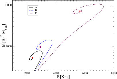
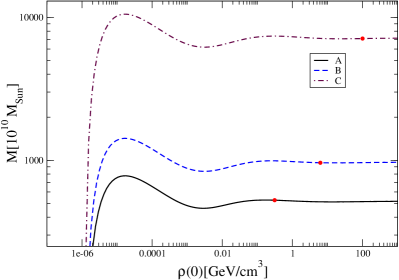
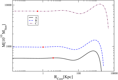
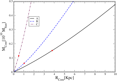
Figure 4: Main properties of the dark matter halos obtained with the A,B,C EoS. From left to right and from up to down: The total mass $M$ as a function of the radius of the halo $R$. The total mass $M$ as a function of the central density $\rho(0)$. The total mass $M$ as a function of the core radius $R_{core}$ and finally, the mass of the core as a function of the core radius. With a red point the configurations that fit the observed rotational curves of the galaxies enumerated in Table 1 are shown. In all cases, the red points are in the unstable branch.

To perform the numerical integration of equations 10-11 we use the Runge-Kutta-Felhberg (4,5) algorithm already implemented in SageMath [SageMath, ]. Due to the system of ODEs being formally singular at $\bar{r}=0$, we use the Taylor expansions 13-14 to transport the initial conditions to the first point of the integration grid. We use a non-uniform grid, due to the relatively fast change of variables close to $\bar{r}=0$ with respect to the regions far away from the center. The $k$$-th$ point of the integration grid is

$$\bar{r}_{k}=\bar{r}_{n}\left(\frac{k}{n}\right)^{1.2},\quad k=1,\ldots,n,$$ (24)

being $n$ the number of points on the grid, and $\bar{r}_{n}$ the upper limit for the integration. We use $n=10^{5}$. Examples of the solutions can be seen in Figure 3. The left panel shows radial pressure profiles obtained as solutions of the TOV equations with the dark matter EoS labeled as EoS B in Table 1. Each curve corresponds to a different initial value for $\bar{p}_{0}$. Black solid line corresponds to the solution with $\bar{p}_{0}=\bar{p}_{\bullet}$. The inset plot shows the equivalent radial density profile $\rho(r)$ obtained by mapping the pressure profile via equation 1 for this particular case where $\bar{p}_{0}=\bar{p}_{\bullet}$. The red diamond corresponds to the point where the density profile has an inflexion point and we define the core radius of the configuration as the radius where this inflection point occurs. Besides the radial pressure profile $\bar{p}(\bar{r})$, the mass profile $\bar{m}(\bar{r})$ is obtained as well as solution of the TOV system. Thus the rotational velocity profile can be directly computed by $v_{t}=\sqrt{\frac{Gm(r)}{r}}\,.$

The right panel of Fig. 3 shows the rotational velocity profiles for the different halos that corresponds to the pressure profiles from the left panel. It should be noted that although the EoS was obtained from the PSS velocity profile, in the family of solutions, the only object that fits this profile is the one that has exactly the values $\bar{\rho}_{0}=\bar{\rho}_{\bullet}$ and $\bar{p}_{0}=\bar{p}_{\bullet}$. To make this point explicit, in Figure 3 we have plotted the velocity profiles of five halos in the same family. We have used a logarithmic scale on the axis of abscissas to make the differences in the profiles more obvious, remembering that the only PSS profile is the one with $\bar{p}_{0}=3.8\times 10^{-9}$.

In Figure 4, the diagrams for mass vs radius, mass vs central density, mass vs core radius and core mass vs core radius, respectively, are presented, using the parameters ($\bar{\rho}_{\bullet},\bar{p}_{\bullet}$) shown in Table 1 for the EoS obtained from the galaxies U5750, ESO2060140 and U11748, now labeled as EoS A,B and C. We see that for the three pairs of $(\bar{\rho}_{\bullet},\bar{p}_{\bullet})$ here considered, the results are qualitatively the same. The mass has a maximum, indicating the existence of a stable branch and an unstable branch. Here we use the criteria that a static object of perfect fluid can only pass from stability to instability with respect to some particular radial normal mode at a value of the central density where the mass is an extreme [Weinberg, 1972]. The maximum mass, and the corresponding radius, core radius and core mass are summarized in Table 2. It is of interest to note that the value of $\bar{\rho}_{0}$ for the maximum mass coincides to the third digit for the three families of galaxies. It seems to indicate that the deciding factor for the stability is the central density; objects with lower central densities being stable, while objects with higher central densities being unstable. In Figure 4, the halos obtained with the value $\bar{p}_{0}=\bar{p}_{\bullet}$, that are the only ones that fit the corresponding observed rotational velocities of the galaxies, are depicted with a red dot, and in all cases they are definitely unstable. Similarly, in Figure 3 the profile for $\bar{\rho}_{0}\leq 1.86\times 10^{-7}$ correspond to a stable halo object while the others are unstable.

Figure 4 summarizes the global general properties of dark matter halos that can be obtained with the EoS derived from the PSS velocity profile. The core radius is an important one. Note that the core radius for stable configurations is bigger than 100 Kpc. Thus, the stable configurations are unable to fit the observed rotational curves, as they demand cores of the order of a few kiloparsecs. This issue can be seen graphically on the right panel of Figure 3. Following with the analysis of the core radius of the resulting self-gravitating objects that models our dark matter halos, in Figure 5 we have plotted the core radius as a function of the central density. Here again, the red dots indicate the values that best fit the rotational curves of galaxies shown in Table 1. Furthermore, the solid red line shown in Figure 5 corresponds to the observational evidence that the central surface density, defined as the product of the central density times the core radius, of galaxy dark matter halos, is nearly constant and independent of galaxy luminosity [Donato, 2009, Gentile, 2009]. Observe that in general, A,B and C EoS studied in this work do not follow this universal relation of constant surface density. It is worth noting that the best fit point for the galaxy ESO2060140 lies near the red solid line, this motivates us to explore another possible set of EoS as equation 1.

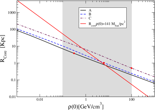
Figure 5: $R_{core}$ as a function of $\rho(0)$ for the EoS with fixed parameters ($\bar{p}_{\bullet},\bar{\rho}_{\bullet}$) studied in this work. The values of the core radius of the halos that fit the observed rotational velocities are of the order of few kiloparsecs, while the core radius of the stable configurations, with $\bar{\rho}_{0}<1.86\times 10^{-7}$, are of the order of a thousand kiloparsecs. The red solid line corresponds to the relation $R_{core}\rho_{0}=141M_{\odot}/$pc² found in Donato [2009], Gentile [2009].

3.2 Constant ($\rho_{0}R_{core}$)

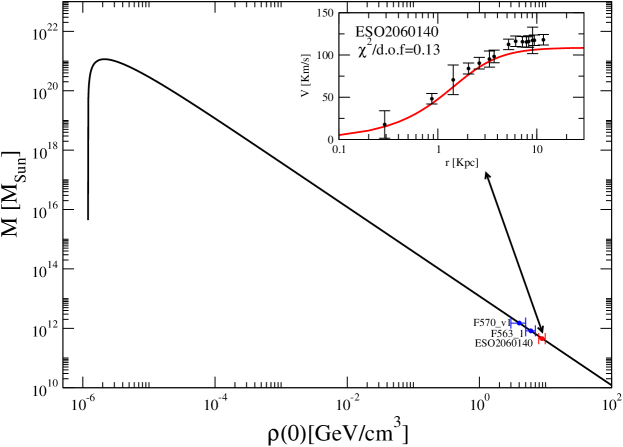
Figure 6: Plot of $\bar{m}_{m}(\bar{\rho}_{0})$ with constant $\bar{p}_{\bullet}$ and variable $\bar{\rho}_{0}=\bar{\rho}_{\bullet}$. The maximum mass is reached for $\bar{\rho}_{0,crit}=2.7\times 10^{-8}$; all configurations to the right are unstable. The value of $\bar{\rho}_{0}$ needed to fit the rotational curve of ESO2060140 is bigger that this value, thus the configuration that fits the data are in the unstable branch.

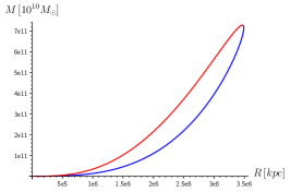
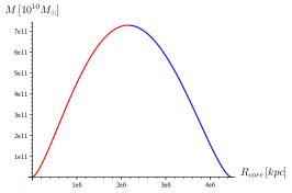
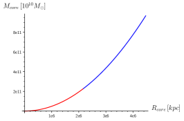
Figure 7: $M-R$, $M-R_{core}$ and $M_{core}-R_{core}$ diagrams for the EoS with constant $\bar{p}_{0}$.

Our previous results reveal a fundamental problem when the EoS given by equation 1 is used to model dark matter halos: the halo that fit the rotational curve belongs to the unstable branch of possible configurations. This could be an effect of the particular (and arbitrary) selection of the sets of parameters ($\bar{\rho}_{\bullet},\bar{p}_{\bullet}$) that we have done. In this section, we interpret the EoS in a different way. We assume that all galaxies follow the PSS rotational velocity profile, which gives rise to the dark matter EoS 1, but they do not have the same $\bar{\rho}_{\bullet}$. Instead of that, following the work Donato [2009], Gentile [2009], we consider that the product $\rho_{0}~{}R_{core}$ has the constant value

$$\rho_{0}~{}R_{core}=141^{+82}_{-52}\,M_{\odot}/pc^{2}.$$ (25)

The core radius is where the density profile has an inflection point, and from 18,

$$\bar{r}_{core}=\sqrt{\frac{2\sqrt{34}-11}{3}}a=\sqrt{2\sqrt{34}-11}\sqrt{\frac{\bar{p}_{\bullet}}{G_{\star}}}\frac{1}{\bar{\rho}_{0}},$$ (26)

which together with 25 implies

$$\bar{p}_{0}=\bar{p}_{\bullet}=\frac{G_{\star}(\bar{\rho}_{0}~{}\bar{r}_{core})^{2}}{2\sqrt{34}-11}=2.5\times 10^{-9}.$$ (27)

Now, we interpret 1 in the following way. The parameter $\bar{p}_{\bullet}$ in 1 is a constant for all galaxies, having the value 27. The parameter $\bar{\rho}_{\bullet}$ is both the corresponding parameter in 1 and the central density of the galaxies $\bar{\rho}_{0}$, and it is not a constant for different galaxies. Therefore, we have a family of dark matter objects, parameterized by $\bar{\rho}_{0}$, each galaxy with an EoS with its own set of parameters, being $\bar{p}_{\bullet}$ a constant. Although having a different EoS for each galaxy may seem like the model loses its value, the interpretation is not that each galaxy possess a different type of dark matter. Instead of that, we consider that there is another parameter, the simplest one being the temperature, which has not been considered here. In this sense, having EoSs with different parameters amount to having galaxies with different temperature profiles. The interpretation is the same as with the classical Eddington model for stars made of an ideal gas, where the EoS is that of an ideal gas, but the temperature profile is supposed to be such that the pressure contribution from the gas has a constant ratio with respect to the radiation pressure. In this way, the equations for $p$ and $m$ can be integrated without explicitly considering the temperature, and each star has a particular EoS in the form $\rho(p)$.

With this interpretation in mind, there is only one family of solutions with only one free parameter: the central density $\bar{\rho}_{0}$. The values of $R$, $R_{core}$, $M$ and $M_{core}$ have the same meaning as before, but now they can be obtained analytically as functions of central density $\bar{\rho}_{0}$, from 17 and 18. Then, in terms of the dimensionless quantities, we have the mass of the core:

$$\bar{m}_{core}=\bar{m}(\bar{r}_{core})=\frac{3(2\sqrt{34}-11)^{\frac{3}{2}}}{2(\sqrt{34}-4)}\frac{\bar{p}_{\bullet}^{\frac{3}{2}}}{G_{\star}^{\frac{3}{2}}\bar{\rho}_{0}^{2}}.$$ (28)

The dark matter halo ends at the point where $\bar{\rho}$ given in equation 18 is equal to $\bar{\rho}_{m}$, and therefore the radius of the configuration is

$$\bar{r}_{m}=\sqrt{\frac{\bar{p}_{\bullet}}{2\,G_{\star}\bar{\rho}_{m}\bar{\rho}_{0}}}\sqrt{1-6\,\frac{\bar{\rho}_{m}}{\bar{\rho}_{0}}+\sqrt{1+24\,\frac{\bar{\rho}_{m}}{\bar{\rho}_{0}}}},$$ (29)

and the total mass of the halo $\bar{m}_{m}$ is obtained with $\bar{m}(\bar{r}=\bar{r}_{m})$, i.e.

$$\bar{m}_{m}=\frac{3\bar{p}_{\bullet}^{\frac{3}{2}}}{\sqrt{2}G_{\star}^{\frac{3}{2}}\sqrt{\bar{\rho}_{m}}\bar{\rho}_{0}^{\frac{3}{2}}}\frac{{\left(1-6\,\frac{\bar{\rho}_{m}}{\bar{\rho}_{0}}+\sqrt{1+24\,\frac{\bar{\rho}_{m}}{\bar{\rho}_{0}}}\right)^{\frac{3}{2}}}}{1+\sqrt{1+24\,\frac{\bar{\rho}_{m}}{\bar{\rho}_{0}}}}.$$ (30)

Equation 30 gives the mass of the halo as a function of the central density. We have plotted $\bar{m}(\rho_{0})$ in Figure 6. We see that the mass has a maximum value, which from equation 30 corresponds to the central density

$$\bar{\rho}_{0,crit}=(3\sqrt{19}-11)\bar{\rho}_{m}=2.7\times 10^{-8},$$ (31)

being the maximum mass

$$M_{crit}=\frac{3\sqrt{951029+220742\sqrt{19}}\bar{p}_{\bullet}}{12500G_{\star}^{3/2}\bar{\rho}_{m}^{2}}=7.3\times 10^{21}M_{\odot},$$ (32)

and the corresponding object radius

$$R_{crit}=\frac{232+61\sqrt{19}}{625\bar{\rho}_{m}}\sqrt{\frac{\bar{p}_{\bullet}}{2G_{\star}}}=3.5\times 10^{6}kpc.$$ (33)

Although, it is possible to obtain analytical expressions for these quantities in terms of one of the others, for instance $\bar{m}_{m}(\bar{r}_{m})$, the formulas are not very enlightening and we prefer to consider them as given parametrically through $\bar{\rho}_{0}$. For the configuration with maximum mass, the core radius is

$$R_{core,crit}=2.2\times 10^{6}kpc,$$ (34)

being the core mass

$$M_{core,crit}=2.2\times 10^{21}M_{\odot}.$$ (35)

In Figure 7, the relationship between mass, core mass, radius and core radius, are shown. The maximum mass represents, as before, the configuration that divides stable from unstable configurations. The stable branch are those objects with

$$\bar{\rho}_{0}<\bar{\rho}_{0,crit},\quad M<M_{crit},\$$ (36)

$$M_{core}>M_{core,crit},\quad R_{core}>R_{core,crit},$$ (37)

while the unstable branch is the one with

$$\bar{\rho}_{0}>\bar{\rho}_{0,crit},\quad M<M_{crit},$$ (38)

$$M_{core}<M_{core,crit},\quad R_{core}<R_{core,crit}.$$ (39)

In Figure 7, the unstable branch is indicated by the red curve, while the stable branch by the blue one.

As expected, we can fit some rotational velocities profiles with this set of configurations. The fit can be done through a $\chi^{2}$ analysis of the rotational curves measured in some Low Surface Brightness Galaxies [de Blok, 2002] and the theoretical curve obtained by equation 3.1, with the mass computed by equation 30. There is only one free parameter, $\bar{\rho}_{0}$, and thus we minimize $\chi^{2}(\bar{\rho}_{0})=\sum_{i}\frac{(v_{t}^{i}-v_{t}(\bar{\rho}_{0}))^{2}}{(\delta v_{t}^{i})^{2}}$ in order to find the best fit point. Here $v_{t}^{i}$ are the observed data and $\delta v_{t}^{i}$ are the errors in the data points reported in de Blok [2002]. The particular case of the rotational velocity data from ESO2060140 is shown as an inset plot in Figure 6. It can be seen that the fit is reasonable good ($\chi^{2}_{min}/\text{d.o.f.}=0.13$). The best fit value for this galaxy is $\bar{\rho}_{0}=8.87$ GeV/cm³, and it is plotted in Figure 6 as a red point. Thus, this dark matter halo lies on the unstable branch. Other galaxies also can be fitted by fixing $\bar{p}_{\bullet}$, as it has been explained above. For instance, the galaxies F563-1 and F570 v1, and the best fit points for those galaxies are plotted as blue points in Figure 6. One more time, those configurations are in the unstable branch.

Table 3: Gravitational energy and related parameters for the last stable configurations.

Galaxy	$M\,[10^{10}M_{\odot}]$	$R\,[\mbox{kpc}]$	Gravitational energy  $[Mc^{2}]$	Density $[gr/cm^{3}]$	Surface gravity
U5750	$756$	$2851$	$1.27\times 10^{-7}$	$5.27\times 10^{-30}$	$1.29\times 10^{-13}$
ESO2060140	$1437$	$3531$	$0.002$	$5.27\times 10^{-30}$	$1.61\times 10^{-13}$
U11748	$11242$	$7009$	$0.080$	$5.99\times 10^{-27}$	$3.47\times 10^{-11}$

4 Discussion

We have integrated the TOV system with the dark matter EoS given by equation 1. Four cases where analyzed: three family of solutions were obtained for the representative sets of parameters ($\bar{p}_{\bullet},\bar{\rho}_{\bullet}$) given in Table 1, as they cover most of the parameter space that can fit the observed rotational velocities of Low Surface Brightness Galaxies. The fourth family of solutions was obtained by fixing $\bar{p}_{\bullet}$ in order for the constancy of the surface brightness in galaxies found in Donato [2009], Gentile [2009] to be always satisfied. This last family of solutions has as free parameter the central density. The four families of dark matter halos have similar properties and one configuration in all cases is of special interest: the configuration with maximum mass. The parameters presented in table 2 represent the maximum mass and corresponding radii for our galaxy halos. The stable configurations are to the right of the maximum and the unstable ones to the left in the $M-R$ diagrams. As it is common in various mass-radius relations, for large values of the central pressure the curves start to curl. The maximum in the curves divide the stable configurations from the unstable ones. The halos that fit the rotational curve for the considered galaxies are all on the unstable branch.

In table 3 we have estimations for the gravitational energy, the density and the surface gravity of the halos of our set of three galaxies. Clearly, we found that, due to the gravitational energy being not an appreciable fraction of the rest energy, the halos are not considered relativistic objects. Even more, the mean density is low, in the order of the current density of the Universe of $9.9\times 10^{-30}$ gr/cm³, in correspondence to a flat universe. However, U11748 exhibits a higher density, about $6\times 10^{-27}$ gr/cm³, so it is able to expand openly. This happens because the stable configurations need to have a central density which is only a few times the average density of the universe. Thus the dark matter halos have radius of the order of thousand of kiloparsecs, core radius of hundred of kiloparsecs and therefore stable halos obtained through equation 1 are not good models for realistic halos that fit the rotational curve of galaxies. Finally, we see that the surface gravity of the halos is extremely low, of about $10^{-11}-10^{-13}$ cm/s². Then, we conclude, the halo system is not relativistic and the $\frac{2Gm}{c^{2}r}$ factor, that appears in the TOV equation (4), which determines the effects of General Relativity, is negligible. This is the reason why the Newtonian approximation produces the same results as the relativistic one when describing the dark matter halos in elliptical galaxies.

5 Conclusions

The rotation curves of spiral galaxies determine completely the corresponding Newtonian gravitational potential $\Phi(r)$ of the static, spherically symmetric spacetime metric. This implies that the gravitational field inside the halo is weak, of the order of $\beta^{2}$, and the temporal term of the metric is not dependent on the equation of state used to describe the dark matter component. Once a phenomenological rotational profile is proposed for a galaxy, if the dark matter is modeled as a perfect fluid, then the equation of state for dark matter is determined by the rotational velocity profile. In particular, if the rotational velocity profile predicts a flat rotation curve for large radii, as the velocity profile proposed in Persic [1996], then the resulting EoS for dark matter, given by equation 1, has a barotropic limit for $\bar{r}\gg 1$. The resulting density profile decays as the inverse square power of the radial coordinate and in consequence the density and pressure never reach zero at the boundary of the halo. Moreover, as it was mentioned in section II, the halo mass is divergent, increasing linearly in $r$. This fact implies that the invisible matter distributed in a spherical halo around spiral galaxies extend to infinity. Despite this, by defining the radius of the halo as the point where the halo density matches the average density of the Universe we can circumvent this problem. More troublesome, once the configurations that fit the observed rotational velocity curves of Low Surface Brightness Galaxies are found, they in fact are in the unstable branch of possible configurations. This shows that although it is possible to find halos that fit the observed data, those configurations demand central pressures and densities that are too high regarding hydrostatic equilibrium, and therefore will be unstable under small radial perturbations. We conclude that if the Universal Velocity profile should be valid to fit the rotational velocity curve of the galaxies and dark matter could be modeled as a perfect fluid, then one of our assumptions, e.g. hydrostatic equilibrium, spherical symmetry, or staticity of the spacetime, should not be valid.

References

- Aghanim [2018] Aghanim N. et al. [Planck], Astron. Astrophys. 641 (2020), A6 doi:10.1051/0004-6361/201833910 [arXiv:1807.06209 [astro-ph.CO]].
- Barranco [2013] Barranco J., Bernal A. and Nunez D., Mon. Not. Roy. Astron. Soc. 449 (2015) no.1, 403-413 doi:10.1093/mnras/stv302 [arXiv:1301.6785 [astro-ph.CO]].
- Boylan-Kolchin [2011] Boylan-Kolchin M., Bullock J. S. and Kaplinghat M., Mon. Not. Roy. Astron. Soc. 415 (2011), L40 doi:10.1111/j.1745-3933.2011.01074.x [arXiv:1103.0007 [astro-ph.CO]].
- Calabrese [2009] Calabrese E., Migliaccio M., Pagano L., De Troia G., Melchiorri A. and Natoli P., Phys. Rev. D 80 (2009), 063539 doi:10.1103/PhysRevD.80.063539
- de Blok [2002] de Blok W. J. G., Bosma A., Astronomy and Astrophysics, 385 (2002), 816–846 doi: 10.1051/0004-6361:20020080
- Donato [2009] Donato F., et. al., Mon. Not. Roy. Astron. Soc. 397 (2009), 1169-1176 do: 10.1111/j.1365-2966.2009.15004.x [arXiv:0904.4054 [astro-ph.CO]].
- Flores [1994] Flores R. A. and Primack J. R. , Astrophys. J. Lett. 427 (1994), L1-4 doi:10.1086/187350 [arXiv:astro-ph/9402004 [astro-ph]].
- Gentile [2009] Gentile G. , Famaey B. , Zhao H. and Salucci P., Nature 461 (2009), 627 doi:10.1038/nature08437 [arXiv:0909.5203 [astro-ph.CO]].
- Gong [2020] Gong X., Tang M. and Xu Z., doi:10.1088/1674-1137/ac0f73 [arXiv:2007.02583 [astro-ph.GA]].
- Ibata [2000] Ibata R., Lewis G. F., Irwin M., Totten E. and Quinn T. R., Astrophys. J. 551 (2001), 294-311 doi:10.1086/320060 [arXiv:astro-ph/0004011 [astro-ph]].
- Karukes [2015] Karukes E. V., Salucci P. and Gentile G., Astron. Astrophys. 578 (2015), A13 doi:10.1051/0004-6361/201425339 [arXiv:1503.04049 [astro-ph.GA]].
- Klypin [1999] Klypin A. A., Kravtsov A. V., Valenzuela O. and Prada F., Astrophys. J. 522 (1999), 82-92 doi:10.1086/307643 [arXiv:astro-ph/9901240 [astro-ph]].
- Kopp [2018] Kopp M., Skordis C., Thomas D. B. and Ilić S., Phys. Rev. Lett. 120 (2018) no.22, 221102 doi:10.1103/PhysRevLett.120.221102 [arXiv:1802.09541 [astro-ph.CO]].
- Lora-Clavijo [2014] Lora-Clavijo F. D., Garcia-Linares M. and Guzman F. S., Mon. Not. Roy. Astron. Soc. 443 (2014) no.3, 2242-2251 doi:10.1093/mnras/stu1289 [arXiv:1406.7233 [astro-ph.GA]].
- Moore [1999] Moore B., Ghigna S., Governato F., Lake G., Quinn T. R., Stadel J. and Tozzi P., Astrophys. J. Lett. 524 (1999), L19-L22 doi:10.1086/312287 [arXiv:astro-ph/9907411 [astro-ph]].
- Muller [2004] Muller C. M., Phys. Rev. D 71 (2005), 047302 doi:10.1103/PhysRevD.71.047302 [arXiv:astro-ph/0410621 [astro-ph]].
- Nunez [2010] Nunez D., Gonzalez-Morales A. X., Cervantes-Cota J. L. and Matos T., Phys. Rev. D 82 (2010), 024025 doi:10.1103/PhysRevD.82.024025 [arXiv:1006.4875 [astro-ph.GA]].
- Oppenheimer [1939] Oppenheimer J. R., Volkov G. M., 1939, Phys. Rev., 55, 374
- Pepe [2011] Pepe C., Pellizza L. J. and Romero G. E., Mon. Not. Roy. Astron. Soc. 420 (2012), 3298-3302 doi:10.1111/j.1365-2966.2011.20252.x [arXiv:1111.5605 [astro-ph.HE]].
- Perivolaropoulos [2021] Perivolaropoulos L. and Skara F., [arXiv:2105.05208 [astro-ph.CO]].
- Persic [1996] Persic M. et al., 1996, Mon. Not. R. Astron. Soc. 281, 27-47.
- Rahaman [2011] Rahaman F., Nandi K. K., Bhadra A., Kalam M. and Chakraborty K., Phys. Lett. B 694 (2011), 10-15 doi:10.1016/j.physletb.2010.09.038 [arXiv:1009.3572 [gr-qc]].
- [23] SageMath, the Sage Mathematics Software System (Version x.y.z), The Sage Developers, http://www.sagemath.org.
- Silbar [2004] Silbar R., Reddy S., (2004). Neutron stars for undergraduates.
- Serra [2011] Serra A.L. and Romero M. J. d., Mon. Not. Roy. Astron. Soc. 415 (2011), 74 doi:10.1111/j.1745-3933.2011.01082.x [arXiv:1103.5465 [gr-qc]].
- Sofue [2000] Sofue Y. and Rubin V., Ann. Rev. Astron. Astrophys. 39 (2001), 137-174 doi:10.1146/annurev.astro.39.1.137 [arXiv:astro-ph/0010594 [astro-ph]].
- Spergel [1999] Spergel D. N. and Steinhardt P. J., Phys. Rev. Lett. 84 (2000), 3760-3763 doi:10.1103/PhysRevLett.84.3760 [arXiv:astro-ph/9909386 [astro-ph]].
- Tolman [1939] Tolman R. C., 1939, Phys. Rev., 55, 364
- Xu [2013] Xu L. and Chang Y., Phys. Rev. D 88 (2013), 127301 doi:10.1103/PhysRevD.88.127301 [arXiv:1310.1532 [astro-ph.CO]].
- Yang [2015] Yang L., Yang W. Q. and Xu L. X., Chin. Phys. Lett. 32 (2015) no.5, 059801 doi:10.1088/0256-307X/32/5/059801
- Weinberg [2015] Weinberg D. H., Bullock J. S., Governato F., Kuzio de Naray R. and Peter A. H. G., Proc. Nat. Acad. Sci. 112 (2015), 12249-12255 doi:10.1073/pnas.1308716112 [arXiv:1306.0913 [astro-ph.CO]].
- Weinberg [1972] Weinberg s., Gravitation and Cosmology: Principles and Applications of the General Theory of Relativity”, Wiley, New York (1972).
- Zavlin [1995] Zavlin V. E. et al., Astronomy Letters, 21, 149 (1995).