Faster Deep Reinforcement Learning with
Slower Online Network

Abstract

Deep reinforcement learning algorithms often use two networks for value function optimization: an online network, and a target network that tracks the online network with some delay. Using two separate networks enables the agent to hedge against issues that arise when performing bootstrapping. In this paper we endow two popular deep reinforcement learning algorithms, namely DQN and Rainbow, with updates that incentivize the online network to remain in the proximity of the target network. This improves the robustness of deep reinforcement learning in presence of noisy updates. The resultant agents, called DQN Pro and Rainbow Pro, exhibit significant performance improvements over their original counterparts on the Atari benchmark demonstrating the effectiveness of this simple idea in deep reinforcement learning. The code for our paper is available here: Github.com/amazon-research/fast-rl-with-slow-updates.

1 Introduction

An important competency of reinforcement-learning (RL) agents is learning in environments with large state spaces like those found in robotics (Kober et al., 2013), dialog systems (Williams et al., 2017), and games (Tesauro, 1994; Silver et al., 2017). Recent breakthroughs in deep RL have demonstrated that simple approaches such as Q-learning (Watkins & Dayan, 1992) can surpass human-level performance in challenging environments when equipped with deep neural networks for function approximation (Mnih et al., 2015).

Two components of a gradient-based deep RL agent are its objective function and optimization procedure. The optimization procedure takes estimates of the gradient of the objective with respect to network parameters and updates the parameters accordingly. In DQN (Mnih et al., 2015), for example, the objective function is the empirical expectation of the temporal difference (TD) error (Sutton, 1988) on a buffered set of environmental interactions (Lin, 1992), and variants of stochastic gradient descent are employed to best minimize this objective function.

A fundamental difficulty in this context stems from the use of bootstrapping. Here, bootstrapping refers to the dependence of the target of updates on the parameters of the neural network, which is itself continuously updated during training. Employing bootstrapping in RL stands in contrast to supervised-learning techniques and Monte-Carlo RL (Sutton & Barto, 2018), where the target of our gradient updates does not depend on the parameters of the neural network.

Mnih et al. (2015) proposed a simple approach to hedging against issues that arise when using bootstrapping, namely to use a target network in value-function optimization. The target network is updated periodically, and tracks the online network with some delay. While this modification constituted a major step towards combating misbehavior in Q-learning (Lee & He, 2019; Kim et al., 2019; Zhang et al., 2021), optimization instability is still prevalent (van Hasselt et al., 2018).

Our primary contribution is to endow DQN and Rainbow (Hessel et al., 2018) with a term that ensures the parameters of the online-network component remain in the proximity of the parameters of the target network. Our theoretical and empirical results show that our simple proximal updates can remarkably increase robustness to noise without incurring additional computational or memory costs. In particular, we present comprehensive experiments on the Atari benchmark (Bellemare et al., 2013) where proximal updates yield significant improvements, thus revealing the benefits of using this simple technique for deep RL.

2 Background and Notation

RL is the study of the interaction between an environment and an agent that learns to maximize reward through experience. The Markov Decision Process (Puterman, 1994), or MDP, is used to mathematically define the RL problem. An MDP is specified by the tuple $\langle\mathcal{S,A,R,P,\gamma}\rangle$, where $\mathcal{S}$ is the set of states and $\mathcal{A}$ is the set of actions. The functions $\mathcal{R:S\times A\rightarrow}\ \mathbb{R}$ and $\mathcal{P:S\times A\times S\rightarrow}\ [0,1]$ denote the reward and transition dynamics of the MDP. Finally, a discounting factor $\gamma$ is used to formalize the intuition that short-term rewards are more valuable than those received later.

The goal in the RL problem is to learn a policy, a mapping from states to a probability distribution over actions, ${\pi:\mathcal{S}\rightarrow\mathcal{P}(\mathcal{A})}$, that obtains high sums of future discounted rewards. An important concept in RL is the state value function. Formally, it denotes the expected discounted sum of future rewards when committing to a policy $\pi$ in a state $s$: $v^{\pi}(s)\vcentcolon=\mathbb{E}\big{[}\sum_{t=0}^{\infty}\gamma^{t}R_{t}\big{|}S_{0}=s,\pi\big{]}\ .$ We define the Bellman operator $\mathcal{T^{\pi}}$ as follows:

$$\big{[}\mathcal{T^{\pi}}v\big{]}(s):=\!\sum_{a\in\mathcal{A}}\pi(a\mid s)\big{(}\mathcal{R}(s,a)+\!\sum_{s^{\prime}\in\mathcal{S}}\!\gamma\ \mathcal{P}(s,a,s^{\prime})v(s^{\prime})\big{)}\ ,$$

which we can write compactly as: $\mathcal{T}^{\pi}v\vcentcolon=R^{\pi}+\gamma P^{\pi}v\ ,$ where $\big{[}R^{\pi}\big{]}(s)=\sum_{a\in\mathcal{A}}\pi(a|s)\mathcal{R}(s,a)$ and $\big{[}P^{\pi}v\big{]}(s)=\sum_{a\in\mathcal{A}}\pi(a\mid s)\sum_{s^{\prime}\in\mathcal{S}}\!\mathcal{P}(s,a,s^{\prime})v(s^{\prime})$. We also denote: $(\mathcal{T}^{\pi})^{n}v\vcentcolon=\underbrace{\mathcal{T}^{\pi}\cdots\mathcal{T}^{\pi}}_{n\ \textrm{compositions}}v\ .$ Notice that $v^{\pi}$ is the unique fixed-point of $(\mathcal{T}^{\pi})^{n}$ for all natural numbers $n$, meaning that $v^{\pi}=(\mathcal{T}^{\pi})^{n}v^{\pi}\$, for all $n$. Define $v^{\star}$ as the optimal value of a state, namely: ${v^{\star}(s)\vcentcolon=\max_{\pi}v^{\pi}(s)}$, and $\pi^{\star}$ as a policy that achieves $v^{\star}(s)$ for all states. We define the Bellman Optimality Operator $\mathcal{T^{\star}}$:

$$\big{[}\mathcal{T^{\star}}v\big{]}(s):=\!\max_{a\in\mathcal{A}}\mathcal{R}(s,a)+\!\sum_{s^{\prime}\in\mathcal{S}}\!\gamma\ \mathcal{P}(s,a,s^{\prime})v(s^{\prime})\ ,$$

whose fixed point is $v^{\star}$. These operators are at the heart of many planning and RL algorithms including Value Iteration (Bellman, 1957) and Policy Iteration (Howard, 1960).

3 Proximal Bellman Operator

In this section, we introduce a new class of Bellman operators that ensure that the next iterate in planning and RL remain in the vicinity of the previous iterate. To this end, we define the Bregman Divergence generated by a convex function $f$:

$$D_{f}(v^{\prime},v)\vcentcolon=f(v^{\prime})-f(v)-\langle\nabla f(v),v^{\prime}-v\rangle\ .$$

Examples include the $l_{p}$ norm generated by $f(v)=\frac{1}{2}\left\lVert v\right\rVert_{p}^{2}$ and the Mahalanobis Distance generated by $f(v)=\frac{1}{2}\langle v,Qv\rangle$ for a positive semi-definite matrix $Q$.

We now define the Proximal Bellman Operator $(\mathcal{T}^{\pi}_{c,f})^{n}$:

$$(\mathcal{T}^{\pi}_{c,f})^{n}v\vcentcolon=\arg\min_{v^{\prime}}||v^{\prime}-(\mathcal{T}^{\pi})^{n}v||^{2}_{2}+\frac{1}{c}D_{f}(v^{\prime},v)\ ,$$ (1)

where $c\in(0,\infty)$. Intuitively, this operator encourages the next iterate to be in the proximity of the previous iterate, while also having a small difference relative to the point recommended by the original Bellman Operator. The parameter $c$ could, therefore, be thought of as a knob that controls the degree of gravitation towards the previous iterate.

Our goal is to understand the behavior of Proximal Bellman Operator when used in conjunction with the Modified Policy Iteration (MPI) algorithm (Puterman, 1994; Scherrer et al., 2015). Define $\mathcal{G}v$ as the greedy policy with respect to $v$. At a certain iteration $k$, Proximal Modified Policy Iteration (PMPI) proceeds as follows:

$$\pi_{k} \leftarrow \mathcal{G}v_{k-1}\ ,$$ (2)

$$v_{k} \leftarrow (\mathcal{T}^{\pi_{k}}_{c,f})^{n}v_{k-1}\ .$$ (3)

The pair of updates above generalize existing algorithms. Notably, with $c\rightarrow\infty$ and general $n$ we get MPI, with $c\rightarrow\infty$ and $n=1$ the algorithm reduces to Value Iteration, and with $c\rightarrow\infty$ and $n=\infty$ we have a reduction to Policy Iteration. For finite $c$, the two extremes of $n$, namely $n=1$ and $n=\infty$, could be thought of as the proximal versions of Value Iteration and Policy Iteration, respectively.

To analyze this approach, it is first natural to ask if each iteration of PMPI could be thought of as a contraction so we can get sound and convergent behavior in planning and learning. For $n>1$, Scherrer et al. (2015) constructed a contrived MDP demonstrating that one iteration of MPI can unfortunately expand. As PMPI is just a generalization of MPI, the same example from Scherrer et al. (2015) shows that PMPI can expand. In the case of $n=1$, we can rewrite the pair of equations (2) and (3) in a single update as follows: $v_{k}\leftarrow\mathcal{T}^{\star}_{c,f}v_{k-1}\ .$ When $c\rightarrow\infty$, standard proofs can be employed to show that the operator is a contraction (Littman & Szepesvári, 1996). We now show that $\mathcal{T}^{\star}_{c,f}$ is a contraction for finite values of $c$. See our appendix for proofs.

Theorem 1.

The Proximal Bellman Optimality Operator $\mathcal{T}^{\star}_{c,f}$ is a contraction with fixed point $v^{\star}$.

Therefore, we get convergent behavior when using $\mathcal{T}^{\star}_{c,f}$ in planning and RL. The addition of the proximal term is fortunately not changing the fixed point, thus not negatively affecting the final solution. This could be thought of as a form of regularization that vanishes in the limit; the algorithm converges to $v^{\star}$ even without decaying $1/c$.

Going back to the general $n\geq 1$ case, we cannot show contraction, but following previous work (Bertsekas & Tsitsiklis, 1996; Scherrer et al., 2015), we study error propagation in PMPI in presence of additive noise where we get a noisy sample of the original Bellman Operator $(\mathcal{T}^{\pi_{k}})^{n}v_{k-1}+\epsilon_{k}$. The noise can stem from a variety of reasons, such as approximation or estimation error. For simplicity, we restrict the analysis to $D_{f}(v^{\prime},v)=||v^{\prime}-v||^{2}_{2}$, so we rewrite update (3) as:

$$v_{k}\leftarrow\arg\min_{v^{\prime}}||v^{\prime}-\big{(}(\mathcal{T}^{\pi_{k}})^{n}v_{k-1}+\epsilon_{k}\big{)}||^{2}_{2}+\frac{1}{c}\left\lVert v^{\prime}-v_{k-1}\right\rVert_{2}^{2}$$

which can further be simplified to:

$$v_{k}\leftarrow\underbrace{(1-\beta)(\mathcal{T}^{\pi_{k}})^{n}v_{k-1}+\beta v_{k-1}}_{:=(\mathcal{T}^{\pi_{k}}_{\beta})^{n}v_{k-1}}+(1-\beta)\epsilon_{k},$$

where $\beta=\frac{1}{1+c}$. This operator is a generalization of the operator proposed by Smirnova & Dohmatob (2020) who focused on the case of $n=1$. To build some intuition, notice that the update is multiplying error $\epsilon_{k}$ by a term that is smaller than one, thus better hedging against large noise. While the update may slow progress when there is no noise, it is entirely conceivable that for large enough values of $\epsilon_{k}$, it is better to use non-zero $\beta$ values. In the following theorem we formalize this intuition. Our result leans on the theory provided by Scherrer et al. (2015) and could be thought of as a generalization of their theorem for non-zero $\beta$ values.

Theorem 2.

Consider the PMPI algorithm specified by:

$$\pi_{k} \leftarrow \mathcal{G}_{\epsilon^{\prime}_{k}}v_{k-1}\ ,$$ (4)

$$v_{k} \leftarrow (\mathcal{T}^{\pi_{k}}_{\beta})^{n}v_{k-1}+(1-\beta)\epsilon_{k}\ .$$ (5)

Define the Bellman residual $b_{k}\vcentcolon=v_{k}-\mathcal{T}^{\pi_{k+1}}v_{k}$, and error terms $x_{k}:=(I-\gamma P^{\pi_{k}})\epsilon_{k}$ and $y_{k}:=\gamma P^{\pi^{*}}\epsilon_{k}$. After $k$ steps:

$$v^{*}-v^{\pi_{k}}=\underbrace{v^{\pi^{*}}-(\mathcal{T}^{\pi_{k+1}}_{\beta})^{n}v_{k}}_{d_{k}}+\underbrace{(\mathcal{T}^{\pi_{k+1}}_{\beta})^{n}v_{k}-v_{\pi_{k}}}_{s_{k}}$$

• where $d_{k}\leq\gamma P^{\pi^{*}}d_{k-1}-\big{(}(1-\beta)y_{k-1}+\beta b_{k-1}\big{)}+(1-\beta)\sum_{j=1}^{n-1}(\gamma P^{\pi_{k}})^{j}b_{k-1}+\epsilon^{\prime}_{k}$

• $s_{k}\leq\big{(}(1-\beta)(\gamma P^{\pi_{k}})^{n}+\beta I\big{)}(I-\gamma P^{\pi_{k}})^{-1}b_{k-1}$

• $b_{k}\leq\big{(}(1-\beta)(\gamma P^{\pi_{k}})^{n}+\beta I\big{)}b_{k-1}+(1-\beta)x_{k}+\epsilon^{\prime}_{k+1}$

The bound provides intuition as to how the proximal Bellman Operator can accelerate convergence in the presence of high noise. For simplicity, we will only analyze the effect of the $\epsilon$ noise term, and ignore the $\epsilon^{\prime}$ term. We first look at the Bellman residual, $b_{k}$. Given the Bellman residual in iteration $k-1$, $b_{k-1}$, the only influence of the noise term $\epsilon_{k}$ on $b_{k}$ is through the $(1-\beta)x_{k}$, term, and we see that $b_{k}$ decreases linearly with larger $\beta$.

The analysis of $s_{k}$ is slightly more involved but follows similar logic. The bound for $s_{k}$ can be decomposed into a term proportional to $b_{k-1}$ and a term proportional to $\beta b_{k-1}$, where both are multiplied with positive semi-definite matrices. Since $b_{k-1}$ itself linearly decreases with $\beta$, we conclude that larger $\beta$ decreases the bound quadratically.

The effect of $\beta$ on the bound for $d_{k}$ is more complex. The terms $\beta y_{k-1}$ and $\sum_{j=1}^{n-1}(\gamma P^{\pi_{k}})^{j}b_{k-1}$ introduce a linear decrease of the bound on $d_{k}$ with $\beta$, while the term $\beta(I-\sum_{j=1}^{n-1}(\gamma P^{\pi_{k}})^{j})b_{k-1}$ introduces a quadratic dependence whose curvature depends on $I-\sum_{j=1}^{n-1}(\gamma P_{\pi_{k}})^{j}$. This complex dependence on $\beta$ highlights the trade-off between noise reduction and magnitude of updates. To understand this trade-off better, we examine two extreme cases for the magnitude on the noise. When the noise is very large, we may set $\beta=1$, equivalent to an infinitely strong proximal term. It is easy to see that for $\beta=1$, the values of $d_{k}$ and $s_{k}$ remain unchanged, which is preferable to the increase they would suffer in the presence of very large noise. On the other extreme, when no noise is present, the $x_{k}$ and $y_{k}$ terms in Theorem 2 vanish, and the bounds on $d_{k}$ and $s_{k}$ can be minimized by setting $\beta=0$, i.e. without noise the proximal term should not be used and the original Bellman update performed. Intermediate noise magnitudes thus require a value of $\beta$ that balances the noise reduction and update size.

4 Deep Q-Network with Proximal Updates

We now endow DQN-style algorithms with proximal updates. Let $\langle s,a,r,s^{\prime}\rangle$ denote a buffered tuple of interaction. Define the following objective function:

$$h(\theta,w):=\widehat{\text{E}}_{\langle s,a,r,s^{\prime}\rangle}\Big{[}\big{(}r+\gamma\max_{a^{\prime}}\widehat{Q}(s^{\prime},a^{\prime};\theta)-\widehat{Q}(s,a;w)\big{)}^{2}\Big{]}\ .$$ (6)

Our proximal update is defined as follows:

$$w_{t+1}\leftarrow\arg\min_{w}h(w_{t},w)+\frac{1}{2\tilde{c}}\left\lVert w-w_{t}\right\rVert_{2}^{2}\ .$$ (7)

This algorithm closely resembles the standard proximal-point algorithm (Rockafellar, 1976; Parikh & Boyd, 2014) with the important caveat that the function $h$ is now taking two vectors as input. At each iteration, we hold the first input constant while optimizing over the second input.

In the optimization literature, the proximal-point algorithm is well-studied in contexts where an analytical solution to (7) is available. With deep learning no closed-form solution exists, so we approximately solve (7) by taking a fixed number of descent steps using stochastic gradients. Specifically, starting each iteration with $w=w_{t}$, we perform multiple $w$ updates ${w\leftarrow w-\alpha\big{(}\nabla_{2}h(w_{t},w)+\frac{1}{\tilde{c}}(w-w_{t})\big{)}}$. We end the iteration by setting $w_{t+1}\leftarrow w$. To make a connection to standard deep RL, the online weights $w$ could be thought of as the weights we maintain in the interim to solve (7) due to lack of a closed-form solution. Also, what is commonly referred to as the target network could better be thought of as just the previous iterate in the above proximal-point algorithm.

Observe that the update can be written as: $w\leftarrow\big{(}1-(\alpha/\tilde{c})\big{)}\cdot w+(\alpha/\tilde{c})\cdot w_{t}-\alpha\nabla_{2}h(w_{t},w)\ .$ Notice the intuitively appealing form: we first compute a convex combination of $w_{t}$ and $w$, based on the hyper-parameters $\alpha$ and $\tilde{c}$, then add the gradient term to arrive at the next iterate of $w$. If $w_{t}$ and $w$ are close, the convex combination is close to $w$ itself and so this DQN with proximal update (DQN Pro) would behave similarly to the original DQN. However, when $w$ strays too far from $w_{t}$, taking the convex combination ensures that $w$ gravitates towards the previous iterate $w_{t}$. The gradient signal from minimizing the squared TD error (6) should then be strong enough to cancel this default gravitation towards $w_{t}$. The update includes standard DQN as a special case when $\tilde{c}\rightarrow\infty$. The pseudo-code for DQN is presented in the Appendix. The difference between DQN and DQN Pro is minimal (shown in gray), and corresponds with a few lines of code in our implementation.

5 Experiments

In this section, we empirically investigate the effectiveness of proximal updates in planning and reinforcement-learning algorithms. We begin by conducting experiments with PMPI in the context of approximate planning, and then move to large-scale RL experiments in Atari.

5.1 PMPI Experiments

We now focus on understanding the empirical impact of adding the proximal term on the performance of approximate PMPI. To this end, we use the pair of update equations:

$$\pi_{k} \leftarrow \mathcal{G}v_{k-1}\ ,$$

$$v_{k} \leftarrow (1-\beta)\big{(}(\mathcal{T}^{\pi_{k}})^{n}v_{k-1}+\epsilon_{k}\big{)}+\beta v_{k-1}\ .$$

For this experiment, we chose the toy $8\times 8$ Frozen Lake environment from Open AI Gym (Brockman et al., 2016), where the transition and reward model of the environment is available to the planner. Using a small environment allows us to understand the impact of the proximal term in the simplest and most clear setting. Note also that we arranged the experiment so that the policy greedification step $\mathcal{G}v_{k-1}\ \forall k$ is error-free, so we can solely focus on the interplay between the proximal term and the error caused by imperfect policy evaluation.

We applied 100 iterations of PMPI, then measured the quality of the resultant policy $\pi\vcentcolon=\pi_{100}$ as defined by the distance between its true value and that of the optimal policy, namely $\left\lVert V^{\star}-V^{\pi}\right\rVert_{\infty}$. We repeated the experiment with different magnitudes of error, as well as different values of the $\beta$ parameter.

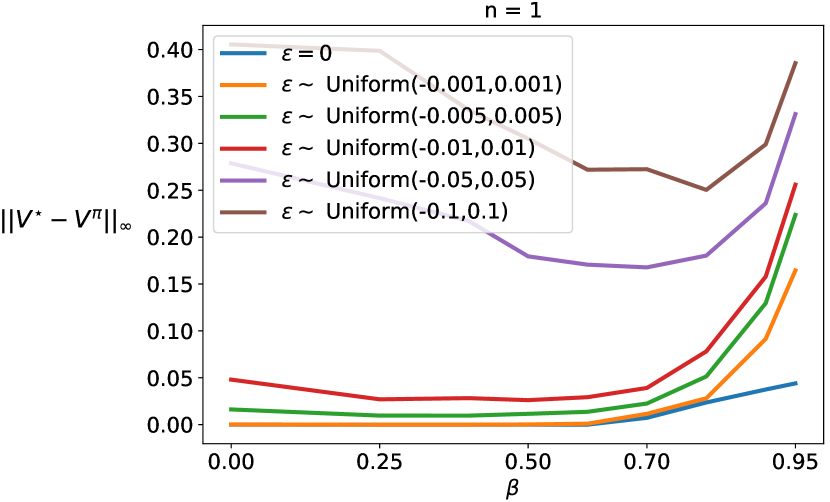
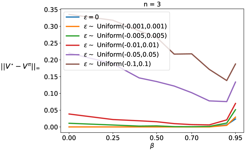
Figure 1: Performance of approximate PMPI has a U-shaped dependence on the parameter $\beta=\frac{1}{1+c}$. Results are averaged over 30 random seeds with $n=1$ (left) and $n=3$ (right).

From Figure 1, it is clear that the final performance exhibits a U-shape with respect to the parameter $\beta$. It is also noticable that the best-performing $\beta$ is shifting to the right side (larger values) as we increase the magnitude of noise. This trend makes sense, and is consistent with what is predicted by Theorem 2: As the noise level rises, we have more incentive to use larger (but not too large) $\beta$ values to hedge against it.

5.2 Atari Experiments

In this section, we evaluate the proximal (or Pro) agents relative to their original DQN-style counterparts on the Atari benchmark (Bellemare et al., 2013), and show that endowing the agent with the proximal term can lead into significant improvements in the interim as well as in the final performance. We next investigate the utility of our proposed proximal term through further experiments. Please see the Appendix for a complete description of our experimental pipeline.

5.2.1 Setup

We used 55 Atari games (Bellemare et al., 2013) to conduct our experimental evaluations. Following Machado et al. (2018) and Castro et al. (2018), we used sticky actions to inject stochasticity into the otherwise deterministic Atari emulator.

Our training and evaluation protocols and the hyper-parameter settings follow those of the Dopamine baseline (Castro et al., 2018). To report performance, we measured the undiscounted sum of rewards obtained by the learned policy during evaluation. We further report the learning curve for all experiments averaged across 5 random seeds. We reiterate that we used the exact same hyper-parameters for all agents to ensure a sound comparison.

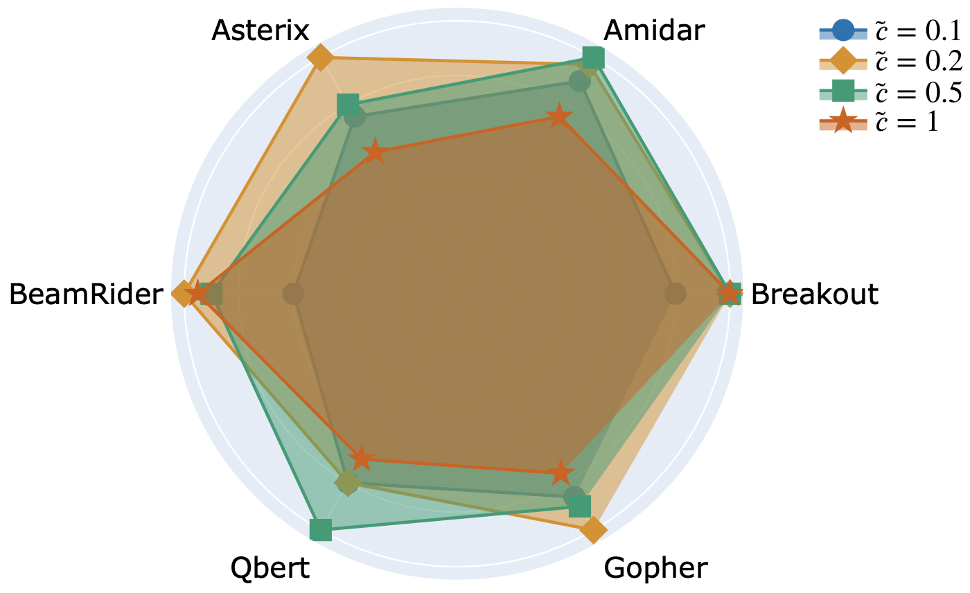
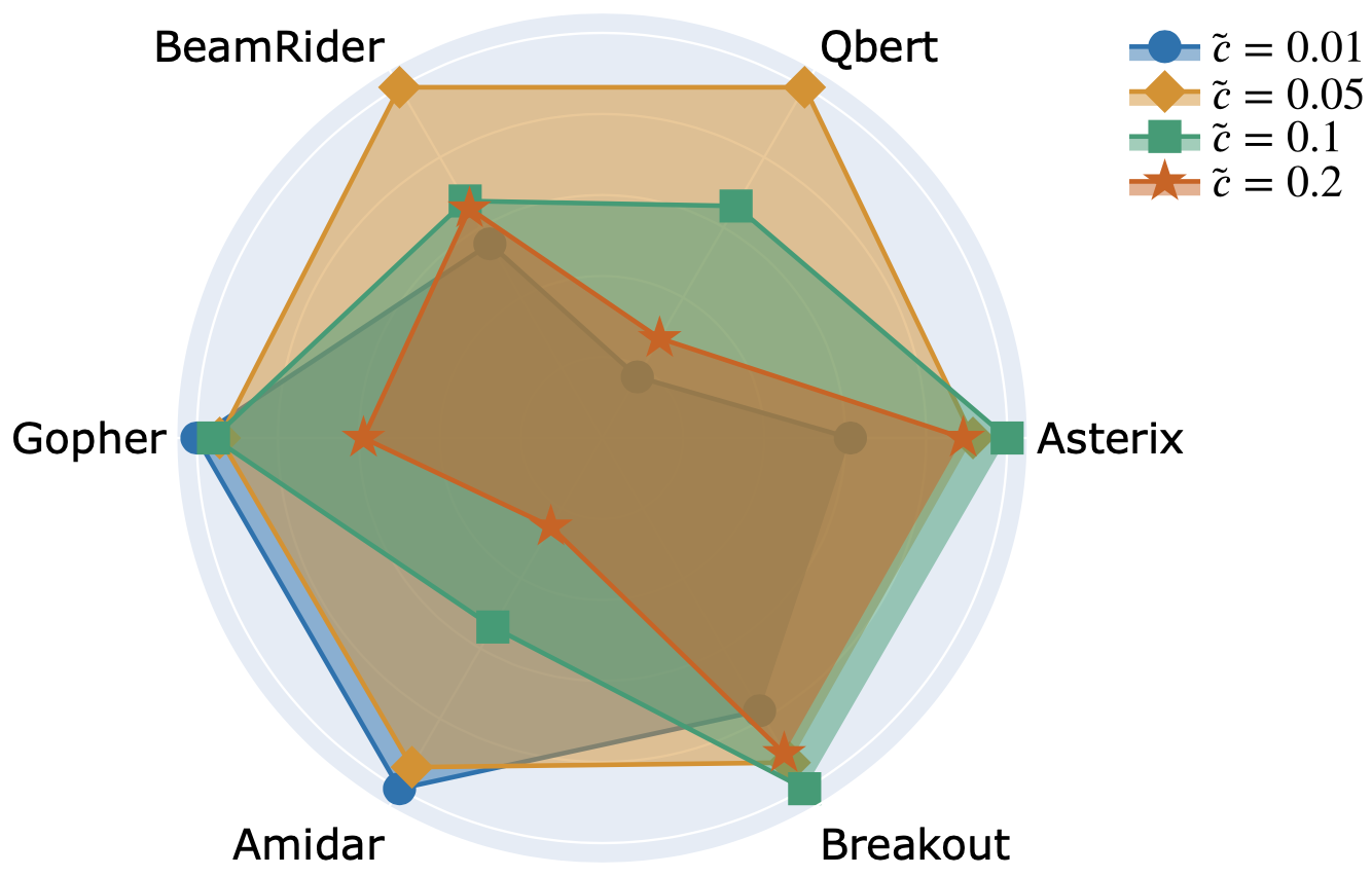
Figure 2: A minimal hyper-parameter tuning for $\tilde{c}$ in DQN Pro (left) and Rainbow Pro (right).

Our Pro agents have a single additional hyper-parameter $\tilde{c}$. We did a minimal random search on 6 games to tune $\tilde{c}$. Figure 2 visualizes the performance of Pro agents as a function of $\tilde{c}$. In light of this result, we set $\tilde{c}=0.2$ for DQN Pro and $\tilde{c}=0.05$ for Rainbow Pro. We used these values of $\tilde{c}$ for all 55 games, and note that we performed no further hyper-parameter tuning at all.

5.2.2 Results

The first question is whether endowing the DQN agent with the proximal term can yield significant improvements over the original DQN.

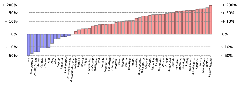
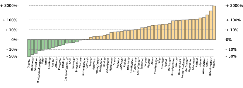
Figure 3: Final gain for DQN Pro over DQN (top), and Rainbow Pro over Rainbow (bottom), averaged over 5 seeds. DQN Pro and Rainbow Pro significantly outperform their original counterparts.

Figure 3 (top) shows a comparison between DQN and DQN Pro in terms of the final performance. In particular, following standard practice (Wang et al., 2016; Dabney et al., 2018; van Seijen et al., 2019), for each game we compute:

$$\frac{\textrm{Score}_{\textrm{DQN Pro}}-\textrm{Score}_{\textrm{DQN}}}{\max(\textrm{Score}_{\textrm{DQN}},\textrm{Score}_{\textrm{Human}})-\textrm{Score}_{\textrm{Random}}}\ .$$

Bars shown in red indicate the games in which we observed better final performance for DQN Pro relative to DQN, and bars in blue indicate the opposite. The height of a bar denotes the magnitude of this improvement for the corresponding benchmark; notice that the y-axis is scaled logarithmically. We took human and random scores from previous work (Nair et al., 2015; Dabney et al., 2018). It is clear that DQN Pro dramatically improves upon DQN. We defer to the Appendix for full learning curves on all games tested.

Can we fruitfully combine the proximal term with some of the existing algorithmic improvements in DQN? To answer this question, we build on the Rainbow algorithm of Hessel et al. (2018) who successfully combined numerous important algorithmic ideas in the value-based RL literature. We present this result in Figure 3 (bottom). Observe that the overall trend is for Rainbow Pro to yield large performance improvements over Rainbow.

Additionally, we measured the performance of our agents relative to human players. To this end, and again following previous work (Wang et al., 2016; Dabney et al., 2018; van Seijen et al., 2019), for each agent we compute the human-normalized score:

$$\frac{\textrm{Score}_{\textrm{Agent}}-\textrm{Score}_{\textrm{Random}}}{\textrm{Score}_{\textrm{Human}}-\textrm{Score}_{\textrm{Random}}}.$$

In Figure 4 (left), we show the median of this score for all agents, which Wang et al. (2016) and Hessel et al. (2018) argued is a sensible quantity to track. We also show per-game learning curves with standard error in the Appendix.

We make two key observations from this figure. First, the very basic DQN Pro agent is capable of achieving human-level performance (1.0 on the y-axis) after 120 million frames. Second, the Rainbow Pro agent achieves 220 percent human-normalized score after only 120 million frames.

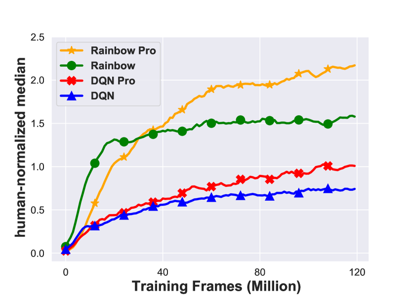
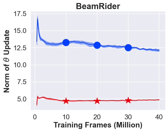
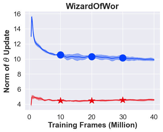
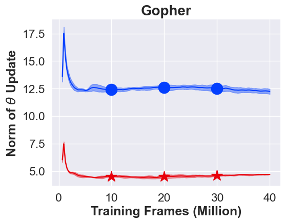
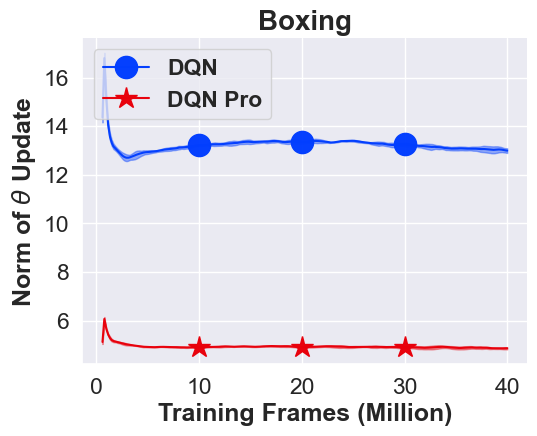
Figure 4: (left): Human-normalized median performance for DQN, Rainbow, DQN Pro, and Rainbow Pro on 55 Atari games. Results are averaged over 5 independent seeds. Our agents, Rainbow Pro (yellow) and DQN Pro (red) outperform their original counterparts Rainbow (green) and DQN (blue). (right): Using the proximal term reduces the magnitude of target network updates.

5.2.3 Additional Experiments

Our purpose in endowing the agent with the proximal term was to keep the online network in the vicinity of the target network, so it would be natural to ask if this desirable property can manifest itself in practice when using the proximal term. In Figure 4, we answer this question affirmatively by plotting the magnitude of the update to the target network during synchronization. Notice that we periodically synchronize online and target networks, so the proximity of the online and target network should manifest itself in a low distance between two consecutive target networks. Indeed, the results demonstrate the success of the proximal term in terms of obtaining the desired proximity of online and target networks.

While using the proximal term leads to significant improvements, one may still wonder if the advantage of DQN Pro over DQN is merely stemming from a poorly-chosen period hyper-parameter in the original DQN, as opposed to a truly more stable optimization in DQN Pro. To refute this hypothesis, we ran DQN with various settings of the period hyper-parameter $\{2000,4000,8000,12000\}$. This set included the default value of the hyper-parameter (8000) from the original paper (Mnih et al., 2015), but also covered a wider set of settings.

Additionally, we tried an alternative update strategy for the target network, referred to as Polyak averaging, which was popularized in the context of continuous-action RL (Lillicrap et al., 2015): $\theta\leftarrow\tau w+(1-\tau)\theta$. For this update strategy, too, we tried different settings of the $\tau$ hyper-parameter, namely $\{0.05,0.005,0.0005\}$, which includes the value $0.005$ used in numerous papers (Lillicrap et al., 2015; Fujimoto et al., 2018; Asadi et al., 2021).

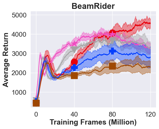
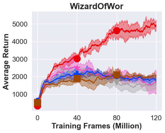
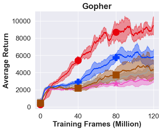
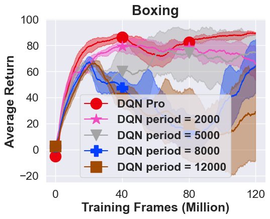
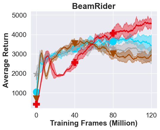
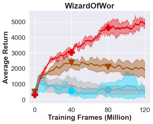
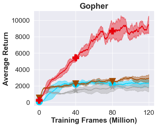
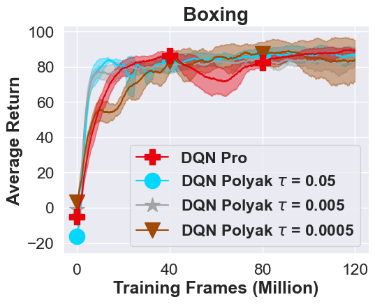
Figure 5: A comparison between DQN Pro and DQN with periodic (left) and Polyak (right) updates.

Figure 5 presents a comparison between DQN Pro and DQN with periodic and Polyak target updates for various hyper-parameter settings of period and $\tau$. It is clear that DQN Pro is consistently outperforming the two alternatives regardless of the specific values of period and $\tau$, thus clearly demonstrating that the improvement is stemming from a more stable optimization procedure leading to a better interplay between the two networks.

Finally, an alternative approach to ensuring lower distance between the online and the target network is to anneal the step size based on the number of updates performed on the online network since the last online-target synchronization. In this case we performed this experiment in 4 games where we knew proximal updates provide improvements based on our DQN Pro versus DQN resulst in Figure 3. In this case we linearly decreased the step size from the original DQN learning rate $\alpha$ to $\alpha^{\prime}\ll\alpha$ where we tuned $\alpha^{\prime}$ using random search. Annealing indeed improves DQN, but DQN Pro outperforms the improved version of DQN. Our intuition is that Pro agents only perform small updates when the target network is far from the online network, but naively decaying the learning rate can harm progress when the two networks are in vicinity of each other.

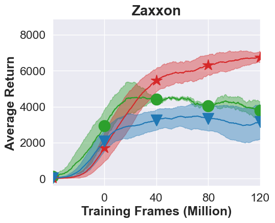
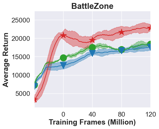
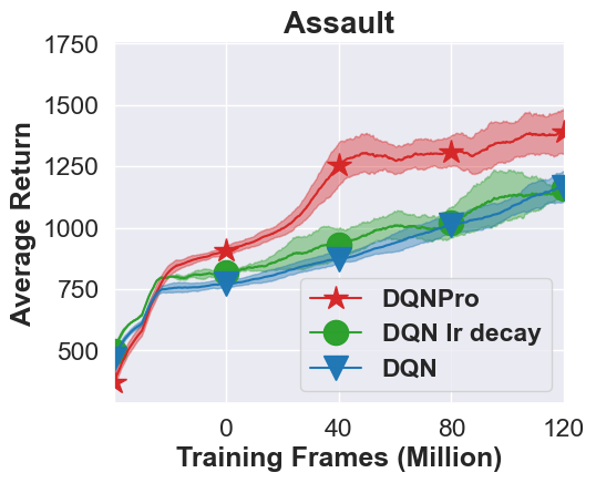
Figure 6: Learning-rate decay does not bridge the gap between DQN and DQN Pro.

6 Discussion

In our experience using proximal updates in the parameter space were far superior than proximal updates in the value space. We believe this is because the parameter-space definition can enforce the proximity globally, while in the value space one can only hope to obtain proximity locally and on a batch of samples. One may hope to use natural gradients to enforce value-space proximity in a more principled way, but doing so usually requires significantly more computational resources Knight & Lerner (2018). This is in contrast to our proximal updates which add negligible computational cost in the simple form of taking a dimension-wise weighted average of two weight vectors.

In addition, for a smooth (Lipschitz) $Q$ function, performing parameter-space regularization guarantees function-space regularization. Concretely: $\forall s,\forall a\ |Q(s,a;\theta)-Q(s,a;\theta^{\prime})|\leq L||\theta-\theta^{\prime}||\ ,$ where $L$ is the Lipschitz constant of $Q$. Moreover, deep networks are Lipschitz (Neyshabur et al., 2015; Asadi et al., 2018), because they are constructed using compositions of Lipschitz functions (such as ReLU, convolutions, etc) and that composition of Lipschitz functions is Lipschitz. So performing value-space updates may be an overkill. Lipschitz property of deep networks has successfully been leveraged in other contexts, such as in generative adversarial training Arjovsky et al. (2017).

A key selling point of our result is simplicity, because simple results are easy to understand, implement, and reproduce. We obtained significant performance improvements by adding just a few lines of codes to the publicly available implementations of DQN and Rainbow Castro et al. (2018).

7 Related Work

The introduction of proximal operators could be traced back to the seminal work of Moreau (1962, 1965), Martinet (1970) and Rockafellar (1976), and the use of the proximal operators has since expanded into many areas of science such as signal processing (Combettes & Pesquet, 2009), statistics and machine learning (Beck & Teboulle, 2009; Polson et al., 2015; Reddi et al., 2015), and convex optimization (Parikh & Boyd, 2014; Bertsekas, 2011b, a).

In the context of RL, Mahadevan et al. (2014) introduced a proximal theory for deriving convergent off-policy algorithms with linear function approximation. One intriguing characteristic of their work is that they perform updates in primal-dual space, a property that was leveraged in sample complexity analysis (Liu et al., 2020) for the proximal counterparts of the gradient temporal-difference algorithm (Sutton et al., 2008). Proximal operators also have appeared in the deep RL literature. For instance, Fakoor et al. (2020b) used proximal operators for meta learning, and Maggipinto et al. (2020) improved TD3 (Fujimoto et al., 2018) by employing a stochastic proximal-point interpretation.

The effect of the proximal term in our work is reminiscent of the use of trust regions in policy-gradient algorithms (Schulman et al., 2015, 2017; Wang et al., 2019; Fakoor et al., 2020a; Tomar et al., 2021). However, three factors differentiate our work: we define the proximal term using the value function, not the policy, we enforce the proximal term in the parameter space, as opposed to the function space, and we use the target network as the previous iterate in our proximal definition.

8 Conclusion and Future work

We showed a clear advantage for using proximal terms to perform slower but more effective updates in approximate planning and reinforcement learning. Our results demonstrated that proximal updates lead to more robustness with respect to noise. Several improvements to proximal methods exist, such as the acceleration algorithm (Nesterov, 1983; Li & Lin, 2015), as well as using other proximal terms (Combettes & Pesquet, 2009), which we leave for future work.

9 Acknowledgment

We thank Lihong Li, Pratik Chaudhari, and Shoham Sabach for their valuable insights in different stages of this work.

10 Appendix

10.1 Pseudo-code for DQN Pro

Below, we present the pseudo-code for DQN Pro. Notice that the difference between DQN and DQN Pro is minimal (highlighted in gray).

Algorithm 1 DQN with Proximal Iteration (DQN Pro)

1:Initialize $\theta$, N, period, replay buffer $\mathcal{D},\alpha,$ and ${\boldsymbol{\tilde{c}}}$

2:$s\leftarrow$ env.reset(), $w\leftarrow\theta$, $\textrm{numUpdates}\leftarrow 0$

3:repeat

4:     $a\sim\epsilon$-greedy($Q(s,\cdot;w$))

5:     $s^{\prime},r\leftarrow\$env.step($s,a$)

6:     add $\langle s,a,r,s^{\prime}\rangle$ to $\mathcal{D}$

7:     if $s^{\prime}$ is terminal then

8:         $s\leftarrow$ env.reset()

9:     end if

10:     for $n$ in {1, …, N} do

11:         sample $\mathcal{B}=\{\langle s,a,r,s^{\prime}\rangle\}$, compute $\nabla_{w}h(w)$

12:         $w\!\leftarrow\!{\big{(}1-(\alpha/\tilde{c})\big{)}w+(\alpha/\tilde{c})\theta}-\alpha\nabla_{w}h(w)$

13:         $\textrm{numUpdates}\leftarrow\textrm{numUpdates}+1$

14:         if $\textrm{numUpdates}\ \%\ \textit{period}=0$ then

15:              $\theta\leftarrow w$

16:         end if

17:     end for

18:until convergence

10.2 Implementation Details

Table 1 and 2 show hyper-parameters, computing infrastructure, and libraries used for the experiments in this paper for all games tested. Our training and evaluation protocols and the hyper-parameter settings closely follow those of the Dopamine baseline. To report performance results, we measured the undiscounted sum of rewards obtained by the learned policy during evaluation.

DQN hyper-parameters (shared)
Replay buffer size	$200000$
Target update period	$8000$
Max steps per episode	$27000$
Evaluation frequency	$10000$
Batch size	$64$
Update period	$4$
Number of frame skip	$4$
Number of episodes to evaluate	$2$
Update horizon	$1$
$\epsilon$-greedy (training time)	$0.01$
$\epsilon$-greedy (evaluation time)	$0.001$
$\epsilon$-greedy decay period	$250000$
Burn-in period / Min replay size	$20000$
Learning rate	$10^{-4}$
Discount factor ($\gamma$)	$0.99$
Total number of iterations	$3\times 10^{7}$
Sticky actions	True
Optimizer	Adam Kingma & Ba (2015)
Network architecture	Nature DQN network Mnih et al. (2015)
Random seeds	$\{0,1,2,3,4\}$
Rainbow hyper-parameters (shared)
Batch size	64
Other	Config file rainbow_aaai.gin from Dopamine
DQN Pro and Rainbow Pro hyper-parameter
$\tilde{c}\ \textrm{(DQN Pro)}$	$0.2$
$\tilde{c}\ \textrm{(Rainbow Pro)}$	$0.05$

Table 1: Hyper-parameters used for all methods for all 55 games of Atari-2600 benchmarks

. All results reported in our paper are averages over repeated runs initialized with each of the random seeds listed above and run for the listed number of episodes.

Computing Infrastructure
Machine Type	AWS EC2 - p2.16xlarge
GPU Family	Tesla K80
CPU Family	Intel Xeon 2.30GHz
CUDA Version	$11.0$
NVIDIA-Driver	$450.80.02$
Library Version
Python	$3.8.5$
Numpy	$1.20.1$
Gym	$0.18.0$
Pytorch	$1.8.0$

Table 2: Computing infrastructure and software libraries used in all experiments in this paper.

10.3 Proofs

See 1 We make two assumptions:

1. $f$ is smooth, or more specifically that its gradient is 1-Lipschitz: $||\nabla f(v_{1})-\nabla f(v_{2})||\leq||v_{1}-v_{2}||\ \forall v_{1},\forall v_{2}$ .

2. the value of the parameter $c$ is large, in particular $c>\frac{2}{1-\gamma}\$.

Proof.

Both terms are convex and differentiable, therefore by setting the gradient to zero, we have:

$$\mathcal{T}^{\star}_{c,f}v=\mathcal{T}^{\star}v+\frac{1}{c}\big{(}\nabla f(v)-\nabla f(\mathcal{T}^{\star}_{c,f}v)\big{)},$$

We can then show:

$$||\mathcal{T}^{\star}_{c,f}v_{1}-\mathcal{T}^{\star}_{c,f}v_{2}|| = ||T^{\star}v_{1}+\frac{1}{c}\big{(}\nabla f(v_{1})-\nabla f(\mathcal{T}^{\star}_{c,f}v_{1})\big{)}-T^{\star}v_{2}-\frac{1}{c}\big{(}\nabla f(v_{2})-\nabla f(\mathcal{T}^{\star}_{c,f}v_{2})\big{)}||$$

$$\leq ||T^{\star}v_{1}-T^{\star}v_{2}||+\frac{1}{c}||\nabla f(v_{1})-\nabla f(v_{2})||+\frac{1}{c}||\nabla f(\mathcal{T}^{\star}_{c,f}v_{1})-\nabla f(\mathcal{T}^{\star}_{c,f}v_{2})||$$

(first assumption)

$$\leq ||T^{\star}v_{1}-T^{\star}v_{2}||+\frac{1}{c}||\nabla f(v_{1})-\nabla f(v_{2})||+\frac{1}{c}||\mathcal{T}^{\star}_{c,f}v_{1}-\mathcal{T}^{\star}_{c,f}v_{2}||$$

This implies:

$$\frac{c-1}{c}||\mathcal{T}^{\star}_{c,f}v_{1}-\mathcal{T}^{\star}_{c,f}v_{2}|| \leq ||T^{\star}v_{1}-T^{\star}v_{2}||+\frac{1}{c}||\nabla f(v_{1})-\nabla f(v_{2})||$$

(first assumption)

$$\leq ||T^{\star}v_{1}-T^{\star}v_{2}||+\frac{1}{c}||v_{1}-v_{2}||$$

$$\leq \frac{\gamma c+1}{c}||v_{1}-v_{2}||$$

Therefore,

$$||\mathcal{T}^{\star}_{c,f}v_{1}-\mathcal{T}^{\star}_{c,f}v_{2}|| \leq \frac{\gamma c+1}{c-1}||v_{1}-v_{2}||\ ,$$

Allowing us to conclude that $\mathcal{T}^{\star}_{c,f}$ is a contraction (second assumption).

Further, to show that $v^{\star}$ is indeed the fixed point of $\mathcal{T}^{\star}_{c,f}$, notice from the original formulation:

$$\mathcal{T}^{\star}_{c,f}v\vcentcolon=\arg\min_{v^{\prime}}||v^{\prime}-\mathcal{T}^{\star}v||^{2}_{2}+\frac{1}{c}D_{f}(v^{\prime},v)\ ,$$

that, at point $v^{*}$ setting $v^{\prime}=v^{\star}$ jointly minimizes the first term, because $v^{\star}=\mathcal{T}^{\star}v^{\star}$ due to fixed-point defintion, and it also minimizes the second term because $D_{f}(v^{\star},v^{\star})=0$ and that Bregman divergence is non-negative. Therefore, $\mathcal{T}^{\star}_{c,f}v^{\star}=v^{\star}$; $v^{\star}$ is the fixed-point of $\mathcal{T}^{\star}_{c,f}v^{\star}$. Since, $\mathcal{T}^{\star}_{c,f}$ is a contraction, this fixed point is unique. ∎

See 2 We make two assumptions:

1. we assume $\epsilon$ error in policy evaluation step, as already stated in equation (4).

2. we assume $\epsilon^{\prime}$ error in policy greedification step $\pi_{k}\leftarrow\mathcal{G}_{\epsilon^{\prime}_{k}}v_{k-1}\forall k$. This means $\forall\pi\ \mathcal{T}^{\pi}v_{k}-\mathcal{T}^{\pi_{k+1}}v_{k}\leq\epsilon^{\prime}_{k+1}$. Note that this assumption is orthogonal to the thesis of our paper, but we kept it for generality.

Proof.

Step 0: bound the Bellman residual: $b_{k}\vcentcolon=v_{k}-\mathcal{T}^{\pi_{k+1}}v_{k}\ .$

$$b_{k} = v_{k}-\mathcal{T}^{\pi_{k+1}}v_{k}$$

$$= v_{k}-\mathcal{T}^{\pi_{k}}v_{k}+\mathcal{T}^{\pi_{k}}v_{k}-\mathcal{T}^{\pi_{k+1}}v_{k}$$

(from our assumption $$\quad\forall\pi\ \mathcal{T}^{\pi}v_{k}-\mathcal{T}^{\pi_{k+1}}v_{k}\leq\epsilon^{\prime}_{k+1}$$)

$$\leq v_{k}-\mathcal{T}^{\pi_{k}}v_{k}+\epsilon^{\prime}_{k+1}$$

$$= v_{k}-(1-\beta)\epsilon_{k}-\mathcal{T}^{\pi_{k}}v_{k}+(1-\beta)\gamma P^{\pi_{k}}\epsilon_{k}+(1-\beta)\epsilon_{k}-(1-\beta)\gamma P^{\pi_{k}}\epsilon_{k}+\epsilon^{\prime}_{k+1}$$

(from $$\mathcal{T}^{\pi_{k}}v_{k}+(1-\beta)\gamma P^{\pi_{k}}\epsilon_{k}=\mathcal{T}^{\pi_{k}}(v_{k}-(1-\beta)\epsilon_{k}\big{)}$$)

$$= v_{k}-(1-\beta)\epsilon_{k}-\mathcal{T}^{\pi_{k}}(v_{k}-(1-\beta)\epsilon_{k})+(1-\beta)\underbrace{(I-\gamma P_{\pi_{k}})\epsilon_{k}}_{x_{k}}+\epsilon^{\prime}_{k+1}$$

$$= v_{k}-(1-\beta)\epsilon_{k}-\mathcal{T}^{\pi_{k}}(v_{k}-(1-\beta)\epsilon_{k})+(1-\beta)x_{k}+\epsilon^{\prime}_{k+1}$$

(from $$v_{k}-(1-\beta)\epsilon_{k}=(\mathcal{T}^{\pi_{k}}_{\beta})^{n}v_{k-1}$$)

$$= (1-\beta)(\mathcal{T}^{\pi_{k}})^{n}v_{k-1}+\beta v_{k-1}-\mathcal{T}^{\pi_{k}}\big{(}(1-\beta)(\mathcal{T}^{\pi_{k}})^{n}v_{k-1}+\beta v_{k-1}\big{)}+(1-\beta)x_{k}+\epsilon^{\prime}_{k+1}$$

(from linearity of $$\mathcal{T}^{\pi_{k}}$$)

$$= (1-\beta)(\mathcal{T}^{\pi_{k}})^{n}v_{k-1}-\mathcal{T}^{\pi_{k}}\big{(}(1-\beta)(\mathcal{T}^{\pi_{k}})^{n}v_{k-1}\big{)}+\beta\big{(}v_{k-1}-\mathcal{T}^{\pi_{k}}v_{k-1}\big{)}+(1-\beta)x_{k}+\epsilon^{\prime}_{k+1}$$

$$= (1-\beta)\Big{(}(\mathcal{T}^{\pi_{k}})^{n}v_{k-1}-\mathcal{T}^{\pi_{k}}\big{(}(T^{\pi_{k}})^{n}v_{k-1}\big{)}\Big{)}+\beta\big{(}v_{k-1}-\mathcal{T}^{\pi_{k}}v_{k-1}\big{)}+(1-\beta)x_{k}+\epsilon^{\prime}_{k+1}$$

$$= (1-\beta)\Big{(}(\mathcal{T}^{\pi_{k}})^{n}v_{k-1}-(\mathcal{T}^{\pi_{k}})^{n}\big{(}\mathcal{T}^{\pi_{k}}v_{k-1}\big{)}\Big{)}+\beta\big{(}v_{k-1}-\mathcal{T}^{\pi_{k}}v_{k-1}\big{)}+(1-\beta)x_{k}+\epsilon^{\prime}_{k+1}$$

$$= (1-\beta)(\gamma P^{\pi_{k}})^{n}\big{(}\underbrace{v_{k-1}-\mathcal{T}^{\pi_{k}}(v_{k-1}}_{=b_{k-1}})\big{)}+\beta\big{(}\underbrace{v_{k-1}-\mathcal{T}^{\pi_{k}}v_{k-1}}_{=b_{k-1}}\big{)}+(1-\beta)x_{k}+\epsilon^{\prime}_{k+1}\ ,$$

allowing us to conclude:

$$b_{k}=\big{(}(1-\beta)(\gamma P^{\pi_{k}})^{n}+\beta I\big{)}b_{k-1}+(1-\beta)x_{k}+\epsilon^{\prime}_{k+1}\ .$$

Step 1: bound the distance to the optimal value: $d_{k+1}\vcentcolon=v^{*}-(\mathcal{T}^{\pi_{k+1}}_{\beta})^{n}v_{k}\$.

$$d_{k+1} = v^{*}-(\mathcal{T}^{\pi_{k+1}}_{\beta})^{n}v_{k}$$

$$= \mathcal{T}^{\pi^{*}}v^{*}-\mathcal{T}^{\pi^{*}}v_{k}+\underbrace{\mathcal{T}^{\pi^{*}}v_{k}-\mathcal{T}^{\pi_{k+1}}v_{k}}_{\leq\epsilon^{\prime}_{k+1}}+\underbrace{\mathcal{T}^{\pi_{k+1}}v_{k}-(\mathcal{T}^{\pi_{k+1}}_{\beta})^{n}v_{k}}_{=g_{k+1}}$$

$$\leq \gamma P^{\pi^{*}}(v^{*}-v_{k})+\epsilon^{\prime}_{k+1}+g_{k+1}$$

$$= \gamma P^{\pi^{*}}(v^{*}-v_{k})+(1-\beta)\gamma P^{\pi^{*}}\epsilon_{k}-(1-\beta)\gamma P^{\pi^{*}}\epsilon_{k}+\epsilon^{\prime}_{k+1}+g_{k+1}$$

$$= \gamma P^{\pi^{*}}\Big{(}v^{*}-\big{(}v_{k}-(1-\beta)\epsilon_{k}\big{)}\Big{)}-(1-\beta)\underbrace{\gamma P^{\pi^{*}}\epsilon_{k}}_{y_{k}}+\epsilon^{\prime}_{k+1}+g_{k+1}$$

$$= \gamma P^{\pi^{*}}\big{(}\underbrace{v^{*}-(\mathcal{T}^{\pi_{k}}_{\beta})^{n}v_{k-1}}_{=d_{k}}\big{)}-(1-\beta)y_{k}+\epsilon^{\prime}_{k+1}+g_{k+1}$$

$$= \gamma P^{\pi^{*}}d_{k}-(1-\beta)y_{k}+\epsilon^{\prime}_{k+1}+g_{k+1}$$

Additionally we can bound $g_{k+1}$ as follows:

$$g_{k+1} = \mathcal{T}^{\pi_{k+1}}v_{k}-(\mathcal{T}^{\pi_{k+1}}_{\beta})^{n}v_{k}$$

$$= (1-\beta)\big{(}\mathcal{T}^{\pi_{k+1}}v_{k}-(\mathcal{T}^{\pi^{k+1}})^{n}v_{k}\big{)}+\beta(T^{\pi_{k+1}}v_{k}-v_{k})$$

$$= (1-\beta)\sum_{j=1}^{n-1}(\gamma P^{\pi_{k+1}})^{j}b_{k}+\beta(-b_{k})$$

Allowing us to conclude that:

$$d_{k+1}\leq\gamma P^{\pi^{*}}d_{k}-\big{(}(1-\beta)y_{k}+\beta b_{k}\big{)}+(1-\beta)\sum_{j=1}^{n-1}(\gamma P^{\pi_{k+1}})^{j}b_{k}+\epsilon^{\prime}_{k+1}$$

Step 2: bound the distance between the approximate value and the value of the policy: $s_{k}\vcentcolon=(T^{\pi_{k}}_{\beta})^{n}v_{k-1}-v^{\pi_{k}}\$.

$$s_{k} = (T^{\pi_{k}}_{\beta})^{n}v_{k-1}-v^{\pi_{k}}$$

$$= (T^{\pi_{k}}_{\beta})^{n}v_{k-1}-(\mathcal{T}^{\pi_{k}})^{\infty}v_{k-1}$$

$$= (1-\beta)(\mathcal{T}^{\pi_{k}})^{n}v_{k-1}+\beta v_{k-1}-(1-\beta)(\mathcal{T}^{\pi_{k}})^{\infty}v_{k-1}-\beta(\mathcal{T}^{\pi_{k}})^{\infty}v_{k-1}$$

$$= (1-\beta)\big{(}(\mathcal{T}^{\pi_{k}})^{n}v_{k-1}-(\mathcal{T}^{\pi_{k}})^{\infty}v_{k-1}\big{)}+\beta\big{(}v_{k-1}-(\mathcal{T}^{\pi_{k}})^{\infty}v_{k-1}\big{)}$$

$$= (1-\beta)(\gamma P^{\pi_{k}})^{n}\big{(}v_{k-1}-(\mathcal{T}^{\pi_{k}})^{\infty}v_{k-1}\big{)}+\beta\big{(}v_{k-1}-(\mathcal{T}^{\pi_{k}})^{\infty}v_{k-1}\big{)}$$

$$= \big{(}(1-\beta)(\gamma P^{\pi_{k}})^{n}+\beta I\big{)}\big{(}v_{k-1}-(\mathcal{T}^{\pi_{k}})^{\infty}v_{k-1}\big{)}$$

$$= \big{(}(1-\beta)(\gamma P^{\pi_{k}})^{n}+\beta I\big{)}(I-\gamma P^{\pi_{k}})^{-1}\big{(}\underbrace{v_{k-1}-\mathcal{T}^{\pi_{k}}v_{k-1}}_{b_{k-1}}\big{)}\ .$$

Allowing us to conclude that:

$$s_{k}=\big{(}(1-\beta)(\gamma P^{\pi_{k}})^{n}+\beta I\big{)}(I-\gamma P^{\pi_{k}})^{-1}b_{k-1}\ .$$

∎

11 Learning curves

We present full learning curves of DQN, DQN Pro, Rainbow, and Rainbow Pro for the 55 Atari games. All results are averaged over 5 independent seeds.

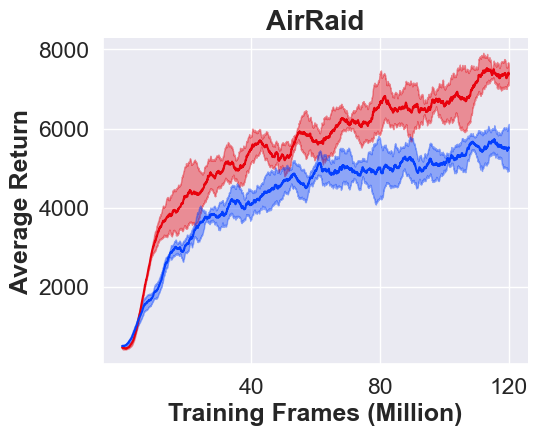
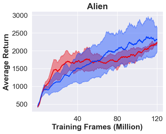
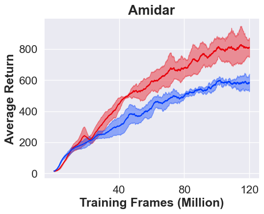
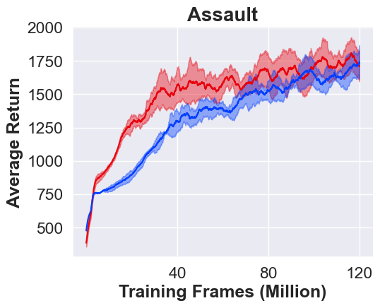
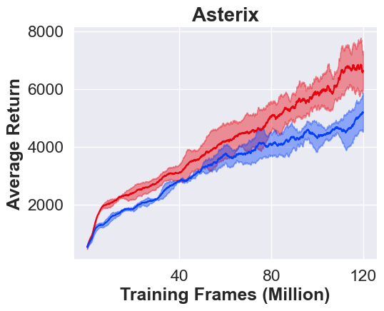
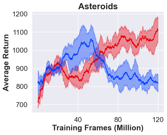
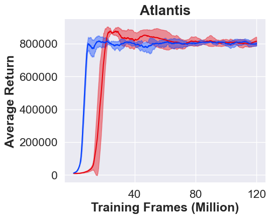
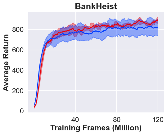
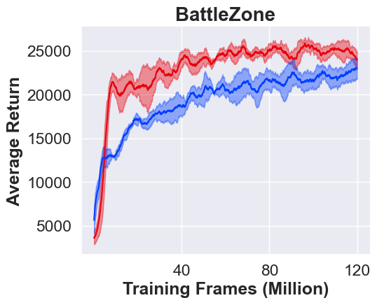
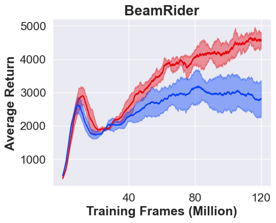
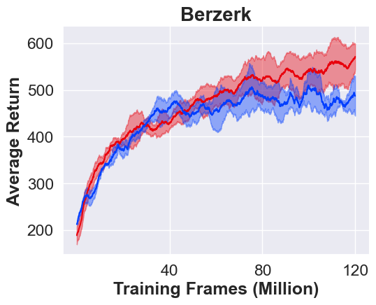
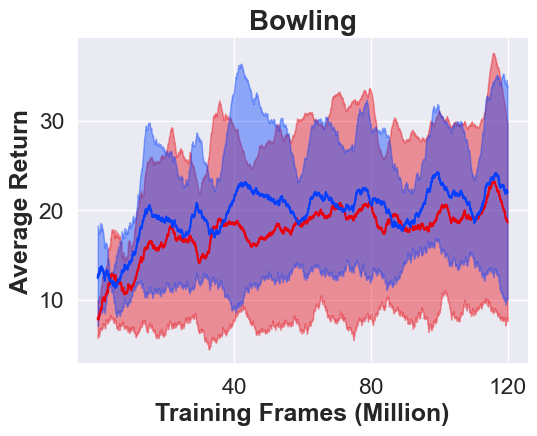
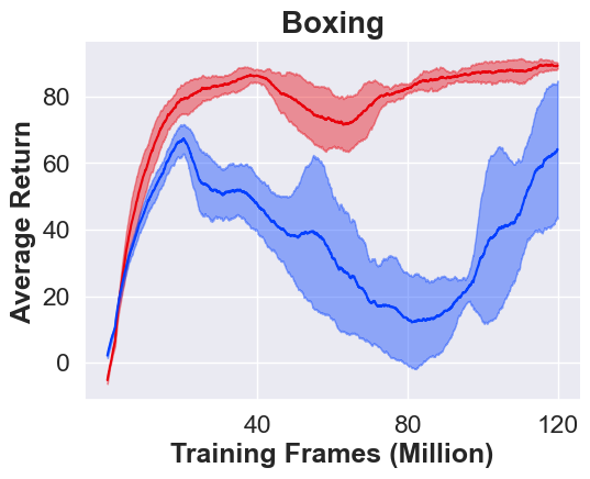
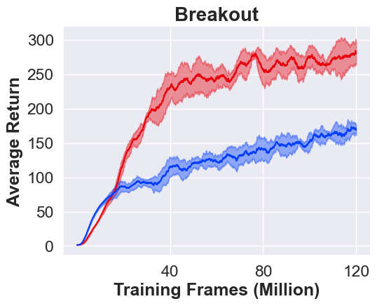
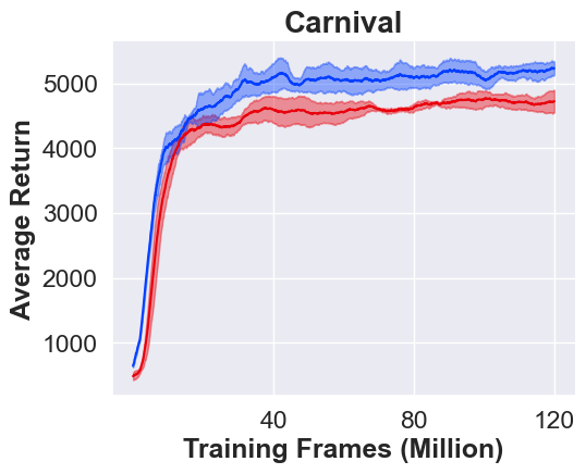
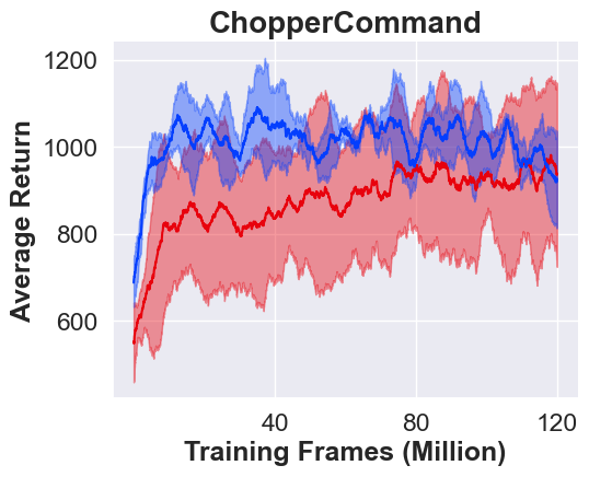
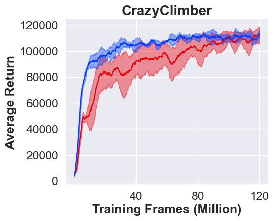
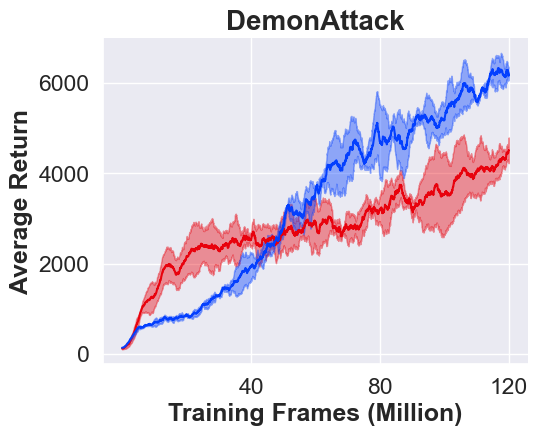
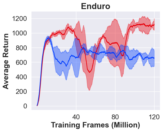
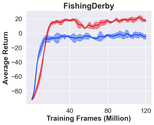
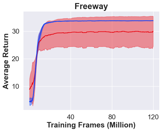
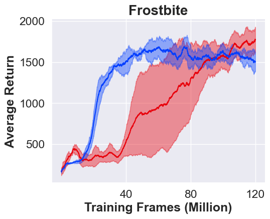
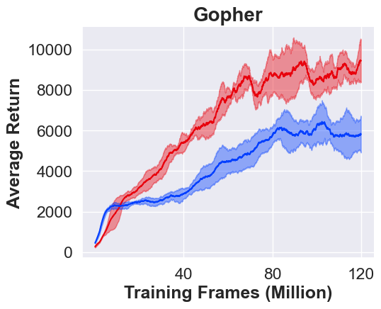
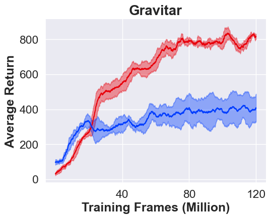
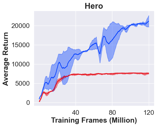
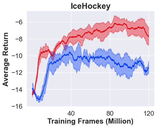
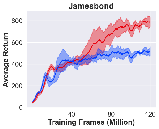
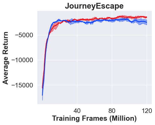
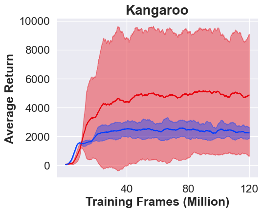
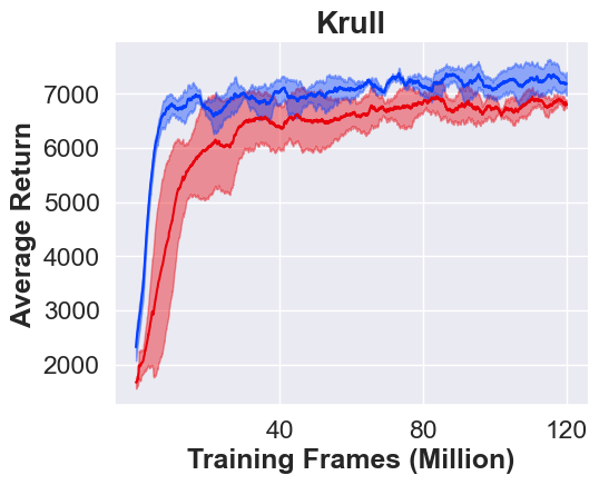
Figure 7: Comparison between DQN Pro (red) and DQN (blue) over 55 Atari games (Part I).

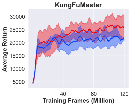
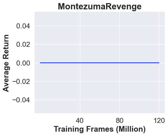
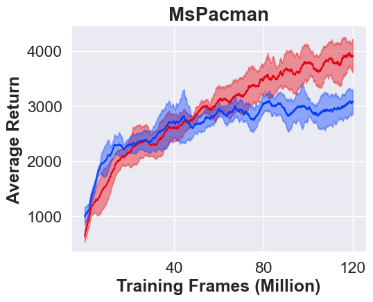
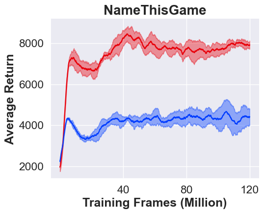
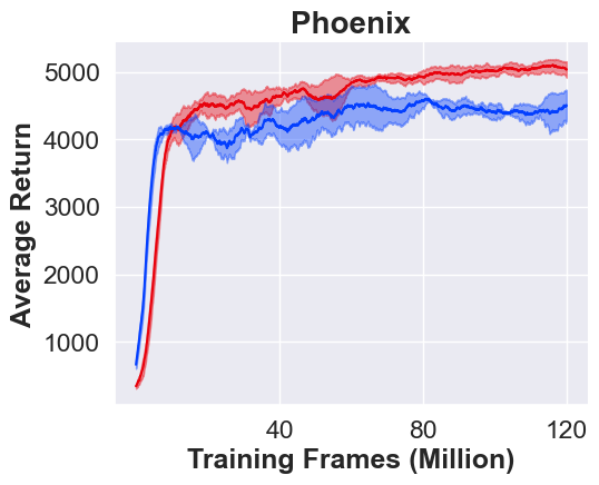
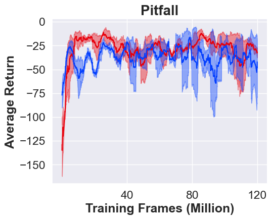
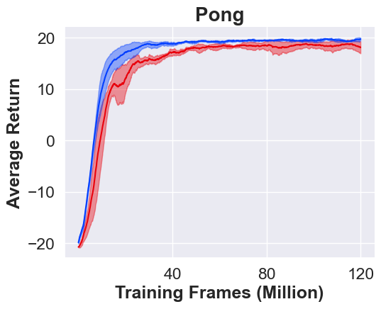
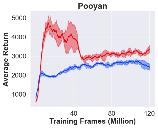
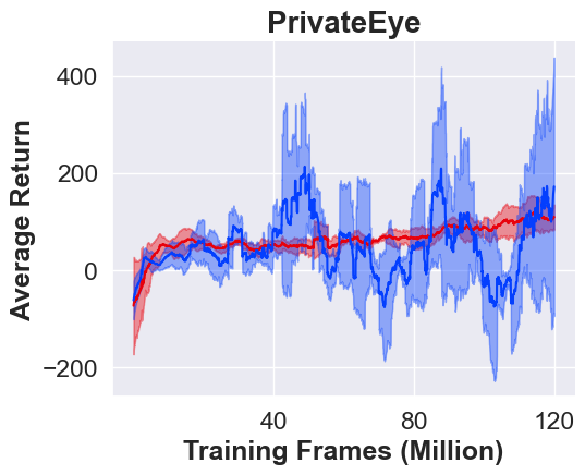
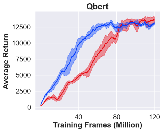
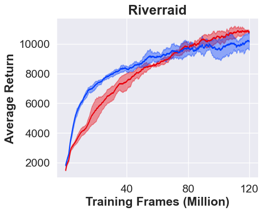
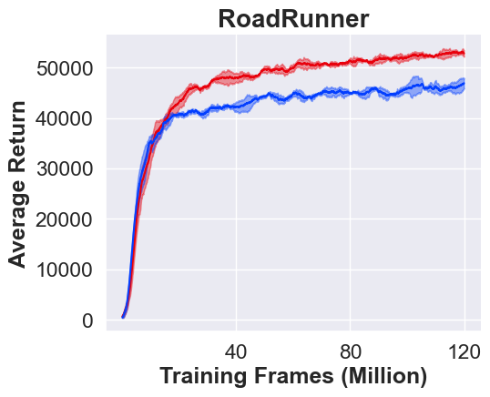
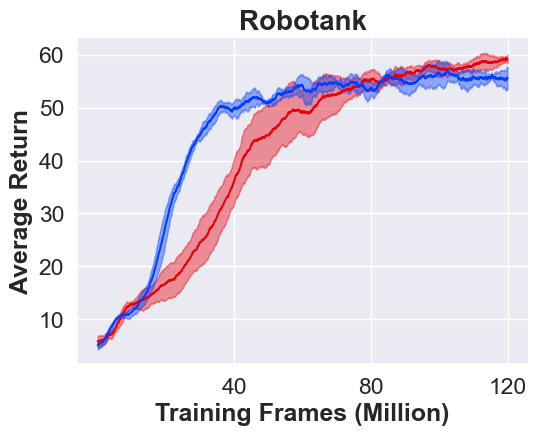
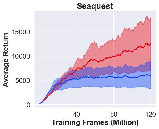
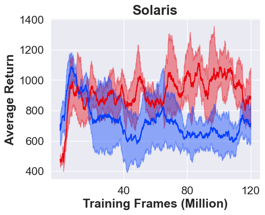
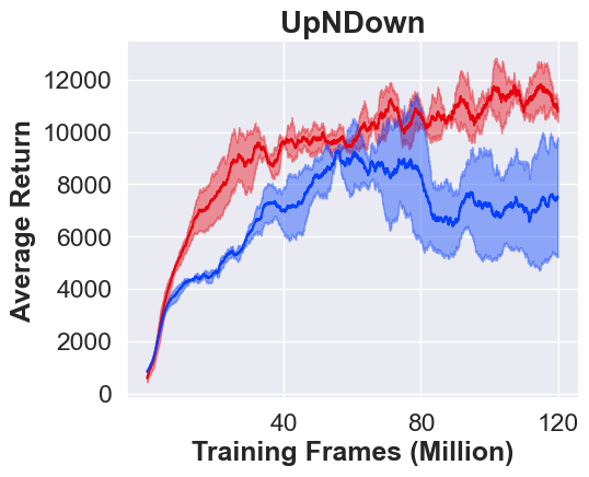
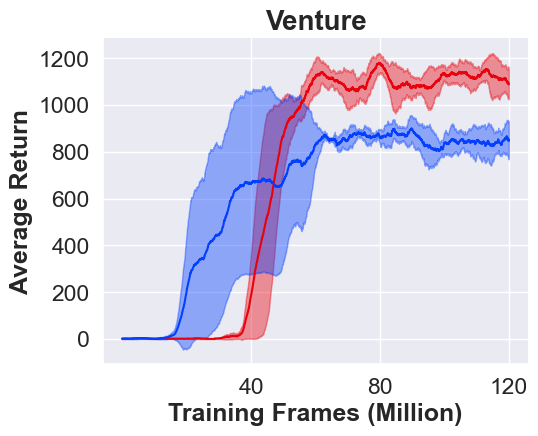
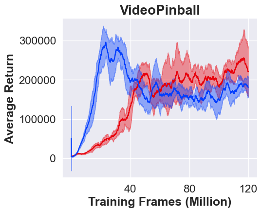
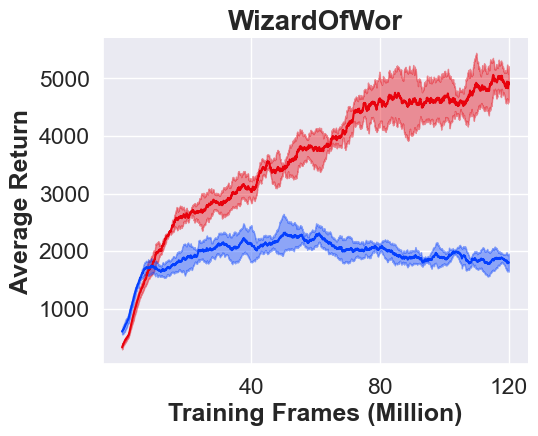
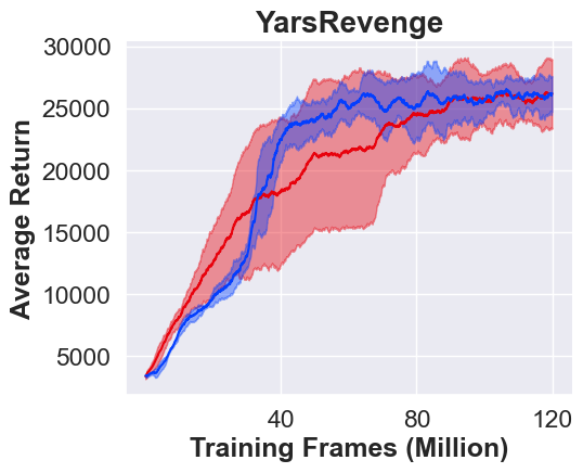
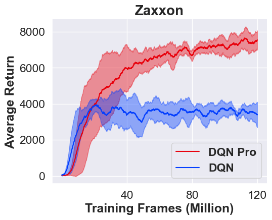
Figure 8: Comparison between DQN Pro (red) and DQN (blue) over 55 Atari games (Part II).

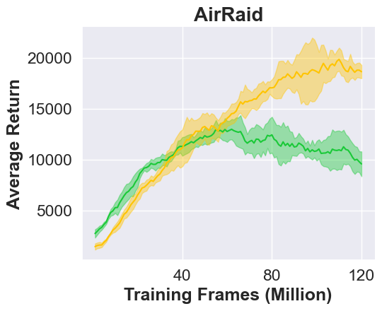
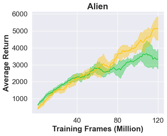
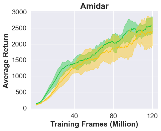
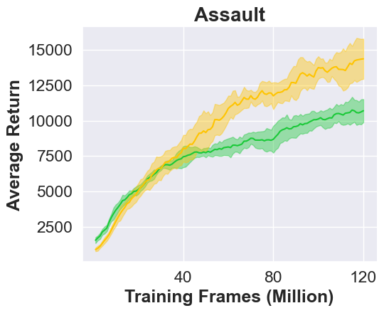
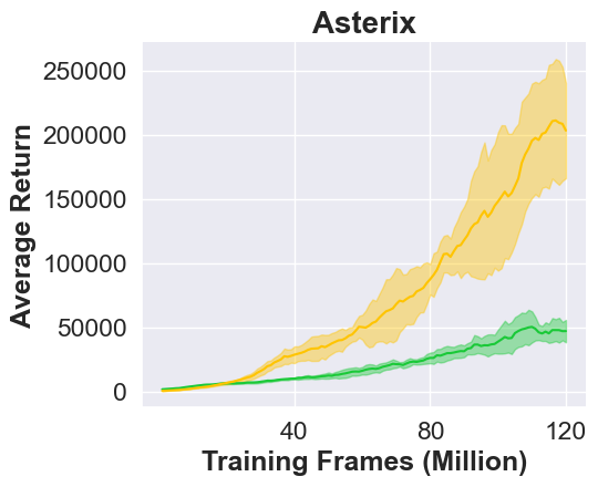
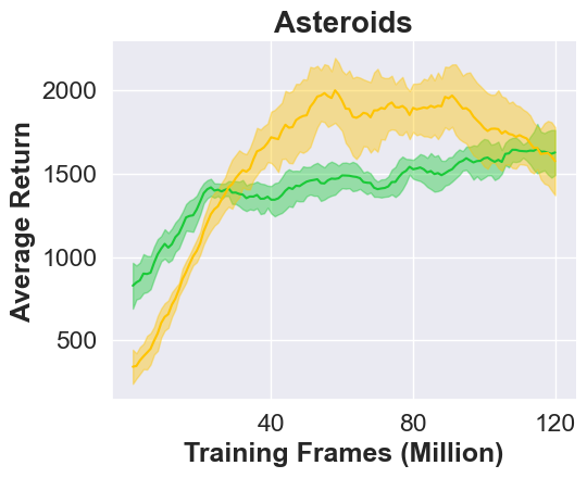
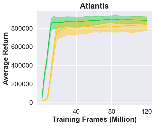
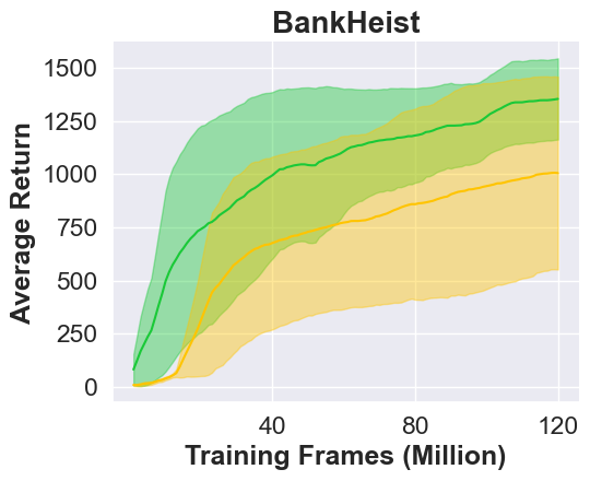
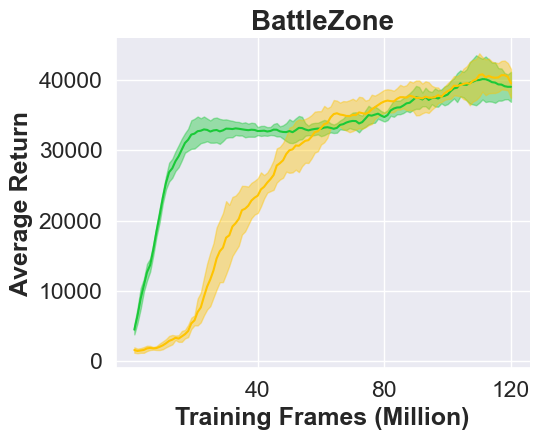
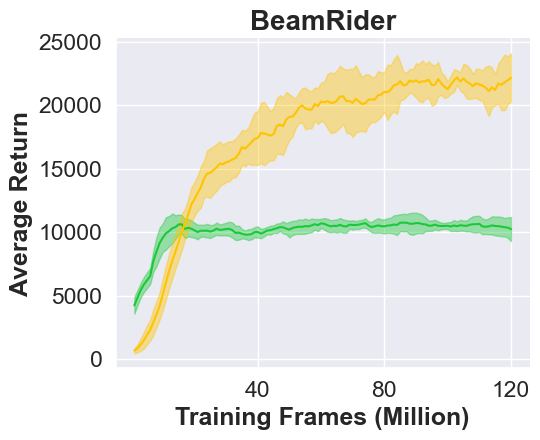
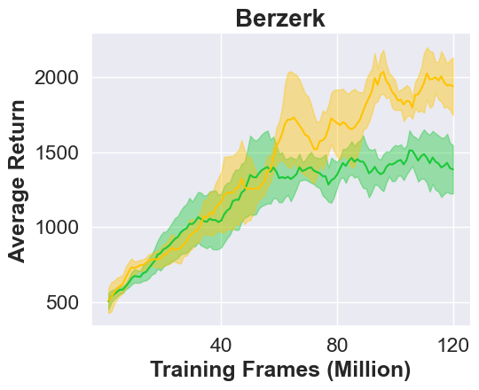
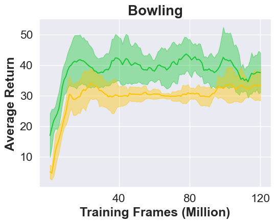
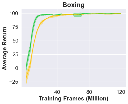
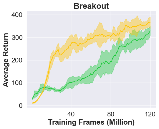
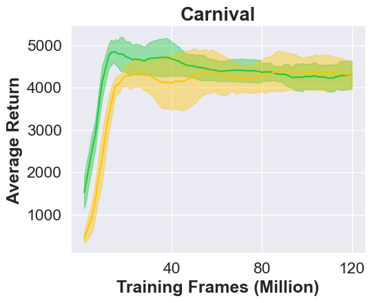
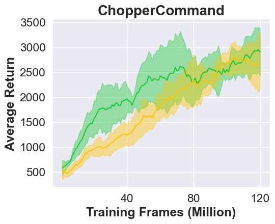
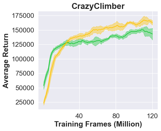
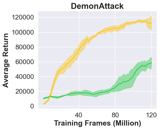
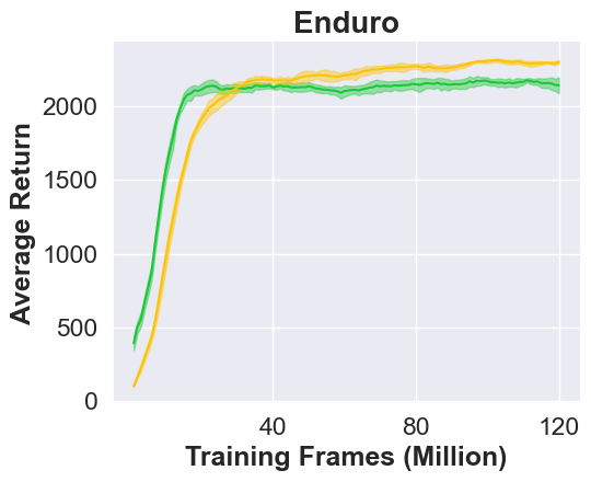
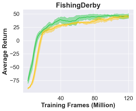
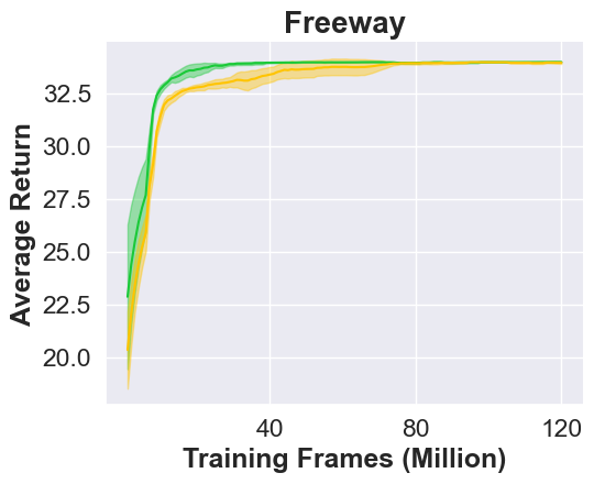
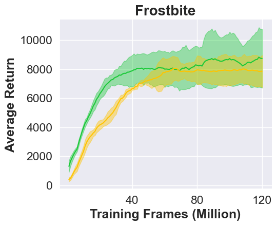
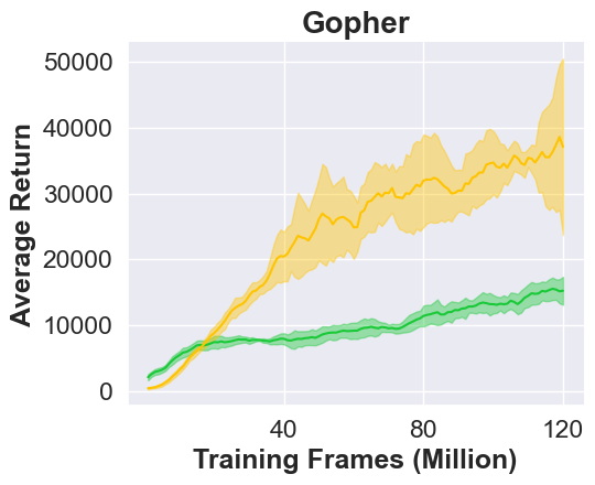
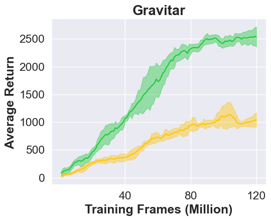
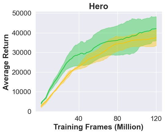
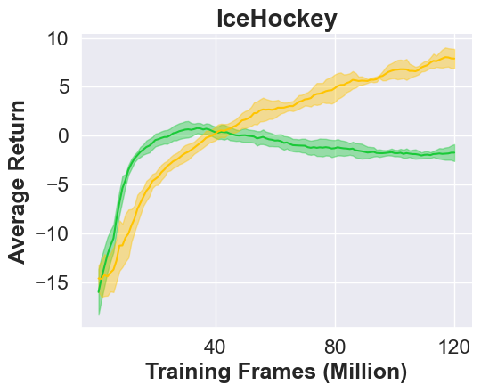
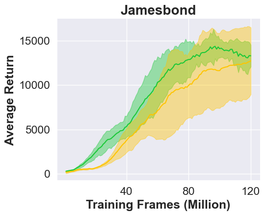
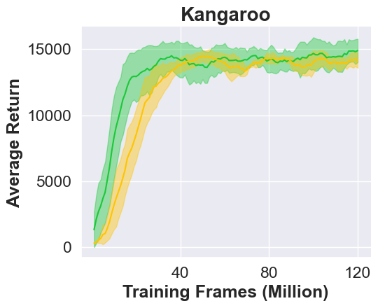
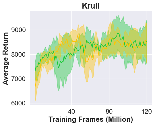
Figure 9: Comparison between Rainbow Pro (yellow) and Rainbow (green) over 55 Atari games (Part I).

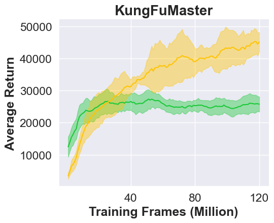
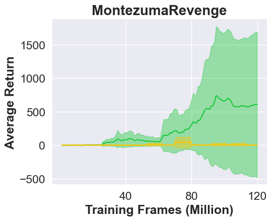
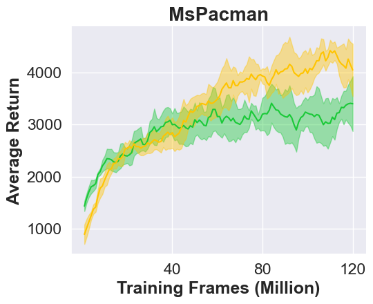
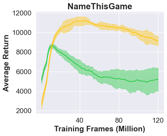
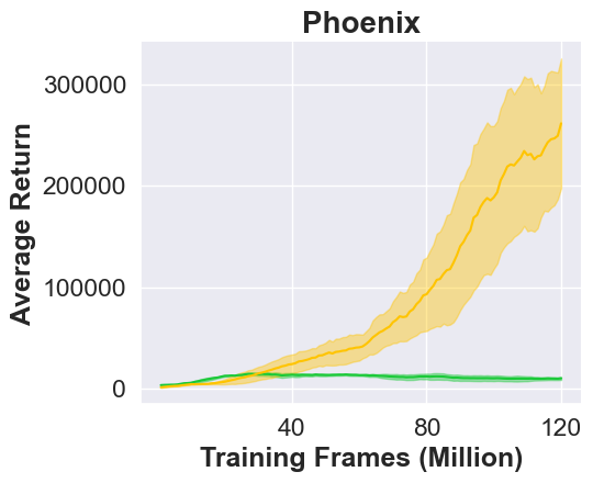
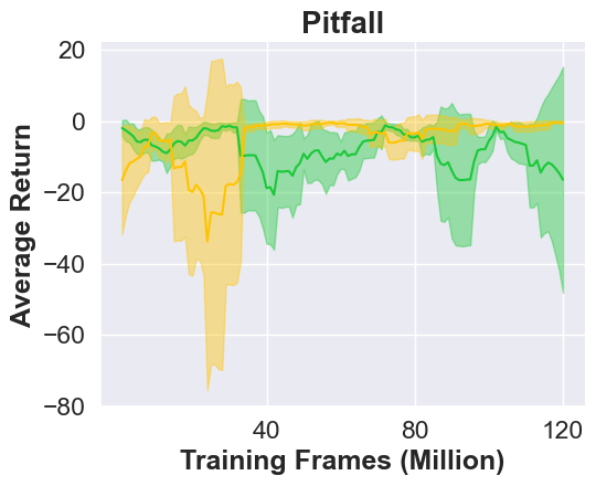
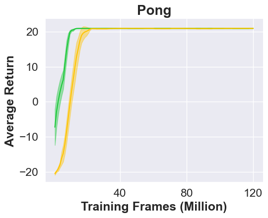
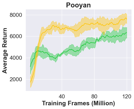
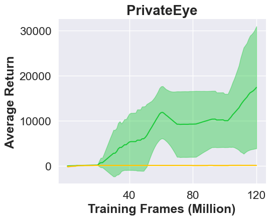
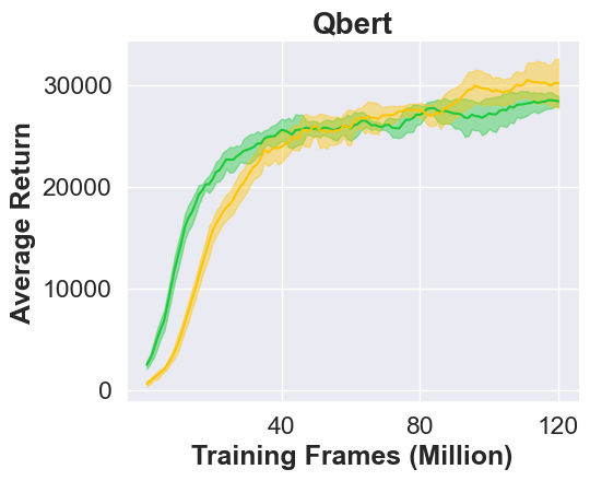
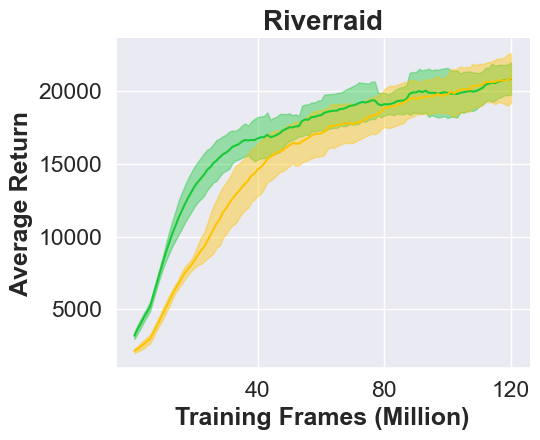
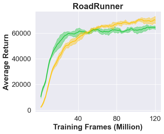
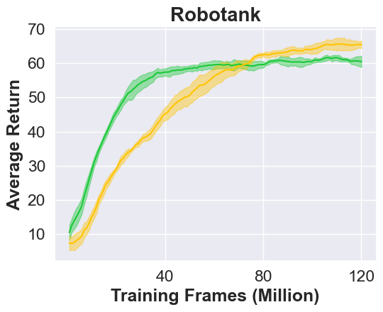
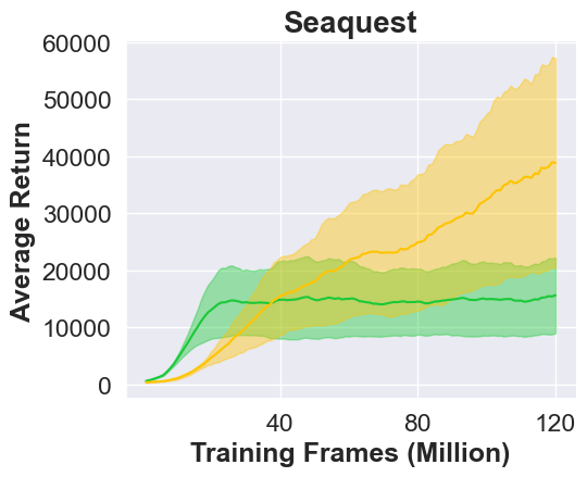
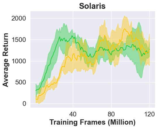
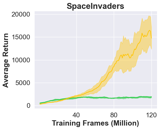
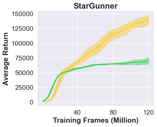
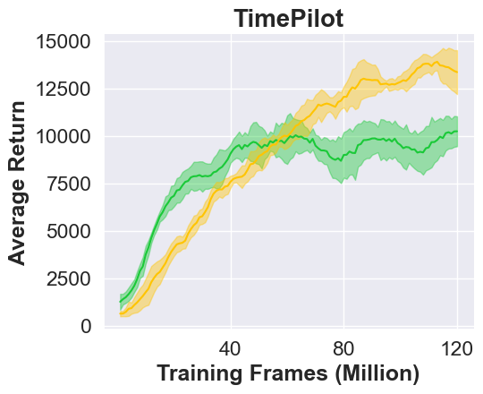
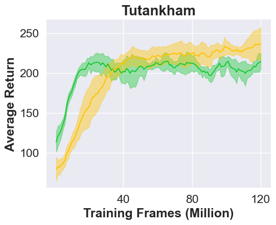
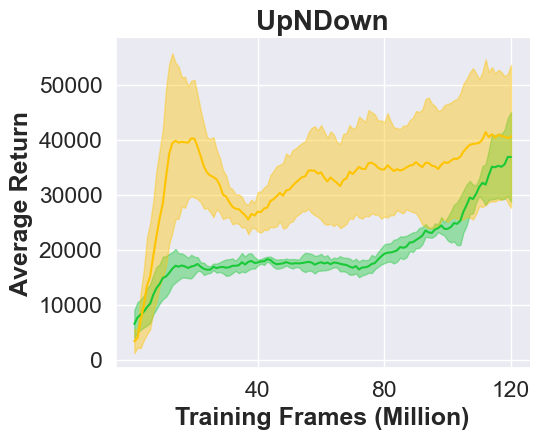
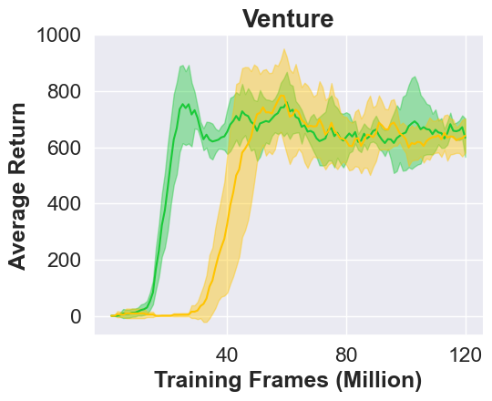
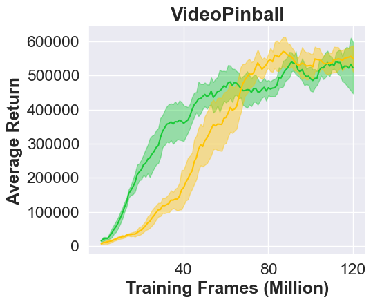
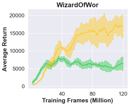
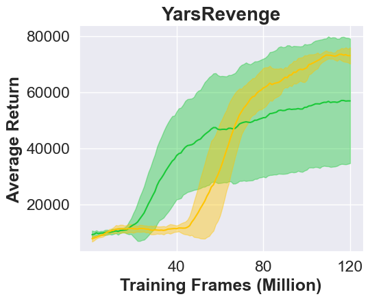
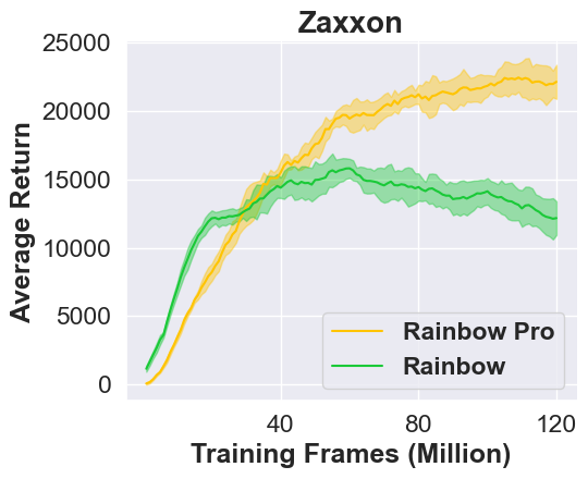
Figure 10: Comparison between Rainbow Pro (yellow) and Rainbow (green) over 55 Atari games (Part II).

12 Motivating Example for Adaptive Updates

In this section we specifically look at 4 domains in which Rainbow Pro did significantly better than the original Rainbow, as well 4 domains where Rainbow Pro is underperforming Rainbow. Note, again, that it is uncommon for Rainbow Pro with the original $\tilde{c}$ to underperform, but here we have a deeper dive into these cases for a better understanding.

From Figure 11, we observe that by using a slightly larger value of $\tilde{c}$, which slightly decreases the incentive for online-target proximity, we can recover from the downside, while still maintaining superior performance on games that are conducive to proximal updates. This suggest that, while using a fixed $\tilde{c}$ value is enough to obtain significant performance improvement, adaptively choosing $\tilde{c}$ would provide us with even more reliable improvements when performing proximal updates. In this context, a promising idea would be to hinge on the variance of our gradient updates when setting $\tilde{c}$. We leave this promising direction for future work.

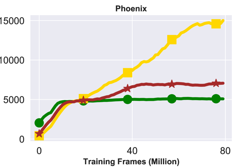
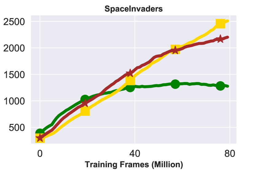
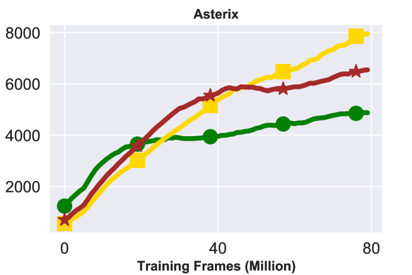
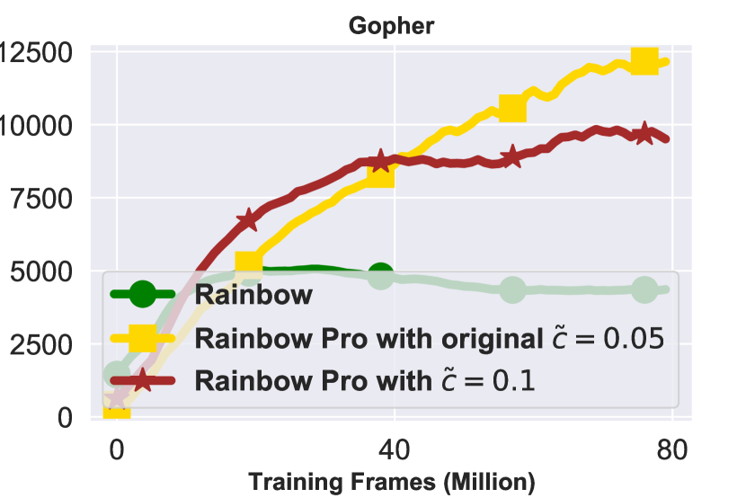
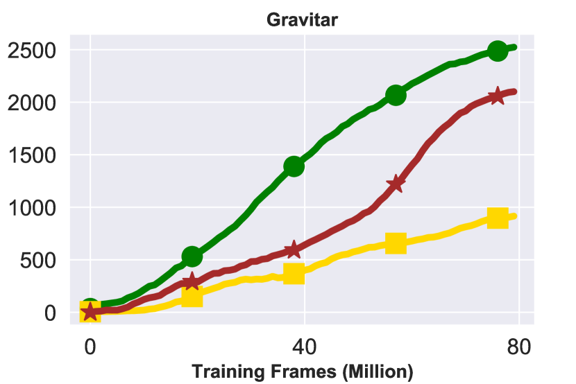
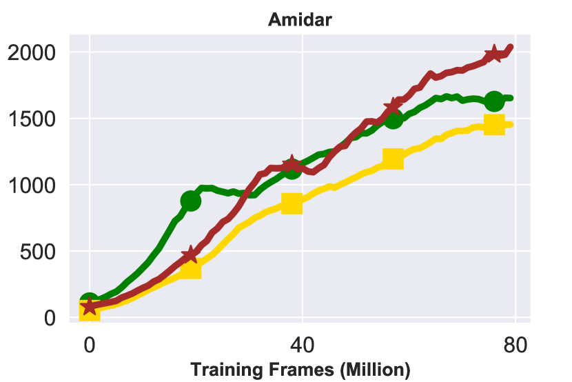
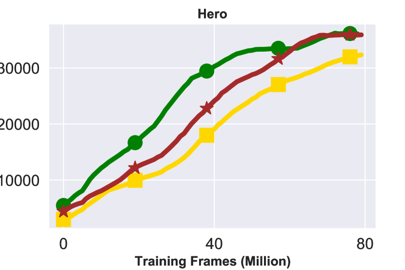
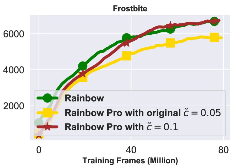
Figure 11: A study on games with the strongest (top) and weakest performance for Rainbow Pro with the original $\tilde{c}=0.05$. Using a slightly less powerful proximal term (corresponding to larger $\tilde{c}=0.1$) enables us to recover the downside (bottom) while still providing benefits on games that are more conducive to using the proximal updates (top).

13 Proximal Updates in the Value Space

Our primary contribution was to show the usefulness of performing proximal updates in the parameter space. That said, we also implemented a version of proximal updates that operated in the value space. More specifically, in this case we updated the parameters of the online network as follows:

$$w\leftarrow\widehat{\text{E}}_{\langle s,a,r,s^{\prime}\rangle}\Big{[}\big{(}r+\gamma\max_{a^{\prime}}\widehat{Q}(s^{\prime},a^{\prime};\theta)-\widehat{Q}(s,a;w)\big{)}^{2}\Big{]}+\frac{1}{\tilde{c}}\widehat{\text{E}}_{\langle s,a\rangle}\Big{[}\big{(}\widehat{Q}(s,a;w)-\widehat{Q}(s,a;\theta)\big{)}^{2}].$$

We conducted numerous experiments using variants of this idea (such as using separate replay buffer for each term, performing the update for all actions in buffered states, etc) but we generally found the value-space updates to be ineffective. As mentioned in the main paper, we believe this is because the parameter-space definition can enforce the proximity globally, while in the value space one can only hope to obtain proximity locally and on a batch of samples. To perform global updates we may need to compute the natural gradient, which typically requires matrix invasion Knight & Lerner (2018), and thus adding significant computational burden to the original algorithm. In comparison, the parameter-space version is effective, simple to implement, and capable of enforcing proximity globally due to the Lipschitz property of neural networks.

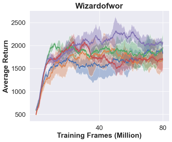
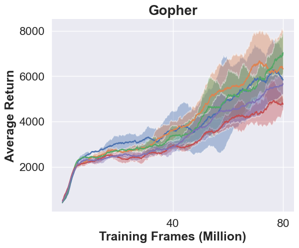
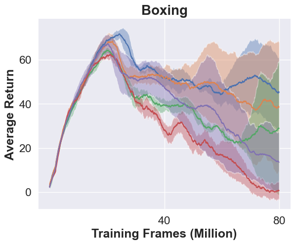
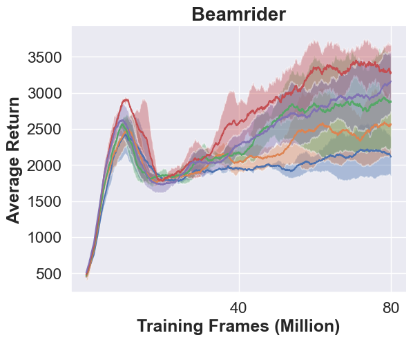
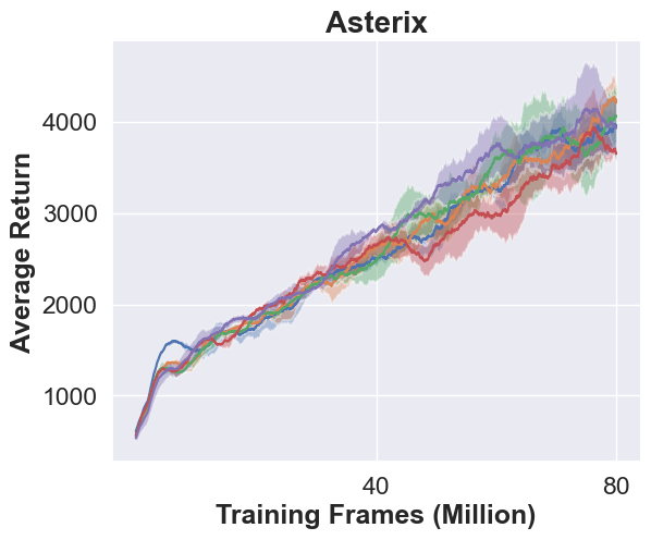
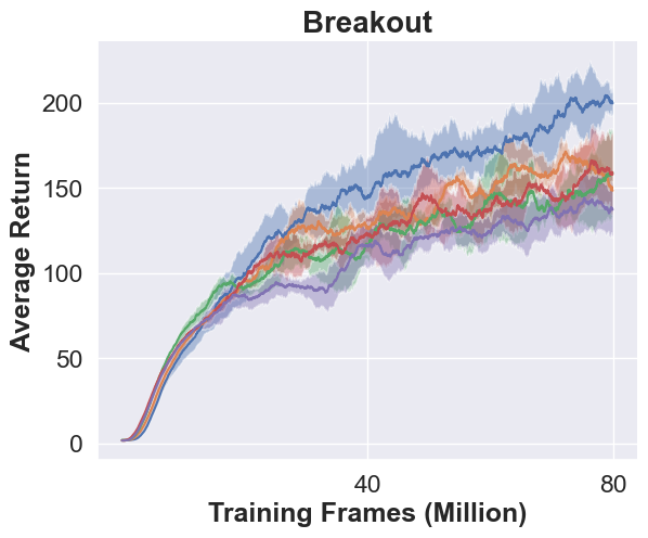
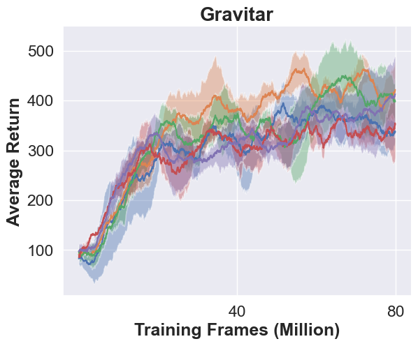
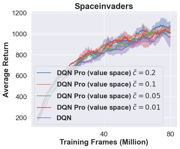
Figure 12: Performing proximal updates in the value space has a limited positive impact.

References

- Arjovsky et al. (2017) Arjovsky, M., Chintala, S., and Bottou, L. Wasserstein generative adversarial networks. In ICML, 2017.
- Asadi et al. (2018) Asadi et al. Lipschitz continuity in model-based reinforcement learning. In ICML, 2018.
- Asadi et al. (2021) Asadi, K., Parikh, N., Parr, R. E., Konidaris, G. D., and Littman, M. L. Deep radial-basis value functions for continuous control. In AAAI Conference on Artificial Intelligence, 2021.
- Beck & Teboulle (2009) Beck, A. and Teboulle, M. A fast iterative shrinkage-thresholding algorithm for linear inverse problems. SIAM Journal on Imaging Sciences, 2009.
- Bellemare et al. (2013) Bellemare, M. G., Naddaf, Y., Veness, J., and Bowling, M. The arcade learning environment: An evaluation platform for general agents. Journal of Artificial Intelligence Research, 2013.
- Bellman (1957) Bellman, R. E. Dynamic Programming. 1957.
- Bertsekas (2011a) Bertsekas, D. P. Incremental gradient, subgradient, and proximal methods for convex optimization: A survey. Optimization for Machine Learning, 2011a.
- Bertsekas (2011b) Bertsekas, D. P. Incremental proximal methods for large scale convex optimization. Mathematical Programming, 2011b.
- Bertsekas & Tsitsiklis (1996) Bertsekas, D. P. and Tsitsiklis, J. N. Neuro-dynamic programming. Athena Scientific, 1996.
- Brockman et al. (2016) Brockman, G., Cheung, V., Pettersson, L., Schneider, J., Schulman, J., Tang, J., and Zaremba, W. Openai gym, 2016.
- Castro et al. (2018) Castro, P. S., Moitra, S., Gelada, C., Kumar, S., and Bellemare, M. G. Dopamine: A Research Framework for Deep Reinforcement Learning. 2018.
- Combettes & Pesquet (2009) Combettes, P. L. and Pesquet, J.-C. Proximal Splitting Methods in Signal Processing. Fixed-point algorithms for inverse problems in science and engineering, 2009.
- Dabney et al. (2018) Dabney, W., Ostrovski, G., Silver, D., and Munos, R. Implicit quantile networks for distributional reinforcement learning. In International conference on machine learning, pp. 1096–1105. PMLR, 2018.
- Fakoor et al. (2020a) Fakoor, R., Chaudhari, P., and Smola, A. J. P3O: Policy-on policy-off policy optimization. In Conference on Uncertainty in Artificial Intelligence, 2020a.
- Fakoor et al. (2020b) Fakoor, R., Chaudhari, P., Soatto, S., and Smola, A. J. Meta-Q-learning. In International Conference on Learning Representations, 2020b.
- Fujimoto et al. (2018) Fujimoto, S., Hoof, H., and Meger, D. Addressing function approximation error in actor-critic methods. In International Conference on Machine Learning, 2018.
- Hessel et al. (2018) Hessel, M., Modayil, J., van Hasselt, H., Schaul, T., Ostrovski, G., Dabney, W., Horgan, D., Piot, B., Azar, M., and Silver, D. Rainbow: Combining improvements in deep reinforcement learning. In AAAI Conference on Artificial Intelligence, 2018.
- Howard (1960) Howard, R. A. Dynamic programming and markov processes. 1960.
- Kim et al. (2019) Kim, S., Asadi, K., Littman, M., and Konidaris, G. Deepmellow: removing the need for a target network in deep q-learning. In International Joint Conference on Artificial Intelligence, 2019.
- Kingma & Ba (2015) Kingma, D. P. and Ba, J. Adam: A method for stochastic optimization. In International Conference on Learning Representations, 2015.
- Knight & Lerner (2018) Knight, E. and Lerner, O. Natural gradient deep q-learning. arXiv preprint arXiv:1803.07482, 2018.
- Kober et al. (2013) Kober, J., Bagnell, J. A., and Peters, J. Reinforcement learning in robotics: A survey. International Journal of Robotics Research, 2013.
- Lee & He (2019) Lee, D. and He, N. Target-based temporal-difference learning. In International Conference on Machine Learning, 2019.
- Li & Lin (2015) Li, H. and Lin, Z. Accelerated proximal gradient methods for nonconvex programming. Advances in neural information processing systems, 2015.
- Lillicrap et al. (2015) Lillicrap, T. P., Hunt, J. J., Pritzel, A., Heess, N., Erez, T., Tassa, Y., Silver, D., and Wierstra, D. Continuous control with deep reinforcement learning. In International Conference on Learning Representations, 2015.
- Lin (1992) Lin, L.-J. Self-improving reactive agents based on reinforcement learning, planning and teaching. Machine learning, 1992.
- Littman & Szepesvári (1996) Littman, M. L. and Szepesvári, C. A generalized reinforcement-learning model: Convergence and applications. In ICML, volume 96, pp. 310–318. Citeseer, 1996.
- Liu et al. (2020) Liu, B., Liu, J., Ghavamzadeh, M., Mahadevan, S., and Petrik, M. Finite-sample analysis of proximal gradient TD algorithms. In Conference on Uncertainty in Artificial Intelligence, 2020.
- Machado et al. (2018) Machado, M. C., Bellemare, M. G., Talvitie, E., Veness, J., Hausknecht, M., and Bowling, M. Revisiting the arcade learning environment: Evaluation protocols and open problems for general agents. Journal of Artificial Intelligence Research, 2018.
- Maggipinto et al. (2020) Maggipinto, M., Susto, G. A., and Chaudhari, P. Proximal deterministic policy gradient. In International Conference on Intelligent Robots and Systems, 2020.
- Mahadevan et al. (2014) Mahadevan, S., Liu, B., Thomas, P., Dabney, W., Giguere, S., Jacek, N., Gemp, I., and Liu, J. Proximal Reinforcement Learning: A New Theory of Sequential Decision Making in Primal-Dual Spaces. arXiv, 2014.
- Martinet (1970) Martinet, B. Regularisation, d’inéquations variationelles par approximations succesives. Revue Francaise d’informatique et de Recherche operationelle, 1970.
- Mnih et al. (2015) Mnih, V., Kavukcuoglu, K., Silver, D., Rusu, A. A., Veness, J., Bellemare, M. G., Graves, A., Riedmiller, M., Fidjeland, A. K., Ostrovski, G., et al. Human-level control through deep reinforcement learning. Nature, 2015.
- Moreau (1962) Moreau, J. J. Fonctions convexes duales et points proximaux dans un espace hilbertien. Comptes rendus hebdomadaires des séances de l’Académie des sciences, 1962.
- Moreau (1965) Moreau, J. J. Proximité et dualité dans un espace hilbertien. Bulletin de la Société Mathématique de France, 1965.
- Nair et al. (2015) Nair, A., Srinivasan, P., Blackwell, S., Alcicek, C., Fearon, R., De Maria, A., Panneershelvam, V., Suleyman, M., Beattie, C., Petersen, S., et al. Massively parallel methods for deep reinforcement learning. arXiv preprint arXiv:1507.04296, 2015.
- Nesterov (1983) Nesterov, Y. A method for unconstrained convex minimization problem with the rate of convergence o (1/k^ 2). In Doklady an USSR, 1983.
- Neyshabur et al. (2015) Neyshabur et al. Norm-based capacity control in neural networks. In COLT, 2015.
- Parikh & Boyd (2014) Parikh, N. and Boyd, S. proximal algorithms. Foundations and Trends in optimization, 2014.
- Polson et al. (2015) Polson, N. G., Scott, J. G., and Willard, B. T. Proximal algorithms in statistics and machine learning. Statistical Science, 2015.
- Puterman (1994) Puterman, M. L. Markov Decision Processes: Discrete Stochastic Dynamic Programming. 1994.
- Reddi et al. (2015) Reddi, S., Poczos, B., and Smola, A. Doubly robust covariate shift correction. In AAAI Conference on Artificial Intelligence, 2015.
- Rockafellar (1976) Rockafellar, R. T. Monotone operators and the proximal point algorithm. SIAM Journal on Control and Optimization, 1976.
- Scherrer et al. (2015) Scherrer, B., Ghavamzadeh, M., Gabillon, V., Lesner, B., and Geist, M. Approximate modified policy iteration and its application to the game of tetris. J. Mach. Learn. Res., 16:1629–1676, 2015.
- Schulman et al. (2015) Schulman, J., Levine, S., Abbeel, P., Jordan, M., and Moritz, P. Trust region policy optimization. In International conference on machine learning, 2015.
- Schulman et al. (2017) Schulman, J., Wolski, F., Dhariwal, P., Radford, A., and Klimov, O. Proximal policy optimization algorithms. arXiv, 2017.
- Silver et al. (2017) Silver, D., Schrittwieser, J., Simonyan, K., Antonoglou, I., Huang, A., Guez, A., Hubert, T., Baker, L., Lai, M., Bolton, A., et al. Mastering the game of go without human knowledge. Nature, 2017.
- Smirnova & Dohmatob (2020) Smirnova, E. and Dohmatob, E. On the convergence of smooth regularized approximate value iteration schemes. Advances in Neural Information Processing Systems, 33, 2020.
- Sutton (1988) Sutton, R. S. Learning to predict by the methods of temporal differences. Machine learning, 1988.
- Sutton & Barto (2018) Sutton, R. S. and Barto, A. G. Reinforcement learning: An introduction. 2018.
- Sutton et al. (2008) Sutton, R. S., Szepesvári, C., and Maei, H. R. A convergent O(n) temporal-difference algorithm for off-policy learning with linear function approximation. In Advances in Neural Information Processing Systems, 2008.
- Tesauro (1994) Tesauro, G. TD-gammon, a self-teaching backgammon program, achieves master-level play. Neural computation, 1994.
- Tomar et al. (2021) Tomar, M., Shani, L., Efroni, Y., and Ghavamzadeh, M. Mirror descent policy optimization, 2021.
- van Hasselt et al. (2018) van Hasselt, H., Doron, Y., Strub, F., Hessel, M., Sonnerat, N., and Modayil, J. Deep reinforcement learning and the deadly triad. arXiv, 2018.
- van Seijen et al. (2019) van Seijen, H., Fatemi, M., and Tavakoli, A. Using a logarithmic mapping to enable lower discount factors in reinforcement learning. Advances in Neural Information Processing Systems, 2019.
- Wang et al. (2019) Wang, Y., He, H., Tan, X., and Gan, Y. Trust region-guided proximal policy optimization. In Advances in Neural Information Processing Systems, 2019.
- Wang et al. (2016) Wang, Z., Schaul, T., Hessel, M., Hasselt, H., Lanctot, M., and Freitas, N. Dueling network architectures for deep reinforcement learning. In International conference on machine learning, pp. 1995–2003. PMLR, 2016.
- Watkins & Dayan (1992) Watkins, C. J. and Dayan, P. Q-learning. Machine learning, 1992.
- Williams et al. (2017) Williams, J. D., Asadi, K., and Zweig, G. Hybrid code networks: practical and efficient end-to-end dialog control with supervised and reinforcement learning. In Association for Computational Linguistics, 2017.
- Zhang et al. (2021) Zhang, S., Yao, H., and Whiteson, S. Breaking the deadly triad with a target network. arXiv, 2021.