A Novel Gaussian Process Based Ground Segmentation Algorithm with Local-Smoothness Estimation

Abstract

Autonomous Land Vehicles (ALV) shall efficiently recognize the ground in unknown environments. A novel $\mathcal{GP}$-based method is proposed for the ground segmentation task in rough driving scenarios. The non-stationary covariance function proposed by [1] is utilized as the kernel for the $\mathcal{GP}$. The ground surface behavior is assumed to only demonstrate local-smoothness. Thus, point estimates of the kernel’s length-scales are obtained. Thus, two Gaussian processes are introduced to separately model the observation and local characteristics of the data. While, the observation process is used to model the ground, the latent process is put on length-scale values to estimate point values of length-scales at each input location. Input locations for this latent process are chosen in a physically-motivated procedure to represent an intuition about ground condition. Furthermore, an intuitive guess of length-scale value is represented by assuming the existence of hypothetical surfaces in the environment that every bunch of data points may be assumed to be resulted from measurements from this surfaces. Bayesian inference is implemented using maximum a Posteriori criterion. The log-marginal likelihood function is assumed to be a multi-task objective function, to represent a whole-frame unbiased view of the ground at each frame. Simulation results shows the effectiveness of the proposed method even in an uneven, rough scene which outperforms similar Gaussian process based ground segmentation methods. While adjacent segments do not have similar ground structure in an uneven scene, the proposed method gives an efficient ground estimation based on a whole-frame viewpoint instead of just estimating segment-wise probable ground surfaces.

I Introduction

In [2] is shown that the efficient ground segmentation task for the sloped terrains needs to be addressed due to consideration of physical-motivated qualities of the data. For the rough scenes, this assumption should be developed more. The technology trends shows more interest in autonomous land vehicles (ALV) with the growth of research interest into the subject. ALV’s are able to provide many opportunities from empowering the ability of remote exploration and navigation in an unknown environment to establishing driver-less cars that are able to navigate autonomously in urban areas being more safe by compensating human driving faults. In order to establish a driver-less car capable of performing autonomously in urban areas, developed methods shall be reliable and real-time implementable. Ground segmentation represents itself as a vital component of any algorithm pursuing further tasks in an unknown environment. A reliable ground segmentation procedure shall be applicable in environments with both flat and sloped terrains, while being realistic and real-time implementable, since often this task is only a prerequisite for other time consuming algorithms and it is an important basic part of ALV’s perception of it’s surroundings. Gaussian process regressions are useful tools for implementation of Bayesian inference which relies on correlation models of inputs and observation data [3]. They provide fast and fully probabilistic framework for non-linear regression problems. Although light detection and ranging (LIDAR) sensors are commonly used in ALVs, data resulted from these sensors, does not inherit smoothness, and therefore, stationary covariance functions may not be used to implement Gaussian regression tasks on these data. Different methods for segmentation have been proposed in the literature [4, 5, 6, 7, 8, 9, 10].

In [4], ground surface is obtained in an iterative routine, using deterministically assigned seed points. In [5], the ground segmentation step is put aside to establish a faster segmentation based on Gaussian process regression. A 2D occupancy grid is used to determine surrounding ground heights, and furthermore, a set of non-ground candidate points are generated. Reference [6] handles real-time segmentation problem by differentiating the minimum and maximum height map in both rectangular and a polar grid map. In [7] a geometric ground estimation is obtained by a piece-wise plane fitting method capable of estimating arbitrary ground surfaces. In [8] a Gaussian process based methodology is used to perform ground estimation by segmenting the data with a fast segmentation method firstly introduced by [9]. The non-stationary covariance function from [1] is used to model the ground observations while no specific physical motivated method is given for choosing length-scales. Paper [10] proposes a fast segmentation method based on local convexity criterion in non-flat urban environments.

These methods are either estimating ground piece-wise and with local viewpoint or by labeling all the individual points with some predefined criterion. Except [8] non of the methods above, gives a continuous model for predicted ground. Furthermore none of them gives an exact, physical motivated routine to extract local characteristics of non-smooth data, while efficient ground segmentation have to be done considering physical realities of the data including non-smoothness of the LIDAR data and ground condition in every data frame.

Due to the ability of Gaussian processes ($\mathcal{GP}$) to model correlations between data points, there is a growth of interest seen in the literature to use them with 3D point clouds. Furthermore, $\mathcal{GP}$s are capable of estimating functional relationships by considering correlations between observations and data points, even when no model is available and the function is prone to huge changes. The correlation is introduced to $\mathcal{GP}$s with covariance kernels. Covariance functions are key concepts in Gaussian process regressions as they define how data points relate to each other. Specification of covariance structures is critical specially in non-parametric regression tasks [11].

LIDAR data is consisted of three-dimensional range data which is collected by a rotating sensor, strapped down to a moving car. This moving sensor obviously causes non-smoothness in it’s measured data, which may not be taken into account using common stationary covariance functions. Although a Gaussian process based method for ground segmentation with non-stationary covariance functions is proposed in the literature to take input-dependent smoothness into account in [8], adjusting covariance kernels to accommodate with physical reality of the ground segmentation problem needs further investigation. Length-scales may be defined as the extent of the area that data points can effect on each other [12]. Length-scale values plays a significant role in the quality of the interpretation that covariance kernel gives about the data. A constant length-scale may not be used with LIDAR data due to non-smoothness of collected point cloud. Different methods are proposed to adjust length scales locally for non-stationary covariance functions by assuming an exact functional relationship for length-scale values [13, 14, 15]. The ground segmentation method proposed by [8] assumes the length-scales to be a defined function of line features in different segments. This is not sufficient because no physical background is considered for the selection of functional relationship and this function might change and fail to describe the underlying data in different locations.

In this paper, two Gaussian processes are considered to jointly perform the ground segmentation task, one to model height of the ground and the other to model length-scale values. A latent Gaussian process is set on the logarithm of length-scale values. Point estimates of length-scale values at each particular ground candidate location is calculated using a multi-task hyper-parameter learning scheme. Local estimation of length-scale values enables the method to consider both flat and sloped terrains. Furthermore, a whole-frame intuition about ground quality of each frame is injected into the optimization task by special treatment of selection process for pseudo-input set. Proposed method is tested on KITTI [16] data set and is shown to outperform similar Gaussian process based ground segmentation methods.

II Radial Grid Map

A radial grid mapping is performed on the LiDAR’s three-dimensional point cloud. The point cloud data is segmented into $M$ different segments. Then each segment is divided into $N$ different bins.

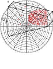
Figure 1: A Two-dimensional Schematic of The Polar Grid Map

The set of all the points in the $n_{th}$ bin of the $m_{th}$ segment is depicted by $P_{b_{n}^{m}}$ which covers the range $(r_{n}^{min},r_{n}^{max})$. In order to reduce the computation effort the set $P_{b_{n}^{m}}^{\prime}$ is constructed that contains the corresponding two-dimensional points:

$$P_{b_{n}^{m}}^{\prime}=\{p_{i}^{\prime}=(r_{i},z_{i})^{T}\;|\;p_{i}\in P_{b_{n}^{m}}\},$$ (1)

where, $r_{i}=\sqrt{x_{i}^{2}+y_{i}^{2}}$ is the radial range of corresponding points. The ground candidate set $PG_{m}$, being the first intuitive guess for obtaining initial ground model is constructed by collecting the point with the lowest height at each bin as the ground candidate in that bin [8]:

$$PG_{m}=\{p_{i}^{\prime}\;|\;p_{i}^{\prime}\in P_{b_{n}^{m}}^{\prime},z_{i}=\min(\mathcal{Z}_{n}^{m})\},$$ (2)

where, $\mathcal{Z}_{n}^{m}$ is the set of height values in $P_{b_{n}^{m}}^{\prime}$. Furthermore, in each bin a vertical segmentation is applied. Each bin is divided into $j$ vertical segments spread from minimum height $z_{min}^{m,n}$ to $z_{max}^{m,n}$. Then the number of points in each of these vertical segments are calculated and averaged on the range to obtain $\tilde{\rho}_{n}^{m}$.

$$\tilde{\rho}_{n}^{m}={\sum_{i=1}^{j}(\rho_{i})}/j$$ (3)

Where $\rho_{i}$ is obtained by dividing the number of points in each vertical segment by the area of that segment.

III Ground Segmentation by Gaussian Process Regression with Local Length-scale Estimate

Gaussian processes ($\mathcal{GP}$) are stochastic processes with any finite number of their random variables being jointly Gaussian distributed. In this paper Gaussian process regression is utilized as a tractable method to put prior distributions over nonlinear function that relates ground model to the radial location of points.

Although $\mathcal{GP}$s are very powerful methods to perform Bayesian inference, they fail to consider non-stationarity and local-smoothness of the data in their general form. In [2] the non-stationarity of the LiDAR point cloud for the ground segmentation task is addressed by using a non-stationary covariance function as the $\mathcal{GP}$s kernel. The length-scales of the proposed kernel is further obtained by a physically-motivated line extraction algorithm which enables the method to perform well both for the flat and sloped terrains.

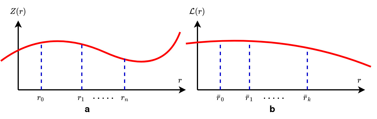
Figure 2: A Schematic of the Two Gaussian Processes. a) The Gaussian process for the ground height estimation b) The Gaussian process for the length-scale estimation.

The LiDAR data also inherits input-dependent smoothness meaning that its data does not bear smooth variation at every part and direction of the environment, thus the stationarity assumption fails to fully describe ground segmentation task. Therefore, covariance functions with constant length-scales are not suitable for LIDAR point cloud since flat grounds must have a larger length-scale than a rough ground.

III-A Problem Definition

Nonlinear Gaussian process regression problem is to recover a functional dependency of the form $y_{i}=f(x_{i})+\epsilon_{i}$ from $n$ observed data points of the training set $\mathcal{D}$. In this paper two different functional dependency is to recover: The ground height $h_{i}=z(r_{i})+{\epsilon_{z}}_{i}$ and the length-scale values $l_{i}=\mathcal{L}(r_{i})+{\epsilon_{l}}_{i}$. The set $PG_{m}\{(r_{i},z_{i})\}$ contains all of two-dimensional ground candidate points in the segment $m$ that the ground model will be inferred based on.

The aim of the algorithm is to obtain the predictive ground model $P(z_{*}|\mathcal{R}_{*},\mathcal{R}_{m},\theta)$:

$$P(z_{*}|\mathcal{R}_{*},\mathcal{R},\theta)=\iint P\big{(}z_{*}|\mathcal{R}_{*},\mathcal{R},exp(\mathcal{L}_{*}),exp(\mathcal{L}),\theta_{z}\big{)}$$

$$P\big{(}\mathcal{L}_{*},\mathcal{L}|\mathcal{R}_{*},\mathcal{R},\bar{\mathcal{L}},\bar{\mathcal{R}},\theta_{l}\big{)}\,dl\,dl_{*}$$ (4)

Where $z_{*}$ represents the ground height prediction at the arbitrary location $r_{*}\in\mathcal{R}_{*}$.The parameter $\mathcal{R}$ represents the training data set. $\mathcal{L}_{*}$ is the mean prediction of the length-scale value at input location $\mathcal{R_{*}}$ and $\mathcal{L}$ is the mean prediction of length-scale at the training data set’s locations. $\theta_{z}$ and $\theta_{l}$ represents the hyper-parameters.

As the marginalization of the predictive distribution of Eq(4) is intractable and Monte Carlo methods are not efficient for the application, the most probable length-scale estimate is obtained:

$$P(z_{*}|\mathcal{R}_{*},\mathcal{R},\theta)=P\big{(}z_{*}|\mathcal{R}_{*},\mathcal{R},exp(\mathcal{L}_{*}),exp(\mathcal{L}),\theta_{z}\big{)}$$ (5)

Since the length-scales are independent latent variables in the combined regression model, making predictions amounts to making two standard $\mathcal{GP}$ predictions. Thus, two separate $\mathcal{GP}$s are assumed to model the ground segmentation task: $\mathcal{GP}_{z}$ and $\mathcal{GP}_{l}$. The $\mathcal{GP}_{z}$ is assumed to model the functional relation of the ground heights with the radial distance of the points with $(\mathcal{L}_{*},\mathcal{L})$ treated as fixed parameters and $\mathcal{GP}_{l}$ is assumed to model the length-scales of the $\mathcal{GP}_{z}$s kernel function. A schematic of these two processes are depicted in the Figure 2.

III-B Problem Formulation

The Gaussian Process for The Ground heights

The $\mathcal{GP}_{z}$ is defined as follows:

$$\mathcal{GP}_{z}:z(r)\sim\mathcal{GP}\big{(}\bar{z}(r),k(r,r^{\prime})\big{)}$$ (6)

With $z(r)$ being the height values at the location $r$, $\bar{z}(r)$ being the mean value of the height at location $r$ and $k(r,r^{\prime})$ being the covariance kernel. Predictive distribution of measurement process can be addressed after obtaining local point estimate of length-scales on locations of ground candidate points. Predictive distribution $P\big{(}z_{*}|\mathcal{R}_{*},\mathcal{R},exp(\mathcal{L}_{*}),exp(\mathcal{L}),\theta_{z}\big{)}$ enables the prediction of $z^{*}$ value at arbitrary locations $r^{*}$ at each point cloud frame:

$$\mu_{\mathcal{GP}_{z}}=\bar{z}=K(r^{*},r)^{T}\bigg{[}K(r,r)+\sigma_{n}^{2}I\bigg{]}^{-1}z,$$ (7)

$$\textrm{cov}_{z_{*}}=K(r_{*},r_{*})-K(r_{*},r)\bigg{[}K(r,r)+\sigma_{n}^{2}I\bigg{]}^{-1}K(r_{*},r)^{T}.$$ (8)

in which, K is the covariance matrix for $\mathcal{GP}_{z}$ and $\sigma_{n}^{2}$ is the measurement noise. The non-stationary covariance kernel from [1] is chosen to represent correlation of measured data points:

$$K(r_{i},r_{j})=\sigma_{f}^{2}.\big{[}\mathcal{L}_{i}^{2}\big{]}^{\frac{1}{4}}\big{[}\mathcal{L}_{j}^{2}\big{]}^{\frac{1}{4}}\big{[}\frac{\mathcal{L}_{i}^{2}+\mathcal{L}_{j}^{2}}{2}\big{]}^{\frac{-1}{2}}$$

$$\times\exp\bigg{(}\frac{-(r_{i}-r_{j})^{2}}{[\mathcal{L}_{i}^{2}+\mathcal{L}_{j}^{2}]}\bigg{)},$$ (9)

where, $\mathcal{L}\in\mathbb{R}$ is length scale for every data point. The predictive distribution of the height $z_{*}$ at the arbitrary test input location $r_{*}$ are obtained using predictive ground model.

Local Length-Scales Estimation

Mean value prediction on latent Gaussian process $\mathcal{GP}_{l}$ results point estimates of length-scale values $\mathcal{L}$. The predictive distribution $P(\mathcal{L}^{*}|\mathcal{R}^{*},\mathcal{R})$ enables point-wise estimation of Length-scale values. regarding to each data point, are calculated by mean prediction of latent process:

$$\mathcal{GP}_{l}:\Rightarrow P(\mathcal{L}_{*}|\mathcal{R}_{*},\mathcal{R})\sim\mathcal{N}(\mathcal{L}_{*},\sigma_{*}^{2}),$$ (10)

$$\mathcal{L}_{*}=\mu_{\mathcal{GP}_{l}}=\log\mathcal{L}=(\bar{K}(r,\bar{r}))^{T}[\bar{K}(\bar{r},\bar{r})+\bar{\sigma}_{n}^{2}I]^{-1}\bar{\mathcal{L}},$$

$$\Rightarrow\mathcal{L}=\exp[(\bar{K}(r,\bar{r}))^{T}[\bar{K}(\bar{r},\bar{r})+\bar{\sigma}_{n}^{2}I]^{-1}\bar{\mathcal{L}}],$$ (11)

in which, $\mathcal{L}^{*}=\mu_{\mathcal{GP}_{l}}$ is the mean value prediction of the logarithm of the length-scale at the desired locations $\bar{R}^{*}$. To obtain length-scale values for each data point, desired locations are adjusted to ground candidate data points at each segment. Matrix $\bar{K}(\bar{r},\bar{r})$ and vector $\bar{K}(r,\bar{r}))$ are corresponding co variances. Furthermore, Covariance parameters for latent process are defined by stationary, squared exponential covariance kernel:

$$\Rightarrow\bar{k}(\bar{r}_{i},\bar{r}_{j})=\bar{\sigma}_{f}^{2}\exp\bigg{(}-\frac{1}{2}\frac{(\bar{r}_{i}-\bar{r}_{j})^{2}}{\bar{\sigma}_{l}^{2}}\bigg{)}.$$ (12)

The $(\bar{\mathcal{L}},\bar{\mathcal{R}})$ is the training set for the length-scale process. These locations of latent kernel are often chosen randomly in the variable space defined by $\mathcal{R}$. In this paper in each segment a pseudo input selection algorithm is performed to obtain these latent training data points.

III-C Pseudo-Input Selection

The input locations for the latent Gaussian process are obtained due to the physical qualities of the ground surface in each segment. A common assumption using LIDAR sensors is that measurements coming from a certain surface must be somehow more related to each other. This assumption yields that if certain area of point cloud data resembles a surface, covariance related characteristics must be similar in that area and differ from other neighboring data points which does not show dependency to the same surface.

Therefore if some measure is introduced for all the points from certain hypothetical surface in point cloud data, this measure can represent a fair measure of length-scale value for that certain area of the data, loyal to the shared surface.

III-D Physically-Motivated Line Extraction

Different line extraction algorithms are being utilized in different robotics applications with some of them being more generally accepted and utilized. Although these algorithms are widely used, some applications need to use different versions of them [8], [17]. Line extraction algorithms are previously used in different ground segmentation methods to enable the distinction of the ground and obstacle points. Thus, although these methods are effective in segmenting near-flat ground points, they fail to properly recognize ground points coming from sloped ground sections or gradient roads. [8] states that despite using a non-stationary covariance function as kernel, their method does not work in the existence of sloped terrains. This can be due to the usage of the Incremental line extraction algorithm which is elaborated in [18] and utilized in [8] to estimate ground surface. The incremental line extraction algorithm lacks the efficiency needed for the detection of sloped terrains. Thus a physically motivated line extraction algorithm along with a two-dimensional line fitting method is introduced which is intuitively compatible with what happens in real-world urban scenarios. The proposed line extraction algorithm relies on the fact that in urban structures, the successive lines of each laser scan should be considered independently. For example, if some structures are found in the data that shows a $3^{\circ}$ slope for a range of radial distance ($2m$) and the algorithm is decided that the last point of this series is a ”critical point”, the parameters of the next line will start to construct from scratch and without dependency to previous segments. This is because the ground candidate points are successive points coming from different bins. Therefore, a sudden change of structure is more important than the overall behavior of some cluster of points as they may be related to a starting point of an obstacle or sloped ground.

Definition of Critical Points

To overcome the problem of sloped terrain detection in the ground segmentation task, the proposed line extraction algorithm operates based on finding some critical points among the ground candidate points set in each segment $PG_{m}$. The critical points are defined to be the points at which the behavior of the successive ground candidate points change in a way that can be flagged as unusual. This unusual behavior happens in the areas that the ground meets the obstacle or as well as the areas at which the road starts to elevate during a slope or gradient section of its. These critical points, therefore, partition each segment into different sections between each two successive critical points. The 2D points between two successive critical points form a line-segment. These line-segments should be chosen carefully as they play a significant role in the line extraction algorithm and the further interpretation of the ground. On the other hand, while large sloped line-segments relate to non-ground structures, the low sloped ones may relate to the ground. Therefore, The conditions listed below must be met for a ground point to be considered as a critical point:

• The slope of fitted line: the slope of the fitted line for the potentially ground-related line segments must be greater than a threshold $\zeta_{b}$.

• Distance from point to the fitted line: distance from points of each line-segment to the fitted line must be less than a given threshold $\delta$.

• Horizontal Distance of the points: The horizontal distance of each two successive points must not exceed a given threshold $\zeta_{m}$. This is set to prevent including breakpoints. This threshold is set concerning each segment and about the radial size of each segment.

• Smoothness of $\tilde{\rho_{n}^{m}}$: The average number of vertical points must not have a sharp change during each line-segment.

Distance-oriented Line Regression

The distance-oriented line regression method is utilized as the core line fitting algorithm. The standard least square method breaks down when the slope of the line is almost vertical or when the slope of the line is large but finite. The least-square method assumes that only the dependent value is subject to error thus the distance of the points to the estimated value $(\hat{y}-y)^{T}(\hat{y}-y)$ is utilized. This assumption makes the algorithm very sensitive to the position of the independent value especially in larger slopes. In these cases, a small inaccuracy in the value of the regressor will lead to greater uncertainty in the value of the regressed parameter if the least square is used as the line fitting algorithm. On the other hand, in many applications such as ground segmentation, this assumption fails to be true as both coordinates are subject to errors. Thus, the least square method is insufficient for sloped terrain ground point detection as the method tends to obtain critical points in areas with larger slopes and the accuracy of detection are of high importance here. The distance-oriented line regression method takes the exact distance of the points to the line into account. The orthogonal least square algorithm is utilized as an alternative for the least square method. The method assumes that both parameters have the same error while this assumption is not valid for line-segment extraction as the 2D value is derived by implementing manipulation on original 3D data. Furthermore, the Non-stationarity assumption of the method denies any similarity of errors in both directions. The mathematical model $\eta=\alpha+\beta\xi$ is assumed to describe the linear relationship of two underlying variables. If both of the variables are observed subject to a random error, the relation of these measurements are as follows:

$$r_{i}=\xi_{i}+\epsilon_{r_{i}}$$ (13)

$$z_{i}=\eta_{i}+\epsilon_{z_{i}}=\alpha+\beta\xi_{i}+\epsilon_{z_{i}}$$ (14)

In which $\epsilon_{r_{i}}\sim\mathcal{N}(0,\sigma^{2})$ and $\epsilon_{z_{i}}\sim\mathcal{N}(0,\lambda\sigma^{2})$. The maximum likelihood estimate for $\alpha$ and $\beta$ is derived. The ”log-likelihood” has the following form:

$$L=-\frac{n}{2}log(4\pi^{2})-\frac{n}{2}log(\lambda\sigma^{4})$$

$$-\frac{\Sigma_{i=1}^{n}(r_{i}-\xi_{i})^{2}}{\sigma^{2}}-\frac{\Sigma_{i=1}^{n}(z_{i}-\alpha-\beta\xi_{i})^{2}}{2\lambda\sigma^{2}}$$ (15)

Differentiating the log-likelihood function with respect to ${\alpha,\beta,\xi,\sigma}$ and solving for $\frac{\partial L}{\partial\star}=0$ yields the numerical estimate of the line parameters.

Figure 3: Ground segmentation results for two different adjacent segments: Red circles represent estimated ground for data points and black squares are the raw data. Blue line is the ground candidate set for each segment.

III-E Learning Hyper–Parameters

The behavior of the proposed model and its ability to adjust itself to physical realities of the environment is directly effected by the values of hyper–parameters. Often in real world applications there is no exact prior knowledge about hyper–parameters value and they must be obtained from data. Hyper–parameters $\theta=\{\sigma_{f},\bar{\mathcal{L}},\sigma_{n},\bar{\sigma}_{f},\bar{\sigma}_{l},\bar{\sigma}_{n}\}$ are mutually independent variables to allow the gradient-based optimization to hold its credibility.

Log Marginal Likelihood: Marginal likelihood or evidence $P(y|\mathcal{X})$ is the integral of likelihood times the prior. Logarithm of marginal likelihood is obtained under Gaussian process assumption that the prior is Gaussian $f|\mathcal{X}\sim\mathcal{N}(0,K)$:

$$\log P(f|\mathcal{X})=-\frac{1}{2}f^{T}K^{-1}f-\frac{1}{2}\log|K|-\frac{n}{2}\log(2\pi)$$ (16)

The maximum a posteriori argument is used to find the hyper–parameters for ground segmentation. The hyper–parameters that maximize the probability of the likelihood of observing $z$ given $R$, are assumed to be valid values for our regression:

$$\log P(\mathcal{L}|z,R,\theta)=$$

$$\log P(z|R,\exp(\mathcal{L}),\theta_{z})+\log P(\mathcal{L}|R,\bar{\mathcal{L}},\bar{R},\theta_{l})$$ (17)

Gradient–based optimization methods are used in order to find the corresponding solutions.

Whole-Frame Objective Function

If optimization process is to be effective enough, it shall take all the segments into account to form an objective function. This would be an example of multi-task regression problem. The objective function in multi-task problems is equal to the sum of all objective functions regarding to different tasks of the problem that share the same hyper-parameters. Therefore, we assume that all the segments share the same hyper–parameters and establish a global view to our frame data in order to have the results to be whole-frame inclusive.

$$L(\theta) = \sum\limits_{m=1}^{M}\bigg{(}\log P(\mathcal{L}^{m}|z^{m},R^{m},\theta)\bigg{)}$$

$$= -\frac{1}{2}\bigg{[}\sum\limits_{m=1}^{M}\bigg{(}(z^{m})^{T}A_{m}^{-1}z^{m}\bigg{)}+\log\bigg{(}\prod\limits_{m=1}^{M}|A_{m}|\bigg{)}$$

$$+ \log\bigg{(}\prod\limits_{m=1}^{M}|B_{m}|\bigg{)}+\log(2\pi)\bigg{(}\sum\limits_{m=1}^{M}(n_{m}+\bar{n}_{m})\bigg{)}\bigg{]}$$

where $A_{m}:=K_{m}(r,r)+\sigma_{n}^{2}I$ and $B_{m}:=\bar{K}_{m}(\bar{r},\bar{r})+\bar{\sigma}_{n}^{2}I$ are the corresponding covariance functions of Gaussian processes in each segment. Therefore, in every segment the ground candidate set with assigned covariance kernels form the segment-wise objective function. Sum of all segment-wised objective functions will form the whole-frame objective function. For the whole-frame objective function to hold its credibility, the hyper-parameters of the regression task must be shared among all segments. Therefore, interpretation of length-scale parameters must be redefined in pseudo-input selection, for all segments to be able to share the hyper-parameter $\bar{\mathcal{L}}$.

Algorithm 1 Line Extraction in segment m

1:INPUT: $M$, $N$, $\zeta_{m}$, $\zeta_{b}$

2:OUTPUT: $PG_{m}$, $L_{m}$

3:$k=0$

4:for  $j=1\;to\;M$  do

5:    for  $i=1\;to\;Size(PG_{m}(j))$  do

6:       if  $P_{b_{n}^{m}}^{\prime}\neq\emptyset$ then

7:          $d_{L}=size(PG_{m}(j))$

8:          if $|d_{L}|\geq 2$ then

9:             $s_{i}=2$

10:             for $n=si\;to\;d_{L}$ do

11:                $(a_{k},b_{k},c_{k})=Fitline(d_{L})$

12:                if  $|\frac{a_{k}}{b_{k}}-\frac{a_{k-1}}{b_{k-1}}|\leq\zeta_{m}$ or $|\frac{c_{k}}{b_{k}}-\frac{c_{k-1}}{b_{k-1}}|\geq\zeta_{b}$  then                 

13:                $s_{i}=n+2$

14:                 goto Line: 10

15:                else

16:                $L_{m}(j)=L_{m}(j)\cup\{a_{k},b_{k},c_{k}\}$                        

17:           $k=k+1$

18:          $d_{L}=\emptyset$            

III-F Gradient Evaluation

The gradients of log marginal likelihood objective function $L(\theta)$ are calculated analytically using,

$$\frac{\partial L(\theta)}{\partial\ast}=\frac{1}{2}\sum\limits_{m=1}^{M}\bigg{(}(z^{m})^{T}A_{m}^{-1}\frac{\partial A_{m}}{\partial\ast}A_{m}^{-1}z^{m}\bigg{)}-$$

$$\frac{1}{2}\sum\limits_{m=1}^{M}\textbf{tr}\bigg{(}A_{m}^{-1}\frac{\partial A_{m}}{\partial\ast}\bigg{)}-\frac{1}{2}\sum\limits_{m=1}^{M}\textbf{tr}\bigg{(}B_{m}^{-1}\frac{\partial B_{m}}{\partial\ast}\bigg{)}$$ (19)

It is then obvious that if we calculate the $\frac{\partial A_{m}}{\partial\ast}$ and $\frac{\partial B_{b}}{\partial\ast}$ for all divided segments, the remaining calculations are found straight forward.

III-G Ground Segmentation Algorithm

The final ground segmentation algorithm is represented in algorithm 2. In every segment m, a candidate two-dimensional ground point set $PG_{m}$ is constructed for every LIDAR frame which can be contaminated by obstacle points as outliers. The typical Gaussian process regression task assumes that all of the data in $PG_{m}$ is ground points with a few outliers. Ground segmentation problem is formulated as obtainment of one regression model with the ability of outlier rejection for each segment in radial grid map, also an iterative learning method is adapted to build the local ground model in every segment which benefits at the same time from both desirable approximation ability and outlier rejection.

Algorithm 2 Ground Segmentation

Input: $P_{t}=\{p_{1},p_{2},...,p_{l}\},M,N,B,\bar{\sigma}_{f},\bar{\sigma}_{n},\bar{\sigma}_{l},\bar{\mathcal{L}}$,
$\sigma_{f},\sigma_{n},\zeta_{g}$
Output: Label of each point $p_{i}\;i=1,2,...,l$

1:$(PG_{m},P_{b_{n}^{m}}^{\prime})=RadialGridMap(P_{t},M,N)$

2:for i = 0 : M-1 do

3:    for j = 0 : Size($P_{b_{n}^{i}}^{\prime}$) do

4:       $L_{j}$ = LineExtraction($P_{b_{n}^{i}}^{\prime}$)

5:       if $Size(PG_{i})>0$  then

6:          ($\bar{y}_{i}$, $\bar{r}_{i}$) = PseudoInputSelection($PG_{i}$)

7:          $\mathcal{L}$ = $GP_{l}$($\bar{r}_{i},\bar{y}_{i},\bar{\sigma}_{f},\bar{\sigma}_{n},\bar{\sigma}_{l},\bar{\mathcal{L}}$)

8:          $\mu_{*}^{l}\leftarrow\mu_{*}^{ij}$ = $GP_{z}$($r_{*},\mathcal{L},\sigma_{f},\sigma_{n}$)            

9:for i = 0 : l  do

10:    if $|z_{i}-\mu_{*}^{i}|>\zeta_{g}$ then label($p_{i}$) = Obstacle

11:    else  label($p_{i}$) = Ground     

This algorithm actually starts with receiving a 3D scan of environment as a set of point clouds $P=\{P_{1},...,P_{k}\}$ which is consisted of $P_{t}$ frames at time $t$ and outputs the label of each point in each point cloud frame as ground or obstacle. The parameter $\zeta_{g}$ represents predefined value for ground loyalty. Points with this height distance from continuous estimation of the ground are considered as obstacle points.

IV Implementation Results

For implementation purposes the input space is divided into $M=180$ different segments covering a 2–degree portion of the environment and each segment is divided into $N=120$ bins. For line extraction purpose $\zeta_{m}$ is set to $0.02$ radians and $\zeta_{b}$ is set to $15^{cm}$, therefore, any line structure with height difference less than $0.15^{m}$ and less than $0.02$ radians deviation from mean angle are assumed to be loyal to a unique line. Regression prediction error is validated using standardized mean squared error by

$$\textrm{SMSE}\equiv\;\frac{1}{n}\sum\limits_{i=1}^{n}\big{[}\textrm{var}(y)^{-1}(y_{i}-\mu_{i})^{2}\big{]}$$ (20)

All the results are obtained on a laptop with Intel Core i7 6700HQ processor and simulations are implemented using point cloud library (PCL) and with C++, while figures are prepared by MATLAB.

Figure 3 shows two different adjacent segments and their ground segmentation result, in which, red circles represent the estimated ground for data points, while black squares are the raw data. As it can be seen in the first row, Figure 3 $a$ and $b$, predicted ground for two adjacent segments have a flat structure, although segment $a$ shows a sloped structure in that area and segment $b$ shows an uneven depth. While the ground candidate set showed in the figure by connected blue line proposes other structure, ground segmentation algorithm predicts a flat ground for this area as a result of considering all the segments together and having a whole-frame. This results shows that general point of view does not obey a segment–wise logic. On the other hand in segments shown in part $c$ and $d$ of this figure, although data in segment $d$ covers a wider region, algorithm tends to estimate detailed structure of ground in both segments regardless of what local ground candidate set may impose based on segment–wise logic. This feature enables the algorithm to truly recognize ground in radial distances ranged from $6$ to $8$, although segment $d$ offers a more smooth ground shape from its data in that range.

Table I: Ground Prediction Results

$n_{PG_{m}}/n_{\mathcal{L}}$	$\sigma_{f}^{2}$	$\sigma_{n}^{2}$	$\bar{\sigma}_{f}^{2}$	$\bar{\sigma}_{l}^{2}$	$\bar{\sigma}_{n}^{2}$	$\textrm{SMSE}_{Z-\mathcal{L}}$	$\textrm{SMSE}_{Z}$	$t_{Z-\mathcal{L}}(s)$	$t_{Z}(s)$
36/23	0.3663	0.8607	1.415e+6	2.250e+6	1.187e+6	2.4258e-27	1.4978e-23	0.5432	0.2335
52/30	0.3117	0.7207	4.729e+6	1.347e+6	2.058e+6	1.2466e-28	1.1231e-23	1.0045	0.4356
68/16	0.4896	1.1544	1.381e+6	3.881e+6	4.501e+6	2.7561e-26	1.4102e-21	0.3283	0.1963
81/14	0.1103	1.6487	4.588e+6	3.521e+6	4.402e+6	4.2903e-19	8.6733e-22	0.2732	0.3412

Furthermore, ground segmentation method of [8] is implemented on the same data. Detailed results of the implementation is given in Table LABEL:table:one. The first two rows are corresponding estimated values for figure 3 $a$ and $b$ with $n_{PG_{m}}/n_{\mathcal{L}}$ being the number of ground candidate points versus number of selected pseudo-input set. It is important to notice that reducing $n_{\mathcal{L}}$ by weakening pseudo-input selection criteria will increase speed of the given algorithm with the expense of reducing the precision. This enables a trade-off between precision and speed of the algorithm. Given results shows that in these two segments, choosing a large pseudo-input set gives a more precise ground estimation result than the other method while making it slower. However it is still real-time applicable and implementable for urban driving scenes. The last two rows are corresponding results for figure 3 $c$ and $d$ while it can be seen that by choosing a small pseudo-input set relating to ground candidate set $14/81$ makes our prediction faster while reduces the precision. This comes from the fact that as the size of pseudo-input set gets larger, the gradient-based optimization step becomes more time consuming. The SMSE. hyper-parameters and time values reported in table LABEL:table:one are recorded for ground segmentation in the corresponding frame while in figure 3 just selected segments are depicted.

As it is seen in these comparison results the proposed method denoted by $Z-\mathcal{L}$ outperforms the conventional method in precision, while being fast enough for urban driving scenarios and robust to the locally changing characteristics of input point cloud. Calculated SMSE error shows that the proposed method is more precise than that of the method given in [8], and its speed is related to the ratio of number of points in pseudo–input set to the number of points in ground candidate set. The SMSE error for each segment is reported as the mean value of 100 iterations of ground prediction. Furthermore, values of hyper-parameters are reported. In order to consider different scales of covariance kernels, while scaled gradient-based optimization method is used to find optimal hyper–parameters.

This real-time applicable ground segmentation procedure may be applied efficiently in applications, where fast and precise clustering and ground segmentation is needed to enable further real-time processes like path planning or dynamic object recognition and tracking especially in rough scenes. Furthermore, taking location-dependent characteristics of non-linear regression into accounts, enables the method to show better performance in rough scenes. In addition, the initial guess of length-scale parameters which is based on fast line extraction algorithm, increases the time efficiency of the proposed method by providing physical motivated initial guess for the $\bar{\mathcal{L}}$ vector. Furthermore, the physical motivated procedure of choosing each segment’s length-scale vector, gives the method a sense of intuition which is related to the ground quality. This intuition which is behind choosing the most important parameters of the regression method, ensures the fair calculation of ground at each individual frame with respect to its specifications.

V Conclusions

A physically-motivated ground segmentation method is proposed based on Gaussian process regression methodology. Non-smoothness of LIDAR data is introduced into the regression task by choosing a non-stationary covariance function represented in equation III-B for the main process. Furthermore, local characteristics of the data is introduced into the method by considering non-constant length-scales for these covariance function. A latent Gaussian process is put on the logarithm of the length-scales to result a physically-motivated estimation of local characteristics of the main process. A pseudo-input set is introduced for the latent process that is selected with a whole-frame view of the data and based on the ground quality of the data in each segment by assuming the related correlation of data points that are gathered from same surface.

It is verified in this paper that the proposed method outperforms conventional methods while being realistic, precise and real-time applicable. Furthermore, presented results shows that proposed method is capable of effective estimation of the ground in rough scenes. While the ground structure in the given example in figure 3 may be assumed to be rough as it contains bumpy structures and sloped obstacles, the proposed method is capable to detect ground model efficiently and precisely.

References

- [1] C. J. Paciorek and M. J. Schervish, “Nonstationary Covariance Functions for Gaussian Process Regression,” pp. 1–27, 2003.
- [2] H. D. T. Pouria Mehrabi, “A Gaussian Process-Based Ground Segmentation for Sloped Terrains,” IEEE Int. Intell. Veh. Symp., 2021.
- [3] C. W. C.E. Rasmussen, Gaussian Processes for Machine Learning. MIT Press, 2006.
- [4] D. Zermas, I. Izzat, and N. Papanikolopoulos, “Fast Segmentation of 3D Point Clouds : A Paradigm on LiDAR Data for Autonomous Vehicle Applications,” IEEE Int. Conf. Robot. Autom., no. May, pp. 5067–5073, 2017.
- [5] M.-O. Shin, G.-M. Oh, S.-W. Kim, and S.-W. Seo, “Real-Time and Accurate Segmentation of 3-D Point Clouds Based on Gaussian Process Regression,” IEEE Trans. Intell. Transp. Syst., pp. 1–15, 2017. [Online]. Available: http://ieeexplore.ieee.org/document/7895118/
- [6] D. Korchev, S. Cheng, Y. Owechko, and K. Kim, “On Real-Time LIDAR Data Segmentation and Classification,” Worldcomp-Proceedings.Com, no. February, 2016. [Online]. Available: http://worldcomp-proceedings.com/proc/p2013/IPC2940.pdf
- [7] A. Asvadi, C. Premebida, P. Peixoto, and U. Nunes, “3D Lidar-based static and moving obstacle detection in driving environments: An approach based on voxels and multi-region ground planes,” Rob. Auton. Syst., 2016. [Online]. Available: http://dx.doi.org/10.1016/j.robot.2016.06.007
- [8] T. Chen, B. Dai, R. Wang, and D. Liu, “Gaussian-Process-Based Real-Time Ground Segmentation for Autonomous Land Vehicles,” J. Intell. Robot. Syst. Theory Appl., vol. 76, no. 3-4, pp. 563–582, 2014.
- [9] M. Himmelsbach, F. von Hundelshausen, and H. Wuensche, “Fast segmentation of 3D point clouds for ground vehicles,” IEEE Int. Intell. Veh. Symp., pp. 560–565, 2010.
- [10] F. Moosmann, O. Pink, and C. Stiller, “Segmentation of 3D lidar data in non-flat urban environments using a local convexity criterion,” IEEE Intell. Veh. Symp. Proc., pp. 215–220, 2009.
- [11] M. Stein, “Nonstationary spatial covariance functions,” Unpubl. Tech. report. Available, vol. 60637, pp. 0–7, 2005. [Online]. Available: http://www-personal.umich.edu/ jizhu/jizhu/covar/Stein-Summary.pdf
- [12] C. Plagemann, K. Kersting, and W. Burgard, “Nonstationary Gaussian process regression using point estimates of local smoothness,” Lect. Notes Comput. Sci. (including Subser. Lect. Notes Artif. Intell. Lect. Notes Bioinformatics), vol. 5212 LNAI, no. PART 2, pp. 204–219, 2008.
- [13] Y. Zhang and G. Luo, “Recursive prediction algorithm for non-stationary Gaussian Process,” J. Syst. Softw., vol. 127, pp. 295–301, 2017. [Online]. Available: http://dx.doi.org/10.1016/j.jss.2016.08.036
- [14] G.-A. Fuglstad, F. Lindgren, D. Simpson, and H. Rue, “Exploring a new class of non-stationary spatial Gaussian random fields with varying local anisotropy,” arXiv, vol. 25, no. 1, pp. 1–28, 2013. [Online]. Available: http://arxiv.org/abs/1304.6949
- [15] G. A. Fuglstad, D. Simpson, F. Lindgren, and H. Rue, “Does non-stationary spatial data always require non-stationary random fields?” Spat. Stat., vol. 14, pp. 505–531, 2015.
- [16] A. Geiger, P. Lenz, C. Stiller, and R. Urtasun, “Vision meets robotics: The KITTI dataset,” Int. J. Rob. Res., vol. 32, no. 11, pp. 1231–1237, 2013. [Online]. Available: http://ijr.sagepub.com/cgi/doi/10.1177/0278364913491297
- [17] A. Siadat, A. Karke, S. Klausmann, M. Dufaut, and R. Husson, “An Optimized Segmentation Method for a 2-{D} Laser Scanner Applied to MobileRobot Navigation,” Proc. 3rd IFAC Symp. Intell. Components Instruments forControl Appl., no. JULY 1999, pp. 153–158, 1997.
- [18] V. Nguyen, A. Martinelli, N. Tomatis, and R. Siegwart, “A comparison of line extraction algorithms using 2D laser rangefinder for indoor mobile robotics,” pp. 1929–34, 2005.