Bright and Dark States of Light: The Quantum Origin of Classical Interference
Abstract
According to classical theory, the combined effect of several electromagnetic fields is described under the generic term of interference, where intensity patterns with maxima and minima emerge over space. On the other hand, quantum theory asserts that considering only the expectation value of the total field is insufficient to describe light-matter coupling, and the most widespread explanation highlights the role of quantum fluctuations to obtain correct predictions. We here connect the two worlds by showing that classical interference can be quantum-mechanically interpreted as a bosonic form of super- and subradiance, giving rise to bright and dark states for light modes. We revisit the double-slit experiment and the Mach-Zehnder interferometer, reinterpreting their predictions in terms of collective states of the radiation field. We also demonstrate that quantum fluctuations are not the key ingredient in describing the light-matter quantum dynamics when several vacuum modes are involved. In light of our approach, the unambiguous criterion for the coupling to occur is the presence of non-dark states when decomposing the collective state of light. We discuss how the results here discussed could be verified in trapped ion systems or in cross-cavity setups. Finally, we show how the bosonic bright and dark states can be employed to implement quantum gates, which paves the way for the engineering of multimode schemes for universal quantum computing.
I Introduction
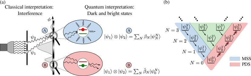
Interference phenomena are fundamental to understanding how electromagnetic waves combine in our environment to eventually interact with matter. If one considers two electromagnetic waves with the same polarization, with complex electric fields and at the position of an atom with an electric dipole moment, the resulting total field reads . Consequently, interference is said to be constructive for in-phase fields and destructive for out-of-phase fields (see Fig. 1(a)). This reflects the importance of the relative phase of the electric field for the atom-light coupling, since the atom can experience an amplified, or diminished, total field due to this interference pattern.
The advent of quantum optics brought new fundamental insights on how light interacts with matter. According to this theory, the picture of a dipole moment generated by an average electric field is incomplete, when not completely wrong. Indeed, even when one considers a single light mode coupled to the particle, a Fock state yields for any number of photons , but it does generate non-trivial light-atom dynamics. The most accepted solution to this conundrum, supported by quantum optics textbooks [1, 2, 3, 4], argues that Fock states possess an electric field variance , which is nonzero, even for the vacuum state (). This sounds reasonable since, as any observable in quantum mechanics, the electric field is fully described only when considering all of its moments . Classical optics addresses the lowest moment (), with all higher moments which are intrinsically given by . Quantum-mechanically, this corresponds to a coherent state in the limit of large photon numbers [5].
In this context, the concept of interference which describes the summation of fields in classical optics has little relevance; if classical optics fails to describe the coupling of a particle to a single-mode Fock state, how could it properly describe the combination of several such modes? This highlights an important gap in the classical understanding for the summation of fields, and their joint interaction with matter. While the concept of interference presents a rather intuitive picture in the classical world, no clear equivalent exists to describe the summation of quantum fields.
In this work, we bridge this gap by showing that a decomposition of the total state of the radiation field on a collective Dicke-like bosonic basis offers a natural interpretation of constructive and destructive interferences, in terms of bright (or superradiant) and dark (or subradiant) states. Using this framework, we prove that quantum fluctuations are not the key ingredient to explain the light-atom coupling. The necessary and sufficient condition instead is the existence of at least one finite projection on a non-dark state. Furthermore, the collective basis for bosonic modes predicts a vast class of entangled states which couple to the atom with intermediate superradiant transition rates, with no counterpart in classical theory.
The manuscript is organized as follows: In Sec. II, we introduce the collective basis, with a particular attention to perfectly dark and maximally superradiant states. In Sec. III, we discuss how these states relate to destructive and constructive interference in classical theory. We also discuss why classical interference is unable to properly describe the excitation of an atom, whereas our approach provides a natural explanation. In Sec. IV, we revisit the double-slit experiment using the collective basis. Then, in Sec. V, we discuss the different interference patterns obtained in a Mach-Zehnder interferometer when employing quantum and classical fields, interpreting the results in terms of collective states. In Sec. VI, we extend our formalism to modes and, in Sec. VII, we discuss how our predictions could be observed using trapped ions or cavity QED setups. Application of dark and bright states in quantum information processing is presented in Sec. VIII. The conclusions and perspectives are presented in Sec. IX, and a detailed derivation of the analytical expressions presented in the main text can be found in the Appendices.
II Two-mode collective basis
Let us consider two light modes and , with annihilation (creation) operators () and (), coupled resonantly to a two-level atom. The raising (lowering) atomic operator () realizes transitions between ground and excited states, and the coupling constant is assumed identical for both modes, for simplicity. Such an atom-modes system is described by the following Hamiltonian in the interaction picture:
| (1) |
The dimensionless total electric field operator at the atom position is given by the superposition of the two fields:
| (2) |
The atom acts as a probe for the field resulting from the combination of the fields at its position. Yet, as we shall see later, the particle may not be excited even by a nontrivial field, in which case other ways are required to detect the state of the fields (see Sec. VII). From a classical point of view, all operators in (2) must be replaced by complex amplitudes, and the atom is not excited only if the total electric field is zero. Quantum mechanically, as discussed in the introduction, the atom can be excited by light modes with zero electric field expectation value (such as Fock states), a phenomenon attributed to the quantum fluctuations of the field. Yet, it turns out that there exist two-mode fields with nonzero quantum fluctuations, other than the vacuum, which do not excite the atom. Hence, quantum fluctuations cannot be the only explanation of why the emitter is excited by a superposition of light modes
Let us illustrate the apparent inconsistency between the coupling of combined fields with matter in the classical and quantum pictures. To this end we first consider the coherent states and in the modes and . Using the eigenvalue relations and , we obtain
| (3) |
making clear that the state is unable to excite the atom. This can be explained invoking classical interference, since the sum of the nonzero expectation values of the electric field from each mode actually cancels out:
| (4) | |||||
However, such an explanation fails for the state
| (5) |
which also has a zero total electric field expectation value, but survives the action of the Hamiltonian: . Therefore, the atom-field coupling does not cancel for state .
As pointed out in the introduction, quantum fluctuations would be the next natural candidate to explain why two different states with affect the atom in such disparate ways. However, the scenario becomes even more puzzling when we compute the variance of for the states and : it gives for both cases, which is the same as the two-mode vacuum state. Therefore, the two states here presented with exhibit nonzero quantum fluctuation, yet only is able to excite the atom. These simple examples naturally lead us to the following question: Why do some states of the radiation field couple to matter, and others do not? If the explanation is not the average field and fluctuations, then what is the proper criterion for such a coupling to occur?
To address this question, we introduce the following set of two-mode -photon states:
| (6) |
where refers to the product Fock state with photons in mode and in mode . The coefficients of these collective states are given by (see Appendix A)
with and . States (6) are derived from the symmetric and antisymmetric collective operators [6, 7], and constitute a complete basis which satisfies the following coupling relation:
| (8) |
The physical process described by (8) corresponds to the excitation of the atom through the transition from state to , see Fig. 1(b).
The collective basis (6) presents a strong analogy to the -excitation Dicke basis for multi-atom systems [8, 9]. In analogy to the “cooperation number” for Dicke states, the factor represents the cooperativity of the emission, where the factor comes from the fact that there are two modes interacting with the atom. In particular, the case corresponds to the perfectly dark state (PDS) for the subspace of photons
| (9) |
which does not couple to the atom. It was coined subradiant by Dicke since . Oppositely, the state
| (10) |
presents a transition rate , which is times that of the single-mode result: [10], with the Jaynes-Cummings Hamiltonian. State (10) is the analogue of the symmetric superradiant mode, studied by Dicke in the decay cascade [8, 11], and represents the most superradiant of the states with photons. We here refer to this state as the maximally superradiant state (MSS). Finally, states within the range present intermediate transition rates. As opposed to the two-level atom case, the present Hilbert space is unbounded, even for a finite number of field modes, since each one can support an arbitrary number of photons [9], see Fig.1(b).
III Connection with classical interference
Let us now discuss how this basis articulates with the concept of interference, starting with two-mode coherent states. When considering in-phase coherent states, one obtains a state that decomposes exclusively on the MSS subspace:
| (11) |
This implies that the emission is enhanced by a factor 2 as compared to a single coherent state: against , respectively. This result is here interpreted as the signature of a state which projects on the MSS subspace only, but from a classical perspective, it corresponds to a constructive interference for in-phase fields. As for the state describing two coherent fields with opposite phases, it decomposes in terms of PDSs only:
| (12) |
This state presents a suppressed interaction , which can be interpreted either as belonging to the PDS subspace or, classically, as a destructive interference for two fields with the same amplitude, but opposite phases.
Less intuitively, the introduced basis provides an explanation for the coupling of state from Eq. (5) to the atom, despite it having zero average electric field (a destructive interference from the classical perspective) and the same electric field variance as state . Indeed, it decomposes along MSS and PDS subspaces as
| (13) |
so the finite projection on the MSS is responsible for the nontrivial action of the Hamiltonian.
The PDS subspace is a remarkable class of states. On the one hand, from a classical perspective, destructive interference is considered an absence of field, which explains the absence of a generated dipole moment. On the other hand, fluctuations in the electric field operator are usually invoked to explain the excitation of an atom in the absence of a field expectation value, as illustrated by the emblematic single-mode Fock states. Perfectly dark states are transverse to these characteristics since they possess nonzero fluctuations (, see Appendix B), an energy proportional to their photon number , and yet they do not excite the atom. In other words, they go beyond the classical interpretation of destructive interference, for which the fields simply cancel out.
Naturally, a coherent state in only one of the two modes does not provide any collective feature: . In the collective basis, it decomposes as
| (14) |
which is a combination of modes of various transition rates, averaging out as the transition rate of a single coherent mode. The situation is equivalent to that of two atoms with a single one excited, , which decomposes equally on the superradiant [] and subradiant [] states as . Therefore, its radiation averages into the single-atom one.
IV Revisiting the double-slit experiment
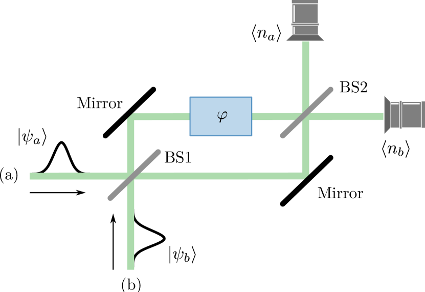
A key experiment in evidencing the wave nature of light is the Young slit experiment or, equivalently, the Mach-Zehnder interferometer. The fundamental result is that both classical and single-photon coherent sources produce the same fringe pattern, despite the very different natures of these fields, and despite the latter source is composed of a single quantum of energy. To revisit this experiment using the collective basis, one can consider, in the far field limit, two equal-weight light modes, as previously. Without loss of generality, we assume that the waves with wave vectors and , with , reach the two slits with the same phase. Then, and are the phases acquired by the respective fields when propagating from slits 1 and 2, respectively, until the detection point (see Fig. 1).
For modes in coherent states, the field on the detector writes
| (15) |
whereas for single-photon states
| (16) |
where represents the phase difference due to the distinct light paths until the detector. In Eq. (15), we have defined the phase-dependent state
| (17) |
which corresponds to a MSS when the two modes are in phase, , and to a PDS when in opposite phases, , with . The single-photon state , which decomposes as a sum of PDS or MSS only [see Eq. (16)], presents the same feature. Therefore, the decomposition in PDSs and MSSs straightforwardly explains why single-photon sources and classical fields exhibit the same fringe pattern, for a ground state atom. The particular case of the slits actually points toward a more general result: states of light composed of PDSs and MSSs only exhibit the same interference patterns as those derived from linear optics or, equivalently, for high-photon-number coherent states.
V Mach-Zehnder interferometer (MZI)
To pursue the discussion on the detection of light states of different natures, let us now consider the MZI setup with two input fields which are either classical fields, with Rabi frequencies and , or quantum fields which belong to the PDS subspace, or to the MSS subspace. The latter can be written in terms of creation operators as (see Appendix A). For classical (quantum) fields, corresponds to the case of constructive interference (MSSs only), and to destructive interference (PDSs only). For either kind of state, the output intensity is (see Appendix C)
| (18) |
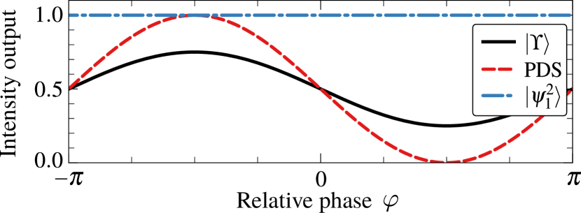
where refers to the arm , is the intensity of the input field and the relative phase shift between the two arms of the interferometer. Eq. (18) shows that classical and quantum fields exhibit the same fringe pattern through MZI as the phase is varied. Differently, state has a projection on both MSS and PDS subspaces and it leads to the following output in the MZI:
| (19) |
This fringe pattern is qualitatively different from the one obtained for classical fields, and for pure PDSs or MSSs, since the intensity does not cancel. Its minimum is , with a visibility
| (20) |
which is half the value of obtained for classical states and PDS-only or MSS-only. This finite minimum of the intensity can be interpreted in terms of the Hong-Ou-Mandel effect [1, 2], where the projection of on the two-indistinguishable-photon state automatically leads to a nonzero intensity in the MZI.
According to our predictions, PDSs and MSSs provide the same signatures as classical fields through interferometric setups, despite their quantum nature – the states which compose the PDS and MSS basis are photon-number states. Combined with the fact that the “classical” state (or ) decomposes as MSSs (or PDSs) only, this shows that the collective basis offers a natural frame for the concept of interference. Independently of the (classical or quantum) nature of the light, MSSs and arbitrary combinations of them correspond to constructive interference, whereas PDSs result in destructive interference. While for the other states, such as , more elements from the collective basis are necessary to properly assess their coupling to matter.
Our collective basis (6) reveals a broad family of “intermediate” states, which are neither perfectly dark nor maximally superradiant ( for ). By injecting such states in the MZI, one obtains interference patterns which cannot be described by classical theory. For instance, considering the input (entangled) state , the output in arm is , independently of the relative phase of the MZI (see Appendix D). In this case, the fringes have completely disappeared, and the visibility is zero. In Fig. 2, we plot the output intensity in arm as a function of the phase , which highlights the qualitative difference between the different states of light considered. Note that while the PDS considered here is a combination of two out-of-phase coherent (classical) fields, any PDS will provide the same interference pattern, whether classical or quantum. Differently, states and present patterns that are different from those obtained with classical states, where the intensity cancels. In this sense, the reduction of visibility here stems from the quantum nature of the field.
Inspired by the collective basis, let us now introduce a protocol to identify the nature of the light field. As a slight alteration of these setups, we now consider an atom in the excited state to locally probe the field. In this case, two classical fields with the same amplitude, but with opposite phase, do not act on the atom since the classical Hamiltonian simply cancels. Alternatively, a quantum field with a small average number of photons, even in a superposition of PDSs, does exchange energy with the atom. This can be easily demonstrated using the evolution operator , with given by Eq. (1), and by noticing that any superposition of PDSs can be written as (see Appendix A). Using the commutation relation , one obtains
| (21) |
which, in general, is nonzero. Hence, PDSs exchange energy with an atom in the excited state, just as the two-mode vacuum state does. Thus, the slit experiment combined with a two-level emitter as a probe appears as a new tool to probe the nature of the probe field. This makes field-field correlations appropriate tools to probe the quantum nature of light, instead of the usual intensity-intensity correlations [1, 2]. From a fundamental point of view, this difference between few- (quantum) and many-photon (classical) fields stems from the difference between classical and quantum vacuum. In essence, it is related to the non-commutation relation between and , which implies that the addition and then the subtraction of a photon differs completely from the subtraction followed by the addition of a photon [12, 13].
The similarities between the “true” vacuum state and PDSs raises the question of whether it is possible to distinguish the two, since neither a ground-state nor an excited-state atom can differentiate them. However, it is sufficient to observe that a change in the balance between the two modes (not achievable in free space, where the atom-field coupling is very small) would immediately change the nature of the mode (provided it is not the vacuum state), giving the new mode a nonzero projection onto bright states. For example, in a two-mode cavity, taking into account the transverse shape of the modes means that a transverse displacement of the emitter would allow for the atom to radiate, as long as the two cavities are not in the vacuum state. In particular, such an experiment could help investigate the existence of a “dark-like energy”, since PDSs have an energy proportional to their number of photons (in addition to the energy of the true vacuum state), yet no coupling to the matter. Note that the discussion on the coupling of an atom with a field which locally cancels is reminiscent of the finite momentum diffusion for an atom at the crossing of two lasers, where the fields interfere destructively. The existence of heating is, in that case, related to the spatial gradient of the field, rather than to its quantum fluctuations [14, 15].
VI Generalization to modes
Let us now discuss how our approach generalizes to an arbitrary number of light modes. For modes equally coupled to the atom, the interaction Hamiltonian reads:
| (22) |
with () the annihilation (creation) operator for the th light mode. Then, the following generalized coupling relation can be derived (see Appendix E):
| (23) |
where we have defined the collective -mode basis
| (24) |
for the subspace of photons. In Eq.(24), we define the orthogonal matrix of dimension , with even, whose elements in the first row are , while the elements in the second row satisfy the rule (see Appendix E). Consequently, we identify the MSSs as
| (25) |
associated with the largest transition rate . The anti-symmetric PDSs read
| (26) |
As for the two-mode case, we are now able to expand the -mode in-phase coherent state in terms of MSSs only:
| (27) |
which leads to the coupling relation . Therefore, the exchange of energy between the atom and the modes in coherent states is times faster than the case of a single cavity mode. Finally, the -mode coherent state corresponding to destructive interference decomposes in the PDS subspace only:
| (28) |
implying immediately the dark state condition .
Considering the more general case of modes, one can now identify that the single mode case () presents a unique PDS, namely, the vacuum state . This case may sound trivial since there is no photon to excite the atom, yet its interest lies in its unicity: any other state excites the atom. The multimode case is fundamentally different since it possesses an infinite family of dark states, with arbitrarily high photon numbers, yet which do not couple to the emitter in the ground state. This scenario is analogous to the case of two-level atoms, where the single-atom (spontaneous) emission always occurs, whereas the emission from a couple of atoms is suppressed in their dark state . In this context, the collective basis is the natural frame to understand why single-mode Fock states couple to matter (since they do not belong to the PDS subspace), whereas two-mode PDSs states with quantum fluctuations do not. Alternatively, dark states can be produced using single emitters with a multilevel structure [16], in particular in Electromagnetically Induced Transparency [17].
VII Detection scheme
The two-mode or -mode light-matter interaction discussed in the present work suggests an implementation in setups where the electromagnetic environment is reduced to a few modes. Examples are optical cavities coupled to a two-level atom [18, 19], trapped ions where a single emitter can be coupled to its two vibrational modes [20, 21], or superconducting circuits [22]. We point out that an important example of the present discussion is the case of two coherent states with the same photon number but opposite phases; these light modes possess nonzero quantum fluctuations, but do not couple to the emitter. A crossed detection of the atom dynamics (for example, from its fluorescence) coupled to a detection of the statistics of the cavity modes, would allow unambiguous measurement of the features discussed in this work. Note that the cavity’s finite finesse (and thus nonzero cavity decay rate) and the atom’s spontaneous emission (atomic decay rate) are not expected to affect these features, since they are purely diagonal terms.
We study the dynamics of the atom coupled to two cavity modes using a quantum master equation, which takes into account the atom and mode dissipation:
| (29) |
with and , with , and where and are the atomic and field decay rates, respectively. This master equation is the standard one employed to study atom-cavity dynamics and is valid under the Rotating Wave Approximation (RWA), where the atom-field coupling energy is much smaller than the free energy of the modes and of the atom, and Born and Markov approximations [2].
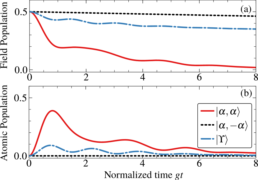
Considering an intermediate () or strong () atom-field coupling, the results predicted in this work could be observed by monitoring the modes and atomic populations, see Fig. 3. Starting with the atom in the ground state , state exchanges energy with the atom while the state does not. On the other hand, state excites the atom despite its zero average electric field, and electric field fluctuations equal to those of the states. Thus, by monitoring the excited atomic state population one could distinguish the states considered here, see Fig. 3(a). One could also observe the atom-field coupling/non-coupling by monitoring the cavity mode emission, since the atom acts as an extra source of decay for the cavity modes (that is, for the states which couples to the atom), with an effective decay rate [23, 24]. In Fig. 3(a) we plot the average number of photons in the cavity mode (which is the same as in mode ), which shows that the cavity emission depends on the mode state, as expected. In particular, the state remains completely unaffected by the presence of the atom.
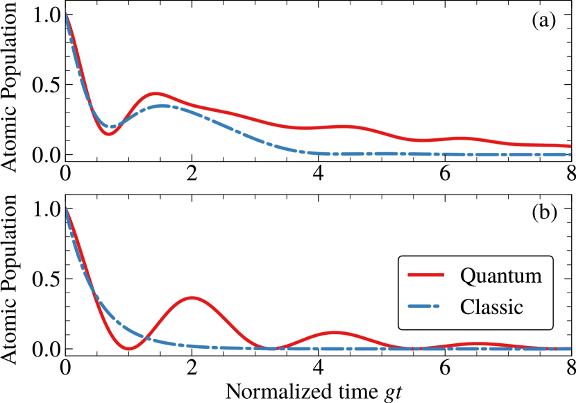
Let us now discuss further how the interference experiment presented in Sec. V allows one to distinguish PDSs from classical fields, provided a two-level detector in the excited state is used. In Fig. 4, considering an atom initially in the excited state , we present the evolution of the excited state population for different field states, described by either a quantum model, derived from Eq. (29), or a semi-classical one. The latter is obtained by deriving from Eq. (29) the equations of motion for the atomic and the cavity field operators. Then, the expected value for the collective operator of the radiation field is replaced by time-dependent complex amplitude (see Appendix F for details). The panels (a) and (b) in Fig. 4 describe, respectively, in-phase ( and , for quantum and semi-classical models, respectively) and out-of-phase ( and , for quantum and semi-classical models, respectively) fields, and they exhibit a qualitative difference between the two approaches. One observes that the semi-classical model predicts a monotonic decay, while the quantum one predicts an oscillating decay: this shows that a quantum and a classical field can be distinguished with this protocol.
VIII Application: Controlled-Phase Gate
One can take advantage of the bright and dark states of the cavity modes for quantum information processing. To illustrate this point, let us now present how to implement a controlled phase gate on atomic states. On the one hand, since the dark states do not interact with the atom, they do not introduce any phase on the atomic state. On the other hand, the bright states do interact with the atom, so they modify the atomic state.
Our protocol requires a three-level atom in a configuration (with two ground states and , and an excited state ) interacting with both cavity modes of frequency . We assume that only the transition (with transition frequency ) is coupled to the cavity modes. To avoid transfer of atomic population to the unstable excited state, the atom-modes interaction is detuned from the atomic transition: , In the limit of large detuning (), the excited state will be marginally excited, and one can assume the atomic state to be restricted to the ground state subspace . An effective Hamiltonian can then be derived from Eq. (1) [25]:
| (30) |
For simplicity, we consider single-excitation bright and dark states ( and , respectively). The evolved states are
| (31) | ||||
| (32) | ||||
| (33) | ||||
| (34) |
where we have introduced . Adjusting the interaction time one is able to adjust the phase , thus realizing a Controlled-Phase gate. Combined with single qubit operations (see Appendix G), one can implement other more complex gates such as the C-Not gate, eventually achieving universal quantum processing.
IX Conclusion
In conclusion, we have discussed how a description of multimode light in terms of maximally superradiant or perfectly dark collective states offers a natural interpretation for constructive and destructive interference. Remarkably, this Dicke-like bosonic basis applies to classical and non-classical states of light, thus going beyond the simple classical approach of average fields. Differently from the classical approach, where no assumption on the matter is necessary to describe the sum of electromagnetic fields, we have shown that interference are intimately related to the light-matter coupling properties from a quantum perspective, since bright and dark states stem from this coupling. One can interpret this as a manifestation of the measurement problem in quantum mechanics, where an observable expectation value also depends on the features of the measuring apparatus [26, 27]. Within this framework, we have revisited the double-slit and MZI experiments to provide an explanation of the similarities and differences expected in these interference setups, when employing quantum or classical light fields.
Moreover, our approach allowed us to identify a necessary and sufficient condition for an atom in its ground state to couple to a light field. While the common wisdom, present in many textbooks, suggests that the coupling of the emitter to light states with zero average electric field is due to the quantum fluctuations of the field, we have shown that this explanation fails for multimode field states. Indeed, the true condition for this coupling is a finite projection out of the PDS subspace. Oppositely, a light state that only decomposes on PDSs does not couple to the atom, despite its fluctuations. These PDSs with nonzero energy thus give rise to a kind of “dark energy”, which cannot be detected through usual techniques, that is, they are transparent to the atom.
Our results could be observed in a cavity QED setup (using optical cavities or, equivalently, trapped ions or circuit QED), by monitoring the excited atomic population. On the one hand, a ground state atom is excited only when the initial mode state has a projection out of the PDS subspace. On the other hand, for a PDS-only light state, one could detect the presence of a non-trivial field only using some twists. In a cavity QED setup, these states could be probed by unbalancing the coupling between the modes and the two-level atom, since the PDS nature of a light state is related to a specific set of couplings between the atom and the modes. Our work could thus bring a new understanding of interference effects in general, especially for quantum light fields, since it provides a toolbox to identify, for example, light fields with finite fluctuations yet protected from decoherence through the emitters. This could help the engineering of light-matter interactions and their applications, for instance, in quantum gates and quantum memories for quantum information science [28, 29, 30].
Acknowledgements.
C.E.M, R.B. and C.J.V.-B. are supported by the São Paulo Research Foundation (FAPESP, Grants Nos. 2017/13250-6, 2018/15554-5, 2019/13143-0, 2019/11999-5, and 2018/22402-7) and by the Brazilian National Council for Scientific and Technological Development (CNPq, Grants Nos. 201765/2020-9, 402660/2019-6, 313886/2020-2, 409946/2018-4, 307077/2018-7, and 465469/2014-0). C.E.M. acknowledges funding from the SNF, project number IZBRZ2-186312/1. We thank Markus Hennrich (Stockholm University, Stockholm) and Tobias Donner (ETH, Zurich) for the comments on our work. C.J.V.-B. and R.B. also thank the Max-Planck Institute For Quantum Optics for their pleasant hospitality.Appendix A Derivation of the two-mode collective basis
Considering the two-mode Fock basis for the operators and , where is the total number of photons in both modes, our goal is to find a collective basis of states
| (35) |
which fulfill the following relation:
| (36) |
with . Eq. (36) describes the process of a single-photon absorption by the atom from any of the modes, where represents a coupling factor, to be determined in the next steps. In this context, three classes of collective states are of general interest when considering two modes: Perfectly Dark states (PDS) (), Maximally Superradiant (MSR) States ( as large as possible), and the intermediate states (). For , the exchange of photons never happens between atom and modes.
In order to find the complete set , let us define the symmetric and antisymmetric collective operators, respectively:
| (37) |
One can straightforwardly verify that the transformation (37) corresponds to orthogonal operators, preserves the canonical commutation relations, and conserves the total number of photons:
| (38) |
In the space of these new operators, note that the Jaynes-Cummings Hamiltonian turns into
| (39) |
where only the collective mode couples to the atom. The multiplicative factor serves as a reminder that, despite the simplicity of Eq.(39), we are still dealing with a two-mode configuration.
Finally, we prove that operators and share the same vacuum state as the previous operators and :
| (40) |
Therefore, the vacuum state is unique () and all elements of the new collective basis can be built from it:
| (41) | ||||
| (42) | ||||
| (43) |
with . Using the binomial expansion for operators, we can finally obtain the probability amplitudes (II) given in the main text. Although the new basis still requires two modes, the transformed Hamiltonian (39) does not depend on the operator . As a result, the condition (36) can be easily calculated from (41):
| (44) | |||||
| (45) |
with the whole description concentrated only in the symmetric mode . Finally, we are able to recognize the MSSs () and PDSs () discussed in the main text.
Appendix B and in the two-mode collective basis
The expectation value of the total electric field operator , for an arbitrary element of the collective basis, can now be calculated by using the symmetric operators only:
| (46) | |||||
| (47) | |||||
| (48) |
This property is not surprising since are states with perfectly defined photon numbers, like Fock states for single modes. Similarly, we can calculate the second moment,
| (49) | |||||
| (50) | |||||
| (51) |
which is precisely the two-mode variance of the total electric field operator. The generalization of this procedure allows us to obtain straightforwardly and for any state expanded in terms of the two-mode collective basis.
Appendix C Classical and quantum interference - Mach-Zehnder Interferometer
We here discuss the output from a Mach-Zehnder interferometer (MZI) when PDSs, MSSs, or superpositions of them, are the input states, see Fig. 5. In particular, we show how MSSs and PDSs yield fringe patterns which do not depend on whether “classical” high-photon-number coherent states, or “quantum” number states, are interacting with a ground-state atom. Yet other states, such as the , present clearly different fringes as compared to any classical state.
We consider a MZI with two symmetric beam splitters (BS), where the transmission and reflection coefficients transforms the input modes according to the rule
| (52) | |||||
| (53) |
Interference of classical fields – Firstly we consider classical fields as inputs, with Rabi frequencies and . Constructive (destructive) interference is obtained by setting (). After crossing the first BS, we obtain the following transformed fields and :
| (54) | |||||
| (55) |
Then, the field acquires a phase shift , turning into . Finally, both fields cross the second BS, transforming () into () such that
| (56) |
Eq.(56) leads to Eq.(18) of the main text, which is valid for any . The special case () corresponds to constructive (destructive) interference.
Interference of quantum fields – Two-mode states expanded only in terms of PDSs or MSSs can be expressed as a function of creation operators (see Appendix A):
| (57) |
where for MSSs and for PDSs. Using the rules (52) and (53), as applied before to the classical case, we transform twice the combined state of the fields: . The result reads:
| (58) | |||||
| (59) | |||||
The sequence of states above generates exactly the same fringe pattern predicted for classical fields, see Eq.(18). We can thus conclude that, when the input of the MZI are two out-of-phase classical fields, or two out-of-phase phase coherent fields, or any quantum field by with projection only on PDSs or only on MSSs, the interference pattern will always be the same. Hence, there is no way to distinguish classical from quantum fields in these families.
When quantum states have a projection on both PDSs and MSSs, as it happens with state (see Eq. (13)), the interference pattern is clearly distinguishable from the one obtained from classical fields. Indeed, if state is injected in the MZI, the output state
| (60) | |||||
generates the average numbers of photons
| (61) |
This fringe pattern is qualitatively similar to the case of out-of-phase coherent states (see Fig.2),
| (62) |
However, if we measure only one of the outputs, in mode A for instance, we observe an interesting difference. For and , classical or coherent fields predicts zero intensity , while we obtain for the quantum state . Thus, measuring the intensity rather than intensity-intensity correlations is sufficient to distinguish the quantum and classical fields discussed above. The explanation for this difference can be found on the decomposition on dark and superradiant states, by observing that always has a finite projection on a MSS.
Appendix D General output for a MZI
Let us consider an arbitrary state of the collective basis,
| (63) |
as the input for the MZI. After the BS1, the light field acquires the phase shift , turning into
| (64) |
The final state after BS2 is then
| (65) | |||||
where we have omitted an irrelevant global phase factor. Note now that the outputs (18) can be easily recovered by simply setting (PDS) or (MSS), accompanied by the suitable value of the phase . In particular, the case of the intermediate quantum state , discussed in the main text, simplifies to the final state
| (66) |
It provides the same average number of photons for mode A and B: . In other words, no fringe is observed for such a state.
Appendix E -mode collective basis
Considering the ordinary -mode Fock basis for the operators , with total number of photons , our goal is to find a collective basis of states which fulfill the following relation:
| (67) |
with . Eq. (67) describes the process of a single-photon absorption by the atom from any of the modes, and represents a coupling factor.
In order to derive the proper -mode collective basis, we define the set of collective operators
| (68) |
where is an orthogonal matrix of dimension , with even, such that all elements of its first row are , and the elements of the second row satisfy the rule . The other rows can be obtained by considering all possible combinations of which satisfy the linear independence of the rows. For , for example, a possible orthogonal matrix reads:
| (69) |
In particular, the orthogonality ensures the preservation of the canonical commutation relations , and guarantees the conservation of the total number of photons:
| (70) |
Using transformation (68), the -mode Hamiltonian becomes
| (71) |
which recovers the Jaynes-Cummings Hamiltonian, since only the first mode couples to the atom. Moreover, the presence of modes modifies the atom-light coupling by a factor .
Just as for two modes, the basis on which the operators act can also be built from the fact that the vacuum state is unique:
| (72) |
Therefore, the elements of the -mode basis can be expanded as follows:
| (73) |
with . As the transformed Hamiltonian (71) depends only on the first operator , the condition (67) simply reads:
| (74) |
which allows us to easily identify the MSS state () and all PDS states () of the main text.
Finally, we would like to highlight that there are other matrices which connect different Fock spaces. For example, the matrix
| (75) |
also satisfies the orthogonality condition and holds for either odd or even. Yet it does not provide a straightforward expansion of -mode coherent states in terms of its associated Fock basis.
Appendix F Semiclassical Model
By considering the Hamiltonian (39), it is possible to derive the dynamical equations for the operators expectation values from the quantum master equation. Defining the atomic decay rate as and the cavity dissipation rate as (assumed to be the same for both cavity modes), we obtain
| (76) | ||||
| (77) | ||||
| (78) |
Neglecting quantum correlations, the operators can be factorized, i.e., , thus describing the classical dynamics. With the definitions , the initial conditions are for out-of-phase classical fields and for in-phase fields.
Appendix G Arbitrary Single Qubit Rotations
As mentioned in Section VIII, bright and dark states of light, together with the atomic states, can be employed to implement the operations required for universal quantum computing. In addition to the Controlled-Phase gate described in Section VIII, it is necessary to operate arbitrary rotations on the atomic and mode states individually. Regarding the atomic system, such rotations can be implemented using two classical fields driving a Raman transition, to which an effective Hamiltonian is associated with: , with the Rabi frequency of the desired transition. On the other hand, arbitrary rotations on the light states (bright and dark states) can be achieved using an auxiliary atom placed in a given position to interact (non-resonantly) with only one of the modes. Focusing on mode , the effective Hamiltonian (30) reduces to , where is the ground state of the second atom. This interaction is not able to change the state of the second atom, but it introduces a relative phase in the collective two-mode state only when there is one excitation in mode , thus allowing us to implement arbritrary rotations involving the bright and dark single excitation states. For instance, starting the modes in the bright state, the evolved state becomes
| (79) |
with . This corresponds to the desired rotation from the bright to the dark state.
References
- Mandel and Wolf [1995] L. Mandel and E. Wolf, Optical Coherence and Quantum Optics (Cambridge University Press, 1995).
- Scully and Zubairy [1997] M. O. Scully and M. S. Zubairy, Quantum Optics (Cambridge University Press, 1997).
- Schleich [2001] W. P. Schleich, Quantum Optics in Phase Space (Wiley-VCH, New York, 2001).
- Walls and Milburn [2007] D. F. Walls and G. J. Milburn, Quantum optics (Springer Science & Business Media, 2007).
- Glauber [1963] R. J. Glauber, Phys. Rev. 131, 2766 (1963).
- Máximo et al. [2014] C. E. Máximo, T. B. B. ao, R. Bachelard, G. D. de Moraes Neto, M. A. de Ponte, and M. H. Y. Moussa, J. Opt. Soc. Am. B 31, 2480 (2014).
- Máximo et al. [2017] C. E. Máximo, R. Bachelard, G. D. de Moraes Neto, and M. H. Y. Moussa, J. Opt. Soc. Am. B 34, 2452 (2017).
- Dicke [1954] R. H. Dicke, Phys. Rev. 93, 99 (1954).
- Delanty et al. [2011] M. Delanty, S. Rebic, and J. Twamley, Superradiance of harmonic oscillators (2011), arXiv:1107.5080 .
- Jaynes and Cummings [1963] E. Jaynes and F. Cummings, Proceedings of the IEEE 51, 89 (1963).
- Gross and Haroche [1982] M. Gross and S. Haroche, Physics Reports 93, 301 (1982).
- Zavatta et al. [2004] A. Zavatta, S. Viciani, and M. Bellini, Science 306, 660 (2004).
- Parigi et al. [2007] V. Parigi, A. Zavatta, M. Kim, and M. Bellini, Science 317, 1890 (2007).
- Cohen-Tannoudji [1992] C. Cohen-Tannoudji, in Fundamental Systems in Quantum Optics, edited by J. Dalibard, J. M. Raimond, and J. Zinn-Justin (Elsevier Science Publisher, 1992) p. 1, les Houches, Session LIII, 1990.
- Murr et al. [2006] K. Murr, P. Maunz, P. W. H. Pinkse, T. Puppe, I. Schuster, D. Vitali, and G. Rempe, Phys. Rev. A 74, 043412 (2006).
- Piñeiro Orioli and Rey [2019] A. Piñeiro Orioli and A. M. Rey, Phys. Rev. Lett. 123, 223601 (2019).
- Fleischhauer et al. [2005] M. Fleischhauer, A. Imamoglu, and J. P. Marangos, Rev. Mod. Phys. 77, 633 (2005).
- Hamsen et al. [2018] C. Hamsen, K. N. Tolazzi, T. Wilk, and G. Rempe, Nature Physics 14, 885 (2018).
- Brekenfeld et al. [2020] M. Brekenfeld, D. Niemietz, J. D. Christesen, and G. Rempe, Nature Physics , 647 (2020).
- Leibfried et al. [2003] D. Leibfried, R. Blatt, C. Monroe, and D. Wineland, Rev. Mod. Phys. 75, 281 (2003).
- Mokhberi et al. [2020] A. Mokhberi, M. Hennrich, and F. Schmidt-Kaler (Academic Press, 2020) pp. 233–306.
- Blais et al. [2021a] A. Blais, A. L. Grimsmo, S. M. Girvin, and A. Wallraff, Rev. Mod. Phys. 93, 025005 (2021a).
- Prado et al. [2009] F. O. Prado, E. I. Duzzioni, M. H. Y. Moussa, N. de Almeida, and C. J. Villas-Bôas, Physical review letters 102, 073008 (2009).
- Prado et al. [2011] F. Prado, N. de Almeida, E. Duzzioni, M. Moussa, and C. Villas-Boas, Physical Review A 84, 012112 (2011).
- Prado et al. [2006] F. O. Prado, N. G. de Almeida, M. H. Y. Moussa, and C. J. Villas-Bôas, Phys. Rev. A 73, 043803 (2006).
- Srinivas and Davies [1981] M. Srinivas and E. Davies, Optica Acta: International Journal of Optics 28, 981 (1981).
- Dodonov et al. [2005] A. V. Dodonov, S. S. Mizrahi, and V. V. Dodonov, Phys. Rev. A 72, 023816 (2005).
- Haroche [2013] S. Haroche, Rev. Mod. Phys. 85, 1083 (2013).
- Reiserer and Rempe [2015] A. Reiserer and G. Rempe, Rev. Mod. Phys. 87, 1379 (2015).
- Blais et al. [2021b] A. Blais, A. L. Grimsmo, S. M. Girvin, and A. Wallraff, Rev. Mod. Phys. 93, 025005 (2021b).