Multistability for a Reduced Nematic Liquid Crystal Model in the Exterior of 2D Polygons

Abstract

We study nematic equilibria in an unbounded domain, with a two-dimensional regular polygonal hole with $K$ edges, in a reduced Landau–de Gennes framework. This complements our previous work on the “interior problem” for nematic equilibria confined inside regular polygons (SIAM Journal on Applied Mathematics, 80(4):1678–1703, 2020). The two essential dimensionless model parameters are $\lambda$-the ratio of the edge length of polygon hole to the nematic correlation length, and an additional degree of freedom, $\gamma^{*}$-the nematic director at infinity. In the $\lambda\to 0$ limit, the limiting profile has two interior point defects outside a generic polygon hole, except for a triangle and a square. For a square hole, the limiting profile has either no interior defects or two line defects depending on $\gamma^{*}$, and for a triangular hole, there is a unique interior point defect outside the hole. In the $\lambda\to\infty$ limit, there are at least $\binom{K}{2}$ stable states and the multistability is enhanced by $\gamma^{*}$, compared to the interior problem. Our work offers new insights into how to tune the existence, location, and dimensionality of defects.

I Introduction

Nematic liquid crystals (NLCs) are classical examples of partially ordered materials or viscoelastic anisotropic materials, with long-range orientational ordering de1993physics. The NLC molecules are typically asymmetric in shape e.g. rod-like, and they tend to align along locally preferred directions, referred to as nematic directors in the literature de1993physics. The optical, mechanical and rheological NLC responses are direction-dependent, with distinguished responses along the nematic directors. Indeed, the anisotropic NLC responses to external stimuli, interfaces and boundaries make them soft, self-organising and the cornerstone of several NLC applications in science and engineering phillips2011texture. Nematics in confinement have attracted substantial scientific interest in the academic and industrial sectors lagerwallreview. In fact, nematics inside a planar cell are the building block of the celebrated twisted nematic display, and contemporary work has focused on the tremendous potential of NLCs for multistable systems i.e. NLC systems with multiple observable states without applied fields, such that each observable state offers a distinct mode of functionality zbd. Nematic defects play a key role in multistability, where a nematic defect is a point/line/surface where the nematic director cannot be uniquely defined de1993physics. Nematic defects often organise the space of stable states in multistable systems in the sense that we can classify the stable states in terms of the nature, multiplicity and locations of defects. Additionally, defects have distinct optical signatures and can act as binding sites or “special” sites in materials design or applications. The delicate interplay between geometric frustration, boundary effects, material properties and defects in multistability leads to a suite of challenging mathematical questions at the interface of applied topology, nonlinear partial differential equations and scientific computation (to name a few). Equally, it gives new inroads into engineered soft materials, topological materials or meta-materials which could find new applications in photonics, robotics and artificial intelligence lagerwallcholestericshells.

In this paper, we focus on the mathematical modelling and numerical computation of NLC equilibria outside regular two-dimensional (2D) polygons with homeotropic boundary conditions i.e. the nematic director is constrained to be normal to the polygon boundary. We work in a reduced 2D Landau–de Gennes framework, details of which are given in the next section, and this can capture the nematic directors and the nematic defects in a 2D setting, along with informative insights into how multistability can be tailored by the shape and size of the polygon. This toy mathematical problem models a single colloidal particle, in the shape of a 2D polygon, suspended in an extended NLC medium, which is of both experimental and theoretical interest Mu2008Self, smalyukh1; smalyukh2, gupta2005texture, phillips2011texture. In Mu2008Self; smalyukh1; smalyukh2, the authors fabricate almost 2D platelets of different polygonal shapes suspended in a NLC medium. Using advanced microfabrication techniques and optical methods, they can track the director profiles and the associated defects. The authors observe multiple types of defects: dipoles, Saturn rings, and various linked or entangled defect loop lines intertwining arrays of embedded inclusions. In fact, in Mu2008Self, the authors use optical tweezers to manipulate the defect lines, to link them or disentangle them, and in doing so, create various exotic knotted defect patterns. In all cases, the observed states and their defect patterns strongly depend on the geometry and orientation of colloidal particle(s) and their boundary effects, offering excellent examples of organic self-assembled structures in NLC media.

In han2020pol, we study the “interior” problem of multistability for NLCs confined to a regular 2D polygon with tangent boundary conditions i.e. the nematic director is tangent to the polygon edges, in a reduced Landau–de Gennes (LdG) framework. We use conformal mapping techniques and methods from elliptic partial differential equations to study nematic equilibria in two distinguished limits, phrased in terms of a dimensionless variable $\lambda$. The variable, $\lambda$, is the ratio of two length scales - the ratio of the polygon edge length to the nematic correlation length, which is a material-dependent length scale related to typical defect sizes. In the $\lambda\to 0$ limit, the limiting profile is unique with a single isolated point defect at the centre of the polygon, coined as the Ring solution. The only exceptions are the triangle and the square, which are dealt with separately. In fact, the limiting profile for a triangle has an isolated fractional point defect at the centre whereas the unique limiting profile for a square domain is labelled as the Well Order Reconstruction Solution (WORS), first reported in kraljmajumdar2014. The WORS is a distinctive profile with two orthogonal defect lines along the square diagonals (also see kraljmajumdar2014). In the $\lambda\to\infty$ limit, we use combinatorial arguments to demonstrate multistability i.e. there are at least $\binom{K}{2}$ distinct NLC equilibria on a $K$-polygon with $K$ edges. In related papers, we comprehensively study NLC solution landscapes on 2D polygons with tangent boundary conditions hannonlinearity2020; hanproceedings2021.

We study the complementary “exterior” problem in this paper: asymptotic and numerical studies of NLC equilibria outside a regular polygonal hole, immersed in $\mathbb{R}^{2}$. This problem, and related problems, have received some analytical interest although systematic studies are missing. For example, in phillips2011texture, the authors study stable NLC profiles outside a square hole with homeotropic boundary conditions. They numerically observe string defects (line defects) pinned to square edges, defects at square vertices and interior point defects, depending on the temperature and square size. In wang2017topological; wang2018formation, the authors numerically investigate the possible structures of NLCs with one, two and multiple spherical inclusions. In gupta2005texture, the authors model NLCs with multiple spherical inclusions and numerically investigate how the defect set depends on the spatial organisation and properties of the spherical particles, along with those of the ambient NLC media. In Bronsard2016minimizers, the authors rigorously analyse NLC equilibria outside a spherical particle with homeotropic boundary conditions, in a three-dimensional (3D) LdG framework. They obtain elegant limiting profiles in the small particle and large particle limit, and in fact, produce an analytic expression for the celebrated Saturn ring solution with a distinct defect loop around the spherical particle.

In this paper, we focus on the effects of shape and size of the polygonal hole on the corresponding NLC equilibria, in a reduced LdG model. The methodology follows that of han2020pol, the key difference being the extra degree of freedom rendered by the far-field boundary conditions, away from the polygon boundary. As with the interior problem, we compute limiting profiles for the stable NLC equilibria in the $\lambda\to 0$ and $\lambda\to\infty$ limits, where $\lambda$ has the same interpretation as in han2020pol, accompanied by supplementary numerical results. The stable equilibria are modelled by local or global energy minimisers of the reduced LdG free energy, which in turn are solutions of the associated Euler-Lagrange equations that are a system of two coupled nonlinear partial differential equations. In the $\lambda\to 0$ limit, there is a unique NLC equilibrium or equivalently, a unique minimiser of the reduced LdG free energy. However, the limiting profiles are more varied compared to the interior problem. For a square hole, we can observe either line defects or point defects at the square vertices, depending on the far-field condition, in the $\lambda\to 0$ limit. There is qualitative agreement with the numerical results in phillips2011texture. In general, the locations of the defects for the unique limiting profile depend on the far-field condition. Using a result from Ginzburg–Landau theory in baumanowensphillips, we show that there are exactly two interior point defects for a generic polygonal hole, $E_{K}$ with $K$ edges and $K>4$, and the location of these defects can be tuned with the far-field condition. In the $\lambda\to\infty$ limit, we provide a simple estimate for the number of stable NLC equilibria using combinatorial arguments, and multistability is enhanced compared to the interior problem. This is because the exterior problem has lesser symmetry than the interior problem, due to the far-field conditions. For example, on the interior of a square domain, there are two rotationally equivalent diagonal solutions for which the NLC profile is approximately aligned along the square diagonal. We lose this equivalence for the exterior problem since the far-field condition breaks the symmetry.

Applied mathematics focuses on the development of new mathematical methods, and equally elegant applications of known methods to new settings. Our work falls into the second category, where we largely build on previous work, and use techniques from complex analysis, Ginzburg–Landau theory for superconductivity, symmetry results and combinatorial arguments to analyse limiting profiles, complemented by numerical studies to support the theory. In doing so, we demonstrate how geometric frustration and nematic defects go hand in hand for tailored multistability, and this is a good forward step for rigorous mathematical studies of NLC solution landscapes in complex geometries with voids, mixed boundary conditions and in some cases, multiple order parameters hanpre2021.

The paper is organised as follows. In Section II, we review the reduced 2D LdG framework for modelling NLCs in 2D scenarios. In Section III, we focus on the $\lambda\to 0$ limit of minimisers of the reduced Landau–de Gennes free energy. We use the Schwarz–Christoffel mapping to define an associated boundary-value problem on the unit disc, for each regular polygonal hole, and this boundary-value problem is explicitly solved. The defect set is tracked analytically, along with its dependence on $K$ and the far-field condition. In Section LABEL:sec:infinity, we shift focus to the $\lambda\to\infty$ limit and the limiting problem is captured by the Laplace problem for an angle in the plane, with Dirichlet boundary conditions. This angle models the 2D nematic director. The Dirichlet boundary conditions for the angle are not uniquely defined, and this leads to multistability in this limit. We present illustrative numerical examples for a square and a hexagon, and conclude in Section LABEL:sec:conclusion with a summary and some perspectives.

II Theoretical framework

The Landau–de Gennes (LdG) theory is a celebrated continuum theory for nematic liquid crystals de1993physics, and was indeed one of the reasons for awarding the Nobel Prize for physics to Pierre-Gilles de Gennes in 1991. The LdG theory is a phenomenological theory that assumes macroscopic quantities of interest vary slowly on the molecular length scale, and is based on the crucial concept of a LdG order parameter, which is a macroscopic measure of the NLC anisotropy or orientational ordering. The LdG order parameter, known as the $\mathbf{Q}$-tensor order parameter is a symmetric, traceless $3\times 3$ matrix with five degrees of freedom. The nematic director is often interpreted as the eigenvector of the LdG $\mathbf{Q}$-tensor with the largest positive eigenvalue han2020pol. Consider a three-dimensional (3D) domain, with a 2D cross-section $\Omega$, and height, $h$. Then the 3D LdG energy is given by :

$$I[\mathbf{Q}]:=\int_{\Omega\times[0,h]}\frac{L}{2}|\nabla\mathbf{Q}|^{2}+F_{b}(\mathbf{Q})~{}dV$$ (1)

where $F_{b}(\mathbf{Q}):=\frac{A}{2}\textrm{tr}\mathbf{Q}^{2}-\frac{B}{3}\textrm{tr}\mathbf{Q}^{3}+\frac{C}{4}(\textrm{tr}\mathbf{Q}^{2})^{2}$, $A$ is a re-scaled temperature, $B$ and $C$ are positive material-dependent constants mottram2014introduction. The constant $L>0$ is a material-dependent elastic constant, with units of Newtons. Typical values of $L$ are $10^{-12}$ Newtons priestly2012introduction. We have adopted the Dirichlet elastic energy density, $w(\nabla\mathbf{Q})\propto|\nabla\mathbf{Q}|^{2}=\sum_{i,j,k=1}^{3}Q_{ij,k}^{2}$, where $Q_{ij,k}=\frac{\partial Q_{ij}}{\partial x_{k}}$, based on the assumption that all elastic deformations e.g., splay, twist and bend deformations are energetically degenerate. The physically observable stable equilibria are modelled by minimisers of eq:3Denergy in an appropriately defined admissible space.

For thin 3D systems, for which $h$ is much smaller than the dimensions of $\Omega$, it suffices to work with the reduced Landau–de Gennes (rLdG) model, based on the assumption that the nematic director is in the cross-section plane, and structural details are invariant across the height of the system golovatyreduced. The rLdG model has been successfully applied for capturing the qualitative properties of physically relevant solutions and for probing into defect cores brodin2010melting; gupta2005texture; Mu2008Self; Igor2006Two. In the rLdG model, the nematic state in the 2D cross-section/2D domain is described by a reduced order parameter: a symmetric, traceless $2\times 2$ matrix, $\mathbf{P}$, as given below

$$\mathbf{P}=\left(\begin{tabular}[]{cc}$P_{11}$&$P_{12}$\\ $P_{12}$&$-P_{11}$\\ \end{tabular}\right).$$

We work at a special temperature, $A=-B^{2}/3C$, where $B$ and $C$ are as before de1993physics, and with the following rLdG free energy:

$$F[\mathbf{P}]:=\int_{\Omega}\frac{L}{2}|\nabla\mathbf{P}|^{2}+f_{b}(\mathbf{P})\mathrm{dA}.$$ (2)

where $\Omega$ is the 2D cross-section of our 3D domain. In the remainder of this manuscript, $\Omega$ is the complement of a regular 2D polygon with $K$ edges, $E^{C}_{K}$, in $\mathbb{R}^{2}$. Here, we have employed the Dirichlet elastic energy density as in eq:3Denergy and the bulk energy density as

$$f_{b}(\mathbf{P})=-\frac{B^{2}}{4C}\textrm{tr}\mathbf{P}^{2}+\frac{C}{4}(\textrm{tr}\mathbf{P}^{2})^{2}.$$

We choose this temperature, partly for comparison with previous work in han2020pol and fangmajumdarzhang2020, and partly because for this special temperature, the critical points of the rLdG model exist as critical points of the full 3D LdG free energy in 3D settings, for suitably defined boundary conditions. This is generally not true for arbitrary $A<0$; see canevariharrismajumdarwang2020 for more details. More precisely, at $A=-B^{2}/3C$, given a critical point $\mathbf{P}_{c}$ of rLdG_energy, there exists a critical points $\mathbf{Q}_{c}$ of eq:3Denergy such that

$$\mathbf{Q}_{c}=\mathbf{P}_{3}-\frac{B}{6C}\left(2\hat{\mathbf{z}}\otimes\hat{\mathbf{z}}-\hat{\mathbf{x}}\otimes\hat{\mathbf{x}}-\hat{\mathbf{y}}\otimes\hat{\mathbf{y}}\right),$$

where $\hat{\mathbf{x}},\hat{\mathbf{y}}.\hat{\mathbf{z}}$ are coordinate unit-vectors. The matrix, $\mathbf{P}_{3}$ is a $3\times 3$ symmetric traceless matrix, such that $(\mathbf{P}_{3})_{ij}=(\mathbf{P}_{c})_{ij}$ for $i,j=1,2$ and all remaining matrix entries are set to zero.

The energy, rLdG_energy is non-dimensionalised with $\overline{x}=x/\bar{\lambda}$, where $\bar{\lambda}$ is the edge-length of the polygonal hole.

$$F[\mathbf{P}]:=\int_{E_{K}^{C}}\frac{1}{2}|\bar{\nabla}\mathbf{P}|^{2}+\frac{\bar{\lambda}^{2}}{L}f_{b}(\mathbf{P})\mathrm{dA}.$$ (3)

The working domain is now $E_{K}^{C}$, the complement of a 2D re-scaled polygon $E_{K}$ with $K$ edges of unit length, centered at the origin, with vertices

$$w_{k}=\left(\cos\left(2\pi\left(k-1\right)/K\right),\sin\left(2\pi\left(k-1\right)/K\right)\right),\ k=1,...,K.$$

We label the edges counterclockwise as $C_{1},...,C_{K}$, starting from $\left(1,0\right)$. See figure 1. In the following, we drop the bar over $\nabla$ for brevity.

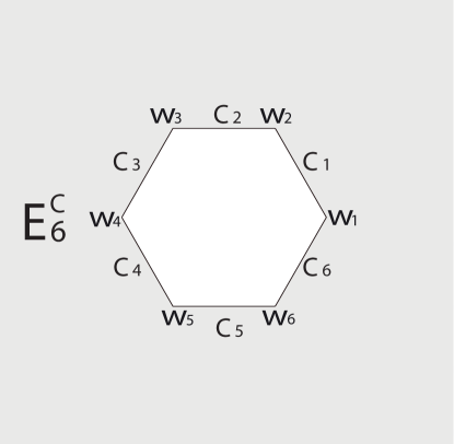
Figure 1: The normalized domain $E_{K}^{C}$, with $K=6$, as an illustrative example.

We can also write $\mathbf{P}$ in terms of an order parameter, $s$, and an angle $\gamma$ as shown below -

$$\mathbf{P}=2s\left(\mathbf{n}\otimes\mathbf{n}-\frac{1}{2}\mathbf{I}_{2}\right),$$ (4)

where $\mathbf{n}=\left(\cos\gamma,\sin\gamma\right)^{T}$ is the nematic director in the plane, and $\mathbf{I}_{2}$ is the $2\times 2$ identity matrix, so that

$$P_{11}=s\cos\left(2\gamma\right),\ P_{12}=s\sin\left(2\gamma\right).$$

The defect set is simply identified with the nodal set of $s$, also see han2020pol, interpreted as the set of no planar order in $E_{K}^{C}$.

We impose homeotropic boundary conditions on $\partial E_{K}$, which requires $\mathbf{n}$ in P to be homeotropic/normal to the edges of $E_{K}$. However, there is a necessary mismatch at the corners/vertices. We impose a continuous Dirichlet boundary condition, $\mathbf{P}=\mathbf{P}_{b}$, on $\partial E_{K}$ as defined below:

$$\aligned&P_{11b}\left(w\right)=\alpha_{k}=\cases{&}\frac{B}{2C}\left((1-\frac{a}{2})\cos\left(\frac{\left(2k-1\right)2\pi}{K}\right)+\frac{a}{2}\cos\left(\frac{\left(2k+1\right)2\pi}{K}\right)\right),||w-w_{k}||\geq||w-w_{k+1}||,\\ \frac{B}{2C}\left((1-\frac{a}{2})\cos\left(\frac{\left(2k-1\right)2\pi}{K}\right)+\frac{a}{2}\cos\left(\frac{\left(2k-3\right)2\pi}{K}\right)\right),||w-w_{k}||\leq||w-w_{k+1}||,\\ P_{12b}\left(w\right)=\beta_{k}=\cases{&}\frac{B}{2C}\left((1-\frac{a}{2})\sin\left(\frac{\left(2k-1\right)2\pi}{K}\right)+\frac{a}{2}\sin\left(\frac{\left(2k+1\right)2\pi}{K}\right)\right),||w-w_{k}||\geq||w-w_{k+1}||,\\ \frac{B}{2C}\left((1-\frac{a}{2})\sin\left(\frac{\left(2k-1\right)2\pi}{K}\right)+\frac{a}{2}\sin\left(\frac{\left(2k-3\right)2\pi}{K}\right)\right),||w-w_{k}||\leq||w-w_{k+1}||,$$ (5)

where $a(w,\sigma)\in[0,1]$, $w\in C_{k}$, $k=1,\cdots,K$ is an interpolation function, which is continuous and strictly monotonic about $||w-(w_{k}+w_{k+1})/2||$, increasing from $0$ at the centre of $C_{k}$, to $1$ at the two vertices of $C_{k}$. Further, we take $0<\sigma\leq 1/2$ and $a(w,\sigma)\to 0$ as $\sigma\to 0$. At the vertices $w=w_{k}$, we set $\mathbf{P}_{b}$ to be equal to the average of the two constant values on the two intersecting edges, and at the edge mid-point i.e., $w=(w_{k}+w_{k+1})/2$, we have strictly homeotropic conditions. As $\sigma\to 0$, the Dirichlet boundary conditions are piece-wise constant and compatible with strict homeotropic conditions P_11b(w) = ^α_k = B2Ccos((2k-1)2πK),   P_12b(w) = ^β_k = B2Csin((2k-1)2πK), w∈C_k.

Further, the domain $E_{K}^{C}$ is unbounded and we impose uniform/constant boundary conditions at infinity as given below:

$$\lim_{|w|\to\infty}\mathbf{P}=\mathbf{P}^{*}:=\frac{B}{C}(\mathbf{n}^{*}\otimes\mathbf{n}^{*}-\frac{1}{2}\mathbf{I}_{2}),$$ (6)

where $\mathbf{n}^{*}=(\cos(\gamma^{*}),\sin(\gamma^{*}))$ is the constant nematic director at infinity. To avoid confusion, we reiterate that $\gamma$ is the director angle and $\gamma^{*}$ is associated with the boundary condition at infinity.

The corresponding Euler-Lagrange equations are

$$\aligned\Delta P_{11}&=\frac{2C\bar{\lambda}^{2}}{L}\left(P_{11}^{2}+P_{12}^{2}-\frac{B^{2}}{4C^{2}}\right)P_{11},\\ \Delta P_{12}=\frac{2C\bar{\lambda}^{2}}{L}\left(P_{11}^{2}+P_{12}^{2}-\frac{B^{2}}{4C^{2}}\right)P_{12}.$$ (7)

For the purposes of this paper, the crucial dimensionless parameter is

$$\lambda^{2}=\frac{2C}{L}\bar{\lambda}^{2}$$

where the nematic correlation length, $\xi_{n}\propto\sqrt{\frac{L}{C}}$ at the fixed temperature $A=-\frac{B^{2}}{3C}$. Recall that $L$ has units of Newton (N) and $C$ has units of $Nm^{-2}$, so that $\xi_{n}$ has the units of length.

The admissible space is &H_∞:=P^* + H,
H:={H∈H^1_loc(E_K^C;S_0):∫_E_K^C—∇H—^2 + ∫_E_K^C—H—2—w—2¡∞} where

$$\mathcal{S}_{0}:=\{\mathbf{P}\in M_{2}(\mathbb{R}):P_{ij}=P_{ji},tr(\mathbf{P})=0\}.$$

The free energy p_energy is not always finite, since the potential term $f_{b}\geq 0$ may very well not be integrable in $E_{K}^{C}$. However, since $f_{b}(\mathbf{P}^{*})=0$, we may find a compactly supported $\mathbf{H}\in\mathcal{H}$, for which $\mathbf{P}=\mathbf{P}^{*}+\mathbf{H}$ satisfies the boundary condition Pb. The existence of solution of Euler_Lagrange in $\mathcal{H}_{\infty}$, has been proven in Proposition 3 of Bronsard2016minimizers.

We study two distinguished limits in what follows—the $\lambda\to 0$ limit which is relevant for polygon holes $E_{K}$ with edge length comparable to $\xi_{n}$ which is typically on the nanometre scale, and the $\lambda\to\infty$ limit, which is the macroscopic limit relevant for micron-scale or larger polygonal holes. In the following sections, we study the limiting problems and the limiting minimiser profiles, their defect sets and multistability in the $\lambda\to\infty$ limit.

III The $\lambda\to 0$ limit

In Theorem 1 of Bronsard2016minimizers, as $\lambda\to 0$, the solution of Euler_Lagrange converges to the unique solution of zero_euler below, with Dirichlet boundary conditions.

$$\aligned&\Delta P_{11}^{0}=0,\ \Delta P_{12}^{0}=0,on\ E_{K}^{C},\\ P_{11}^{0}=P_{11b},\ P_{12}^{0}=P_{12b},\ on\ \partial E_{K},\\ \mathbf{P}=\mathbf{P}^{*},\ |x|\to\infty.$$ (8)

In other words, the limiting problem is a boundary-value problem for the Laplace equation for $\mathbf{P}$ on $E^{C}_{K}$, in the $\lambda\to 0$ limit. This problem is explicitly solvable and in the following sections, we exploit the symmetries of the Laplace equation, the symmetries of the polygon and boundary conditions to illustrate how the limiting profile depends on $K$ - the number of polygon edges, and $\gamma^{*}$ - the director angle at infinity. In fact, these two parameters tune the existence, location and dimensionality of defects in this limit, amenable to experimental verification in due course.

III.1 Defect patterns outside a 2D disc

As an illustrative example, we first consider the limiting problem zero_euler on the complement of a disc. As $K\to\infty$, the domain, $E_{K}^{C}$, converges to the exterior of a disc, $D^{C}$. The conformal mapping from unit disc, $D$, to exterior of disc, $D^{C}$, is given by

$$w=f(z)=\frac{1}{z}.$$

Under the mapping $f^{-1}:D^{C}\to D$, the limiting problem for $\lambda=0$ is given by: &Δp_11 = 0,  Δp_12 = 0, z∈D
p_11 = B2Ccos(-2θ), p_12 = B2Csin(-2θ), z∈∂D
p_11 = B2Ccos(2γ^*), p_12 = B2Csin(2γ^*), z=0 where $z=re^{i\theta}$, $\theta$ is the azimuthal angle and $r$ is the radius. The corresponding solution is p_11(re^iθ,γ^*) &= B2C(r^2cos(-2θ) + lim_ϵ→0cos(2γ*)ln rln ϵ),
p_12(re^iθ,γ^*) = B2C(r^2sin(-2θ) + lim_ϵ→0sin(2γ*)ln rln ϵ). This solution has the rotational symmetry property (p_11,p_12)(re^iθ,γ^*) = (p_11(re^iθ+iγ^*,0)cos2γ^* - p_12(re^iθ+iγ^*,0)sin2γ^*,
p_12(re^iθ+iγ^*,0)cos2γ^* + p_11(re^iθ+iγ^*,0)sin2γ^*), so that it suffices to assume $\gamma^{*}=0$. With $\gamma^{*}=0$, we can check that $p_{11}=p_{12}=0$ at exactly two points, located at $\theta=\frac{\pi}{2}$ and $\theta=\frac{3\pi}{2}$ respectively. The corresponding limiting solution on $D^{C}$ is:

$$\mathbf{P}(w,\gamma^{*})=\mathbf{p}(f^{-1}(w),\gamma^{*})=s_{+}\left(\frac{1}{\rho^{2}}(\mathbf{e}_{\rho}\otimes\mathbf{e}_{\rho}-\mathbf{I}_{2}/2)+\lim_{\epsilon\to 0}\frac{ln\rho}{ln1/\epsilon}(\mathbf{n}^{*}\otimes\mathbf{n}^{*}-\mathbf{I}_{2}/2)\right)$$ (9)

where $w=\rho e^{i\psi}$,$\mathbf{e}_{\rho}=(\cos\psi,\sin\psi)$ is the unit radial vector and the constraint at infinity is $\mathbf{n}^{*}=\left(\cos\gamma^{*},\sin\gamma^{*}\right)$.

This method can be easily generalised to piecewise constant boundary conditions on segments of $\partial D$, relevant for solving the limiting problem (8) on $E^{C}_{K}$, as we shall see in the Section 3.3. Consider the following boundary-value problem on the unit disc $D$, &Δu = 0, z∈D,
u = u_k, on z∈D_k, k = 1,⋯, K,
u = u_0, on z = 0. where

$$D_{k}=\{e^{i\theta},\theta\in(-2\pi k/K,-2\pi k/K+2\pi/K)\},\ k=1,...,K,$$ (10)

are the segments of $\partial D$. The solution, $u$, can be written as, $u=u_{a}+u_{b}$, where $u_{a}$ and $u_{b}$ are defined by the following boundary-value problems: &Δu_a = 0, z∈D,
u_a = u_k, on z∈D_k, k = 1,⋯, K,
u_a = 12π∑_k = 1^K ∫_2π(K-k)/K^2π(K-k+1)/Ku_k dϕ  on  z=0, and &Δu_b = 0, z∈D,
u_b = 0, on z∈D_k, k = 1,⋯, K,
u_b = u