Abstract
Low frequency radio observations of galaxy clusters are a useful probe of the non-thermal intracluster medium (ICM), through observations of diffuse radio emission such as radio halos and relics. Current formation theories cannot fully account for some of the observed properties of this emission. In this study, we focus on the development of interferometric techniques for extracting extended, faint diffuse emissions in the presence of bright, compact sources in wide-field and broadband continuum imaging data. We aim to apply these techniques to the study of radio halos, relics and radio mini-halos using a uniformly selected and complete sample of galaxy clusters selected via the Sunyaev-Zel’dovich (SZ) effect by the Atacama Cosmology Telescope (ACT) project, and its polarimetric extension (ACTPol). We use the upgraded Giant Metrewave Radio Telescope (uGMRT) for targeted radio observations of a sample of 40 clusters. We present an overview of our sample, confirm the detection of a radio halo in ACTCL J0034.4+0225, and compare the narrowband and wideband analysis results for this cluster. Due to the complexity of the ACTCL J0034.4+0225 field, we use three pipelines to process the wideband data. We conclude that the experimental spam wideband pipeline produces the best results for this particular field. However, due to the severe artefacts in the field, further analysis is required to improve the image quality.
keywords:
galaxies; clusters; individual–galaxies; clusters; intracluster medium–radio continuum1 \issuenum1 \articlenumber0 \externaleditorAcademic Editor: Francesca Loi \datereceived \dateaccepted \datepublished \hreflinkhttps://doi.org/ \TitleA GMRT Narrowband vs. Wideband Analysis of the ACTCL J0034.4+0225 Field Selected from the ACTPol Cluster Sample \TitleCitationA GMRT Narrowband vs. Wideband Analysis of the ACTCL J0034.4+0225 Field Selected from the ACTPol Cluster Sample \AuthorSinenhlanhla P. Sikhosana 1,2,*\orcidA, Kenda Knowles 3,4\orcidB, C.H. Ishwara-Chandra 5\orcidF, Matt Hilton 1,2\orcidC, Kavilan Moodley 1,2\orcidD and Neeraj Gupta 6\orcidE \AuthorNamesSinenhlanhla P. Sikhosana, Kenda Knowles, C. H. Ishwara-Chandra, Matt Hilton, Kavilan Moodley and Neeraj Guptae \AuthorCitationSikhosana, S.P.; Knowles, K.; Ishwara-Chandra, C.H.; Hilton, M.; Moodley, K.; Guptae, N. \corresCorrespondence: SikhosanaS@ukzn.ac.za
1 Introduction
Non-thermal diffuse emission in galaxy clusters was first discovered in the Coma cluster (Large et al., 1959; Brown and Rudnick, 2011; Bonafede et al., 2020). This discovery was a confirmation of the existence of relativistic electrons and magnetic fields in the intracluster medium (ICM) Sarazin (1988); Kravtsov and Borgani (2012). Traditionally, diffuse radio emissions have been categorized into three groups based on morphology, size, and cluster dynamics; giant radio halos (GRHs), radio mini-halos (RMHs), and radio relics (RRs). The size of these non-thermal diffuse structures, which extend over kpc to Mpc scales, raised questions on their formation mechanisms. One prominent question is how the cosmic ray electrons (CRes) are (re)accelerated and transported given their diffusion timescale limitations Enßlin et al. (2011). Many studies have been conducted to formulate and constrain theories detailing the formation of these sources.
GRHs, Mpc-scale sources with low polarization percentages (<10) located in the central regions of clusters, have two main formation theories. The first is the secondary ‘hadronic’ model, in which electrons originate from hadronic collisions between the long-living relativistic protons in the ICM and thermal ions Dennison (1980); Pfrommer et al. (2008); Enßlin et al. (2011). This formation theory has not been widely accepted due to the lack of observational evidence of gamma rays in clusters, which are a by-product of the hadronic processes Reimer et al. (2003); Ackermann et al. (2010, 2018). Although observations disfavour the hadronic model as the primary source of radio halo emission, hybrid models suggest that these hadronic interactions may produce a seed population of electrons that is then re-accelerated to form GRHs (Brunetti and Blasi, 2005; Brunetti et al., 2017).
The second model is the primary ‘re-acceleration’ model. According to this model, a pool of pre-existing electrons Pinzke et al. (2017) is re-accelerated through second order Fermi mechanisms by ICM turbulence developing during cluster mergers Brunetti et al. (2001); Feretti et al. (2012); Donnert and Brunetti (2014). A strong dynamical link has been found with respect to the host clusters Markevitch et al. (2005); Lindner et al. (2014); Kale et al. (2015). The Mpc-scale emission has mostly been found in massive (M500,SZ > 4 M⊙) clusters with X-ray and optical merger signatures Cassano et al. (2013). The power of the radio emission has been found to correlate with thermal host cluster properties, with non-detections lying below the correlation and with sources that exhibit ultra-steep spectra (\endnoteS 1.5) that populate the region between the correlation and upper limits, as predicted by the re-acceleration model Brunetti and Jones (2014). Studies have shown that cluster selection methods affect the resulting scaling relations. Samples selected via their Sunyaev-Zel’dovich signal (SZ; Sunyaev and Zeldovich (1972)) show a higher detection rate than X-ray-selected samples Cuciti et al. (2015, 2021). This difference may be due to the different time-scales of boosting the SZ vs X-ray emission during mergers. Although the re-acceleration theory is widely accepted, there are still a few aspects that need further investigation. A major open question is the origin of the re-accelerated cosmic ray particles (Brunetti and Jones, 2014; van Weeren et al., 2019).
RMHs are similar in morphology to GRH; however, they extended over a few 100 kpc in scale and are generally found in non-merging cool-core clusters. These sources are located around the brightest cluster galaxies (BCGs). RMHs form as a result of re-acceleration of seed electrons by the turbulence induced from gas sloshing in the cool core Gitti et al. (2002). Brunetti and Jones (2014) suggest that there is an intermediate transition stage where GRHs transition to RMHs or vice-versa. This has been the explanation used for the existence of GRHs in cool-core clusters Bonafede et al. (2014); Parekh et al. (2021).
RRs are arc-shaped, Mpc scale, highly polarised sources (20) that are located at the peripheral region of the clusters. Several observations have shown that their origin is linked to shock waves generated in the ICM by merger events Jaffe and Rudnick (1979); Enßlin et al. (1998); Bonafede et al. (2012); Botteon et al. (2016); Locatelli et al. (2020). However, the underlying particle acceleration mechanism is still under debate Stuardi et al. (2019). In the mechanism of first-order diffusive shock acceleration (DSA; Bell (1978); Jones and Ellison (1991)), cosmic-ray protons and electrons are assumed to be accelerated from the thermal pool up to relativistic energies at the cluster merger shocks. Although this mechanism can explain the general properties of relic emission, several observational features remain unexplained Stuardi et al. (2019), such as the non-detection of gamma rays in clusters that host RRs Ackermann et al. (2018) and the low Mach numbers observed in shocks Brunetti and Jones (2014).
The second mechanism proposes the re-acceleration of fossil relativistic electrons via DSA at the cluster shocks Markevitch et al. (2005); Pinzke et al. (2013); Kang et al. (2017). This mechanism reproduces the observed spectrum de Gasperin et al. (2014); Shimwell et al. (2015); van Weeren et al. (2017) and does not require shocks to have large Mach numbers, as the pre-existing electrons have enough energy to be re-accelerated to relativistic speeds Brunetti and Jones (2014). However, this mechanism also presents challenges as there are expected phenomena that are yet to be observed Stuardi et al. (2019). For example, the connection between active galactic nuclei (AGN; candidate seed electron source) and radio relics could be established only in a few cases Bonafede et al. (2014); van Weeren et al. (2017). A model by Zimbardo and Perri (2017, 2018) focuses on the role of magnetic fields that under specific configurations could allow electrons to reach relativistic speeds via the shock drift acceleration mechanism (SDA; Guo et al. (2014); Caprioli and Spitkovsky (2014)). However, the role of magnetic fields and its amplification by low Mach number shocks is still poorly constrained Stuardi et al. (2019).
A new generation of telescopes such as the LOw-Frequency ARray (LOFAR; van Haarlem et al. (2013)), MeerKAT Jonas and MeerKAT Team (2016), and the uGMRT (Gupta et al., 2017) have opened a window into a new group of ultra-steep radio sources which were previously undetectable due to frequency and sensitivity constraints. The new studies have resulted in a different class of diffuse emission, such as; radio phoenices and gently re-energized tails (GReETs; de Gasperin et al. (2017); van Weeren et al. (2019)). The sensitivity of these telescopes have opened up a new observational window which probes lower mass (4 1014 M⊙) and higher redshift ( 0.3) clusters (Knowles et al., 2019; Giovannini et al., 2020; Raja et al., 2021). Large cluster samples of this nature will help in the refinement of currently existing formation theories. However, the broad bandwidths and large fields of view of these telescopes also present multiple data reduction challenges.
In this paper, we introduce an SZ-selected sample from the ACTPol observations. We will also discuss the challenges we faced with the uGMRT data reduction and present a case study of ACTCL J0034.4+0225 (hereafter J0034). In Section 2, we introduce the cluster sample. In Section 3, we discuss the data reduction challenges and the pipelines we explored. In Section 4, we study J0034 and compare the narrowband and wideband results. Finally, we summarise our findings and future outlook in Section 5. We adopt a CDM flat cosmology with = 70 km s-1 Mpc-1, = 0.3, and = 0.7. For our radio spectral index calculations, we assume S, where is the flux density at frequency and is the spectral index.
2 The ACTPol Sample
Until recently, statistical studies of diffuse radio emission in galaxy clusters have been constrained to observations of high mass and low redshift systems selected using X-ray telescopes Venturi et al. (2008); Kale et al. (2015). The X-ray selected samples had relatively low diffuse emission detection rates (20). Andrade-Santos et al. Andrade-Santos et al. (2017) studied the fraction of cool-core clusters in an X-ray selected sample from Chandra versus an SZ selected sample from Planck. Their study revealed that the X-ray sample had a higher fraction (44) of cool-core clusters in comparison to the SZ sample (28). The majority of cool-core clusters do not host GRHs and RRs; and hence would attribute to the low detection rates. These findings in conjunction with the poor resolution (1.8′) of ROSAT, which was mainly used for the X-ray samples, may account for the low detection rates of diffuse emission in X-ray selected samples. Such constraints have since led to preferentially using SZ-selected samples for scaling relation studies.
The thermal SZ effect is a powerful probe for high-redshift clusters due to the fact that it is not affected by dimming. Hence, the SZ survey catalogues offer an almost redshift independent selection function. Essentially, cluster samples from SZ surveys are restricted by cluster masses based on the sensitivity of the observing instrument. The three main microwave telescopes that have been used to detect galaxy clusters are the ACT, the Planck satellite Planck Collaboration et al. (2011), and the South Pole Telescope (SPT; Carlstrom et al. (2011)).
For our project, we use the galaxy cluster catalogue from the ACT’s Polarimetric extension (ACTPol; Louis et al. (2017)) to select our sample. The ACTPol catalogue was constructed using the ED56 region, shown in Figure 1, which covers an area of 987.5 deg2 Hilton et al. (2018).
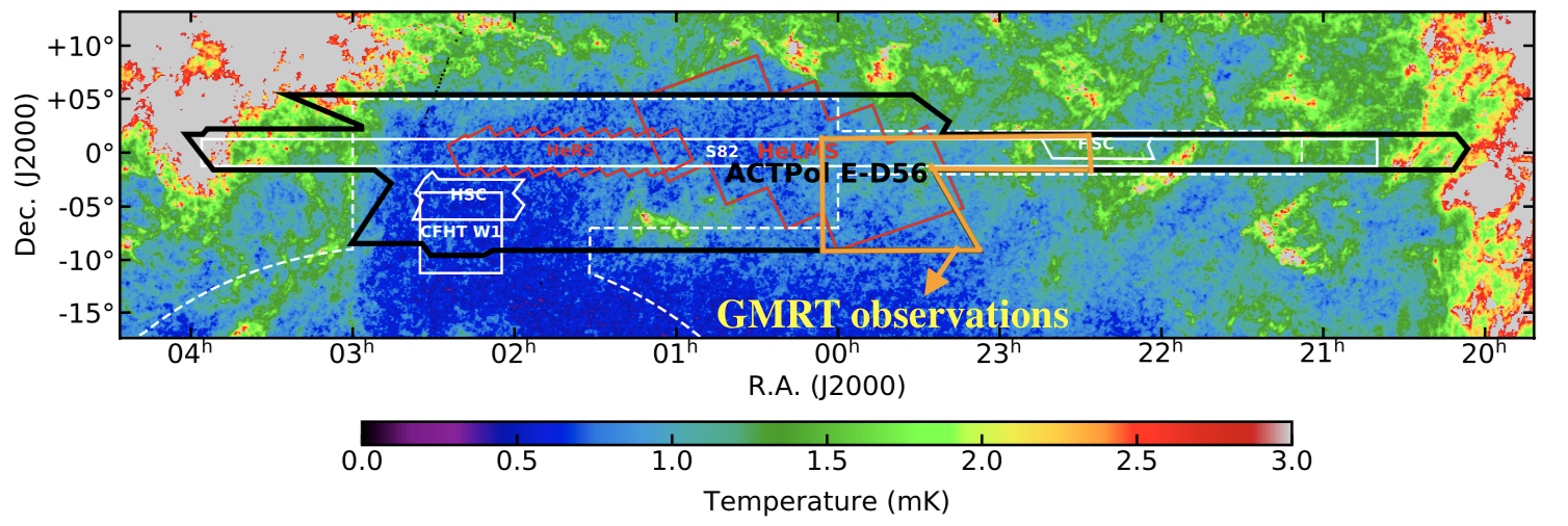
2 \switchcolumnThe final catalogue consists of 182 optically confirmed clusters. For a signal-to-noise (SNR) 4 the sample spans a mass and redshift range of 1.6 1014 M⊙ 9.1, and 0.1 1.4, respectively. The 90 sample completeness cut-off is for SNR 5 and a redshift range of 0.2 1.0. M500c is the mass measured within a radius that encloses a region with an average density that is 500 times the critical density at the cluster redshift, and assuming the SZ-signal scales with mass as described in Arnaud et al. Arnaud et al. (2010).
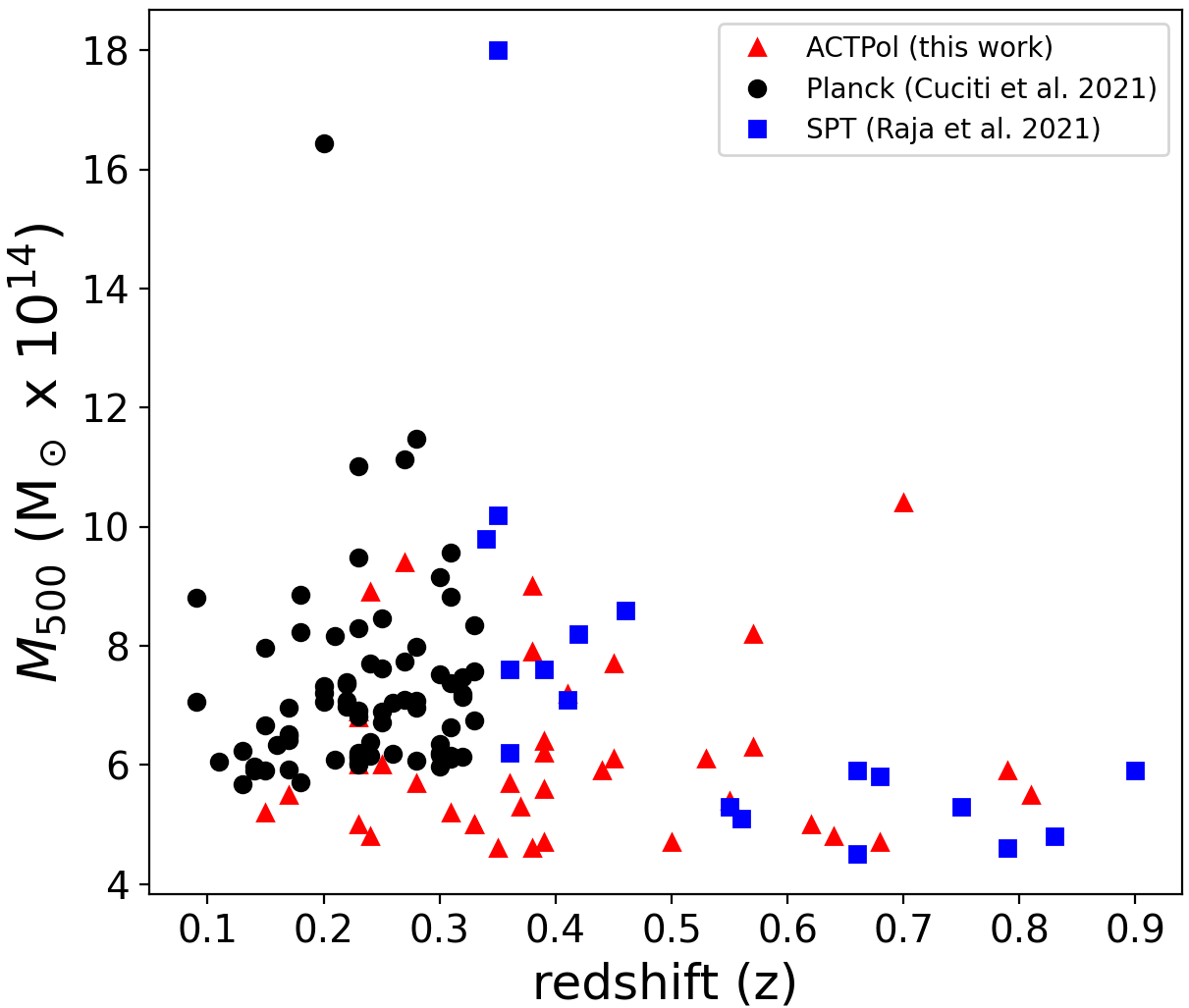
For our sample, we considered all the clusters with an SNR 5. We then applied a mass and redshift cut of M500,SZ 4 1014 M⊙ and 0.1 0.8. This results in a sample of 40 clusters, which formed the basis of our sample. Given that the ACTPol catalogue is 90 complete for clusters within 0.2 1.0 and , we derive our sample completeness to be 68. This completeness is derived from the mass completeness and the available radio information (30/40). In Figure 2, we compare our sample of 40 clusters to Planck and SPT samples, which are the most recent statistical studies using SZ-selected cluster samples. Our sample covers a wider redshift range compared to both samples. We also cover lower mass clusters compared to the Planck sample. The SPT sample overlaps with ours at higher redshifts; however, it does not cover lower redshifts ( 0.33). This study is a precursor to studies of larger samples exploring lower mass and higher redshift cluster sample studies such as the MeerKAT Extended Relics, Giant Halos, and Extragalactic Radio Sources (MERGHERS) survey Knowles et al. (2016) and the MeerKAT Absorption Line Survey (MALS; Gupta et al. (2016)).
We chose to observe these clusters at low-frequency (250–500 MHz) using the wideband uGMRT in addition to using existing archival narrowband GMRT data. As of November 2020, there were 17 clusters with pre-existing GMRT legacy software backend (GSB) observations. The GSB has a bandwidth of 32 MHz. We obtained uGMRT wideband (GWB) observations for 13 clusters, taken over three observing semesters. These clusters were observed in GMRT’s observing cycles 32, 33, and 36 (proposal IDs: 32012, 33010, 36050). In total, we have 30 clusters with narrowband and/or wideband observations. For this paper, we focus on the data reduction and analysis of J0034, which has both narrowband and wideband observations. We selected this field because it was most severely affected by RFI and has multiple bright sources near the cluster region. Hence, successfully calibrating and imaging this field would imply that we could apply the techniques on the rest of the sample.
3 Data Reduction
For this paper, we focus on the case study of the complex field J0034. We start by reducing the narrowband observations using the source peeling and atmospheric modelling (SPAM; Intema (2014); Intema et al. (2017)). The final narrowband image indicates that this field has bright sources near the cluster’s region. Such sources complicate the calibration procedure. Such a field is a good case study for testing calibration and imaging strategies. Hence, when reducing the wideband data, we use three pipelines and compare the resulting images for J0034. In the following sections, we discuss the narrowband and wideband data reduction strategies.
3.1 Legacy GMRT GSB
We use spam’s calibration pipeline version 19.11.07 to reduce the GSB data. spam is a fully automated Python pipeline that uses the parseltongue Kettenis et al. (2006) interface to access and execute the Astronomical Image Processing System (AIPS; van Moorsel et al. (1996)) tasks. The pipeline is divided into two steps; the ‘pre-calibrate targets’ step and the ‘process target’ step. The data reduction steps are as follows.
-
1.
The ‘pre-calibrate target’ step performs the cross-calibration step of the standard calibration procedure. The pipeline uses the primary calibrator(s) to determine the channels affected by RFI, determine the flux scale, and to produce cross calibration tables. The flags and calibration tables are then applied to the target source. Finally, the calibrator and target visibilities are split into separate UVFITS files.
-
2.
The ‘process target’ step begins by taking the cross-calibrated (1GC) target data and applying 2GC (or self calibration). For 2GC, the target visibilities are imaged using the facet-based method established by Cornwell and Perley (1992). The point sources covering the primary beam are obtained from a sky model extracted from the VLA low-frequency sky survey (VLSS; (Cohen et al., 2007)) and the NRAO VLA sky survey (NVSS; (Condon et al., 1998)). The observed field is then faceted based on the sky model. The deconvolution is done using the Cotton-Schwab clean algorithm (Condon et al., 1998). The cleaned visibilities are calibrated using the sky model. Then the calibrated visibilities are imaged to produce a better sky model and improved calibration solutions. This self calibration cycle is applied three times. For the wide-field imaging, the pipeline performs a single-scale CLEAN deconvolution down to 3 times the central background noise (), using automated CLEAN boxes placed at positive peaks of at least 5.
-
3.
The second part of the ‘process target’ step is to correct for DDEs (3GC), which include ionospheric effects (Lonsdale, 2005). For each 3GC cycle, the brightest source in the field is peeled. The ionospheric effects of the brightest source are modelled and phase corrected solutions for the peeled model are obtained. spam uses a phase screen model to extend the ionospheric phase solutions of the single source to the full field. Then the solutions are applied to each facet during imaging. This cycle is repeated six times, and each time the brightest source is selected and corrected for DDEs. This repeats until all the bright sources are corrected for DDEs. Finally, the astrometric corrections are applied to the DDEs corrected image and the image is primary beam corrected thereafter.
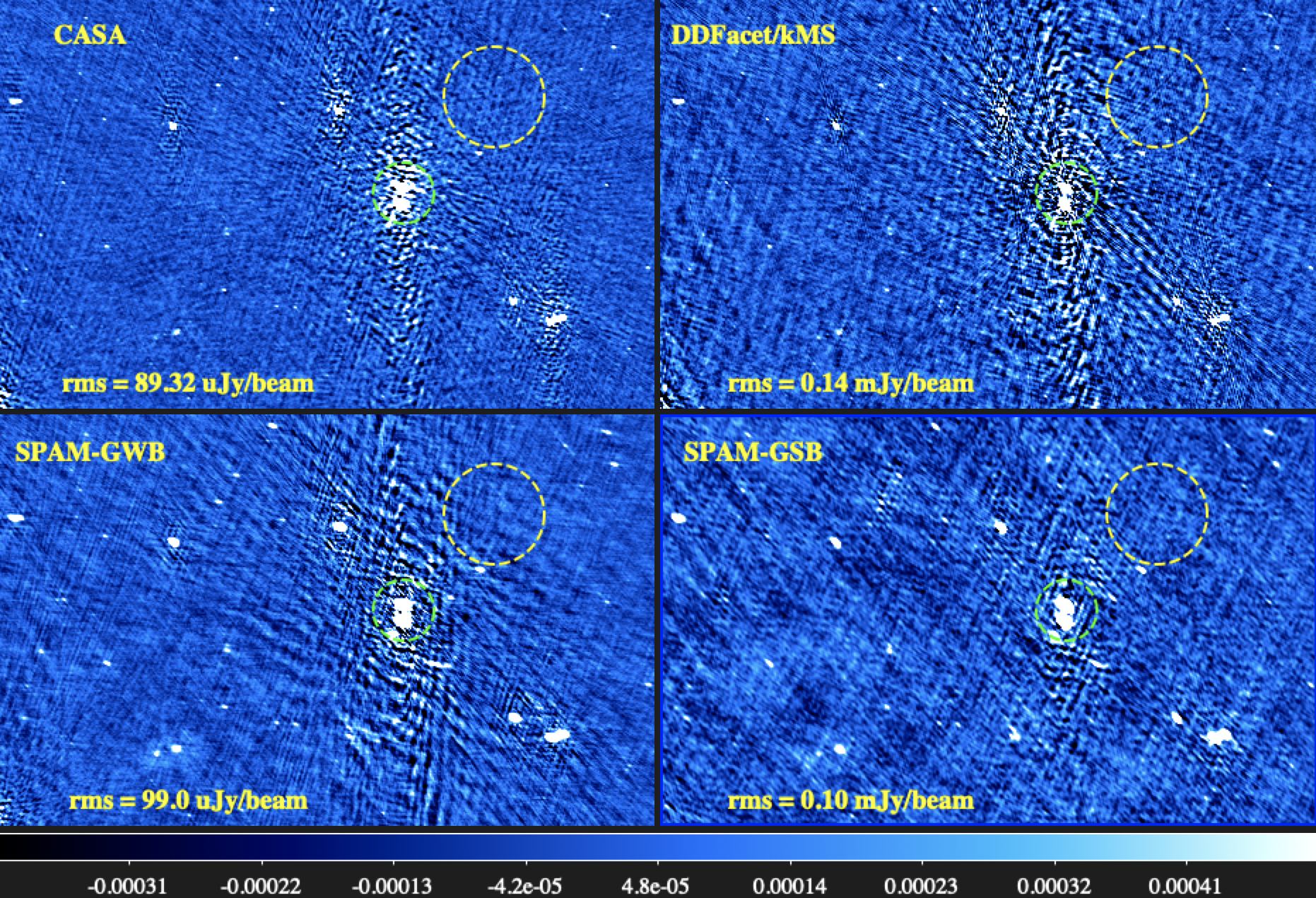
We used default data reduction parameters throughout the different stages of the pipeline. The default setting of the number of pixels is 3780, with a pixel size of 1.9′′ and the robust parameter is 1. The resulting image, shown in the bottom right panel of Figure 3, has a rms of 0.10 mJy/beam near the cluster centre, and the beam size is 18.1′′ 14.2′′, p.a. 60.3∘.
3.2 uGMRT Data Reduction
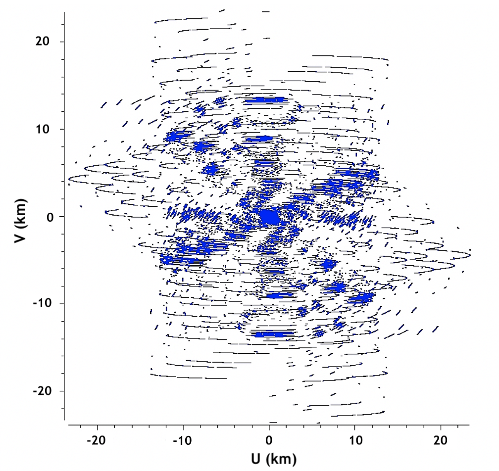
Thirteen clusters in our sample, including J0034, have uGMRT GWB band 3 (250–500 MHz) observations. The wide bandwidth of the upgraded GMRT simultaneously provides increased sensitivity and opportunity for in-band spectral index studies. However, the calibration and imaging of GWB data is a complex procedure. The main challenges with reducing the wideband, wide-field data are as follows. The primary beam pattern is dependent on the observing frequency, hence, for wide bandwidth observations, this pattern varies across the band. The flux density of radio sources correlates with the frequency (S). As a result of this correlation, the spectral models of the point sources need to be taken into account during imaging. The uGMRT observations were carried out at low-frequencies, which resulted in various directional dependent effects, such as ionospheric effects. The GWB observations of J0034 are particularly affected by radio frequency interference (RFI), which corrupts data if not fully modelled and removed. The level of RFI in our data makes the reduction process onerous and leads to images with significantly compromised quality. The resulting images had rms noise values three to seven times higher than the theoretically predicted noise floor of 10 Jy/beam. Another challenge for our sample was that it is in the equatorial region (7.2∘ 4∘), so despite the wide bandwidth and hours of integration time, coverage is more sparse because aperture synthesis is not as effective for equatorial sources (see Figure 4). The poor sampling of the visibility space results in north-south artefacts around bright sources, which are a reflection of the poor sampling function.
To overcome these challenges, we explored various pipelines that deal with the intensive RFI flagging and calibration direction-dependent effects. Once the data reduction pipelines are refined, we plan to reduce the remaining wideband data to determine if we can detect lower surface brightness diffuse emission in clusters with non-detections in the GSB data, and enhanced features of the existing diffuse emission detections in other clusters. The pipelines we explored are summarised below, including the image comparison of the J0034 results.
3.2.1 CASA Pipeline
The casa pipeline we adopt is a preliminary version of the capture pipeline Kale and Ishwara-Chandra (2020). For this pipeline, flagging, calibration and imaging is done using in-built Common Astronomy Software Applications (casa; McMullin et al. (2007)) tasks. Firstly, we flag RFI using the manual and automated flagdata tasks. We apply the auto-flag separately for the different fields. For auto-flagging, we use the tfcrop mode which identifies and removes outliers on the time-frequency plane. We set the flagging threshold parameters higher for the calibrator fields in comparison to the target field because these fields are usually much brighter and are detected at a higher SNR. The timecutoff and freqcutoff deviation parameters for the calibrators were set to 5.0, while for the target they were set to 6.0. These values place constraints on the deviation of data points from the fitted time and frequency polynomial. Data points with higher deviation values are regarded as RFI.
We then apply a cycle of cross-calibration. We begin by setting the flux scale using the standard models from Perley and Butler (2013). Thereafter, we produce calibration tables. The delay calibration solution interval is 10 min, and we only have one solution interval for bandpass and gain calibration. We transfer the flux and phase calibration solutions to the target. After the first cycle of cross-calibration, we apply flagging once more. We do this in order to excise low-level RFI only discernible after calibration. This time we use tfcrop and rflag mode. The rflag mode calculates statistics per time chunk and set thresholds which indicate the outliers that need to be flagged. We apply rflag post calibration because it tends to result in higher flag percentages if applied on uncalibrated data. Finally, we produce calibration solutions from the second cycle of cross-calibration and apply these solutions to the target.
We then separate the target visibilities and begin with 2GC. We apply multiple cycles of phase-only calibration on the data, we stop once the quality of the image is no longer improving. For most data sets, the four cycles were sufficient. We then apply multiple cycles of phase and amplitude calibration until the noise quality of the images reaches a plateau, three cycles were sufficient for most datasets. For both phase-only and phase and amplitude calibration, we begin with a solution interval of 16 min and decrease the interval per cycle by dividing the initial solution interval by a factor of two times the number of the cycle. Our imaging during self-calibration is done using tclean’s mtmfs deconvolver, with nterms = 2 and robust parameter = 0. This deconvolver accounts for the varying spectral indices of sources across the wide bandwidth. The number of iterations is set to 2500 and increases per cycle by a factor of 2n, where n is the cycle number. The mask is set to auto-multithreshold. The CLEANing threshold is 0.01 mJy while the sidelobe threshold is set to 3.
The resulting image, shown in the top left panel of Figure 3, has a rms of 89.2 J/beam and the beam size is 8.0′′ 4.9′′, p.a. 60.3∘. The GSB image is included in the panels for comparison purposes. After rigorous RFI excision strategies, including aoflagger Offringa et al. (2012), the north–south artefacts around the bright sources were still visible. This led us to conclude that these artefacts and phase variations in the bright sources are due to DDEs. The results of this pipeline were unsatisfactory for our science goals, since we needed to correctly remove bright point sources in the visibilities. Hence, we explored other pipelines which apply DDEs calibration (3GC).
3.2.2 DDFacet/killMS Pipeline
The killms\endnotehttps://github.com/saopicc/killMS (the pipeline was accessed in August 2019) and ddfacet (Tasse et al., 2018) based pipeline attempts to correct for DDEs by solving the full Jones matrix. This pipeline starts with a measurement set (MS) that has been calibrated using the casa pipeline. From our investigation of the casa pipeline, we found that more cycles of 2GC calibration resulted in images with lower peak fluxes. Hence, for this pipeline, 2GC is only applied once for phase-only calibration. We use the image produced after 2GC to create a mask using a threshold of 10 to ensure we create a sky model that does not contain residual artefacts. Thereafter, we image the visibilities using ddfacet. The imaging parameters used are as follows. We apply three major cycles and 90,000 minor cycles with a deconvolution peak factor of 0.001. These parameters are fixed even for the post-killms imaging cycle.
We then examine the 2GC image and locate the brightest sources (0.1 Jy) in ds9 Joye and Mandel (2003), and create a bright-source region file. A minimum of three sources is tagged for each field, and a maximum of 6 sources are tagged for fields with numerous bright sources. We use the region file to divide the target field into facets equal to the number of bright sources in the region file, with the tagged sources being at the phase centre of each facet. We use killms to obtain a set of direction-independent solutions for each facet separately, which is combined into a set of direct-dependent solutions for the field. We apply the CohJones solver with a time solution interval of 5 min and frequency interval of 8 channels per solution. The number of directions we solve for is equivalent to the number of the bright sources that are tagged per field. Finally, we use ddfacet to apply the killms solutions and produce the DDEs corrected image. ddfacet also applies direction-dependent PSF deconvolution, which explicitly accounts for the time variation and bandwidth fluctuation effects. We perform the killms and ddfacet loops iteratively, improving the mask and increasing the time solution intervals with each loop until we get an image with significantly reduced artefacts.
The resulting image, shown in the top right panel of Figure 3, has a rms of 0.14 mJy/beam and the beam size is 7.9′′ 4.5′′, p.a. 52.4∘. We note that the noise floor is higher than thecasa result. The noise for the J0034 field increases by 4. However, the sources in this pipeline have a better defined structure compared to casa. The point sources are circular and have less phase variation. This indicated that the pipeline improved the phase corrections for the fields. Although the phase corrections had improved in comparison to the casa pipeline, the north–south artefacts were still not significantly reduced. Such artefacts would have been problematic for the point source subtraction, which is often required when extracting measurements for faint extended emission. We tried various calibration solution intervals (30 s–2 min) and facet numbers (3–8); however, these did not improve our results. The range of calibration solution intervals produced the same results, while increasing the facet numbers resulted in some facets having higher noise levels due to fewer sources in each facet.
3.2.3 Experimental SPAM Wideband Pipeline
The final pipeline we explored was the experimental wideband spam\endnotehttp://www.intema.nl/doku.php?id=huibintemaspampipeline (the pipeline was accessed in October 2020). This pipeline begins by splitting the GWB data into 7 sub-bands of 30 MHz each. Thereafter, it follows the conventional GSB narrowband data reduction for the individual sub-bands (see Section 3). The calibrated sub-band visibilities are then converted into MS files and concurrently imaged using wsclean. For the wsclean wide bandwidth imaging step, we use a Briggs robust = 0, number of iterations = 150,000, threshold = 1 Jy, auto-mask = 9, amd multiscale scales of (10,20,30).
The resulting image, shown in the bottom left panel of Figure 3, has a rms of 99.0 J/beam and the beam size is 14.0′′ 7.6′′, p.a. 65.3∘. As seen in the bottom left panel of Figure 3, this pipeline produces the best phase calibration, which results in an improvement in the structure of the brightest sources. The flag percentages in Table 3.2.3 also show that the spam pipeline results in the least flag percentages. These low percentages result in higher sensitivity, and this is indicated by the higher peak flux recovered for the double-lobed source shown in Figure 3.
[H] \tablesize \widetableJ0034 GWB data reduction pipelines’ image comparison. Columns: (1) Name of pipeline. (2) Effective observing frequency. (3) Synthesised beam of the image. (4) Flagged data. (5) Overall rms of the full resolution images. (6) Peak brightness of the double lobed source. \PreserveBackslash Pipeline \PreserveBackslash \PreserveBackslash Flags \PreserveBackslash Synthesised Beam \PreserveBackslash RMS \PreserveBackslash Peak Brightness \PreserveBackslash \PreserveBackslash MHz \PreserveBackslash \PreserveBackslash ′′ ′′, PA() \PreserveBackslash Jy/beam \PreserveBackslash Jy/beam \PreserveBackslash casa \PreserveBackslash 397 \PreserveBackslash 46.8 \PreserveBackslash 8.0 4.9, 60.3 \PreserveBackslash 38.9 \PreserveBackslash 0.13 \PreserveBackslash ddfacet/killms \PreserveBackslash 397 \PreserveBackslash 35.6 \PreserveBackslash 7.9 4.5, 52.4 \PreserveBackslash 40.5 \PreserveBackslash 0.19 \PreserveBackslash spam GWB \PreserveBackslash 398 \PreserveBackslash 24.4 \PreserveBackslash 14.0 7.6, 65.3 \PreserveBackslash 45.9 \PreserveBackslash 0.27 \PreserveBackslash spam GSB \PreserveBackslash 323 \PreserveBackslash 14.7 \PreserveBackslash 18.1 14.2, 48.2 \PreserveBackslash 75.8 \PreserveBackslash 0.34 {paracol}2 \switchcolumn
Although the noise levels are higher compared to the casa pipeline for both images, the improvement of the phase calibrations meant we would be able to extract the bright point sources, which is a necessary step when extracting faint diffuse emission. The peak fluxes of the sources in the spam-reduced images were much higher in than those in the casa-reduced and ddfacet/killms-reduced images. This indicates that the phase and amplitude calibration is improved, despite the higher noise floor, so that less of the real signal is being fractured into artefacts or side lobes. However, further steps are needed to improve the algorithm so that the 3GC strategy is more robust. These steps include more comprehensive ionospheric corrections in the sub-band data reduction and primary beam correction for the full bandwidth image.
3.3 Flux Density and P1.4GHz Calculations
We use the 2GC calibrated data to search for extended diffuse radio emission in the cluster region. To enhance the brightness of the diffuse emission, we produce a low resolution image. For the low resolution imaging process, we use the spam pipeline. We first image the compact sources by applying a -range cut at baselines 3 k. At this -range, all the point source emission is captured, while higher cuts result in residual point source emission and lower cuts also capture the extended diffuse structure. We then use the high resolution imaging step to create model visibilities that only contain point sources. For the high resolution image, we use a Briggs robust parameter of 0.8 and a -range 6 k. We subtract the point sources in the visibility plane. We then produce a full resolution point-source-subtracted image to ensure that the subtraction is successful. Finally, we image the visibilities in the -range 8 k whilst applying a -taper at 5 k and using a Briggs robust parameter of 0.8. These tapering and -cut values are ideal for capturing the full extension of the emission while producing an image with decent resolution and rms noise levels for the J0034 field.
We followed the same procedure for the GWB dataset. The point sources are subtracted in the sub-band datasets, and the point-source-subtracted MS files are imaged concurrently using wsclean. Finally, we proceed to extract the flux density of the detected diffuse radio source. We use the statistical method derived in Knowles et al. Knowles et al. (2016) to account for the contamination from the point source subtraction procedure. We select 100 random off-source positions and create a source catalogue using the high-resolution image. We use the off-source and source positions to calculate flux densities on beam-sized regions in the low resolution image. We calculate the mean () and standard deviation () of the flux densities. The flux contamination resulting from the point source subtraction is the mean of the on-source positions (). This results in a flux measurement given by
| (1) |
where is the measured flux density and is the number of beams within the region that the flux density is measured. We use a polygon region guided by 3 contours to measure the flux density of the detected diffuse emission in the low resolution image. The systematic error due to point source subtraction is
| (2) |
where and are the standard deviations of the on-source and off-source populations, respectively. We determined the uncertainty associated with the flux measurement as
| (3) |
where is the calibration uncertainty (10 for GMRT (Chandra et al., 2004)), is the rms noise of the low resolution images, measured using a background region tagged in ds9, is the systematic error from the point source subtraction, and is the number of beams within the region of flux measurement.
Since J0034 has archival multi-frequency radio observations, we compute the integrated spectral index value using , where is the central frequency of the observation and is the measured flux at that frequency. The error associated with the spectral index is calculated arithmetically, with the assumption that the flux-density measurement errors at the two frequencies are independent. We use the spectral index value to extrapolate the radio power at 1.4 GHz. We use the following equation to calculate the k-corrected radio power at 1.4 GHz
| (4) |
where is the luminosity distance of a cluster at redshift , is the flux density at frequency , and is the power law spectral index. We also measure the largest angular size (LAS) and the largest linear size (LLS) of the diffuse emission. The LLS is calculated by dividing the LAS by the angular size distance (). In the following section, we present a case study of J0034 which was reported to host diffuse radio emission by Knowles et al. Knowles et al. (2020) (hereafter K20), and we compare the GSB and the GWB results for this cluster.
4 Case Study: ACT-CL J0034.4+0225
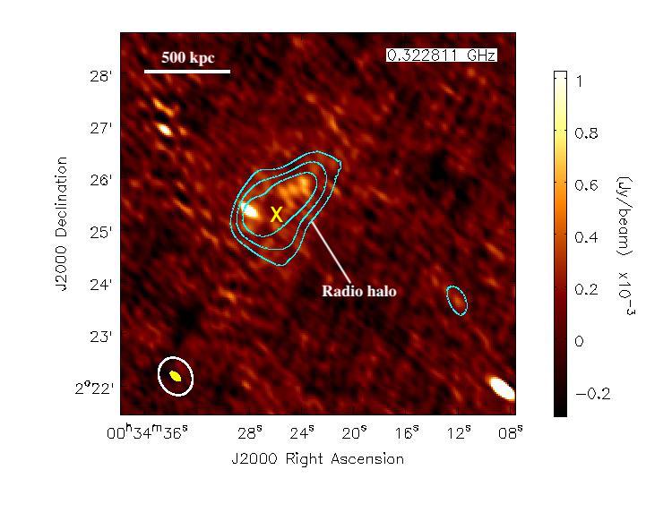
J0034 is at redshift 0.382 and has a mass of = 9.0 1014 M⊙ Hilton et al. (2018). At this cluster redshift, 1′′ corresponds to 5.223 kpc and the luminosity distance is 2057.4 Mpc. Carrasco et al. Carrasco et al. (2017) used data from the FOcal Reducer and low dispersion Spectrograph 2 (FORS2; (Appenzeller et al., 1998)), which is mounted at Very Large Telescope (VLT) to study the galaxy cluster. From their observations they derived that the cluster has a rest-frame velocity dispersion of 713 179 kms-1 and a dynamical mass of (3.37 2.19) 1014 M⊙. MeerKAT L-band observations by K20 indicated that the cluster hosts a candidate radio halo. From their observations, they measured the flux density of the radio halo to be 1.26 0.2 mJy, and it has LLS of 348 kpc.
From our 325 MHz GSB data (PI: Kenda Knowles, ID: 32016), we observe the diffuse emission for the first time at this frequency, and confirm its presence as tentatively detected at 1.16 GHz by K20 (see Figure 5). The emission we detect has a larger extent than that detected in K20 due to the observations being at a lower frequency. The flux density of the detected diffuse emission is 16.77 2.34 mJy, and the LAS is 2.32′ 1.46′, corresponding to a LLS of 726 kpc 459 kpc. We note that the flux density measurements might contain residual emission from the BCG that is embedded in the radio halo. This contamination is accounted for as explained in Section 3.3. Using our results and the 1.16 GHz flux density measurement from K20, we calculated the spectral index of the radio halo and found it to be 2.26 0.32. This indicates that the radio halo is an ultra steep spectrum. We used the spectral index to extrapolate the halo radio power at 1.4 GHz and found it to be (0.60 0.15) 1024 WHz-1. Given the extent of the diffuse emission, the central location, and its regular morphology, we confirm that it falls in the category of radio halos. We also note that the irregular morphology of the emission might be an indication of merger activity, given that this cluster is paired with ACTCL J0034.9+0233 which is at the same redshift with a projected separation of 3.5 Mpc Hilton et al. (2018).
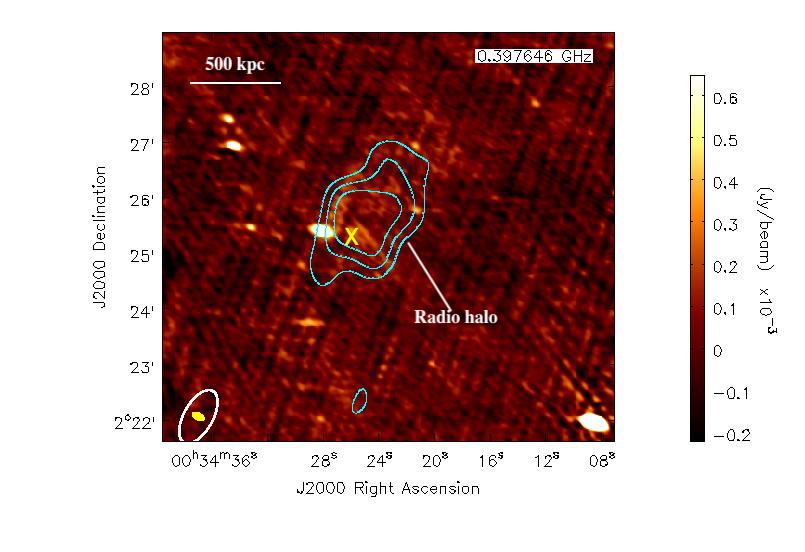
From the GWB data (PI: Kenda Knowles, ID: 32016), we detect extended diffuse emission in the central region of the cluster. We measure the LAS of the diffuse emission to be 2.31′ 1.48′, corresponding to a LLS of 723 kpc 463 kpc. This is similar is size to the GSB detection (LLS 726 459 kpc). The sizes and morphology of the diffuse emission are similar for both the GWB and the GSB images (See Figure 5). Hence, we retain the radio halo classification from the narrowband data analysis.
The flux density of the radio halo for the GWB observations is 6.22 1.64 mJy. We use this value and the 1.16 GHz flux density measurement from K20 to calculate the spectral index of the radio halo. We determine a spectral index of , consistent within the uncertainties of that determined using the GSB measurement. Using our GWB flux density and measured spectral index, we determine a 1.4 GHz radio power of (0.59 0.12) 1024 WHz-1, in agreement with the GSB extrapolated value. We recover the radio halo at a higher SNR in the GWB data. The halo radio power is in agreement for both the GWB and GSB derived values. The morphology of the radio halo in the narrowband image is slightly elongated compared to the wideband image. The difference in morphology could be an indication that the emission at the edge of the halo is faint and hence picked up by the GWB observations, which goes down to frequencies of 250 MHz.
2 \switchcolumn
For this cluster, the GWB data did not significantly add any new scientific information for the radio halo. However, we note that this dataset was severely affected by RFI and DDEs. The bright sources make this field an extreme data reduction challenge and is therefore a good candidate to test future SKA pipelines.
5 Summary and Future Outlook
The sensitivity of new generation telescopes has allowed for the study of diffuse emission in previously unexplored parameter spaces. Recent statistical studies of diffuse radio emission now consist of cluster samples that target lower mass and higher redshift clusters. Such studies are crucial for understanding the cosmological evolution of the diffuse radio sources, their connection to the dynamical state of the host cluster, and for the refinement of the currently existing formation theories.
In this paper, we presented an overview of an SZ-selected ACTPol sample of 40 clusters that spans a wide mass (4.5 1014 M⊙ 10.5) and redshift range (0.15 1.0). We followed up this sample using the GMRT. Seventeen clusters have existing archival GSB observation, and we obtained uGMRT GWB band 3 data for thirteen clusters. We reduced the J0034 GSB data using spam. We then presented the challenges we faced with reducing the GWB data for the complex J0034 field, and the three pipelines we explored. The experimental spam wideband pipeline produced the most improved results. Finally, we used J0034 as a case study to compare the GSB and GWB data analysis results. We found that halo radio power is in agreement for both the GWB and GSB derived values. Although the GWB data did not significantly add any new scientific features for the radio halo, the flux is detected at a higher level. We note that the uGMRT data reduction still needs to be refined to perform in-band spectral index studies.
We note that the current best pipeline for the GWB data is still in the experimental stage and could be optimised to produce better results. The complex J0034 field indicates the need for advanced 3GC technique for the next generation of low frequency and wide bandwidth telescopes. Finally, we aim to carry out statistical studies on the full sample once the narrowband and wideband analysis is completed.
Conceptualization, K.M. and K.K.; methodology, K.M., K.K. and S.P.S.; software, C.H.I.-C. and M.H.; formal analysis, S.P.S.; writing—original draft preparation, S.P.S.; writing—review and editing, M.H., N.G., K.K. and K.M.; supervision, K.M., K.K. and M.H. All authors have read and agreed to the published version of the manuscript.
S.P.S. acknowledges funding from the South African Radio Astronomy Observatory and the National Research Foundation (NRF Grant Number: 95533).
Not applicable
Not applicable
The uGMRT data reported in this paper are available through the GMRT online archive. https://naps.ncra.tifr.res.in/goa. The data were last accessed November 2020. Besides the raw UVFITS data, SPAM pipeline processed GSB images are also available in the GMRT archive. The observation IDs for the gsb and gwb datasets are 8651 and 9434, respectively.
Acknowledgements.
S.P.S. acknowledges funding support from NRF/South African Radio Astronomy Observatory. We thank the staff of the GMRT who made these observations possible. GMRT is run by the National Centre for Radio Astrophysics of the Tata Institute of Fundamental Research. CHIC acknowledges the support of the Department of Atomic Energy, Government of India, under the project 12-R&D-TFR-5.02-0700. \conflictsofinterestThe authors declare no conflict of interest. \printendnotes[custom] \reftitleReferencesReferences
- Large et al. (1959) Large, M.I.; Mathewson, D.S.; Haslam, C.G.T. A High-resolution Survey of the Andromeda Nebula at 408 Mc./S. Nature 1959, 183, 1250–1251. doi:\changeurlcolorblack10.1038/1831250a0.
- Brown and Rudnick (2011) Brown, S.; Rudnick, L. Diffuse radio emission in/around the Coma cluster: beyond simple accretion. Mon. Not. R. Astron. Soc. 2011, 412, 2–12. doi:\changeurlcolorblack10.1111/j.1365-2966.2010.17738.x.
- Bonafede et al. (2020) Bonafede, A.; Brunetti, G.; Vazza, F.; Simionescu, A.; Giovannini, G.; Bonnassieux, E.; Shimwell, T.W.; Brüggen, M.; van Weeren, R.J.; Botteon, A.; et al. The Coma cluster at LOFAR frequencies I: insights into particle acceleration mechanisms in the radio bridge. arXiv 2020, arXiv:2011.08856.
- Sarazin (1988) Sarazin, C.L. Book-Review—X-ray Emissions from Clusters of Galaxies. Sky Telesc. 1988, 76, 639.
- Kravtsov and Borgani (2012) Kravtsov, A.V.; Borgani, S. Formation of Galaxy Clusters. Annu. Rev. Astron. Astrophys. 2012, 50, 353–409. doi:\changeurlcolorblack10.1146/annurev-astro-081811-125502.
- Enßlin et al. (2011) Enßlin, T.; Pfrommer, C.; Miniati, F.; Subramanian, K. Cosmic ray transport in galaxy clusters: Implications for radio halos, gamma-ray signatures, and cool core heating. Astron. Astrophys. 2011, 527, A99. doi:\changeurlcolorblack10.1051/0004-6361/201015652.
- Dennison (1980) Dennison, B. Cosmic Rays in Clusters of Galaxies and the Formation of Extended Radio Halos. Bull. Am. Astron. Soc. 1980, 12, 471.
- Pfrommer et al. (2008) Pfrommer, C.; Enßlin, T.A.; Springel, V. Simulating cosmic rays in clusters of galaxies—II. A unified scheme for radio haloes and relics with predictions of the -ray emission. Mon. Not. R. Astron. Soc. 2008, 385, 1211–1241. doi:\changeurlcolorblack10.1111/j.1365-2966.2008.12956.x.
- Reimer et al. (2003) Reimer, O.; Pohl, M.; Sreekumar, P.; Mattox, J.R. EGRET Upper Limits on the High-Energy Gamma-ray Emission of Galaxy Clusters. Astrophys. J. 2003, 588, 155–164. doi:\changeurlcolorblack10.1086/374046.
- Ackermann et al. (2010) Ackermann, M.; Ajello, M.; Atwood, W.B.; Baldini, L.; Ballet, A.F. Fermi LAT observations of cosmic-ray electrons from 7 GeV to 1 TeV. Phys. Rev. D 2010, 82, 092004. doi:\changeurlcolorblack10.1103/PhysRevD.82.092004.
- Ackermann et al. (2018) Ackermann, M.; Ajello, M.; Albert, A.; Atwood, F. Search for Gamma-Ray Emission from the Coma Cluster with Six Years of Fermi-LAT Data. Astrophys. J. 2016, 819, 149; Erratum in 2018, 860, 85.
- Brunetti and Blasi (2005) Brunetti, G.; Blasi, P. Alfvénic reacceleration of relativistic particles in galaxy clusters in the presence of secondary electrons and positrons. Mon. Not. R. Astron. Soc. 2005, 363, 1173–1187. doi:\changeurlcolorblack10.1111/j.1365-2966.2005.09511.x.
- Brunetti et al. (2017) Brunetti, G.; Zimmer, S.; Zandanel, F. Relativistic protons in the Coma galaxy cluster: First gamma-ray constraints ever on turbulent reacceleration. Mon. Not. R. Astron. Soc. 2017, 472, 1506–1525. doi:\changeurlcolorblack10.1093/mnras/stx2092.
- Pinzke et al. (2017) Pinzke, A.; Oh, S.P.; Pfrommer, C. Turbulence and particle acceleration in giant radio haloes: The origin of seed electrons. Mon. Not. R. Astron. Soc. 2017, 465, 4800–4816. doi:\changeurlcolorblack10.1093/mnras/stw3024.
- Brunetti et al. (2001) Brunetti, G.; Setti, G.; Feretti, L.; Giovannini, G. Particle reacceleration in the Coma cluster: radio properties and hard X-ray emission. Mon. Not. R. Astron. Soc. 2001, 320, 365–378. doi:\changeurlcolorblack10.1046/j.1365-8711.2001.03978.x.
- Feretti et al. (2012) Feretti, L.; Giovannini, G.; Govoni, F.; Murgia, M. Clusters of galaxies: Observational properties of the diffuse radio emission. Astron. Astrophys. Rev. 2012, 20, 54. doi:\changeurlcolorblack10.1007/s00159-012-0054-z.
- Donnert and Brunetti (2014) Donnert, J.; Brunetti, G. An efficient Fokker-Planck solver and its application to stochastic particle acceleration in galaxy clusters. Mon. Not. R. Astron. Soc. 2014, 443, 3564–3577. doi:\changeurlcolorblack10.1093/mnras/stu1417.
- Markevitch et al. (2005) Markevitch, M.; Govoni, F.; Brunetti, G.; Jerius, D. Bow Shock and Radio Halo in the Merging Cluster A520. Astrophys. J. 2005, 627, 733–738. doi:\changeurlcolorblack10.1086/430695.
- Lindner et al. (2014) Lindner, R.R.; Baker, A.J.; Hughes, J.P.; Battaglia, N.; Gupta, N.; Knowles, K.; Marriage, T.A.; Menanteau, F.; Moodley, K.; Reese, E.D.; et al. The Radio Relics and Halo of El Gordo, a Massive = 0.870 Cluster Merger. Astrophys. J. 2014, 786, 49. doi:\changeurlcolorblack10.1088/0004-637X/786/1/49.
- Kale et al. (2015) Kale, R.; Venturi, T.; Giacintucci, S.; Dallacasa, D.; Cassano, R.; Brunetti, G.; Cuciti, V.; Macario, G.; Athreya, R. The Extended GMRT Radio Halo Survey. II. Further results and analysis of the full sample. Astron. Astrophys. 2015, 579, A92. doi:\changeurlcolorblack10.1051/0004-6361/201525695.
- Cassano et al. (2013) Cassano, R.; Ettori, S.; Brunetti, G.; Giacintucci, S.; Pratt, G.W.; Venturi, T.; Kale, R.; Dolag, K.; Markevitch, M. Revisiting Scaling Relations for Giant Radio Halos in Galaxy Clusters. Astrophys. J. 2013, 777, 141. doi:\changeurlcolorblack10.1088/0004-637X/777/2/141.
- Brunetti and Jones (2014) Brunetti, G.; Jones, T.W. Cosmic Rays in Galaxy Clusters and Their Nonthermal Emission. Int. J. Mod. Phys. D 2014, 23, 1430007-98. doi:\changeurlcolorblack10.1142/S0218271814300079.
- Sunyaev and Zeldovich (1972) Sunyaev, R.A.; Zeldovich, Y.B. The Observations of Relic Radiation as a Test of the Nature of X-ray Radiation from the Clusters of Galaxies. Comments Astrophys. Space Phys. 1972, 4, 173.
- Cuciti et al. (2015) Cuciti, V.; Cassano, R.; Brunetti, G.; Dallacasa, D.; Kale, R.; Ettori, S.; Venturi, T. Occurrence of radio halos in galaxy clusters. Insight from a mass-selected sample. Astron. Astrophys. 2015, 580, A97. doi:\changeurlcolorblack10.1051/0004-6361/201526420.
- Cuciti et al. (2021) Cuciti, V.; Cassano, R.; Brunetti, G.; Dallacasa, D.; de Gasperin, F.; Ettori, S.; Giacintucci, S.; Kale, R.; Pratt, G.W.; van Weeren, R.J.; et al. Radio halos in a mass-selected sample of 75 galaxy clusters. II. Statistical analysis. arXiv 2021, arXiv:2101.01641.
- van Weeren et al. (2019) van Weeren, R.J.; de Gasperin, F.; Akamatsu, H.; Brüggen, M.; Feretti, L.; Kang, H.; Stroe, A.; Zandanel, F. Diffuse Radio Emission from Galaxy Clusters. Space Sci. Rev. 2019, 215, 16. doi:\changeurlcolorblack10.1007/s11214-019-0584-z.
- Gitti et al. (2002) Gitti, M.; Brunetti, G.; Setti, G. Modeling the interaction between ICM and relativistic plasma in cooling flows: The case of the Perseus cluster. Astron. Astrophys. 2002, 386, 456–463. doi:\changeurlcolorblack10.1051/0004-6361:20020284.
- Bonafede et al. (2014) Bonafede, A.; Intema, H.T.; Bruggen, M.; Russell, H.R.; Ogrean, G.; Basu, K.; Sommer, M.; van Weeren, R.J.; Cassano, R.; Fabian, A.C.; et al. A giant radio halo in the cool core cluster CL1821+643. Mon. Not. R. Astron. Soc. 2014, 444, L44–L48. doi:\changeurlcolorblack10.1093/mnrasl/slu110.
- Parekh et al. (2021) Parekh, V.; Laganá, T.F.; Kale, R. Substructure analysis of the RXCJ0232.2-4420 galaxy cluster. Mon. Not. R. Astron. Soc. 2021, 504, 610–620. doi:\changeurlcolorblack10.1093/mnras/stab779.
- Jaffe and Rudnick (1979) Jaffe, W.J.; Rudnick, L. Observations at 610 MHz of radio halos in clusters of galaxies. Astrophys. J. 1979, 233, 453–462. doi:\changeurlcolorblack10.1086/157406.
- Enßlin et al. (1998) Enßlin, T.A.; Biermann, P.L.; Klein, U.; Kohle, S. Cluster radio relics as a tracer of shock waves of the large-scale structure formation. Astron. Astrophys. 1998, 332, 395–409.
- Bonafede et al. (2012) Bonafede, A.; Brüggen, M.; van Weeren, R.; Vazza, F.; Giovannini, G.; Ebeling, H.; Edge, A.C.; Hoeft, M.; Klein, U. Discovery of radio haloes and double relics in distant MACS galaxy clusters: clues to the efficiency of particle acceleration. Mon. Not. R. Astron. Soc. 2012, 426, 40–56. doi:\changeurlcolorblack10.1111/j.1365-2966.2012.21570.x.
- Botteon et al. (2016) Botteon, A.; Gastaldello, F.; Brunetti, G.; Dallacasa, D. A shock at the radio relic position in Abell 115. Mon. Not. R. Astron. Soc. 2016, 460, L84–L88. doi:\changeurlcolorblack10.1093/mnrasl/slw082.
- Locatelli et al. (2020) Locatelli, N.T.; Rajpurohit, K.; Vazza, F.; Gastaldello, F.; Dallacasa, D.; Bonafede, A.; Rossetti, M.; Stuardi, C.; Bonassieux, E.; Brunetti, G.; et al. Discovering the most elusive radio relic in the sky: Diffuse shock acceleration caught in the act? Mon. Not. R. Astron. Soc. 2020, 496, L48–L53. doi:\changeurlcolorblack10.1093/mnrasl/slaa074.
- Stuardi et al. (2019) Stuardi, C.; Bonafede, A.; Wittor, D.; Vazza, F.; Botteon, A.; Locatelli, N.; Dallacasa, D.; Golovich, N.; Hoeft, M.; van Weeren, R.J.; et al. Particle re-acceleration and Faraday-complex structures in the RXC J1314.4-2515 galaxy cluster. Mon. Not. R. Astron. Soc. 2019, 489, 3905–3926. doi:\changeurlcolorblack10.1093/mnras/stz2408.
- Bell (1978) Bell, A.R. The acceleration of cosmic rays in shock fronts—II. Mon. Not. R. Astron. Soc. 1978, 182, 443–455. doi:\changeurlcolorblack10.1093/mnras/182.3.443.
- Jones and Ellison (1991) Jones, F.C.; Ellison, D.C. The plasma physics of shock acceleration. Space Sci. Rev. 1991, 58, 259–346. doi:\changeurlcolorblack10.1007/BF01206003.
- Pinzke et al. (2013) Pinzke, A.; Oh, S.P.; Pfrommer, C. Giant radio relics in galaxy clusters: Reacceleration of fossil relativistic electrons? Mon. Not. R. Astron. Soc. 2013, 435, 1061–1082. doi:\changeurlcolorblack10.1093/mnras/stt1308.
- Kang et al. (2017) Kang, H.; Ryu, D.; Jones, T.W. Shock Acceleration Model for the Toothbrush Radio Relic. Astrophys. J. 2017, 840, 42. doi:\changeurlcolorblack10.3847/1538-4357/aa6d0d.
- de Gasperin et al. (2014) de Gasperin, F.; van Weeren, R.J.; Brüggen, M.; Vazza, F.; Bonafede, A.; Intema, H.T. A new double radio relic in PSZ1 G096.89+24.17 and a radio relic mass-luminosity relation. Mon. Not. R. Astron. Soc. 2014, 444, 3130–3138. doi:\changeurlcolorblack10.1093/mnras/stu1658.
- Shimwell et al. (2015) Shimwell, T.W.; Markevitch, M.; Brown, S.; Feretti, L.; Gaensler, B.M.; Johnston-Hollitt, M.; Lage, C.; Srinivasan, R. Another shock for the Bullet cluster, and the source of seed electrons for radio relics. Mon. Not. R. Astron. Soc. 2015, 449, 1486–1494. doi:\changeurlcolorblack10.1093/mnras/stv334.
- van Weeren et al. (2017) van Weeren, R.J.; Andrade-Santos, F.; Dawson, W.A.; Golovich, N.; Lal, D.V.; Kang, H.; Ryu, D.; Brìggen, M.; Ogrean, G.A.; Forman, W.R.; et al. The case for electron re-acceleration at galaxy cluster shocks. Nat. Astron. 2017, 1, 0005. doi:\changeurlcolorblack10.1038/s41550-016-0005.
- Bonafede et al. (2014) Bonafede, A.; Intema, H.T.; Brüggen, M.; Girardi, M.; Nonino, M.; Kantharia, N.; van Weeren, R.J.; Röttgering, H.J.A. Evidence for Particle Re-acceleration in the Radio Relic in the Galaxy Cluster PLCKG287.0+32.9. Astrophys. J. 2014, 785, 1. doi:\changeurlcolorblack10.1088/0004-637X/785/1/1.
- van Weeren et al. (2017) van Weeren, R.J.; Ogrean, G.A.; Jones, C.; Forman, W.R.; Andrade-Santos, F.; Pearce, C.J.J.; Bonafede, A.; Brüggen, M.; Bulbul, E.; Clarke, T.E.; et al. Chandra and JVLA Observations of HST Frontier Fields Cluster MACS J0717.5+3745. Astrophys. J. 2017, 835, 197. doi:\changeurlcolorblack10.3847/1538-4357/835/2/197.
- Zimbardo and Perri (2017) Zimbardo, G.; Perri, S. Superdiffusive shock acceleration at galaxy cluster shocks. Nat. Astron. 2017, 1, 0163. doi:\changeurlcolorblack10.1038/s41550-017-0163.
- Zimbardo and Perri (2018) Zimbardo, G.; Perri, S. Understanding the radio spectral indices of galaxy cluster relics by superdiffusive shock acceleration. Mon. Not. R. Astron. Soc. 2018, 478, 4922–4930. doi:\changeurlcolorblack10.1093/mnras/sty1438.
- Guo et al. (2014) Guo, X.; Sironi, L.; Narayan, R. Non-thermal Electron Acceleration in Low Mach Number Collisionless Shocks. II. Firehose-mediated Fermi Acceleration and its Dependence on Pre-shock Conditions. Astrophys. J. 2014, 797, 47. doi:\changeurlcolorblack10.1088/0004-637X/797/1/47.
- Caprioli and Spitkovsky (2014) Caprioli, D.; Spitkovsky, A. Simulations of Ion Acceleration at Non-relativistic Shocks. III. Particle Diffusion. Astrophys. J. 2014, 794, 47. doi:\changeurlcolorblack10.1088/0004-637X/794/1/47.
- van Haarlem et al. (2013) van Haarlem, M.P.; Wise, M.W.; Gunst, A.W.; Heald, G.; McKean, J.P.; Hessels, J.W.T.; de Bruyn, A.G.; Nijboer, R.; Swinbank, J.; Fallows, R.; et al. LOFAR: The LOw-Frequency ARray. Astron. Astrophys. 2013, 556, A2. doi:\changeurlcolorblack10.1051/0004-6361/201220873.
- Jonas and MeerKAT Team (2016) Jonas, J.; MeerKAT Team. The MeerKAT Radio Telescope. In Proceedings of the MeerKAT Science: On the Pathway to the SKA, Stellenbosch, South Africa, 25–27 May 2016; p. 1.
- Gupta et al. (2017) Gupta, Y.; Ajithkumar, B.; Kale, H.S.; Nayak, S.; Sabhapathy, S.; Sureshkumar, S.; Swami, R.V.; Chengalur, J.N.; Ghosh, S.K.; Ishwara-Chandra, C.H.; et al. The upgraded GMRT: Opening new windows on the radio Universe. Curr. Sci. 2017, 113, 707–714.
- de Gasperin et al. (2017) de Gasperin, F.; Intema, H.T.; Shimwell, T.W.; Brunetti, G.; Brüggen, M.; Enßlin, T.A.; van Weeren, R.J.; Bonafede, A.; Röttgering, H.J.A. Gentle reenergization of electrons in merging galaxy clusters. Sci. Adv. 2017, 3, e1701634. doi:\changeurlcolorblack10.1126/sciadv.1701634.
- Knowles et al. (2019) Knowles, K.; Baker, A.J.; Bond, J.R.; Gallardo, P.A.; Gupta, N.; Hilton, M.; Hughes, J.P.; Intema, H.; López-Caraballo, C.H.; Moodley, K.; et al. GMRT 610 MHz observations of galaxy clusters in the ACT equatorial sample. Mon. Not. R. Astron. Soc. 2019, 486, 1332–1349. doi:\changeurlcolorblack10.1093/mnras/stz823.
- Giovannini et al. (2020) Giovannini, G.; Cau, M.; Bonafede, A.; Ebeling, H.; Feretti, L.; Girardi, M.; Gitti, M.; Govoni, F.; Ignesti, A.; Murgia, M.; et al. Diffuse radio sources in a statistically complete sample of high-redshift galaxy clusters. Astron. Astrophys. 2020, 640, A108. doi:\changeurlcolorblack10.1051/0004-6361/202038263.
- Raja et al. (2021) Raja, R.; Rahaman, M.; Datta, A.; van Weeren, R.J.; Intema, H.T.; Paul, S. A low-frequency radio halo survey of the South Pole Telescope SZ-selected clusters with the GMRT. Mon. Not. R. Astron. Soc. 2021, 500, 2236–2249. doi:\changeurlcolorblack10.1093/mnras/staa3432.
- Venturi et al. (2008) Venturi, T.; Giacintucci, S.; Dallacasa, D.; Cassano, R.; Brunetti, G.; Bardelli, S.; Setti, G. GMRT radio halo survey in galaxy clusters at = 0.2 0.4. II. The eBCS clusters and analysis of the complete sample. Astron. Astrophys. 2008, 484, 327–340. doi:\changeurlcolorblack10.1051/0004-6361:200809622.
- Andrade-Santos et al. (2017) Andrade-Santos, F.; Jones, C.; Forman, W.R.; Lovisari, L.; Vikhlinin, A.; van Weeren, R.J.; Murray, S.S.; Arnaud, M.; Pratt, G.W.; Démoclès, J.; et al. The Fraction of Cool-core Clusters in X-ray versus SZ Samples Using Chandra Observations. Astrophys. J. 2017, 843, 76. doi:\changeurlcolorblack10.3847/1538-4357/aa7461.
- Planck Collaboration et al. (2011) Planck Collaboration; Ade, P.A.R.; Aghanim, N.; Arnaud, M.; Ashdown, M.; Aumont, J.; Baccigalupi, C.; Baker, M.; Balbi, A.; Banday, A.J.; et al. Planck early results. I. The Planck mission. Astron. Astrophys. 2011, 536, A1. doi:\changeurlcolorblack10.1051/0004-6361/201116464.
- Carlstrom et al. (2011) Carlstrom, J.E.; Ade, P.A.R.; Aird, K.A.; Benson, B.A.; Bleem, L.E.; Busetti, S.; Chang, C.L.; Chauvin, E.; Cho, H.M.; Crawford, T.M.; et al. The 10 Meter South Pole Telescope. Publ. Astron. Soc. Pac. 2011, 123, 568. doi:\changeurlcolorblack10.1086/659879.
- Louis et al. (2017) Louis, T.; Grace, E.; Hasselfield, M.; Lungu, M.; Maurin, L.; Addison, G.E.; Ade, P.A.R.; Aiola, S.; Allison, R.; Amiri, M.; et al. The Atacama Cosmology Telescope: two-season ACTPol spectra and parameters. J. Cosmol. Astropart. Phys. 2017, 2017, 031. doi:\changeurlcolorblack10.1088/1475-7516/2017/06/031.
- Hilton et al. (2018) Hilton, M.; Hasselfield, M.; Sifón, C.; Battaglia, N.; Aiola, S.; Bharadwaj, V.; Bond, J.R.; Choi, S.K.; Crichton, D.; Datta, R.; et al. The Atacama Cosmology Telescope: The Two-season ACTPol Sunyaev-Zel’dovich Effect Selected Cluster Catalog. Astrophys. J. Suppl. Ser. 2018, 235, 20. doi:\changeurlcolorblack10.3847/1538-4365/aaa6cb.
- Arnaud et al. (2010) Arnaud, M.; Pratt, G.W.; Piffaretti, R.; Böhringer, H.; Croston, J.H.; Pointecouteau, E. The universal galaxy cluster pressure profile from a representative sample of nearby systems (REXCESS) and the YSZ - M500 relation. Astron. Astrophys. 2010, 517, A92. doi:\changeurlcolorblack10.1051/0004-6361/200913416.
- Knowles et al. (2016) Knowles, K.; Baker, A.J.; Basu, K.; Bharadwaj, V.; de Gasperin, F.; Deane, R.; Devlin, M.; Dicker, S.; Ferrari, C.; Hilton, M.; et al. MERGHERS: An SZ-selected cluster survey with MeerKAT. In Proceedings of the MeerKAT Science: On the Pathway to the SKA, Stellenbosch, South Africa, 25–27 May 2016; p. 30.
- Gupta et al. (2016) Gupta, N.; Srianand, R.; Baan, W.; Baker, A.J.; Beswick, R.J.; Bhatnagar, S.; Bhattacharya, D.; Bosma, A.; Carilli, C.; Cluver, M.; et al. The MeerKAT Absorption Line Survey (MALS). In Proceedings of the MeerKAT Science: On the Pathway to the SKA, Stellenbosch, South Africa, 25–27 May 2016; p. 14.
- Intema (2014) Intema, H.T. SPAM: A data reduction recipe for high-resolution,low-frequency radio-interferometric observations. Astron. Soc. India Conf. Ser. 2014, 13, 469.
- Intema et al. (2017) Intema, H.T.; Jagannathan, P.; Mooley, K.P.; Frail, D.A. The GMRT 150 MHz all-sky radio survey. First alternative data release TGSS ADR1. Astron. Astrophys. 2017, 598, A78. doi:\changeurlcolorblack10.1051/0004-6361/201628536.
- Kettenis et al. (2006) Kettenis, M.; van Langevelde, H.J.; Reynolds, C.; Cotton, B. ParselTongue: AIPS Talking Python. In Astronomical Data Analysis Software and Systems XV; Gabriel, C., Arviset, C., Ponz, D., Enrique, S., Eds.; Astronomical Society of the Pacific Conference Series; San Lorenzo de El Escorial, Spain, 2-5 October 2005; Volume 351, p. 497.
- van Moorsel et al. (1996) van Moorsel, G.; Kemball, A.; Greisen, E. AIPS Developments in the Nineties. In Astronomical Data Analysis Software and Systems V; Jacoby, G.H., Barnes, J., Eds.; Astronomical Society of the Pacific Conference Series; Tucson, Arizona, USA, 23-25 October 1995; Volume 101, p. 37.
- Cornwell and Perley (1992) Cornwell, T.J.; Perley, R.A. Radio-interferometric imaging of very large fields. The problem of non-coplanar arrays. Astron. Astrophys. 1992, 261, 353–364.
- Cohen et al. (2007) Cohen, A.S.; Lane, W.M.; Cotton, W.D.; Kassim, N.E.; Lazio, T.J.W.; Perley, R.A.; Condon, J.J.; Erickson, W.C. The VLA Low-Frequency Sky Survey. Astron. J. 2007, 134, 1245–1262. doi:\changeurlcolorblack10.1086/520719.
- Condon et al. (1998) Condon, J.J.; Cotton, W.D.; Greisen, E.W.; Yin, Q.F.; Perley, R.A.; Taylor, G.B.; Broderick, J.J. The NRAO VLA Sky Survey. Astron. J. 1998, 115, 1693–1716. doi:\changeurlcolorblack10.1086/300337.
- Lonsdale (2005) Lonsdale, C.J. Configuration Considerations for Low Frequency Arrays. In From Clark Lake to the Long Wavelength Array: Bill Erickson’s Radio Science; Kassim, N., Perez, M., Junor, W., Henning, P., Eds.; Astronomical Society of the Pacific Conference Series; Cambridge, Massachusetts, USA, 18-21 June 2005; Volume 345, p. 399.
- Kale and Ishwara-Chandra (2020) Kale, R.; Ishwara-Chandra, C.H. CAPTURE: Interferometric Pipeline for Image Creation from GMRT Data. In Experimental Astronomy 2020, Volume 51, p. 95-108.
- McMullin et al. (2007) McMullin, J.P.; Waters, B.; Schiebel, D.; Young, W.; Golap, K. CASA Architecture and Applications. In Astronomical Data Analysis Software and Systems XVI; Shaw, R.A., Hill, F., Bell, D.J., Eds.; Astronomical Society of the Pacific Conference Series; Austin, Texas, USA 14-16 October 2007; Volume 376, p. 127.
- Perley and Butler (2013) Perley, R.A.; Butler, B.J. An Accurate Flux Density Scale from 1 to 50 GHz. Astrophys. J. Suppl. Ser. 2013, 204, 19. doi:\changeurlcolorblack10.1088/0067-0049/204/2/19.
- Offringa et al. (2012) Offringa, A.R.; van de Gronde, J.J.; Roerdink, J.B.T.M. A morphological algorithm for improving radio-frequency interference detection. Astron. Astrophys. 2012, 539, A95. doi:\changeurlcolorblack10.1051/0004-6361/201118497.
- Tasse et al. (2018) Tasse, C.; Hugo, B.; Mirmont, M.; Smirnov, O.; Atemkeng, M.; Bester, L.; Hardcastle, M.J.; Lakhoo, R.; Perkins, S.; Shimwell, T. Faceting for direction-dependent spectral deconvolution. Astron. Astrophys. 2018, 611, A87. doi:\changeurlcolorblack10.1051/0004-6361/201731474.
- Joye and Mandel (2003) Joye, W.A.; Mandel, E. New Features of SAOImage DS9. In Astronomical Data Analysis Software and Systems XII; Payne, H.E., Jedrzejewski, R.I., Hook, R.N., Eds.; Astronomical Society of the Pacific Conference Series; Princeton, New Jersey, USA, 27-30 July 2003; Volume 295, p. 489.
- Knowles et al. (2016) Knowles, K.; Intema, H.T.; Baker, A.J.; Bharadwaj, V.; Bond, J.R.; Cress, C.; Gupta, N.; Hajian, A.; Hilton, M.; Hincks, A.D.; et al. A giant radio halo in a low-mass SZ-selected galaxy cluster: ACT-CL J0256.5+0006. Mon. Not. R. Astron. Soc. 2016, 459, 4240–4258. doi:\changeurlcolorblack10.1093/mnras/stw795.
- Chandra et al. (2004) Chandra, P.; Ray, A.; Bhatnagar, S. The Late-Time Radio Emission from SN 1993J at Meter Wavelengths. Astrophys. J. 2004, 612, 974–987. doi:\changeurlcolorblack10.1086/422675.
- Knowles et al. (2020) Knowles, K.; Pillay, D.S.; Amodeo, S.; Baker, A.J.; Basu, K.; Crichton, D.; de Gasperin, F.; Devlin, M.; Ferrari, C.; Hilton, M.; et al. MERGHERS Pilot: MeerKAT discovery of diffuse emission in nine massive Sunyaev-Zel’dovich-selected galaxy clusters from ACT. arXiv 2020, arXiv:2012.15088.
- Carrasco et al. (2017) Carrasco, M.; Barrientos, L.F.; Anguita, T.; García-Vergara, C.; Bayliss, M.; Gladders, M.; Gilbank, D.; Yee, H.K.C.; West, M. VLT/Magellan Spectroscopy of 29 Strong Lensing Selected Galaxy Clusters. Astrophys. J. 2017, 834, 210. doi:\changeurlcolorblack10.3847/1538-4357/834/2/210.
- Appenzeller et al. (1998) Appenzeller, I.; Fricke, K.; Fürtig, W.; Gässler, W.; Häfner, R.; Harke, R.; Hess, H.J.; Hummel, W.; Jürgens, P.; Kudritzki, R.P.; et al. Successful commissioning of FORS1—The first optical instrument on the VLT. Messenger 1998, 94, 1–6.