Symmetry-Breaking in Plant Stems

Abstract.

The purpose of this paper is to present a model of a phenomenon of plant stem morphogenesis observed by Cesar Gomez-Campo in 1970. We consider a simplified model of auxin dynamics in plant stems, showing that, after creation of the original primordium, it can represent random, distichous and spiral phyllotaxis (leaf arrangement) just by varying one parameter, the rate of diffusion. The same analysis extends to the $n$-jugate case where $n$ primordia are initiated at each plastochrone. Having validated the model, we consider how it can give rise to the Gomez-Campo phenomenon, showing how a stem with spiral phyllotaxis can produce branches of the same or opposite chirality. And finally, how the relationship can change from discordant to concordant over the course of a growing season.

1. Introduction

1.1. ”As the Twig is Bent,…”

As a student (more than fifty years ago) the senior author came across a popular exposition on the mathematical patterns in phyllotaxis (leaf arrangement) and was fascinated. The Fibonacci numbers, $F_{n}$, are a mathematical sequence that begins with $F_{1}=1$, $F_{2}=2$ and then for $n\geq 2$, $F_{n+1}=F_{n}+F_{n-1}$. So the numbers continue

$$n$$

ad infinitum. That Fibonacci numbers actually occur in phyllotactic structures on pineapples and pine cones and many other plants inspired awe and curiosity about what lay behind it. It seemed that the mechanism must be stable but flexible and therefore probably simple. At that time (1960) so little was known about morphogenesis that insight into the underlying processes seemed pure fantasy. However, things have changed.

1.2. Background

1.2.1. Hofmeister’s Rule

Much has been written about phyllotaxis since Bravais and Bravais initiated its mathematical study in 1837. Being amateurs in botany we have taken the books by Roger V. Jeans ([3], [4]) as authoritative sources for the pre-21^st century literature of phyllotaxis. The major insight of the 21^st century has been the central role of the plant hormone, auxin. Since primordia (points on a stem where new organs are being initiated) tend to distance themselves from each other. This is known as Hofmeister’s Rule (See the website

http://www.math.smith.edu/phyllo/About/math.html

or [5], p.102). It was long thought that primordia must be the source of a hormone inhibiting other primordia. Experiments have shown however, that the hormone auxin, which stimulates cells to grow and reproduce (mitosis), is responsible for Hofmeister’s Rule. A new primordium becomes an auxin sink because it utilizes auxin to build the vascular structure underneath to support its further growth. Auxin is created at various rates in all plant tissues so it is the depletion of auxin near a primordium that inhibits the establishment of new primordia nearby. Since a source of an inhibitory hormone and a sink of a stimulating hormone have essentially the same effect and the same dynamics, we have found it easier to maintain the original model, thinking of a primordium as a source of antiauxin.

1.2.2. The Model of Smith, et al

To be effective, theory requires a dialog with experiment. The field theory of auxin dynamics has been vetted by various laboratory experiments: Surgery and application of hormones known to promote or counter the effects of auxin. In 2004 Smith, et al proposed a mathematical model of a plant stem [7] that we call the SGMRKP model.

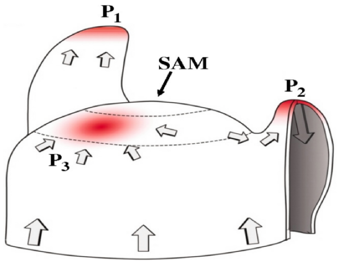
Figure 1. Model of a developing plant stem. P${}_{1},$P${}_{2},$P₃ are primordia.

Most of the morphogenetic activity in a plant stem takes place near the tip, called the meristem and in the outer layer of cells, called the tunica. The tunica is a single layer of cells overlaying the vascular and supporting structure underneath called the phloem. Auxin is created and consumed at various rates in various tissues. At the apex of the tunica is a group of (from 1 to 40) pluripotent (stem) cells called the stem apical meristem (SAM). New organs (primordia) such as leaves or flowers are initiated at points where auxin concentration reaches a critical value. Primordia then absorb auxin from the surrounding tissues in order to build the underlying vascular structure for continued growth. Thus a primordium becomes an auxin sink which inhibits the initiation of other primordia in its immediate vicinity. The SAM itself is a site of growth, extending the stem, and therefore an auxin sink. This means that primordia can only be initiated on its periphery (the peripheral zone). Auxin is transported by diffusion but also actively by cells that are polarized to pump it in one side and out the other. Smith et al proposed a set of equations for auxin dynamics (the SGMRKP model). They were able to solve the equations numerically (on the computer) and create movies of stems growing in various standard phyllotactic patterns - see the website https://www.jic.ac.uk/research-impact/genes-in-the-environment/ of Smith’s group Genes in the Environment at The John Innes Centre. Figure 2 is a photo of a real plant stem, copied from

http://www.cobalt-group.com/frontpagewebs/Content/Classify/

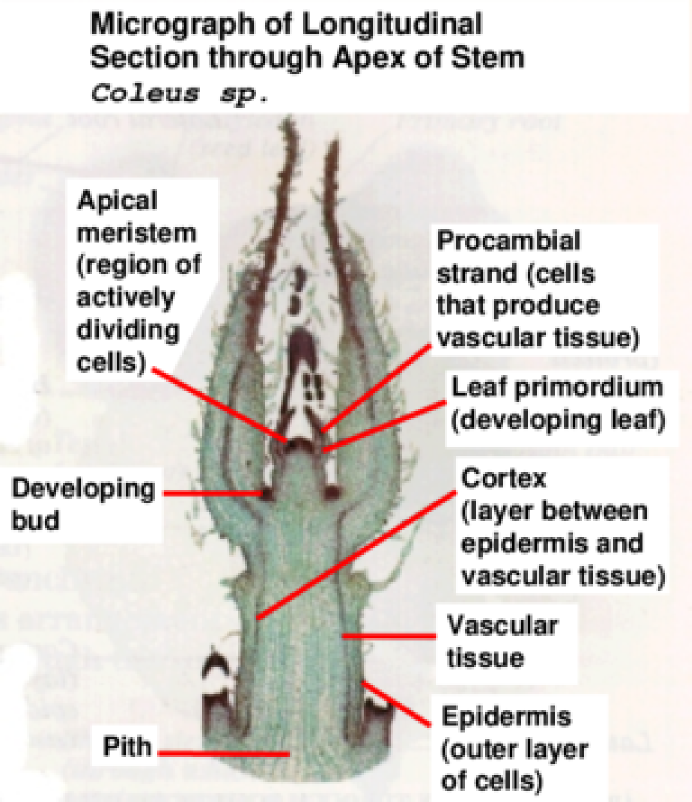
Figure 2. A real plant stem

The SGMRKP model of a growing plant stem leaves out many characteristics of real stems. The hope is that it does capture some vital essence.

1.2.3. Davis’s Hypothesis

The first inkling that the present authors had of being able to make progress in understanding the processes underlying phyllotaxis came circa 1980 from a lecture given in the UCR Mathematics Colloquium by T. Anthony Davis. Dr. Davis was a coconut palm inspector in Kerala Province, India. Inspecting coconut palms (cocos nucifera) was routine work, so Davis began looking into phyllotaxis and noted that, like all plants with spiral phyllotaxis, coconut palms come in two types, left and right handed. Basically, new leaves are formed one at a time in the crown of the tree, each leaf rotated approximately 137.5^∘ from the previous one. If that upward spiral goes to the right, the palm is called right handed. If to the left, left handed. That original arrangement, if left handed, is $(1,2)$ phyllotaxis, the $1$ (genetic) spiral to the left and $2$ spirals of contiguous primordia,called contact parastichies, to the right. If right handed we denote it as $\left(2,1\right)$ phyllotaxis. As a stem grows, the primordia move around to accomodate alterations in proportion and change contiguous neighbors in a systematic way. As a result, the numbers of (left,right) spiraling parastichies changes from ($F_{n-1},F_{n}$) to ($F_{n+1},F_{n}$) (or ($F_{n},F_{n-1}$) to ($F_{n},F_{n+1}$)). Pine cones and pineapples often have ($8,13$) or ($13,8$) phyllotaxy. The genetic spiral will no longer be a contact parastichy, but its direction will be the same as that of the odd order contact parastichies whose numbers are $1,3,8,21$, $55$, etc. A few observations of almost any variety of plant with spiral phyllotaxis will show that both chiralities are possible. Are they then equally probable? What effect does the handedness (chirality) of a palm have on the health & productivity of the tree? Those were the questions with which Dr. Davis entertained himself and claimed to answer: He concluded that they are not equally probable. Of the over 5,000 coconut palms Davis had examined, 51.4% were left handed. By statistics, this was an unlikely event (if the underlying probabilities were equal, 1/2 and 1/2), so the hypothesis (of equality) should be rejected. He went on to gather data from coconut palm inspectors around the world and concluded that those coconut palms in the northern hemisphere were predominantly left handed and those in the southern hemisphere predominantly right handed [1].

2. First Insights

2.1. Vetting Davis’s Hypothesis

Davis’s work was intriguing because if enviromental factors, such as the hemisphere a specimen happens to grow in, could effect chirality, then it opened a window through which morphogenetic processes might be illuminated. And testing of the theory could be done by amateurs! No labs or expensive machinery would be needed. Southern California has lots of palm trees, not coconut palms but why should that make a difference? Also, Riverside is quite a bit further north ($33^{\circ}$) than Kerala Province ($5^{\circ}$ to $15^{\circ\text{)}}$ and that should make the effect even greater (and therefore easier to detect). Furthermore, the discovery of DNA by Crick and Watson in 1953 had set the stage for one of the biggest questions in science today: How does the abstract (digitally encoded) information on DNA get translated into the form and function of a living organism? Though probably a long and complex process, its unraveling will certainly go more quickly if we can pull it apart from both ends. Davis’s hypothesis opened up the possibility of working backward from the end product of development to make inferences about the underlying physico-chemical processes.

The most common local palms, iconic for the Los Angeles area, are Washingtonia Robusta. They are tall (50 to 100 feet) with smooth trunks. This makes it difficult to determine the chirality of their phyllotaxis (a problem that Davis also had to deal with). However, We soon found alternatives in Xylosma Senticosa and bottlebrush (genus Callistemon). Both are plentiful on the UCRiverside campus, their stems have spiral phyllotaxis and chirality is relatively easy to determine. We spent days collecting data and analysing it. We mentored undergrad research projects doing the same. However, the results were not satisfying. Our data consistently indicateded that left handers do predominate but only by a slim margin near Davis’s 51.4%. Davis’s hypothesis implied that the difference should be greater at our lattitude. We thought, ”Maybe the Davis effect requires vertical stems” (Xylosma and bottlebrush stems grow in all directions). So we collected data from lettuce and Washingtonia seedlings (both in a nursery setting). Again, the results were similar except that the more data we collected and the more proficient we became at collecting it, the smaller the predominance of left handers became. Was this an indication of observer bias? Evidently shrinking rejection statistics are common in those areas of science where statistical methods are applied. Professor Robert Rosenthal of the UCR Psychology Department, an expert on this phenomenon, has counciled caution against rejecting the rejection of null hypotheses when shrinking rejection statistics are encountered. Ultimately however, we decided that Davis’s hypothesis was not suitable for our purposes: Even if the chirality of a stem is effected by lattitude, the effect is small and not convenient for amateur experimentation.

2.2. The Gomez-Campo Phenomenon

However, in the course of vetting Davis’s hypothesis, we came upon a way to influence the chirality of a stem that could be useful: In some plants with spiral phyllotaxis (such as bottlebrush, but not palms) the primary stem gives rise to secondary stems (branches). Under certain circumstances a leaf will produce a new stem (called an axillary bud) from the upper side of its base. Secondary stems are functionally the same as primary stems. Does a branch have the same chirality as its parent stem? Again, a few observations on bottlebrush showed that the answer is ”No”. Is the chirality (like that of a primary stem) random (50/50)? A few more observations with bottlebrush showed that the chirality of a branch is the same as that of its parent stem about 2/3 of the time. Following up on this in the library (circa 1982) we found that the phenomenon was already known. A Spanish botanist, Cesar Gomez-Campo, had studied it in 6 annual shrubs in the environs of Madrid and found that the correlation between the chirality of a stem and a branch could even change over the course of the growing season: It could be positive at one time (as it was overall with our bottlebrush) and negative at another [2].

So what mechanism could underly Gomez-Campo’s observations? As before, it had to be stable, yet flexible (and so probably fairly simple). But now it had to be partly deterministic and partly stochastic. This really intrigued us, but again we had no idea as to how to answer the question. Over the years a possible answer slowly took shape: Relative rates of diffusion of auxin interacting with the geometry of the stem. But before we can apply that insight to the Gomez-Campo phenomenon, we need to examine our conceptual model more closely, to clear up an apparent paradox.

2.3. The Paradox of Distichous Phyllotaxis

Hofmeister’s Rule has been the basis for much of the theory of Fibonacci phyllotaxis. In the case where primordia appear one at a time (unijugate phyllotaxy), it implies that the next primordium will appear in the available space (the peripheral zone) at a point farthest from previous ones. This works nicely for spiral phyllotaxis, but what about the distichous phyllotaxis of Clavia (Figure 3), grasses and bird-of-paradise?

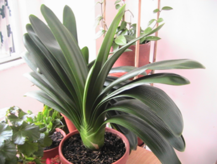
Figure 3. The distichous phyllotaxis of Clavia

In distichous phyllotaxis, two successive leaves on one side appear to be closer to each other than the intermediate one on the other side, apparently contradicting Hofmeister’s Rule. Hofmeister himself ”explained” this by noting that the bases of distichous leaves wrap around the stem to the other side, shielding the following primordium from influence of the leaf preceding it. However we do not find this explanation to be entirely satisfying. Primordia are usually initiated at one point. Why does the base of a distichous leaf extend so much further than in other plants?

2.4. A Quantitative Model

Think of the plant stem as a cylinder of semicircumference 1. A primordium will beome an antiauxin source and we shall assume only diffusion for transport. Let the unit of time (the plastochrone) be the time to the creation of the next primordium and let $\sigma^{2}$ be the variance of the density of antiauxin in the peripheral zone at that time. The normal (Gaussian) density function at time $t$ for diffusion on the real line starting from a unit source at $x_{0}$ is

$$f\left(x;x_{0},\sigma,t\right)=\frac{1}{\sqrt{2\pi t}\sigma}e^{-\frac{\left(x-x_{0}\right)^{2}}{2\sigma^{2}t}}.$$

For $x_{0}=0$, $\sigma=1$ and $t=1$ the graph of this density is the familiar bell-shaped curve (Figure 4).

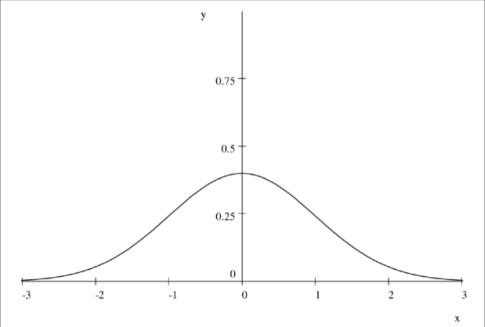
Figure 4. Graph of $f\left(x;0,1,1\right)=\frac{1}{\sqrt{2\pi}}e^{-\frac{x^{2}}{2}}$, $-3<x\leq 3$

The values of $x$ extend mathematically to $\pm\infty$, but according to the table of values for the complimentary error function, erfc (See Wikipedia), the area under the curve for $x>3$ and $x<-3$ is erfc$(3)=2.21\times 10^{-5}$, a negligeable amount.

Diffusion is a linear process, so if we take this same diffusion process and put it on the circle of semicircumference $1$ (the peripheral zone), the tails of the distribution will wrap around and add to give a density of

$$f\left(x;0,1,1\right)+f\left(x;2,1,1\right)+f\left(x;-2,1,1\right),-1<x\leq 1.$$

Higher order wraparounds are negligeable and the graph is displayed in Figure 5.

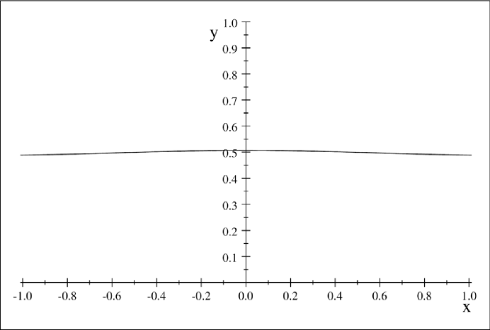
Figure 5. Graph of $f\left(x;0,1,1\right)+f\left(x;2,1,1\right)+f\left(x;-2,1,1\right),$ $-1<x\leq 1$

Somewhat unexpected (but not inconsequential) is that this function is almost constant (near .5). We assume that the placement of the first primordium on a stem is arbitrary. Small random fluctuations in the (theoretically constant) density of antiauxin will determine where it goes. Now if $\sigma=1$ and a second primordium is established one plastochrone after the first, its placement will also be essentially random because the density of antiauxin is again constant, and so on. This accounts for random phyllotaxy (Again, see [5] p. 102), a phenomenon that we had previously ignored because it seemed to ”lack structure” and contradict Hofmeister’s Rule.

2.4.1. Distichous Phyllotaxy

If we start with a density that has $\sigma=1/2$ on the same circle (of semicircumference $1$) we get a density function,

$$\frac{2}{\sqrt{2\pi}}\left(e^{-2x^{2}}+e^{-2\left(x-2\right)^{2}}+e^{-2\left(x+2\right)^{2}}\right),-1\leq x\leq 1,$$

whose graph is Figure 6

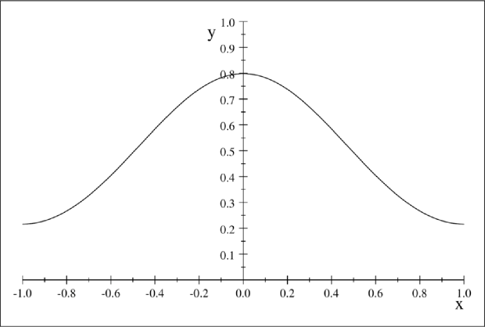
Figure 6. Density on the circle with $\sigma=1/2$

Unlike the case $\sigma=1$, this distribution (of antiauxin) has a definite minimum at $x=\pm 1$, the antipode of $x=0$. After one unit of time (the plastichrone) a 2^nd primordium is created at $\pm 1$. If we recenter Figure 6, translating in $x$ to bring the minimum back to the origin, then after another unit of time the density will be

$$\frac{2}{\sqrt{2\pi}}\left(e^{-2x^{2}}+e^{-2\left(x-2\right)^{2}}+e^{-2\left(x+2\right)^{2}}\right)$$

$$+\frac{1}{\sqrt{\pi}}\left(e^{-\left(x+1\right)^{2}}+e^{-\left(x-1\right)^{2}}+e^{-\left(x+3\right)^{2}}+e^{-\left(x-3\right)^{2}}\right),$$

whose graph is Figure 7.

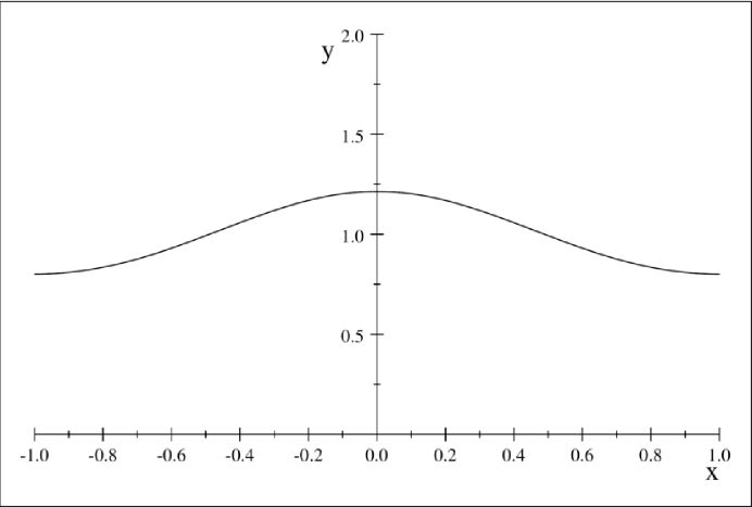
Figure 7. $\sigma=1/2$ density after 2^nd primordium

So there is still a definite minimum at $\pm 1$. If we add a $3^{rd}$ primordium at that minimum and rotate again, after another unit of time the distribution will be

$$\frac{2}{\sqrt{2\pi}}\left(e^{-2x^{2}}+e^{-2\left(x-2\right)^{2}}+e^{-2\left(x+2\right)^{2}}\right)$$

$$+\frac{1}{\sqrt{\pi}}\left(e^{-\left(x+1\right)^{2}}+e^{-\left(x-1\right)^{2}}+e^{-\left(x+3\right)^{2}}+e^{-\left(x-3\right)^{2}}\right)$$

$$+\frac{2}{\sqrt{6\pi}}\left(e^{-2\left(x+2\right)^{2}/3}+e^{-2x^{2}/3}+e^{-2\left(x-2\right)^{2}\backslash 3}\right)\text{,}$$

whose graph is Figure 8.

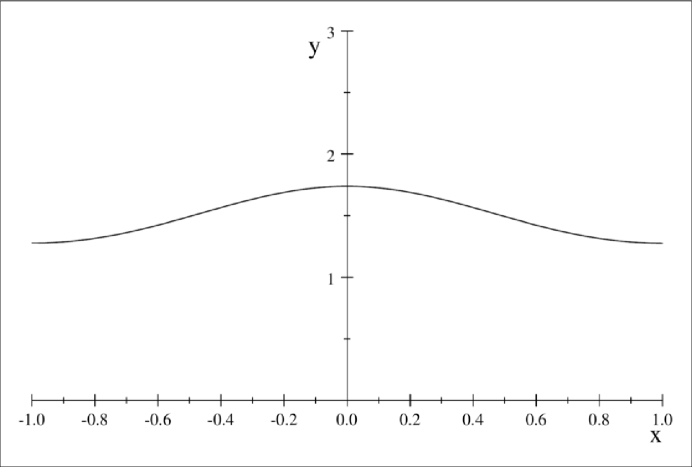
Figure 8. $\sigma=1/2$, density after $3^{rd}$ primordium

And the minimum is still at $x=\pm 1$. In fact the whole curve is much the same as the previous curve, except that each point is higher (by about .$5$). This is due to the fact that the distribution of antiauxin from the first primordium has diffused to that of Fig. 5. The additional antiauxin will presumably be absorbed. We see that repetitions of this process will give essentially the same result, which is to say, the process is stable. This represents distichous phyllotaxy. This stable distribution of antiauxin is not flat as it was for $\sigma=1$, but flatter than it will be for smaller $\sigma$, a possible explanation for the wraparound feature of distichous leaves.

2.4.2. Spiral Phyllotaxy

If $\sigma=1/4$, the 2^nd primordium will again be at $\pm 1$ but for the 3^rd the situation is qualitatively different (Figure 9): There are two minima at $\pm.506$

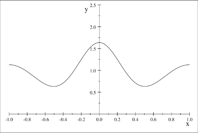
Figure 9. $\sigma=1/4$, density after 2^nd primordium

If we (arbitrarily) choose the positive minimum for the third primordium (starting a right-handed spiral) and rotate it back to the origin, after another plastochrone the density of antiauxin will be essentially

$$\frac{4}{\sqrt{2\pi}}e^{-8x^{2}}+\frac{2}{\sqrt{\pi}}\left(e^{-4\left(x+.505\right)^{2}}+e^{-4\left(x-1.495\right)^{2}}\right)$$

$$+\frac{4}{\sqrt{6\pi}}\left(e^{-8\left(x+1.505\right)^{2}/3}+e^{-8\left(x-.495\right)^{2}/3}\right)$$

whose graph is Figure 9.

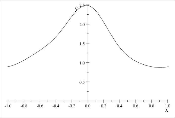
Figure 10. $\sigma=1/4$, density after 3^rd primordium

So, the (now unique) minimum is at $x_{3}=$ $.903$, continuing the right-handed spiral. After another plastochrone the density is Figure 10.

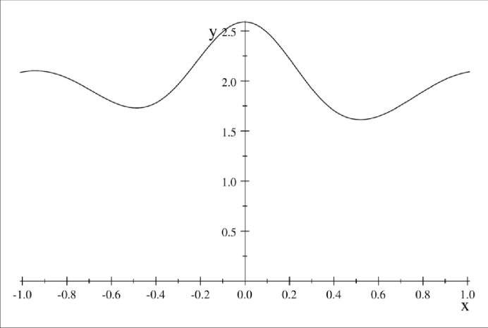
Figure 11. $\sigma=1/4$, density after 4^th primordium

So, the minimum is at $x_{4}=$ $.519$. The value $x_{k}$ is a measure of what botanists call the divergence angle of the $k^{th}$ primordium (the angle that it is turned from the previous primordium). Continuing on in this way we obtained a sequence of divergence angles, the first 22 of which are: 1, .505, .903, .519, .884, .534, .841, .546, .802, .560, .749, .577, .692, .596, .650, .611, .630, .618, .625, .620, .623, .622. They then remain .622 (rounded off to 3 decimal places to $n=30$ where we halted the computation. For all practical purposes these values are convergent. This represents spiral phyllotaxis. We shall return to the question of asymptotic convergence of the divergence angles in Section 3.

The Smith et al model of morphogenesis given in [7] is a caricature of reality. Our model is a caricature of their caricature. It’s simplicity however, allows us to analyse it with calculus. It is not adequate to account for the creation of the initial primordia. As was recognized by Alan Turing [8], the initiation of primordia de novo requires a reaction that liberates energy. But does our simplified model retain some essence of reality? Can it account for the placement of subsequent primordia and their qualitative properties?

2.5. Where Does Slow Diffusion Leave Off and Fast Diffusion Begin?

We have seen in the previous examples that if $\sigma$ is large ($\geq 1/2$) the antiauxin density one plastochrone after the placement of the $k^{th}$ primordium will have only one minimum, right on top of the $(k-1)^{st}$ primordium. The $(k+1)^{st}$ primordium goes at that minimum and we have a model of distichous phyllotaxy. On the other hand, if $\sigma$ is small ($\leq 1/4$), one plastochrone after the $2^{nd}$ primordium the density function has two symmetrical minima, each of which will (with probability $1/2$) be the site of the 3^rd primordium. This random choice initiates a left- or right-handed spiral which subsequent placements continue. These constitute the two kinds of mirror symmetric spiral phyllotaxy.

Evidently some $\sigma_{0}$, $1/4<\sigma_{0}<1/2$, is a critical point between where the graph of auxin density at time 2 is concave down at $x=\pm 1$ and where it is concave up. Taking $x=+1$ to represent $x=\pm 1$, this means (since higher order wraparounds are negligeable) that $F(\sigma)=$

$$\frac{\partial^{2}(f(1;0,\sigma,1)+f(1;2,\sigma,1)+f(1;1,\sigma,2)+f(1;-1,\sigma,2))+f(1;3,\sigma,2)}{\partial x^{2}}$$

$$<0\text{ for }\sigma<\sigma_{0}$$

and

$$F(\sigma)>0\text{ for }\sigma>\sigma_{0}\text{.}$$

Thus we must solve $F(\sigma)=0.$ Now

$$f(x;x_{0},\sigma,t)=\frac{1}{\sqrt{2\pi t}\sigma}e^{-\left(x-x_{0}\right)^{2}/2\sigma^{2}t}$$

so

$$\frac{\partial f(x;x_{0},\sigma,t)}{\partial x}=\frac{1}{\sqrt{2\pi t}\sigma}\frac{\partial e^{-\left(x-x_{0}\right)^{2}/2\sigma^{2}t}}{\partial x}=-\frac{1}{\sqrt{2\pi t^{3}}\sigma^{3}}\left(x-x_{0}\right)e^{-\left(x-x_{0}\right)^{2}/2\sigma^{2}t}$$

and

$$\frac{\partial^{2}f(x;x_{0},\sigma,t)}{\partial x^{2}}=\frac{1}{\sqrt{2\pi t^{5}}\sigma^{5}}\left[\left(x-x_{0}\right)^{2}-\sigma^{2}t\right]e^{-\left(x-x_{0}\right)^{2}/2\sigma^{2}t}\text{.}$$

Therefore, since $f(x;x_{0},\sigma,t)$ is symmetric about $x_{0}$ and only depends on $x-x_{0}$,

$$F(\sigma) =2\frac{\partial^{2}(f(1;0,\sigma,1)}{\partial x^{2}}+\frac{\partial^{2}(f(1;1,\sigma,2)}{\partial x^{2}}+2\frac{\partial^{2}(f(1;3,\sigma,2)}{\partial x^{2}}$$

$$=\frac{1}{\sqrt{2\pi}\sigma^{5}}\left[2\left(1-\sigma^{2}\right)e^{-1/2\sigma^{2}}+\frac{1}{2^{5/2}}\left(\left(-2\sigma^{2}\right)+2\left(2^{2}-2\sigma^{2}\right)e^{-2^{2}/2\cdot 2\sigma^{2}}\right)\right]$$

$$=\frac{2}{\sqrt{2\pi}\sigma^{5}}\left[\left(1-\sigma^{2}\right)e^{-1/2\sigma^{2}}+\frac{1}{2^{5/2}}\left(-\sigma^{2}+\left(2^{2}-2\sigma^{2}\right)e^{-1/\sigma^{2}}\right)\right]$$

$$=\frac{2^{-3/2}e^{-1/\sigma^{2}}}{\sqrt{2\pi}\sigma^{5}}\left[2^{5/2}\left(1-\sigma^{2}\right)e^{1/2\sigma^{2}}-\sigma^{2}e^{1/\sigma^{2}}+2\left(2-\sigma^{2}\right)\right]$$

So letting $s=\sigma^{2}$ we wish to solve

$$4\sqrt{2}\left(1-s\right)e^{1/2s}-se^{1/s}+2\left(2-s\right)=0$$

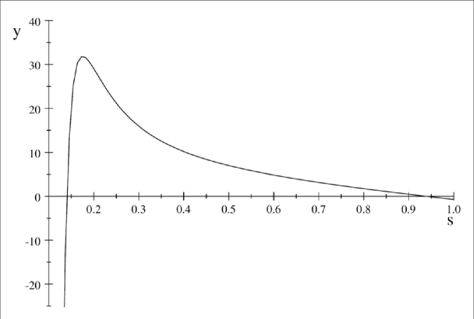
Figure 12. The graph of $y=4\sqrt{2}\left(1-s\right)e^{1/2s}-se^{1/s}+2\left(2-s\right)$

and we see that $s_{0}$, the root we are looking for, is around $0.14$. Our calculation showed that $s_{0}$ is exactly $0.140$ to 3 decimal places, so $\sigma_{0}=\sqrt{.140}=\allowbreak 0.374\,$ and $\frac{1}{3}<\sigma_{0}<\frac{1}{2}$ as we had surmised earlier. Note that the change of $F(\sigma)$ near $\sigma_{0}$ is precipitous.

3. The Range of Divergence Angles

3.1. For Small $k$

Here is a table of divergence angles from various sources for values of $k$, the number of primordia on a stem:

$k$	$1$	$2$	$3$	$4$	$5$	$6$	$7$	$8$	$9$	$10$	…	$\infty$
Arab.	$-$	$170$	$108$	$158$	$127$	$145$	$130$	$135$	$132$	$133$	…	$137.5$
SGMRKP	$-$	$160$	$108$	$157$	$125$	$143$	$140$	$130$	$142$	$123$	…
$\sigma=1/4$	$-$	$180$	$91$	$162$	$93$	$159$	$98$	$152$	$98$	$144$	…	$112$
$\ \sigma=1/3$	$-$	$180$	$119$	$146$	$122$	$141$	$128$	$136$	$130$	$134$	…	$132$

The first row, taken from the paper by Smith et al [7], shows divergence angles measured in Arabadopsis Thaliana, the standard subject for laboratory botanical experiments. The values are averages with standard deviations from $8^{\circ}$ for $k=2$ and increasing up to $20^{\circ}$. The second row, also from [7], is the result of a calculation with the SGMRKP (computer-based) model of spiral phyllotaxis. The third and fourth rows are results of our calculations with the purely diffusive model. $\sigma=1/4$ was the calculation we ran through in Section 2.4.2 but converted to degrees. Since the calculation of the previous section showed that $\sigma=1/3<\sigma_{0}$ still gives spiral phyllotaxis, we calculated the sequence of divergence angles for it also. Some observations:

1. The agreement between rows 1 (Arabadopsis) and 2 (the SGMRKP computational model) is quite good for $3\leq k\leq 6$, but then they drift apart.

2. Row 4 ($\sigma=1/3$) is not so close to row 1 (arabadopsis) at the beginning but their agreement for $k\geq 7$ is striking. Smith et al state that the divergence angle for Arabadopsis converges to the Fibonacci Angle ($360/\tau^{2}\simeq 137.5^{\circ}$where $\tau=\left(1+\sqrt{5}\right)/2$, the Golden Mean (See [3])). However row $4$ converges to $132^{\circ}$ and the coconvergence of rows 1 & 4 make it seem likely that the limit of row 1 is more like 132.5^∘. The claim that row 1 converges to $137.5^{\circ}$ may be a misuse of the mathematical theorem that the Fibonacci angle ”ensures an equitable allocation of space (for the organs in spiral phyllotaxis)” [4], p. 410. It is true that divergence angles tend to cluster about the Fibonacci angle and and the classical examples, the pine cone and sunflower capitulum, have divergence angles very close to $137.5^{\circ}$. For many other examples however (such as the Arabadopsis stem), where space is not scarce enough to apply selective pressure, divergence angles vary widely.

3. In row 1 (Arabadopsis) the first angle should be about $180^{\circ}$ (assuming Davis’s hypothesis is not valid and there is no environmental (or intrinsic developmental) factor biasing the placement of the second primordium to either side. In our calculations (rows 4 & 5) there is no stochastic component so this is the exact value. Smith et al evidently took the the divergence angle for the second primordium to be the length of the shortest arc between the two. This is not unreasonable but it does distort the underlying stochastic process a bit. In our pure model, since the placement of the second primordium does not break mirror symmetry, the handedness of the stem is determined by the third primordium. We arbitrarily chose it to be on the right side, thus establishing a right-handed spiral. For Arabadopsis the distribution of the first divergence angle is likely to be a normal distribution with mean $180^{\circ}$ and standard deviation of about $13^{\circ}$ (judging from the standard deviations given for the other measurements). The standard deviation given for that first divergence angle in row 1 ($8^{\circ}$) is considerably less than for all the other measurements. If the angles had been measured in the positive sense (thereby allowing angles greater than $180^{\circ}$), and they are normally distributed about $180^{\circ}$, their mean deviation from $180^{\circ}$ would be about $\left(\sqrt{\frac{\pi}{2}}\times\left(180-170\right)\right)^{\circ}=\allowbreak 12.\,\allowbreak 533^{\circ}$. Also, their standard deviation would be about$\frac{8}{\sqrt{1-\frac{2}{\pi}}}^{\circ}=\allowbreak 13.\,\allowbreak 271^{\circ}$ (See Appendix for derivations of these formulas). These inferences seem consistent with the measurements.

4. If row 1 had been started with $180^{\circ}$ (the likely average by symmetry) instead of $170^{\circ}$, its agreement with row 4 would be even more striking. We could also increase $\sigma$ a bit in row 4 to make the limiting divergence angles coincide with $132.5^{\circ}$.

5. As pointed out in the previous remark (4), there is impressive agreement between data from real plants and our simplified model in at least one case (Arabadopsis & $\sigma=1/3+$). The diffusion-only model captures the initial oscillatory behavior of divergence angles as well as their eventual convergence even better than the presumably more realistic model of Smith et al. Note that row 2 (SGMRKP) does not reliably oscillate nor approach a limit.

6. In the beginning we assumed that the underlying diffusion process was 1-dimensional (confined to the periphery of the SAM). One might object to this assumption since the tunica is 2-dimensional and the stem as a whole is 3-dimensional and auxin might well diffuse into those surrounding tissues. We repeated the foregoing calculations with 2-&3-dimensional diffusions (replacing $t$ by $t^{2}$ & $t^{3}$) and found that the results(oscillatory behavior, limiting behavior) were qualitatively the same. The value of $\sigma$ that produced a given limit divergence angle differed slightly from dimension to dimension but at this point $\sigma$ has no physical reality anyway. If at some future time $\sigma$ can be measured, then we may have to modify the dimensionality of the diffusion. Another justification for the 1-dimensional model, besides its simplicity, is that it is the limit of the 2-dimensional model as internodal distances go to 0, and many plants do have small (compared to the semicircumference) internodal distance (for definition see [4] pg. 250 or Wikipedia).

3.2. Limit Divergence Angles as a Function of $\sigma$

In the preceding table we listed limit divergence angles for $\sigma=1/4$ and $1/3$. Calculating limit divergence angles for $.1\leq\sigma\leq.9$ in the same way and plotting them we obtain the graph in Figure 13

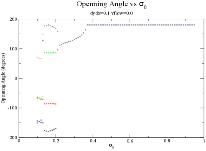
Figure 13. Limit divergence angles

As expected, for $\sigma>\sigma_{0}=.374$ the limit divergence angles are all $180^{\circ}$. For $\sigma<.25$ a kind of instability occurs, so there is no limit for divergence angles but 4 different accumulation points. We have not yet looked into this phenomenon but feel it is related to multijugate phyllotaxis (next section). As mentioned earlier, the limiting divergence for $\sigma=1/4$ is 112^∘. Over the interval $.25\leq\sigma\leq.374$ the limit divergence angle is smoothly increasing from 112^∘ to 180${}^{\circ}.$

In Chapter 27 of [4], Meinhardt, Koch & Bernasconi consider a reaction-diffusion model of phyllotaxis. Their setup is similar to ours: The basic ingredients being an activator, $a$ (auxin?) and two antagonists, $h$ and $s$, interacting in the peripheral zone of the SAM. In Chapter 18, Section 4 of [4], Koch, Bernasconi & Rothen elaborate on this model. Figure 9 of the latter article shows a plot of limit divergence angles as a function of the diffusion constant of $a$. It looks similar to the plot above, even though produced by a somewhat different model. However, there are also quantitative differences: Their curve also splits into 4 branches below .25, but the main one goes to the golden angle (137.5^∘) as the diffusion constant $a$ decreases to 0. Also, the critical value of the diffusion constant (above which the diffusion angle is 180^∘) is about 1 (compared to our $\sigma_{0}=.374$). Their scaling is different (the perimeter of the peripheral region being 1 rather than 2) but this only makes the difference greater. Anyway, these independent calculations reinforce what we found in repeating our calculations many times with different parameters: The qualitative properties of divergence angles are stable under a variety of reasonable assumptions. Our simple model participates in this conscensus and agrees qualitatively with observations of plants.

4. Multijugate Phyllotaxis

$n$-Jugate phyllotaxis starts with $n$ primordia, equally spaced around the peripheral zone and continues in that way at each successive plastochrone. Decussate is the 2-jugate analog of distichous: At each plastochrone two more primordia appear, their axis at a right angle to that of the previous two. Can there be 2-jugate or $n$-jugate spiral phyllotaxis? Most certainly, and they can be represented with the same machinery we used for the unijugate case. The only difference is that we specify the creation of $n$ primordia at each plastochrone. $\sigma$ must then be divided by $n$ and the resulting divergence angles will also be divided by $n$.

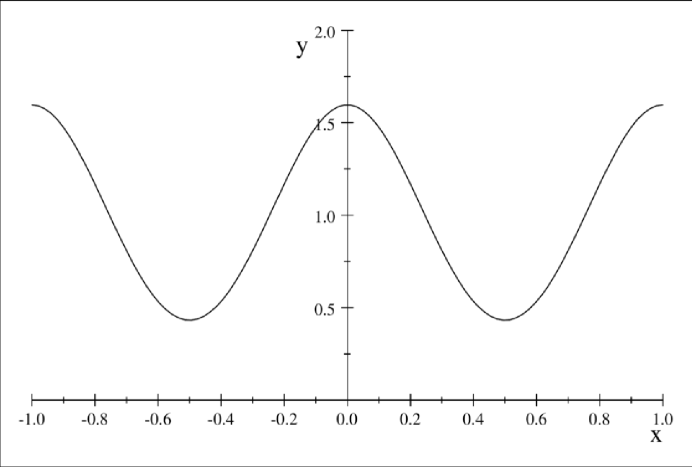
Figure 14. A bijugate distribution for $\sigma=1/4$

Do the bases of decussate (or more generally n-cussate) leaves completely encircle the stem? They do seem to in the few cases we have examined. However, the bases of $n$-jugate spiral leaves cannot, if phyllotaxis is the result of auxin dynamics, since that would block the flow of auxin. However, as we showed in Section 2.4.1, it is not necessary for the bases of n-cussate leaves to encircle their stem. It would be interesting to know if there are any such and if not, why not?

5. The Chirality of Branches

Now we address the question that motivated this project: How is the asymmetry of a stem passed on to a branch? Can auxin dynamics account for the fact that, in a plant with spiral phyllotaxis, an axillary branch may have the same or the opposite chirality as its parent stem? And that the correlation between the two may be positive or negative? Figure 15 copies a graph from the paper by Gomez-Campo [2] showing the correlation between the handedness of a branch at the axil of the $k^{th}$ prophyll and that of its parent stem in the annual plant Hirschfeldia incana:

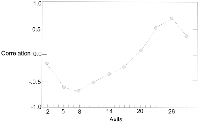
Figure 15. Gomez-Campo’s correlation data

We see a sinuous curve over the course of the growing season. It starts slightly negative ($-0.2$) for the early branches, becomes more negative reaching a minimum of $-0.7$ at $k=8$. It then increases, passing through $0.0$ at $k=19$, reaching a maximum of $0.7$ at $k=26$ and dropping back to $0.4$ at $k=29$. Previous authors had noted isolated correlations ranging from $-1.0$ to $1.0$ and values in between, but Gomez-Campo was the first to record a systematic change over time. At first this lability of corellation might seem surprising since the handedness of stems is so unchanging with time (exceptions have been observed, due to injury of the SAM or seasonal dormancy). Gomez-Campo suggested that correlations could vary over time because of the varying inhibitory influence of successor prophylls. Our model gives quantitative substance to this idea.

First we must look more closely at the physiology of axillary branches. A branch is physiologically the same as a stem. It has a SAM (we call it SAM_k if it is at the base of the $k^{th}$ leaf primordium (prophyll P_k)), beginning with a few pluripotent cells that break off from the SAM of the stem when P_k separates from the peripheryl zone. They stick to the upper edge of the prophyll but do not develop, probably because the prophyll is using up all the auxin. At some instant (time $t_{k}$ for SAM_k) sufficient auxin becomes available (maybe because the prophyll P_k completes its growth or the SAM of the stem is excised) and the branch begins to grow. We posit that the gradient of the antiauxin density at P_k at time $t_{k}$ influences the chirality (right or left) of the branch. This is based on the following observations and assumptions:

1. The base diameter of the branch is relatively small compared to the stem diameter at P_k. Therefore, any influence that the stem might have on auxin concentrations in the branch will be mediated by the gradient of the auxin concentration at P_k.

2. The incipient branch already has a prophyll, P${}_{k,1}=$ P_k, on the lower side of its base so its second prophyll, P_k,2 will be on the upper side of the branch. For our model of a stem, the second prophyll is exactly 180^∘ from the first so it is only the third prophyll whose placement breaks the symmetry and determines whether the stem is right- or left-handed. However, the placement of real stems have a stochastic component, so if the placement of a second prophyll differs significantly from 180^∘ it may already determine the handedness of the stem. The same, of course, holds for branches but there is another factor, the influence of other prophylls, P_j, which may skew the distribution.

3. Assume that our stem has right-handed spiral phylotaxis. If the horizontal gradient of the antiauxin density at P_k is positive at the moment when its axillary bud starts to grow, that will induce a positive gradient across the base of the branch (as viewed from P_k,1). That positive gradient will be promulgated out to the second primordium on the branch and will tend to push P_k,2 to the left. If so the spiral will be left-handed more than half the time, so stem and branch will be discordant. The larger the gradient, the more likely the branch to be discordant. If, on the other hand, the gradient is negative, the branch will tend to be concordant. For left-handed stems the situation is the mirror image of that for right-handed stems and probabilities of concordance and discordance are the same.

4. In our model, when P_k is established (at plastichrone $k$ by definition) the derivative of the horizontal concentration of antiauxin is $0.0$ since P_k is placed at a minimum of antiauxin concentration. At that time, P${}_{k}=$ P_k,1 becomes a source of antiauxin which diffuses away symmetrically. Therefore the derivative of antiauxin concentration will remain $0.0$. As the antiauxin sources at P_j, $j<k$, age out, the antiauxin concentration at P_k may change a bit but it, and its derivative, will remain close to $0.0$. This heuristic conclusion has been validated computationally.

5. However, after its initiation at plastochrone $k+1$, $P_{k+1},$ will exert a nontrivial influence on the antiauxin concentration near $P_{k}$. If the stem is right-handed, the gradient of the antiauxin concentration at $P_{k}$ due to $P_{k+1}$ will be positive (since the divergence angle is strictly between $0.0$ and $1.0$ ($0.0$ and 180^∘).

6. The second successor, $P_{k+2}$, will generally have a negative divergence angle (from $P_{k}$) of absolute value less than that of $P_{k+1}$. So $P_{k+2}$, though further from $P_{k}$ vertically, will be closer horizontally. The combined effect (the sum of the derivatives) may be positive or negative depending on the geometry and the timing. That is, qualitatively, the explanation for Gomez-Campo’s observations.

5.1. The Quantitative Model

We don’t know much about Hirschfeldia Incana, so let us use the convenient value $\sigma=1/3$, which gives a limit divergence of $132/180=\allowbreak 0.733\,$ (from Section 3.1). The delay, $d$, will be the time (in plastochrones) between the establishment of $P_{k}$ and $t_{k}$ (when $S_{k}$ starts growing). Implicit in our simplifying assumption of a fixed (limit) divergence is that $k$ is fairly large. So what will be the gradient of the antiauxin density at $P_{k}$ at time $t_{k}=k+d$ be? From our assumptions it is only a function of $d$. For $0\leq d<1$ we have argued above (4) that it will be essentially zero. At $d=1$ the influence of the antiauxin source at $P_{k+1}$ will begin to be felt. For $1\leq d<2$ (assuming that the contributions for all $P_{j}$, $j<k$, remain negligeable, the gradient of the antiauxin density at $P_{k}$ will be

$$\frac{1}{\sqrt{2\pi}}\frac{.733}{\left(1/3\right)^{3}\left(d-1\right)^{3/2}}\left(e^{-\frac{\left(.733\right)^{2}}{2\left(1/3\right)^{2}\left(d-1\right)}}\right)-\frac{1}{\sqrt{2\pi}}\frac{2-.733}{\left(1/3\right)^{3}\left(d-1\right)^{3/2}}\left(e^{-\frac{\left(2-.733\right)^{2}}{2\left(1/3\right)^{2}\left(d-1\right)}}\right)\text{.}$$

The first term is the direct diffusion from $P_{k+1}$ to $P_{k}$, the second is the wraparound. All other wraparounds are negligeable.

For $2\leq d<3$ we have the same formula for the contribution from $P_{k+1}$ plus the contribution from $P_{k+2}$. The total is

$$\frac{1}{\sqrt{2\pi}}\frac{.733}{\left(1/3\right)^{3}\left(d-1\right)^{3/2}}\left(e^{-\frac{\left(.733\right)^{2}}{2\left(1/3\right)^{2}\left(d-1\right)}}\right)-\frac{1}{\sqrt{2\pi}}\frac{2-.733}{\left(1/3\right)^{3}\left(d-1\right)^{3/2}}\left(e^{-\frac{\left(2-.733\right)^{2}}{2\left(1/3\right)^{2}\left(d-1\right)}}\right)$$

$$-\frac{1}{\sqrt{2\pi}}\frac{2-2\left(.733\right)}{\left(1/3\right)^{3}\left(d-2\right)^{3/2}}\left(e^{-\frac{\left(2-2\left(.733\right)\right)^{2}}{2\left(1/3\right)^{2}\left(d-2\right)}}\right)+\frac{1}{\sqrt{2\pi}}\frac{2\left(.733\right)}{\left(1/3\right)^{3}\left(d-2\right)^{3/2}}\left(e^{-\frac{\left(2\left(.733\right)\right)^{2}}{2\left(1/3\right)^{2}\left(d-2\right)}}\right)\text{.}$$

Again, the first new term is the direct diffusion (this time from the left, so it is negative) and the second the wraparound.

For $3\leq d<4$ we have the same formula for the contribution from $P_{k+1}$ and $P_{k+2}$ plus the contribution from $P_{k+3}$. The total is

$$\frac{1}{\sqrt{2\pi}}\frac{.733}{\left(1/3\right)^{3}\left(d-1\right)^{3/2}}\left(e^{-\frac{\left(.733\right)^{2}}{2\left(1/3\right)^{2}\left(d-1\right)}}\right)-\frac{1}{\sqrt{2\pi}}\frac{2-.733}{\left(1/3\right)^{3}\left(d-1\right)^{3/2}}\left(e^{-\frac{\left(2-.733\right)^{2}}{2\left(1/3\right)^{2}\left(d-1\right)}}\right)$$

$$-\frac{1}{\sqrt{2\pi}}\frac{2-2\left(.733\right)}{\left(1/3\right)^{3}\left(d-2\right)^{3/2}}\left(e^{-\frac{\left(2-2\left(.733\right)\right)^{2}}{2\left(1/3\right)^{2}\left(d-2\right)}}\right)+\frac{1}{\sqrt{2\pi}}\frac{2\left(.733\right)}{\left(1/3\right)^{3}\left(d-2\right)^{3/2}}\left(e^{-\frac{\left(2\left(.733\right)\right)^{2}}{2\left(1/3\right)^{2}\left(d-2\right)}}\right)$$

$$+\frac{1}{\sqrt{2\pi}}\frac{3\left(.733\right)-2}{\left(1/3\right)^{3}\left(d-3\right)^{3/2}}\left(e^{-\frac{\left(3\left(.733\right)-2\right)^{2}}{2\left(1/3\right)^{2}\left(d-3\right)}}\right)+\frac{1}{\sqrt{2\pi}}\frac{3\left(.733\right)-4}{\left(1/3\right)^{3}\left(d-3\right)^{3/2}}\left(e^{-\frac{\left(3\left(.733\right)-4\right)^{2}}{2\left(1/3\right)^{2}\left(d-3\right)}}\right)$$

Note that the formulae have several points ($d=1,2,3,4$) at which division by $0$ takes place. However, the curve is smooth and the values at those points may be calculated by interpolation.Thus the graph of the gradient of antiauxin density for $1\leq d\leq 4$ is Figure 16.

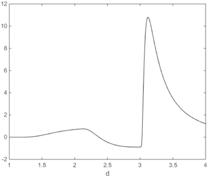
Figure 16. The gradient of antiauxin density, $1\leq d\leq 4$

So how does this connect with Gomez-Campo’s correlation data (Figure 15)? Recalling that positive antiauxin gradient leads to negative correlation of handedness, we reflect Figure 16 about the $x$-axis (multiply $y$-values by $-1$). We could call the resulting $y$-values ”auxin gradient”. Because of the relatively close proximity of the $3^{rd}$ primordium (the angle is $36^{\circ}$ compared to $132^{\circ}$ for the $1^{st}$ and $96^{\circ}$ for the second), the contribution of the $3^{rd}$ primordium (after a short time) is relatively large. At this point all we can say for sure about the relationship between auxin gradient and correlation is that $0$ gradient should give $0$ correlation and the larger the gradient, the larger the correlation. However the gradient can take values from $-\infty$ to $\infty$ and correlation is restricted to between $-1$ to $1$. So trimming down the domain of Figure 16 to $1\leq d\leq 3.2$ and the range from $-1$ to $1$ we have Figure 17.

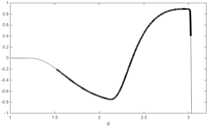
Figure 17. Auxin gradient at a primordium after $d$ plastichrones, $1\leq d\leq 3.2$

The heavy part of the curve was selected so that it goes from the same $y$-value, $-0.2$, that Gomez-Campo’s starts with, to the same $y$-value, $0.4$, that Gomez-Campo’s ends with. The similarity between the two curves (Figure 15 and the dark part of Figure 17) is, we claim, evidence that auxin dynamics in a stem heavily influences the relative handedness of a branch. The biggest difference is the sharper drop after $d=3$ in Figure 17. This is clearly an artifact of our oversimplified model (its 1-dimensionality). Adding in another dimension (or two) would almost certainly smooth out that sharp downturn. Also, increasing $\sigma$ in the model would increase the angular distance to the $3^{rd}$ primordium and soften that hard turn.

If low values (near $0$, but positive and negative) can influence the handedness of a branch, then high values (as seen for $d>3$ in Figure 16) should essentially determine it). There are plants exhibiting each of the extremes (always concordant or always discordant). How those plants differ physiologically is an interesting question. Another puzzle is why these differences (always concordant or always discordant or varying from discordant to concordant) should be built into the development process? The classical ”explanation” of spiral phyllotaxis and the divergence angle of $137.5^{\circ}$ is that it optimizes leaves’ exposure to sunlight. As the measurements of Arabadopsis thaliana show, some (probably most?) plants do not achieve that ideal divergence angle. Distichous plants are not even close. So are these exceptions subject to other selective pressures which causes them deviate from the ideal? We have noticed that some distichous plants (Bananas, Bird of Paradise) grow in clumps and that the outer stems orient their vertical plane tangentially to the circular mass of stems. This would seem to maximize the exposure of their leaves to the sun. Could there be similar causes for choices of relative chirality?

Obviously, our model of the Gomez-Campo phenomenon is a shot in the dark, but hopefully the beginning of a productive discussion.

6. Conclusions and Comments

6.1. Exceptions?

We believe that our model of morphogenesis based on diffusion-driven auxin implies Hofmeister’s Rule. Though infrequent, there are exceptions to Hofmeister’s Rule in the botanical literature (See [5], p.102). One such is monostichy where all the leaves on a stem are aligned on one side. Corn, with its rows of kernels, might seem to be an exception but closer examination of corn shows that the kernels of one row are offset by half a kernel from the neighboring row. 8-row corn (Golden Bantam) is actually 4-jugate and distichous. If corn is n-jugate and distichous then the number of rows on a cob is even, which is generally true as the authoratative website

http://www.agry.purdue.edu/ext/corn/news/timeless/earsize.html

attests. Our guess is that closer inspection of the other apparent exceptions will reveal similar explanations. For instance monostichous plants may have been initiated as distichous but then the primordia on one side not allowed to develop. If this is so, there should be some traces of those primordia that don’t develop (”Ontogeny recapitulates phylogeny”-Ernst Haeckel).

We have had similar experiences several times already. In setting out to examine the implications of diffusion-driven auxin, we initially thought that it would preclude distichous phyllotaxis (as mentioned in Section 2.3) and found to our surprise that distichous phyllotaxy fit right into the model. We had not considered the possibility of random phyllotaxis because it also seemed to violate Hofmeister’s Rule. But since the model allowed it we looked in the literature and there it was: [5], p.102. Most trees, pines, oaks, figs, etc., seem to have random phyllotaxy. In the beginning of our fascination with phyllotaxy we ignored them, saying, ”Plants are like people. Some are better at mathematics than others!” It was a revelation to find that their random phyllotaxy could follow from the same principle as Fibonacci spirals. And the plants with random phyllotaxy may have an important evolutionary advantage. Spiral phyllotaxy can be traced back at least to ancient seas with brown algae. Grasses (with distichous phyllotaxy) were the first plants to grow on land. Trees are a relatively recent development. They evidently compete in crowded environments by randomly sending out branches and then withdrawing nourishment from those that are not productive (of energy from the sun). The ”better mathematicians” don’t seem to have that same ability to adapt to their circumstances.

Green, Steele & Rennich ([4], Chapter 15) considered mechanical buckling of the tunica as an alternative to chemical dynamics (such as our diffusion driven auxin) in explaining phyllotactic patterns. Among the successes they claim is the representation of organs ”in line” ([4], p. 381, Fig. 6A-B). They go on to say, ”Interestingly, the natural, ’in line’ production of organs, seen rarely in flower development (Sattler, 1973; Lacroix and Sattler, 1988), has been presented as special challenge to modelers of phyllotaxis”. It is a special challenge exactly because it contradicts Hofmeister’s rule and is not possible with our model of auxin dynamics. However, flowers have clearly been subjected to more selection pressure than other parts of plants, so one would expect their development to be more complex. This needs further study.

6.2. Distichous to Spiral?

In Section 1.2.1 we modeled distichous phyllotaxis with $\sigma=1/2$ and later argued that any value of $\sigma>\sigma_{0}=\allowbreak 0.374$ would produce distichous phyllotaxis and any value of $\sigma<\sigma_{0}$ would produce spiral phyllotaxis. However, when we ran the calculation for $\sigma=.35$ it was distichous for the first 15 primordia and then transitioned into spiral over the next 5 primordia with a limiting divergence of 153^∘. Clearly the transition from distichous to spiral is more complex than represented in Section 1.2.1. We think what happened at $\sigma=.35$ was that the small bump visible in the graph of Figure 5, though inconseqential by itself, added up over the generations of primordia to something not inconsequential. The closer one gets to the transitional value $\sigma_{0}=\allowbreak 0.374$, the longer the transition from distichous (divergence angle of 180^∘) to spiral takes. For $\sigma=.36$ it only begins at the 50^th primordium and requires about 15 more plastochrones to complete. We have observed that gladiolas exhibit a slow transition from distichous to spiral, ending up with large divergence angles. It could be interesting to study such plants to see if there is a consistent connection between their limit divergence angles and speed of convergence to it.

6.3. Does Nature Favor Concordance or Discordance?

A casual examination of the data gathered by Gomez-Campo for Hirschfeldia incana shows that over the year more branches are discordant than concordant. The average corellation is $-0.055$. The average of all the average corellations for the 6 plants studied by Gomez-Campo is $-.105$. This suggests that the delay, $d$, between the initiation of a primordium and the initiation of its axillary branch for these plants is mostly between $1.5$ and $2.25$ plastichrones, when the influence of the immediate successor dominates. This tendency toward discordance was a surprise since the stability of handedness in a stem is so universal and our examination of bottlebrush had shown a corellation of about $1/3$.

6.4. Possibilities

We believe we have found a window through which the inner workings of plant stems may be viewed. The possibilities for refinement and variation of our model of the Gomez-Campo data are manifest and manifold. Here are a few:

1. Determine the actual limit divergence angle for Hirschfeldia incana (equivalent to determining the corresponding value of $\sigma$. See Figure 13). Then redo the calculation of Section 5.1 with those values. Hopefully, the resulting curve will be a better fit for that of Figure 15.

2. If we begin with small values of $k$ (the ordinal of the $k^{th}$ primordia, $P_{k}$) the alternation of initial divergence angles that showed up in our calculations of Section 2.4.2 and in the table of Section 3.1 should also effect the derivative of the gradient as a function of delay, $d$. Gomez-Campo’s corellation data for Hirschfeldia incana (Figure 15) only has values for $k=2,5,8,11,14,17,20,23,26\&29$ so those alternations, if they exist, have been averaged out. More and better data is called for.

3. The Gomez-Campo data was soley from plants for which branching was a natural part of development. Cutting off the SAM of a stem can force branches (called adventitious branches) to grow, even on stems that normally would not branch. Presumably this happens because a major sink of auxin has been removed. Does the timing and placement of such surgery effect the corellation of chiralities? Recently we examined some stem-branch pairs in xylosma senticosa, a decorative shrub on the UCR campus which is heavily trimmed. Out of a dozen adventitious branches, all were discordant. Can our model shed any light on that?

4. As we noted in Section 3.1(5), the SGRMKP (computer based) model of phyllotaxis does not seem to capture the alternation of divergence angles or their convergence as $k$ becomes large. Is it possible to hybridize SGRMKP model with ours and improve both?

5. The data from measurements on real plants has a stochastic component, probably inherited from the underlying processes such as diffusion. However, our model, based on the mathematics of diffusion, is deterministic. Could incorporation of stochastic processes into our model make it more accurate? For instance, rather than placing the next primordium at the minimum of the antiauxin density, we might distribute it according to a distribution whose density is a monotone function of the antiauxin density. So the lower the antiauxin density, the greater the probability of the primordium being initiated at that point. But what distribution would make the output a better match for reality? Also, it seems reasonable that the distribution should arise from the process for initiating a primordium.

6.5. In Summation

The thing that seems most impressive about our oversimplified model is that it accounts for so many mysterious characteristics of plant stem morphogenesis with just one parameter, $\sigma$. In the model, variations of that one parameter account for the magnitude of divergence angles, their oscillations and limiting values and may well account for different corellations between the handedness of a stem and its branches. $\sigma$ itself is not so readily observable but the other parameters are. If they really do depend on $\sigma$, there should be nonobvious relationships between them which can be verified (or falsified) by direct measurements. If the model passes such tests, then lab experiments to directly verify the role of auxin density could be undertaken, opening up the prospect of guiding plant stem morphogenesis.

7. Appendix

If $X$ is a normal (Gaussian) random variable of mean $0$ and standard deviation $\sigma$, then the mean of the absolute value of $X$ is

$$E\left(\left|X\right|\right) =\frac{1}{\sqrt{2\pi}\sigma}{\displaystyle\int\limits_{-\infty}^{\infty}}\left|x\right|e^{-x^{2}/2\sigma^{2}}dx$$

$$=\frac{1}{\sqrt{2\pi}\sigma}2{\displaystyle\int\limits_{0}^{\infty}}xe^{-x^{2}/2\sigma^{2}}dx$$

$$=\sqrt{\frac{2}{\pi}}{\displaystyle\int\limits_{0}^{\infty}}ue^{-u^{2}/2}\sigma du\text{ if }x=\sigma u$$

$$=\sqrt{\frac{2}{\pi}}\sigma{\displaystyle\int\limits_{0}^{\infty}}ue^{-u^{2}/2}du$$

$$=\sqrt{\frac{2}{\pi}}\sigma{\displaystyle\int\limits_{0}^{\infty}}e^{-z}dz\text{ if }u^{2}/2=z$$

$$=\sqrt{\frac{2}{\pi}}\sigma\left[-e^{-z}|_{0}^{\infty}\right]$$

$$=\sqrt{\frac{2}{\pi}}\sigma\left[-\left(0-1\right)\right]$$

$$=\sqrt{\frac{2}{\pi}}\sigma\text{.}$$

So

$$\sigma=\sqrt{\frac{\pi}{2}}E\left(\left|X\right|\right).$$

Also, the variance of the absolute value of $X$ is

$$Var\left(\left|X\right|\right) =E\left(\left(\left|X\right|-E\left(\left|X\right|\right)\right)^{2}\right)$$

$$=E\left(\left|X\right|^{2}\right)-E^{2}\left(\left|X\right|\right)$$

$$=E\left(X^{2}\right)-E^{2}\left(\left|X\right|\right)$$

$$=\sigma^{2}-\left(\sqrt{\frac{2}{\pi}}\sigma\right)^{2}$$

$$\left(1-\frac{2}{\pi}\right)\sigma^{2}\text{.}$$

So

$$\sigma=\frac{\sqrt{Var\left(\left|X\right|\right)}}{\sqrt{1-\frac{2}{\pi}}}\text{.}$$

References

- [1] Davis, T. Anthony & Davis, B.; Association of coconut foliar spirality with latitude. Mathematical Modeling (Proc. 1st Int. Symp. on Phyllotaxis, Berkeley, July, 1985) (1987), pp. 730-733).
- [2] Gomez-Campo, Cesar; The direction of the phyllotactic helix in axillary shoots of six plant species. Botanical Gazette (1970), pp 110-115.
- [3] Jean, Roger V.; Phyllotaxis: A systematic study of plant morphogenesis, Cambridge U. Press (1994), xiii + 386 pp., ISBN 0-521-40482-7.
- [4] Jean, Roger V. & Barabé, Denis; Symmetry in Plants, World Scientific (1998), pp. li + 835, ISBN 981-02-2621-7.
- [5] Rutishauser, R & Peisl, P.; Phyllotaxy, Handbood of Plant Science, Keith Roberts (Editor), John Wiley & Sons, (2007), pp. 98-103, ISBN 978-0-470-05723(HB).
- [6] Young, David A.; Some thoughts on phyllotaxis, Mathematical Modeling (1987), p. 729.
- [7] Smith, RS; Guyomarc’h; S, Mandel, T; Reinhardt, D; Kuhlemeier, C; Prusinkiewicz, P; A plausible model of phyllotaxis, Proceedings of the National Academy of Sciences USA (PNAS) (2006), pp. 1301-1306.
- [8] Turing, A.; The chemical basis of morphogenesis, Phil. Trans. B (1952), pp. 37-72.