Abstract

The complete set of relations, which mutually express the spacelike and timelike kernel functions for the hadronic vacuum polarization contribution to the muon anomalous magnetic moment $a^{\text{HVP}}_{\mu}$ in terms of each other, is obtained. By making use of the derived relations the explicit expression for the next–to–leading order spacelike kernel function, which enters the representation for $a^{\text{HVP}}_{\mu}$ involving the hadronic vacuum polarization function, is obtained. The corresponding next–to–leading order spacelike kernel function, which appears in the representation for $a^{\text{HVP}}_{\mu}$ involving the Adler function, is calculated numerically. The obtained results can be employed in the assessments of the hadronic vacuum polarization contribution to the muon anomalous magnetic moment in the framework of the spacelike methods, such as lattice studies, MUonE project, and others. Keywords:  muon anomalous magnetic moment, hadronic vacuum polarization contributions, kernel functions, lattice QCD

1 Introduction

The hadronic contribution to the muon anomalous magnetic moment $a_{\mu}=(g_{\mu}-2)/2$ represents one of the long–standing challenging issues of elementary particle physics, which engages the entire pattern of interactions within the Standard Model. The experimental measurements [1, 2] and theoretical evaluations (see a recent comprehensive review [3], which is mainly based on Refs. [4, 5, 6, 7, 8, 9, 10, 11, 12, 13, 14, 15, 16, 17, 18, 19, 20, 21, 22, 23, 24, 25, 26, 27, 28, 29, 30, 31, 32, 33, 34, 35, 36, 37, 38, 39]) of this quantity have achieved an impressive accuracy, and the remaining discrepancy of the order of a few standard deviations between them may be an evidence for the existence of a new fundamental physics beyond the Standard Model. The uncertainty of theoretical estimation of $a_{\mu}$ is largely dominated by the hadronic contribution, which involves the tangled dynamics of colored fields in the infrared domain inaccessible within perturbation theory.

There are basically two approaches to the theoretical assessment of the hadronic vacuum polarization contributions to the muon anomalous magnetic moment $a^{\text{HVP}}_{\mu}$. Specifically, in the framework of the first (“spacelike”) approach $a^{\text{HVP}}_{\mu}$ is commonly represented as the integral of the hadronic vacuum polarization function $\bar{\Pi}(Q^{2})$ [or the related Adler function $D(Q^{2})$] with corresponding kernel functions $K_{\Pi}(Q^{2})$ [or $K_{D}(Q^{2})$] over the entire kinematic interval. Here the perturbative results for the involved functions $\bar{\Pi}(Q^{2})$ and $D(Q^{2})$ have to be supplemented with the relevant nonperturbative inputs. The latter can be provided by, e.g., lattice simulations [40, 41, 42] (which, being capable of delivering valuable insights into the underlying mechanisms, have a large scientific potential), highly anticipated MUonE measurements [43, 44, 45], and other methods. Alternatively, in the framework of the second (“timelike”) approach $a^{\text{HVP}}_{\mu}$ can also be represented as the integral of the function $R(s)$ with respective kernel functions $K_{R}(s)$. Here the perturbative results for the function $R(s)$ are usually complemented by the low–energy experimental data on the $R$–ratio of electron–positron annihilation into hadrons, that constitutes the data–driven method of evaluation of $a^{\text{HVP}}_{\mu}$. In turn, the “spacelike” and “timelike” kernel functions can be calculated within various techniques, such as the mass operator approach [46, 47, 48], the hyperspherical approach [49, 50, 51, 52], the dispersive method [53, 54, 55, 56, 57], and the asymptotic expansion method [58, 59, 11]. The “timelike” kernel functions have been extensively studied over the past decades, whereas the corresponding “spacelike” kernel functions remain largely unavailable.

The primary objective of this paper is to derive the complete set of relations, which mutually express the “spacelike” and “timelike” kernel functions $K_{\Pi}(Q^{2})$, $K_{D}(Q^{2})$, and $K_{R}(s)$ in terms of each other, and to calculate the explicit expression for the next–to–leading order “spacelike” kernel function $K_{\Pi}^{(3a)}(Q^{2})$ by making use of the obtained relations.

The layout of the paper is as follows. Section 2 recaps the essentials of the dispersion relations for the hadronic vacuum polarization function $\bar{\Pi}(Q^{2})$, the Adler function $D(Q^{2})$, and the function $R(s)$, and expounds the basics of the hadronic vacuum polarization contributions to the muon anomalous magnetic moment. In Sect. 3 the complete set of relations, which mutually express the kernel functions $K_{\Pi}(Q^{2})$, $K_{D}(Q^{2})$, and $K_{R}(s)$ in terms of each other, is obtained, and the explicit expression for the “spacelike” kernel function $K_{\Pi}^{(3a)}(Q^{2})$ is calculated. Section 4 summarizes the basic results. The “timelike” kernel function $K_{R}^{(3a)}(s)$ is given in the App. A.

2 Methods

2.1 General dispersion relations

Let us begin by briefly elucidating the essentials of dispersion relations for the hadronic vacuum polarization function $\Pi(q^{2})$, the Adler function $D(Q^{2})$, and the function $R(s)$ (the detailed description of this issue can be found in, e.g., Chap. 1 of Ref. [60] and references therein). The theoretical exploration of a certain class of the strong interaction processes is primarily based on the hadronic vacuum polarization function $\Pi(q^{2})$, which is defined as the scalar part of the hadronic vacuum polarization tensor

$$\Pi_{\mu\nu}(q^{2})=i\!\int\!d^{4}x\,e^{iqx}\bigl{\langle}0\bigl{|}\,T\!\left\{J_{\mu}(x)\,J_{\nu}(0)\right\}\bigr{|}0\bigr{\rangle}=\frac{i}{12\pi^{2}}(q_{\mu}q_{\nu}-g_{\mu\nu}q^{2})\Pi(q^{2}).$$ (1)

As discussed in, e.g., Ref. [61], the function $\Pi(q^{2})$ (1) has the only cut along the positive semiaxis of real $q^{2}$ starting at the hadronic production threshold $q^{2}\geq s_{0}$, that leads to

$$\Delta\Pi(q^{2},q_{0}^{2})=(q^{2}-q_{0}^{2})\int\limits_{s_{0}}^{\infty}\frac{R(\sigma)}{(\sigma-q^{2})(\sigma-q_{0}^{2})}\,d\sigma,$$ (2)

where

$$\Delta\Pi(q^{2},q_{0}^{2})=\Pi(q^{2})-\Pi(q_{0}^{2}),\qquad\Pi(0)=0,\qquad\Delta\Pi(0,-p^{2})=-\Pi(-p^{2})=\bar{\Pi}(p^{2}),$$ (3)

and

$$R(s)=\frac{1}{2\pi i}\lim_{\varepsilon\to 0_{+}}\Bigl{[}\Pi(s+i\varepsilon)-\Pi(s-i\varepsilon)\Bigr{]}.$$ (4)

The function $R(s)$ (4) is commonly identified with the so–called $R$–ratio of electron–positron annihilation into hadrons

$$R(s)=\frac{\sigma(e^{+}e^{-}\to\text{hadrons};s)}{\sigma(e^{+}e^{-}\to\mu^{+}\mu^{-};s)}\,,$$ (5)

where $s=q^{2}>0$ is the timelike kinematic variable, namely, the center–of–mass energy squared. At the same time, in practical applications it proves to be convenient to deal with the Adler function [62]

$$D(Q^{2})=-\,\frac{d\,\Pi(-Q^{2})}{d\ln Q^{2}},$$ (6)

where $Q^{2}=-q^{2}>0$ stands for the spacelike kinematic variable. The corresponding dispersion relation [62]

$$D(Q^{2})=Q^{2}\int\limits_{s_{0}}^{\infty}\frac{R(\sigma)}{(\sigma+Q^{2})^{2}}\,d\sigma$$ (7)

immediately follows from Eqs. (2) and (6).

2.2 Hadronic vacuum polarization contributions to $a_{\mu}$

In the framework of the “timelike” (or data–driven) method of assessment of the hadronic vacuum polarization contributions to the muon anomalous magnetic moment the latter is commonly represented in terms of the $R$–ratio of electron–positron annihilation into hadrons (4). In the leading order of perturbation theory (namely, in the second order in the electromagnetic coupling) the corresponding contribution is given by the diagram displayed in Fig. 1, that yields [63, 64, 65]

$$a^{\text{HVP}(2)}_{\mu}=\frac{1}{3}\Bigl{(}\frac{\alpha}{\pi}\Bigr{)}^{\!2}\!\int\limits_{s_{0}}^{\infty}\frac{G_{2}(s)}{s}R(s)ds,$$ (8)

where

$$G_{2}(s)=\int\limits_{0}^{1}\!\frac{x^{2}(1-x)}{x^{2}+(1-x)s/m_{\mu}^{2}}\,dx$$ (9)

and $s=q^{2}\geq 0$ denotes the timelike kinematic variable. The kernel function $G_{2}(s)$ (9) can also be represented in explicit form [63, 66, 67, 68] and the expression appropriate for the practical applications reads

$$G_{2}(s)=\frac{1}{2}+4\eta\Bigl{[}(2\eta-1)\ln(4\eta)-1\Bigr{]}-2\Bigl{[}2(2\eta-1)^{2}-1\Bigr{]}\frac{A(\eta)}{\psi(\eta)},$$ (10)

where

$$\psi(\eta)=\frac{\sqrt{\eta-1}}{\sqrt{\eta}},\qquad A(\eta)={\rm arctanh}\Bigl{[}\psi(\eta)\Bigr{]},\qquad\eta=\frac{s}{4m_{\mu}^{2}}.$$ (11)

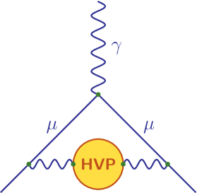
Figure 1: The leading–order hadronic vacuum polarization contribution to the muon anomalous magnetic moment (8).

Factually, the specific form of the kernel function $G_{2}(s)$ (9) makes it possible to express the leading–order contribution (8) in terms of the “spacelike” hadronic vacuum polarization function $\bar{\Pi}(Q^{2})$ [Eqs. (2), (3)] and the Adler function $D(Q^{2})$ (6), but only in this particular case (a discussion of this issue can be found in, e.g., Ref. [69]). Namely, Eqs. (8), (9), (2), and (3) can be reduced to [70]

$$a^{\text{HVP}(2)}_{\mu} =\frac{1}{3}\Bigl{(}\frac{\alpha}{\pi}\Bigr{)}^{\!2}\!\int\limits_{0}^{1}\!dx(1-x)\!\!\int\limits_{s_{0}}^{\infty}\!\frac{ds}{s}\frac{m_{\mu}^{2}x^{2}(1-x)^{-1}}{s+m_{\mu}^{2}x^{2}(1-x)^{-1}}R(s)=$$

$$=\frac{1}{3}\Bigl{(}\frac{\alpha}{\pi}\Bigr{)}^{\!2}\!\int\limits_{0}^{1}\!(1-x)\bar{\Pi}\biggl{(}\!m_{\mu}^{2}\frac{x^{2}}{1-x}\biggr{)}dx,$$ (12)

where $\bar{\Pi}(Q^{2})=\Delta\Pi(0,-Q^{2})$ and $Q^{2}=-q^{2}\geq 0$ stands for the spacelike kinematic variable. In turn, Eq. (2.2) can also be represented in terms of the Adler function (6) by making use of the integration by parts, that eventually yields [71, 69]

$$a^{\text{HVP}(2)}_{\mu}=\frac{1}{3}\Bigl{(}\frac{\alpha}{\pi}\Bigr{)}^{\!2}\!\int\limits_{0}^{1}\!(1-x)\biggl{(}\!1-\frac{x}{2}\biggr{)}D\biggl{(}\!m_{\mu}^{2}\frac{x^{2}}{1-x}\biggr{)}\frac{dx}{x}.$$ (13)

It is necessary to emphasize here that this way of the derivation of the “spacelike” expressions (2.2) and (13) from the “timelike” one (8) entirely relies on the particular form of the leading–order kernel function $G_{2}(s)$ (9) and cannot be performed in any other case.

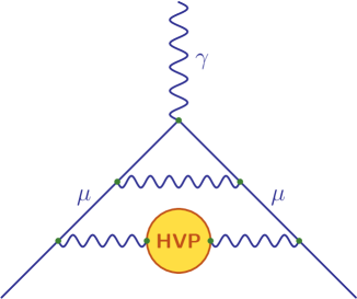
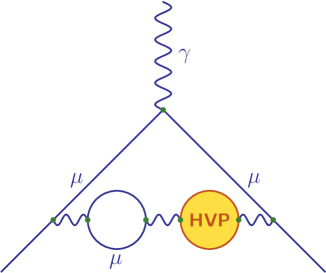
Figure 2: Two of the diagrams contributing to $a^{\text{HVP}(3a)}_{\mu}$ (14).

In the next–to–leading order of perturbation theory (namely, in the third order in the electromagnetic coupling) the hadronic vacuum polarization contribution to the muon anomalous magnetic moment $a^{\text{HVP}(3)}_{\mu}$ is composed of three parts. Specifically, the first part $a^{\text{HVP}(3a)}_{\mu}$ corresponds to the diagrams, which include (in addition to the hadronic insertion shown in Fig. 1) one photon line or closed muon loop, see Fig. 2. In turn, the second part $a^{\text{HVP}(3b)}_{\mu}$ corresponds to the diagrams, which additionally include one closed electron (or $\tau$–lepton) loop, whereas the third part $a^{\text{HVP}(3c)}_{\mu}$ corresponds to the diagram with double hadronic insertion. In what follows we shall primarily focus on the first part of $a^{\text{HVP}(3)}_{\mu}$, which can be represented as

$$a^{\text{HVP}(3a)}_{\mu}=\frac{2}{3}\Bigl{(}\frac{\alpha}{\pi}\Bigr{)}^{\!3}\!\int\limits_{s_{0}}^{\infty}\frac{G_{3a}(s)}{s}R(s)ds.$$ (14)

The “timelike” kernel function $G_{3a}(s)$ entering this equation has been calculated explicitly in Ref. [57], see App. A. However, the explicit form of the corresponding kernel functions required for the assessment of $a^{\text{HVP}(3a)}_{\mu}$ within “spacelike” methods is still unavailable.

3 Results and discussion

3.1 Relations between the kernel functions

First of all, for practical purposes it is convenient to represent the hadronic vacuum polarization contribution to the muon anomalous magnetic moment, which corresponds to the $\ell$–th order in the electromagnetic coupling, in the following form

$$a^{\text{HVP}(\ell)}_{\mu} =A_{0}^{(\ell)}\!\!\int\limits_{0}^{\infty}\!K_{\Pi}^{(\ell)}(Q^{2})\bar{\Pi}(Q^{2})\frac{dQ^{2}}{4m_{\mu}^{2}}=A_{0}^{(\ell)}\!\!\int\limits_{0}^{\infty}\!\tilde{K}_{\Pi}^{(\ell)}(\zeta)\bar{\Pi}(4\zeta m_{\mu}^{2})d\zeta=$$ (15a)

$$=A_{0}^{(\ell)}\!\!\int\limits_{0}^{\infty}\!K_{D}^{(\ell)}(Q^{2})D(Q^{2})\frac{dQ^{2}}{4m_{\mu}^{2}}=A_{0}^{(\ell)}\!\!\int\limits_{0}^{\infty}\!\tilde{K}_{D}^{(\ell)}(\zeta)D(4\zeta m_{\mu}^{2})d\zeta=$$ (15b)

$$=A_{0}^{(\ell)}\!\!\int\limits_{s_{0}}^{\infty}\!K_{R}^{(\ell)}(s)R(s)\frac{ds}{4m_{\mu}^{2}}=A_{0}^{(\ell)}\!\!\int\limits_{\chi}^{\infty}\!\tilde{K}_{R}^{(\ell)}(\eta)R(4\eta m_{\mu}^{2})d\eta.$$ (15c)

In this equation $A_{0}^{(\ell)}$ is a constant prefactor, $\bar{\Pi}(Q^{2})=\Delta\Pi(0,-Q^{2})$ is defined in Eq. (3), $Q^{2}=-q^{2}\geq 0$ and $s=q^{2}\geq 0$ stand, respectively, for the spacelike and timelike kinematic variables, $\zeta=Q^{2}/(4m_{\mu}^{2})$ and $\eta=s/(4m_{\mu}^{2})$ denote the dimensionless kinematic variables, and $\chi=s_{0}/(4m_{\mu}^{2})$. For example, for the leading–order hadronic vacuum polarization contribution (8)

$$A_{0}^{(2)}=\frac{1}{3}\Bigl{(}\frac{\alpha}{\pi}\Bigr{)}^{\!2},\qquad\tilde{K}_{R}^{(2)}(\eta)=K_{R}^{(2)}(4\eta m_{\mu}^{2})=G_{2}(4\eta m_{\mu}^{2})\frac{1}{\eta}.$$ (16)

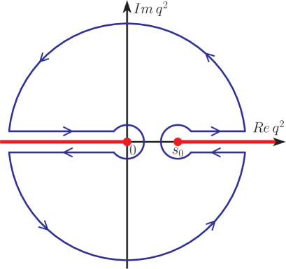
Figure 3: The closed integration contour $C$ in the complex $q^{2}$–plane in Eq. (17). The physical cut $q^{2}\geq s_{0}$ of the hadronic vacuum polarization function $\Pi(q^{2})=-\bar{\Pi}(-q^{2})$ (3) is shown along the positive semiaxis of real $q^{2}$, whereas the physical cut $q^{2}\leq 0$ of the “timelike” kernel function $K_{R}(q^{2})$ (15c) is shown along the negative semiaxis of real $q^{2}$.

In fact, the kernel functions $K_{\Pi}(Q^{2})$, $K_{D}(Q^{2})$, and $K_{R}(s)$ appearing in Eq. (15) can all be expressed in terms of each other. Let us begin by expressing the “spacelike” kernel function $K_{\Pi}(Q^{2})$ (15a) in terms of the “timelike” one $K_{R}(s)$ (15c). As mentioned earlier, the hadronic vacuum polarization function $\Pi(q^{2})=-\bar{\Pi}(-q^{2})$ (3) possesses the only cut along the positive semiaxis of real $q^{2}$ starting at the hadronic production threshold $q^{2}\geq s_{0}$, whereas the kernel function $K_{R}(q^{2})$ (15c) has the only cut along the negative semiaxis of real $q^{2}$ starting at the origin $q^{2}\leq 0$, see, e.g., Ref. [57]. Therefore, the integral of the product of the functions $K_{R}(q^{2})$ (15c) and $\bar{\Pi}(-q^{2})$ (3) along the contour displayed in Fig. 3 vanishes, namely

$$\oint_{C}K_{R}(q^{2})\bar{\Pi}(-q^{2})dq^{2}=0,$$ (17)

that can also be represented as

$$\int\limits_{\infty-i\varepsilon}^{s_{0}-i\varepsilon}K_{R}(q^{2})\bar{\Pi}(-q^{2})dq^{2}+\int\limits_{s_{0}+i\varepsilon}^{\infty+i\varepsilon}K_{R}(q^{2})\bar{\Pi}(-q^{2})dq^{2}+$$

$$+\int\limits_{-\infty+i\varepsilon}^{i\varepsilon}K_{R}(q^{2})\bar{\Pi}(-q^{2})dq^{2}+\int\limits_{-i\varepsilon}^{-\infty-i\varepsilon}K_{R}(q^{2})\bar{\Pi}(-q^{2})dq^{2}=0.$$ (18)

The change of the integration variables $q^{2}=p^{2}-i\varepsilon$ in the first and fourth terms of Eq. (3.1) and $q^{2}=p^{2}+i\varepsilon$ in its second and third terms casts Eq. (3.1) to

$$-\frac{1}{2\pi i}\lim_{\varepsilon\to 0_{+}}\int\limits_{0}^{-\infty}\bar{\Pi}(-p^{2})\Bigl{[}K_{R}(p^{2}+i\varepsilon)-K_{R}(p^{2}-i\varepsilon)\Bigr{]}dp^{2}=\int\limits_{s_{0}}^{\infty}K_{R}(p^{2})R(p^{2})dp^{2},$$ (19)

where the limit $\varepsilon\to 0_{+}$ is assumed and Eq. (4) is employed. Then the change of the integration variables $p^{2}=-Q^{2}$ on the left–hand side of Eq. (19) and $p^{2}=s$ on its right–hand side leads to

$$\int\limits_{0}^{\infty}\bar{\Pi}(Q^{2})K_{\Pi}(Q^{2})dQ^{2}=\int\limits_{s_{0}}^{\infty}K_{R}(s)R(s)ds,$$ (20)

where

$$K_{\Pi}(Q^{2})=\frac{1}{2\pi i}\lim_{\varepsilon\to 0_{+}}\Bigl{[}K_{R}(-Q^{2}+i\varepsilon)-K_{R}(-Q^{2}-i\varepsilon)\Bigr{]},\qquad Q^{2}\geq 0.$$ (21)

This relation has also been independently derived in a different way in Ref. [72].

In turn, the relation inverse to Eq. (21) directly follows from Eqs. (15a) and (2), specifically

$$\int\limits_{0}^{\infty}K_{\Pi}(Q^{2})\bar{\Pi}(Q^{2})\frac{dQ^{2}}{4m_{\mu}^{2}}=\int\limits_{0}^{\infty}\frac{dQ^{2}}{4m_{\mu}^{2}}K_{\Pi}(Q^{2})\,Q^{2}\!\!\int\limits_{s_{0}}^{\infty}\frac{ds}{s}\,\frac{R(s)}{s+Q^{2}}=\int\limits_{s_{0}}^{\infty}K_{R}(s)R(s)\frac{ds}{4m_{\mu}^{2}},$$ (22)

where

$$K_{R}(s)=\frac{1}{s}\int\limits_{0}^{\infty}K_{\Pi}(Q^{2})\frac{Q^{2}}{s+Q^{2}}\,dQ^{2},\qquad s\geq 0.$$ (23)

The “timelike” kernel function $K_{R}(s)$ (15c) can be expressed in terms of the “spacelike” one $K_{D}(Q^{2})$ (15b) in a similar way. In particular, Eqs. (15b) and (7) imply

$$\int\limits_{0}^{\infty}K_{D}(Q^{2})D(Q^{2})\frac{dQ^{2}}{4m_{\mu}^{2}}=\int\limits_{0}^{\infty}\frac{dQ^{2}}{4m_{\mu}^{2}}K_{D}(Q^{2})\,Q^{2}\!\!\int\limits_{s_{0}}^{\infty}\frac{R(s)}{(s+Q^{2})^{2}}\,ds=\int\limits_{s_{0}}^{\infty}K_{R}(s)R(s)\frac{ds}{4m_{\mu}^{2}},$$ (24)

where

$$K_{R}(s)=\int\limits_{0}^{\infty}K_{D}(Q^{2})\frac{Q^{2}}{(s+Q^{2})^{2}}\,dQ^{2},\qquad s\geq 0.$$ (25)

In turn, the corresponding relation between the kernel functions $K_{\Pi}(Q^{2})$ (15a) and $K_{D}(Q^{2})$ (15b) can be derived from Eqs. (6) and (15b), namely

$$\int\limits_{0}^{\infty}K_{D}(Q^{2})D(Q^{2})dQ^{2}=-\int\limits_{0}^{\infty}dQ^{2}K_{D}(Q^{2})\,Q^{2}\,\frac{d\,\Pi(-Q^{2})}{d\,Q^{2}}=$$

$$=K_{D}(Q^{2})\,Q^{2}\,\bar{\Pi}(Q^{2})\Biggr{|}_{0}^{\infty}-\int\limits_{0}^{\infty}\bar{\Pi}(Q^{2})\biggl{[}K_{D}(Q^{2})+\frac{d\,K_{D}(Q^{2})}{d\,\ln Q^{2}}\biggr{]}dQ^{2},$$ (26)

with the integration by parts being used. Since the first term of this equation vanishes (see also remarks given below), Eqs. (15a) and (3.1) yield

$$K_{\Pi}(Q^{2})=-\biggl{[}K_{D}(Q^{2})+\frac{d\,K_{D}(Q^{2})}{d\,\ln Q^{2}}\biggr{]},\qquad Q^{2}\geq 0.$$ (27)

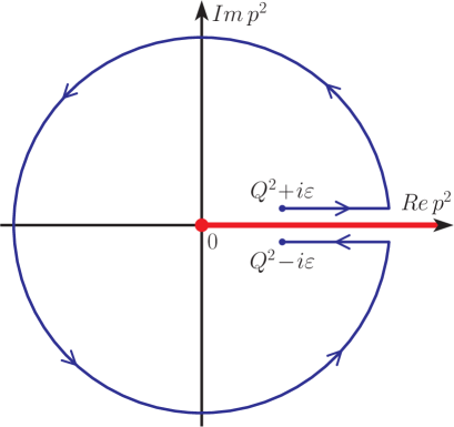
Figure 4: The integration contour in the complex $p^{2}$–plane in Eq. (33). The physical cut $p^{2}\geq 0$ of the “timelike” kernel function $K_{R}(-p^{2})$ (15c) is shown along the positive semiaxis of real $p^{2}$.

The kernel function $K_{D}(Q^{2})$ (15b) can be expressed in terms of $K_{\Pi}(Q^{2})$ (15a) in the following way. The solution to the differential equation (27)

$$K_{D}(Q^{2})+\frac{d\,K_{D}(Q^{2})}{d\,\ln Q^{2}}=-K_{\Pi}(Q^{2})$$ (28)

reads

$$K_{D}(Q^{2})=\frac{1}{Q^{2}}\biggl{[}-\!\int\!\!K_{\Pi}(Q^{2})\,dQ^{2}+c_{0}\biggr{]}\!,$$ (29)

where $c_{0}$ denotes an arbitrary integration constant. The latter has to be chosen in the way that prevents the appearance of the mutually canceling divergences at the upper limit of both terms in the second line of Eq. (3.1). Specifically, the integration constant $c_{0}$ has to subtract the value of the antiderivative of the function $K_{\Pi}(Q^{2})$ at $Q^{2}\to\infty$, that eventually results in

$$K_{D}(Q^{2})=\frac{1}{Q^{2}}\int\limits_{Q^{2}}^{\infty}\!\!K_{\Pi}(\xi)\,d\xi,\qquad\xi=-p^{2}\geq 0,$$ (30)

where $\xi$ stands for a spacelike kinematic variable. It is worthwhile to note also that Eqs. (30) and (23) imply that the functions $Q^{2}K_{D}(Q^{2})$ and $sK_{R}(s)$ acquire the same value in the infrared limit, namely

$$\lim_{Q^{2}\to 0_{+}}Q^{2}K_{D}(Q^{2})=\lim_{s\to 0_{+}}sK_{R}(s)=\int\limits_{0}^{\infty}\!\!K_{\Pi}(\xi)\,d\xi.$$ (31)

Finally, the relation inverse to Eq. (25) can be derived by making use of Eqs. (30) and (21), namely

$$K_{D}(Q^{2})=-\frac{1}{2\pi i}\lim_{\varepsilon\to 0_{+}}\frac{1}{Q^{2}}\int\limits_{Q^{2}}^{\infty}\Bigl{[}K_{R}(-\xi-i\varepsilon)-K_{R}(-\xi+i\varepsilon)\Bigr{]}d\xi.$$ (32)

The change of the integration variables $\xi=p^{2}-i\varepsilon$ and $\xi=p^{2}+i\varepsilon$ in, respectively, the first and the second terms in the square brackets in Eq. (32) eventually leads to

$$K_{D}(Q^{2})=-\frac{1}{2\pi i}\lim_{\varepsilon\to 0_{+}}\frac{1}{Q^{2}}\int\limits_{Q^{2}+i\varepsilon}^{Q^{2}-i\varepsilon}K_{R}(-p^{2})dp^{2},$$ (33)

where the integration contour on the right–hand side of this equation lies in the region of analyticity of the function $K_{R}(-p^{2})$, see Fig. 4.

Thus, the derived equations (21), (23), (25), (27), (30), and (33) constitute the complete set of relations, which mutually express the “spacelike” and “timelike” kernel functions $K_{\Pi}(Q^{2})$, $K_{D}(Q^{2})$, and $K_{R}(s)$ entering Eq. (15) in terms of each other.

3.2 The “spacelike” kernel functions

The relations obtained in Sect. 3.1 enable one to calculate the unknown kernel functions (15) by making use of the known ones. To exemplify this method, let us first address the hadronic vacuum polarization contribution to the muon anomalous magnetic moment in the leading order.

Specifically, the explicit form of the “spacelike” kernel function $K_{\Pi}^{(2)}(Q^{2})$ (15a) can be obtained directly from the corresponding “timelike” one $K_{R}^{(2)}(s)$ [Eqs. (10), (16)] by making use of the derived relation (21), that eventually results in

$$\zeta\tilde{K}_{\Pi}^{(2)}(\zeta)=\frac{1}{\zeta^{2}}\,\frac{y^{5}(\zeta)}{1-y(\zeta)},\qquad y(\zeta)=\zeta\Bigl{(}\sqrt{1+\zeta^{-1}}-1\Bigr{)},\qquad\zeta=\frac{Q^{2}}{4m_{\mu}^{2}}.$$ (34)

It is worth noting that Eq. (34) is identical to the result of the mapping the integration range $0\leq x<1$ in Eq. (2.2) onto the kinematic interval $0\leq Q^{2}<\infty$ reported in Refs. [73, 74, 69] and to the result of straightforward calculation [75] performed within the technique [49, 50, 51, 52].

In turn, the explicit form of the kernel function $K_{D}^{(2)}(Q^{2})$ (15b) can be derived from Eq. (34) by making use of the obtained relation (30), that leads to

$$\zeta\tilde{K}_{D}^{(2)}(\zeta)=(2\zeta+1)^{2}-2(2\zeta+1)\sqrt{\zeta(\zeta+1)}-\frac{1}{2}.$$ (35)

This equation coincides with the result of the mapping the integration range $0\leq x<1$ in Eq. (13) onto the kinematic interval $0\leq Q^{2}<\infty$, see Refs. [73, 69].

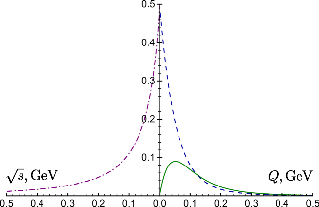
Figure 5: The kernel functions $\zeta\tilde{K}_{\Pi}^{(2)}(\zeta)$ [Eq. (34), solid curve], $\zeta\tilde{K}_{D}^{(2)}(\zeta)$ [Eq. (35), dashed curve], and $\eta\tilde{K}_{R}^{(2)}(\eta)$ [Eqs. (10), (16), dot–dashed curve] in the spacelike [$Q^{2}=-q^{2}\geq 0$, $\zeta=Q^{2}/(4m_{\mu}^{2})$] and timelike [$s=q^{2}\geq 0$, $\eta=s/(4m_{\mu}^{2})$] domains.

The “spacelike” [$K_{\Pi}^{(2)}(Q^{2})$, Eq. (34) and $K_{D}^{(2)}(Q^{2})$, Eq. (35)] and “timelike” [$K_{R}^{(2)}(s)$, Eqs. (10), (16)] kernel functions satisfy all six relations (21), (23), (25), (27), (30), and (33) derived in Sect. 3.1. The plots of the kernel functions (34), (35), and (10) are displayed in Fig. 5. In particular, as one can infer from this figure, in the infrared limit the kernel functions $\zeta\tilde{K}_{D}^{(2)}(\zeta)$ (35) and $\eta\tilde{K}_{R}^{(2)}(\eta)$ (10) assume the same value $1/2$, as determined by the relation (31).

In the next–to–leading order the explicit form of the uncalculated yet “spacelike” kernel function $K_{\Pi}^{(3a)}(Q^{2})$ appearing in Eq. (15a) can be obtained in a similar way. Specifically, the derived relation (21) and Eq. (A) eventually result in

$$\zeta\tilde{K}^{(3a)}_{\text{$\Pi$}}(\zeta) =-\biggl{[}\frac{19}{12}+\frac{7}{9}\zeta+\frac{23}{9}\zeta^{2}-\frac{1}{4(\zeta+1)}\biggr{]}+$$

$$+\biggl{(}\frac{1}{3\zeta}+\frac{127}{36}+\frac{115}{18}\zeta+\frac{23}{9}\zeta^{2}\biggr{)}\psi(\zeta+1)-$$

$$-\frac{5}{3}\zeta^{2}\ln(4\zeta)-\biggl{(}\frac{14}{3}\zeta+1\biggr{)}(\zeta+1)\psi(\zeta+1)\times$$

$$\times\biggl{\{}\frac{1}{2}\ln(4\zeta)+3A(\zeta+1)+2\ln\Bigl{[}1+B(\zeta+1)\Bigr{]}\!\biggr{\}}+$$

$$+\biggl{(}-\frac{19}{6}+\frac{53}{3}\zeta+\frac{58}{3}\zeta^{2}-\frac{1}{3\zeta}+\frac{2}{\zeta+1}\biggr{)}A(\zeta+1)+$$

$$+\biggl{[}\frac{13}{12\,\zeta}+\frac{7}{6}+\zeta+\frac{8}{3}\zeta^{2}+\frac{1}{4\zeta(\zeta+1)}\biggr{]}\psi(\zeta+1)A(\zeta+1)-$$

$$-\biggl{(}\frac{1}{2}+\frac{14}{3}\zeta+8\zeta^{2}\biggr{)}\times$$

$$\times\biggl{\{}2A(\zeta+1)\Bigl{\{}2\ln\bigl{[}1+B(\zeta+1)\bigr{]}+\ln\bigl{[}1-B(\zeta+1)\bigr{]}\!\Bigr{\}}-$$

$$-2\Bigl{\{}{\rm Li}_{2}\bigl{[}B(\zeta+1)\bigr{]}+2{\rm Li}_{2}\bigl{[}-B(\zeta+1)\bigr{]}\!\Bigr{\}}\!\biggr{\}}.$$ (36)

An equivalent form of this equation has been independently derived in Ref. [72]. In Eq. (3.2) $\zeta=Q^{2}/(4m_{\mu}^{2})$, $Q^{2}=-q^{2}\geq 0$ stands for the spacelike kinematic variable, the functions $\psi(\zeta)$ and $A(\zeta)$ are defined in Eq. (11),

$$B(\zeta)=\frac{1-\psi(\zeta)}{1+\psi(\zeta)},$$ (37)

and

$${\rm Li}_{2}(y)=-\int\limits_{0}^{y}\ln(1-t)\frac{d\,t}{t}$$ (38)

denotes the dilogarithm function.

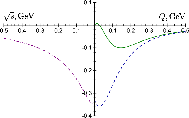
Figure 6: The kernel functions $\zeta\tilde{K}_{\Pi}^{(3a)}(\zeta)$ [Eq. (3.2), solid curve], $\zeta\tilde{K}_{D}^{(3a)}(\zeta)$ [Eqs. (30), (3.2), dashed curve], and $\eta\tilde{K}_{R}^{(3a)}(\eta)$ [Eq. (A), dot–dashed curve] in the spacelike [$Q^{2}=-q^{2}\geq 0$, $\zeta=Q^{2}/(4m_{\mu}^{2})$] and timelike [$s=q^{2}\geq 0$, $\eta=s/(4m_{\mu}^{2})$] domains.

It is straightforward to verify that the “spacelike” [$K_{\Pi}^{(3a)}(Q^{2})$, Eq. (3.2)] and “timelike” [$K_{R}^{(3a)}(s)$, Eq. (A)] kernel functions satisfy the corresponding relations (21) and (23) obtained in Sect. 3.1. The plots of the kernel functions [$K_{\Pi}^{(3a)}(Q^{2})$, Eq. (3.2)], [$K_{D}^{(3a)}(Q^{2})$, computed numerically by making use of Eqs. (30) and (3.2)], and [$K_{R}^{(3a)}(s)$, Eq. (A)] are displayed in Fig. 6. As one can infer from this figure, in the infrared limit the kernel functions $\zeta\tilde{K}_{D}^{(3a)}(\zeta)$ [Eqs. (30), (3.2)] and $\eta\tilde{K}_{R}^{(3a)}(\eta)$ [Eq. (A)] acquire the same value determined by the relation (31), specifically

$$\lim_{\zeta\to 0_{+}}\zeta\tilde{K}_{D}^{(3a)}(\zeta)=\lim_{\eta\to 0_{+}}\eta\tilde{K}_{R}^{(3a)}(\eta)=\frac{197}{144}+\frac{1}{2}\zeta_{2}-3\zeta_{2}\ln(2)+\frac{3}{4}\zeta_{3}\simeq-0.328479,$$ (39)

where

$$\zeta_{t}=\sum_{n=1}^{\infty}\frac{1}{n^{t}}$$ (40)

stands for the Riemann $\zeta$ function.

4 Conclusions

The complete set of relations [Eqs. (21), (23), (25), (27), (30), (33)], which mutually express the “spacelike” [$K_{\Pi}(Q^{2})$, Eq. (15a) and $K_{D}(Q^{2})$, Eq. (15b)] and “timelike” [$K_{R}(s)$, Eq. (15c)] kernel functions in terms of each other, is obtained. By making use of the derived relations the explicit expression for the next–to–leading order “spacelike” kernel function $K_{\Pi}^{(3a)}(Q^{2})$ is calculated [Eq. (3.2)] and the kernel function $K_{D}^{(3a)}(Q^{2})$ is computed numerically [Eqs. (30), (3.2) and Fig. 6]. The obtained results can be employed in the assessments of the hadronic vacuum polarization contributions to the muon anomalous magnetic moment in the framework of the spacelike methods, such as lattice studies [40, 41], MUonE project [43, 44, 45], and others.

Appendix A The “timelike” kernel function $K^{(3a)}_{\text{$R$}}(s)$

As mentioned earlier, the next–to–leading order hadronic vacuum polarization contribution to the muon anomalous magnetic moment (14) can be represented as

$$a^{\text{HVP}(3a)}_{\mu}=A_{0}^{(3a)}\!\!\int\limits_{s_{0}}^{\infty}\!K_{R}^{(3a)}(s)R(s)\frac{ds}{4m_{\mu}^{2}}=A_{0}^{(3a)}\!\!\int\limits_{\chi}^{\infty}\!\tilde{K}_{R}^{(3a)}(\eta)R(4\eta m_{\mu}^{2})d\eta,$$ (41)

where

$$A_{0}^{(3a)}=\frac{2}{3}\Bigl{(}\frac{\alpha}{\pi}\Bigr{)}^{\!3},\quad\tilde{K}_{R}^{(3a)}(\eta)=K_{R}^{(3a)}(4\eta m_{\mu}^{2})=G_{3a}(4\eta m_{\mu}^{2})\frac{1}{\eta},\quad\eta=\frac{s}{4m_{\mu}^{2}},\quad\chi=\frac{s_{0}}{4m_{\mu}^{2}}.$$ (42)

The explicit form of the “timelike” kernel function entering Eq. (41) was calculated in Ref. [57], namely

$$\eta\tilde{K}^{(3a)}_{\text{$R$}}(\eta) =-\frac{139}{144}+\frac{115}{18}\eta+$$

$$+\biggl{[}\frac{19}{12}-\frac{7}{9}\eta+\frac{23}{9}\eta^{2}+\frac{1}{4(\eta-1)}\biggr{]}\ln(4\eta)+$$

$$+\biggl{[}\frac{2}{3\,\eta}-\frac{127}{18}+\frac{115}{9}\eta-\frac{46}{9}\eta^{2}\biggr{]}\frac{1}{\psi(\eta)}A(\eta)+$$

$$+\biggl{(}\frac{9}{4}+\frac{5}{6}\eta-8\eta^{2}-\frac{1}{2\,\eta}\biggr{)}\zeta_{2}+\frac{5}{6}\eta^{2}\ln^{2}(4\eta)+$$

$$+\biggl{(}\frac{14}{3}\eta-1\biggr{)}(\eta-1)\frac{1}{\psi(\eta)}T_{1}(\eta)+$$

$$+\biggl{(}\frac{19}{6}+\frac{53}{3}\eta-\frac{58}{3}\eta^{2}-\frac{1}{3\,\eta}+\frac{2}{\eta-1}\biggr{)}A^{2}(\eta)+$$

$$+\biggl{[}\frac{13}{12\,\eta}-\frac{7}{6}+\eta-\frac{8}{3}\eta^{2}-\frac{1}{4\eta(\eta-1)}\biggr{]}\frac{1}{\psi(\eta)}T_{2}(\eta)+$$

$$+\biggl{(}\frac{1}{2}-\frac{14}{3}\eta+8\eta^{2}\biggl{)}T_{3}(\eta),$$ (43)

where $\eta=s/(4m_{\mu}^{2})$, $s=q^{2}\geq 0$ is the timelike kinematic variable, the functions $\psi(\eta)$, $A(\eta)$, and $B(\eta)$ were given in Eqs. (11) and (37), respectively,

$$T_{1}(\eta)=A(\eta)\ln(4\eta)+2\biggl{\{}\!{\rm Li}_{2}\Bigl{[}1-B(\eta)\Bigr{]}+A^{2}(\eta)\!\biggr{\}},$$ (44)

$$T_{2}(\eta)={\rm Li}_{2}\Bigl{[}-B(\eta)\Bigr{]}+A^{2}(\eta)+\frac{1}{2}\zeta_{2},$$ (45)

$$T_{3}(\eta) =-6{\rm Li}_{3}\Bigl{[}B(\eta)\Bigr{]}-3{\rm Li}_{3}\Bigl{[}-B(\eta)\Bigr{]}+4\ln\Bigl{[}1-B(\eta)\Bigr{]}A^{2}(\eta)+$$

$$+\Bigl{[}2A^{2}(\eta)+3\zeta_{2}\Bigr{]}\ln\Bigl{[}1+B(\eta)\Bigr{]}-$$

$$-4\biggl{\{}\!{\rm Li}_{2}\Bigl{[}-B(\eta)\Bigr{]}+2{\rm Li}_{2}\Bigl{[}-B(\eta)\Bigr{]}\!\biggr{\}}A(\eta),$$ (46)

the dilogarithm and Riemann $\zeta$ functions have been defined in Eqs. (38) and (40), respectively, and

$${\rm Li}_{3}(y)=\int\limits_{0}^{y}{\rm Li}_{2}(t)\frac{d\,t}{t}$$ (47)

denotes the trilogarithm function.

References

- [1] G.W. Bennett et al. [Muon Collaboration], Phys. Rev. D 73, 072003 (2006).
- [2] B. Abi et al. [Muon Collaboration], Phys. Rev. Lett. 126, 141801 (2021).
- [3] T. Aoyama et al., Phys. Rept. 887, 1 (2020).
- [4] M. Davier, A. Hoecker, B. Malaescu, and Z. Zhang, Eur. Phys. J. C 71, 1515 (2011); 72, 1874(E) (2012).
- [5] M. Davier, A. Hoecker, B. Malaescu, and Z. Zhang, Eur. Phys. J. C 77, 827 (2017).
- [6] A. Keshavarzi, D. Nomura, and T. Teubner, Phys. Rev. D 97, 114025 (2018).
- [7] G. Colangelo, M. Hoferichter, and P. Stoffer, JHEP 02, 006 (2019).
- [8] M. Hoferichter, B.L. Hoid, and B. Kubis, JHEP 08, 137 (2019).
- [9] M. Davier, A. Hoecker, B. Malaescu, and Z. Zhang, Eur. Phys. J. C 80, 241 (2020); 80, 410(E) (2020).
- [10] A. Keshavarzi, D. Nomura, and T. Teubner, Phys. Rev. D 101, 014029 (2020).
- [11] A. Kurz, T. Liu, P. Marquard, and M. Steinhauser, Phys. Lett. B 734, 144 (2014).
- [12] B. Chakraborty et al. [Fermilab Lattice, LATTICE–HPQCD, and MILC Collaborations], Phys. Rev. Lett. 120, 152001 (2018).
- [13] S. Borsanyi et al. [BMW Collaboration], Phys. Rev. Lett. 121, 022002 (2018).
- [14] T. Blum et al. [RBC and UKQCD Collaborations], Phys. Rev. Lett. 121, 022003 (2018).
- [15] D. Giusti, V. Lubicz, G. Martinelli, F. Sanfilippo, and S. Simula [ETM Collaboration], Phys. Rev. D 99, 114502 (2019).
- [16] E. Shintani and Y. Kuramashi [PACS Collaboration], Phys. Rev. D 100, 034517 (2019).
- [17] C.T.H. Davies et al. [Fermilab Lattice, LATTICE–HPQCD, and MILC Collaborations], Phys. Rev. D 101, 034512 (2020).
- [18] A. Gerardin, M. Ce, G. von Hippel, B. Horz, H.B. Meyer, D. Mohler, K. Ottnad, J. Wilhelm, and H. Wittig, Phys. Rev. D 100, 014510 (2019).
- [19] C. Aubin, T. Blum, C. Tu, M. Golterman, C. Jung, and S. Peris, Phys. Rev. D 101, 014503 (2020).
- [20] D. Giusti and S. Simula, PoS (LATTICE 2019), 104 (2019).
- [21] K. Melnikov and A. Vainshtein, Phys. Rev. D 70, 113006 (2004).
- [22] P. Masjuan and P. Sanchez–Puertas, Phys. Rev. D 95, 054026 (2017).
- [23] G. Colangelo, M. Hoferichter, M. Procura, and P. Stoffer, JHEP 04, 161 (2017).
- [24] M. Hoferichter, B.L. Hoid, B. Kubis, S. Leupold, and S.P. Schneider, JHEP 10, 141 (2018).
- [25] A. Gerardin, H.B. Meyer, and A. Nyffeler, Phys. Rev. D 100, 034520 (2019).
- [26] J. Bijnens, N. Hermansson–Truedsson, and A. Rodriguez–Sanchez, Phys. Lett. B 798, 134994 (2019).
- [27] G. Colangelo, F. Hagelstein, M. Hoferichter, L. Laub, and P. Stoffer, JHEP 03, 101 (2020).
- [28] V. Pauk and M. Vanderhaeghen, Eur. Phys. J. C 74, 3008 (2014).
- [29] I. Danilkin and M. Vanderhaeghen, Phys. Rev. D 95, 014019 (2017).
- [30] F. Jegerlehner, Springer Tracts Mod. Phys. 274, 1 (2017).
- [31] M. Knecht, S. Narison, A. Rabemananjara, and D. Rabetiarivony, Phys. Lett. B 787, 111 (2018).
- [32] G. Eichmann, C.S. Fischer, and R. Williams, Phys. Rev. D 101, 054015 (2020).
- [33] P. Roig and P. Sanchez–Puertas, Phys. Rev. D 101, 074019 (2020).
- [34] G. Colangelo, M. Hoferichter, A. Nyffeler, M. Passera, and P. Stoffer, Phys. Lett. B 735, 90 (2014).
- [35] T. Blum, N. Christ, M. Hayakawa, T. Izubuchi, L. Jin, C. Jung, and C. Lehner, Phys. Rev. Lett. 124, 132002 (2020).
- [36] T. Aoyama, M. Hayakawa, T. Kinoshita, and M. Nio, Phys. Rev. Lett. 109, 111808 (2012).
- [37] T. Aoyama, T. Kinoshita, and M. Nio, Atoms 7, 28 (2019).
- [38] A. Czarnecki, W.J. Marciano, and A. Vainshtein, Phys. Rev. D 67, 073006 (2003); 73, 119901(E) (2006).
- [39] C. Gnendiger, D. Stockinger, and H. Stockinger–Kim, Phys. Rev. D 88, 053005 (2013).
- [40] H.B. Meyer and H. Wittig, Prog. Part. Nucl. Phys. 104, 46 (2019).
- [41] A. Gerardin, Eur. Phys. J. A 57, 116 (2021).
- [42] S. Borsanyi et al., Nature 593, 51 (2021).
- [43] C.M. Carloni Calame, M. Passera, L. Trentadue, and G. Venanzoni, Phys. Lett. B 746, 325 (2015).
- [44] G. Abbiendi et al., Eur. Phys. J. C 77, 139 (2017).
- [45] A. Masiero, P. Paradisi, and M. Passera, Phys. Rev. D 102, 075013 (2020).
- [46] J.S. Schwinger, Particles, sources, and fields, Vols. 1–3, CRC Press, Boca Raton (2018).
- [47] K.A. Milton, W.Y. Tsai, and L.L. DeRaad, Phys. Rev. D 9, 1809 (1974).
- [48] L.L. DeRaad, K.A. Milton, and W.Y. Tsai, Phys. Rev. D 9, 1814 (1974).
- [49] M.J. Levine and R. Roskies, Phys. Rev. Lett. 30, 772 (1973).
- [50] M.J. Levine and R. Roskies, Phys. Rev. D 9, 421 (1974).
- [51] M.J. Levine, E. Remiddi, and R. Roskies, Phys. Rev. D 20, 2068 (1979).
- [52] R.Z. Roskies, M.J. Levine, and E. Remiddi, Adv. Ser. Direct. High Energy Phys. 7, 162 (1990).
- [53] R. Barbieri, J.A. Mignaco, and E. Remiddi, Nuovo Cim. A 11, 824 (1972).
- [54] R. Barbieri, J.A. Mignaco, and E. Remiddi, Nuovo Cim. A 11, 865 (1972).
- [55] D. Billi, M. Caffo, and E. Remiddi, Lett. Nuovo Cim. 4S2, 657 (1972).
- [56] R. Barbieri, M. Caffo, and E. Remiddi, Lett. Nuovo Cim. 5S2, 769 (1972).
- [57] R. Barbieri and E. Remiddi, Nucl. Phys. B 90, 233 (1975).
- [58] V.A. Smirnov, Analytic tools for Feynman integrals, Springer Tracts Mod. Phys. 250, 1 (2012).
- [59] B. Krause, Phys. Lett. B 390, 392 (1997).
- [60] A.V. Nesterenko, Strong interactions in spacelike and timelike domains, Elsevier, Amsterdam, 222 p. (2017).
- [61] R.P. Feynman, Photon–hadron interactions, Benjamin, Massachusetts, 282 p. (1972).
- [62] S.L. Adler, Phys. Rev. D 10, 3714 (1974).
- [63] V.B. Berestetskii, O.N. Krokhin, and A.K. Khlebnikov, J. Exp. Theor. Phys. 3, 761 (1956).
- [64] C. Bouchiat and L. Michel, J. Phys. Radium 22, 121 (1961).
- [65] T. Kinoshita and R.J. Oakes, Phys. Lett. B 25, 143 (1967).
- [66] L. Durand, Phys. Rev. 128, 441 (1962); 129, 2835(E) (1963).
- [67] S.J. Brodsky and E. de Rafael, Phys. Rev. 168, 1620 (1968).
- [68] B.E. Lautrup and E. de Rafael, Phys. Rev. 174, 1835 (1968).
- [69] E. de Rafael, Phys. Rev. D 96, 014510 (2017).
- [70] B.E. Lautrup, A. Peterman, and E. de Rafael, Phys. Rept. 3, 193 (1972).
- [71] M. Knecht, Lect. Notes Phys. 629, 37 (2004).
- [72] E. Balzani, S. Laporta, and M. Passera, arXiv:2112.05704 [hep-ph].
- [73] S. Groote, J.G. Korner, and A.A. Pivovarov, Eur. Phys. J. C 24, 393 (2002).
- [74] A.V. Nesterenko, J. Phys. G 42, 085004 (2015).
- [75] T. Blum, Phys. Rev. Lett. 91, 052001 (2003).