Millimeter Wave Localization with Imperfect Training Data using Shallow Neural Networks

Abstract

Millimeter wave (mmWave) localization algorithms exploit the quasi-optical propagation of mmWave signals, which yields sparse angular spectra at the receiver. Geometric approaches to angle-based localization typically require to know the map of the environment and the location of the access points. Thus, several works have resorted to automated learning in order to infer a device’s location from the properties of received mmWave signals. However, collecting training data for such models is a significant burden. In this work, we propose a shallow neural network model to localize mmWave devices indoors. This model requires significantly fewer weights than those proposed in the literature. Therefore, it is amenable for implementation in resource-constrained hardware, and needs fewer training samples to converge. We also propose to relieve training data collection efforts by retrieving (inherently imperfect) location estimates from geometry-based mmWave localization algorithms. Even in this case, our results show that the proposed neural networks perform as good as or better than state-of-the-art algorithms.

I Introduction

Millimeter wave (mmWave) communication technology in the 30–300 GHz band is showing great promise for high-data rate, short-range wireless communications [1]. A number of applications are starting to benefit from the capabilities of mmWave technology: these applications include augmented reality (AR), virtual reality (VR) [2], indoor robot navigation, as well as asset tracking in Industry 4.0 scenarios.

mmWaves attenuate strongly over much shorter distances than sub-6 GHz signals. Hence, mmWave equipment resorts to tightly packed antenna arrays and directive beam patterns in order to improve the received power levels. The arrays focus emitted signals towards pre-defined directions, and limit the number of reflections of the signal on the surrounding environment. Such effect compounds with the quasi-optical propagation patterns of mmWave signals, which reflect crisply off indoor surfaces and obstacles with limited scattering, just like light rays [3]. As a result, received mmWave signals have a significantly sparse angular spectrum, typically composed of one line of sight (LoS) and multiple non-line of sight (NLoS) multipath components (MPCs). These features enable effective angle-based localization approaches.

Angle-based localization schemes relieve some shortcomings of other approaches based, e.g., on received signal strength indicator (RSSI) or signal-to-noise ratio (SNR) information, which require to find an optimal, environment-specific mapping between such metrics and the communication distance. In particular, geometry-based schemes such as [4] and [5] map NLoS MPCs to virtual anchors (VAs), thereby exploiting multipath propagation to find the location of a device. Such location systems achieve good accuracy and do not require any initial knowledge about the location of the anchors and reflective surfaces in an indoor environment. However, they typically need several iterations to compute a single location estimate, as well as to refine estimates as the device collects fresh measurement data. Yet, such refinement steps become more complex as more data is input to the algorithm. Thus, such schemes may not be amenable to implementation in real-time on embedded devices.

To counter some of the above issues, other contributions employ deep neural networks (DNNs) in order to localize a device [6, 7]. These works are usually access point (AP)-centric, meaning that the AP collects measurements and localizes the clients. Such algorithms usually require the knowledge of the environment, and do not scale easily. They typically have two drawbacks: a) they need a large dataset to train the DNN models, akin to fingerprinting techniques that require the radio map of the entire indoor environment; b) large DNN models provide accurate location estimates, but can be computationally very complex.

In this paper, we tackle the above issues by proposing the use of shallow neural networks (NNs) to solve the user device localization problem in an indoor environment. These NN models have far fewer weights than DNNs, and adapt much better to energy-constrained or computationally limited platforms. Moreover, instead of explicitly collecting well-labeled and calibrated training data, we propose to collect a training dataset by running an angle-based localization algorithm such as JADE [4]. This relieves the effort-intensive training data collection phase, by associating angle information to locations computed by JADE, at the cost of producing error-prone location labels. In spite of this, we show that our shallow NN model can still achieve a satisfactory degree of accuracy, comparable to that of models trained with perfect data.

Unlike DNN algorithms for mmWave localization from the literature, our proposed algorithm is device-centric, that is, localization is carried out by each device in a distributed fashion. This makes it more scalable for two reasons: i) each device autonomously estimates its own location; and ii) different devices can cooperate to the collection of training data for the shallow models, e.g., by uploading them to a training server, and receive a trained NN model, after which each device becomes fully independent. We show that this approach leads to accurate localization by achieving sub-meter accuracy in up to 90% of the cases, in rooms of different shape and with a typical number of APs deployed.

The specific contributions of our work are:

• A shallow neural network model that can estimate the coordinates of the user device in an indoor environment by leveraging angle of arrival (AoA) measurements for MPCs in receiver-side angular spectra;

• The training of our shallow NNs with imperfect location estimates from an angle-based localization algorithm, before switching to them for location estimation: this avoids the explicit collection of training data;

• A simulation campaign that assesses the performance of our algorithm against a state-of-the-art scheme from the literature, in two different indoor deployments.

For the latter, we also discuss the impact of the training dataset size on the accuracy of our NNs, showing that our shallow models yield satisfactory accuracy even with a limited number of training samples.

The remainder of this paper is organized as follows: Section II presents a summary of the literature on indoor mmWave localization; Section III describes our proposed algorithm; Section IV presents simulation results in two different indoor environments; finally, we draw our conclusions in Section V.

II Related work

In this section, we survey indoor localization approaches based on mmWave technology. We subdivide these works into classical and machine learning-based localization schemes.

II-A Classical mmWave localization systems

Most of the schemes proposed in the literature exploit mmWave signal attributes such AoA, channel state information (CSI), and RSSI to localize the user device in an indoor environment. For example, in [8, 9], the authors present triangulation and angle difference-of-arrival (ADoA)-based schemes for device localization. These schemes require the knowledge of a device’s orientation, of the surrounding environment, and of the AP deployment information. In [10], the channel impulse response (CIR) of the received mmWave signals makes it possible to estimate AoA and time of flight (ToF) information, and thereby localize a device in 3D. However, the approach in [10] also requires the knowledge of the indoor environment.

AP-centric localization algorithms such as [11] exploit CSI measurements to infer angle information from mmWave signals sent by a client. A map-assisted positioning technique is proposed in [12] to estimate the location of the user. The authors simulate the technique on data collected at 28 and 73 GHz through a 3D ray tracer. The device localization and environment mapping technique in [5] uses the beam training procedure to acquire AoA information, employs ADoAs to localize both a mmWave device and all physical and virtual anchors in the environment, and simultaneously maps the environment’s boundaries. The scheme is experimentally evaluated on 60 GHz mmWave hardware, albeit not on commercial off-the-shelf (COTS) devices.

II-B Machine learning-based mmWave localization systems

Several works employed machine learning and deep learning to localize mmWave devices indoors. For example, Vashist et al. resort to a multi-layer perceptron regression model in order to estimate the coordinates of a client [13]. The model uses SNR values as fingerprints to localize the agent in 1D. Pajovic et al. started from RSSI and beam indices fingerprint datasets and designed probabilistic models to estimate the client location [14]. An extension of the same work [15], uses spatial beam SNR datasets for position and orientation classification, as well as coordinate estimation. Deep learning techniques are also the main enablers for localization in [6] and [7], where the authors proposed ResNet-inspired models [16] for device localization in LoS and NLoS scenarios. To tackle the challenges imposed by NLoS conditions, the authors use spatial beam SNR values in [6], whereas they employ multi-channel beam covariance matrix images in [7].

II-C Summary

The above discussion shows that experimentally-validated mmWave localization schemes tend to have one of the following shortcomings: i) low-complexity geometric techniques (e.g., based on triangulation [9]) require to know the orientation of each device and the map of the environment; moreover they are not robust against erroneous AoA estimates; ii) geometric schemes that collect multiple AoA measurements and progressively refine location estimates experience increasingly higher complexity when the number of collected measurements becomes significant; iii) deep learning-based techniques rely on fingerprinting, and imply a significant training data collection burden (especially in large and challenging environments), can be lengthy to train, and may require excessive computational resources.

In contrast to the above, our proposed NN models are shallow, thus less complex to run and faster to train. To collect ground truth data for NN training, we do not carry out preliminary measurements. Rather, we resort to a localization algorithm from the literature, and switch to the NN model after accruing a sufficient number of location estimates to train the model successfully. While such location labels are inherently affected by estimation errors, we still show that our models achieve a good level of accuracy even in these conditions.

III Proposed localization scheme

In this section, we explain the proposed algorithm in detail. We first explain the idea behind the proposed technique and then explain the network architecture and its components.

III-A Main Idea

We propose to use a shallow regression NN model (with two hidden layers and one output layer) in order to learn the relationship between ADoA measurements collected by a mmWave client and the locations at which these measurements were collected. Being based on regression rather than classification, the proposed NN model is more robust to error-prone training data. This makes it possible to train the NN using imperfect location labels, as would be obtained, e.g., from a geometry-based mmWave localization algorithm. Our approach thus greatly reduces both the NN training data collection effort and the complexity of accurate geometry-based mmWave localization algorithms, that tends to increase with the number of collected ADoA measurements.

III-B Input features

We rely on angle information to estimate the location of a mmWave client. In particular, we exploit the sparseness of the angular power spectra of the signal that the client receives from visible APs in order to distinguish different MPCs and measure the AoA for each of them. Due to multipath propagation, MPCs can be either LoS or NLoS paths that have undergone one or more reflections. Since second- and higher-order reflections bear comparatively lower power than LoS and first-order NLoS MPCs, we neglect MPCs with more than one reflection in our approach. We remark that AoAs from NLoS paths can be directly mapped to the VAs, which appear as mirror images of physical APs with respect to each reflective surface in the indoor area (e.g., walls) [4]. Fig. 1 illustrates how VAs can be modeled as the (virtual) source of NLoS paths, and how LoS and NLoS MPCs correspond to different AoAs due to multipath propagation. In the following we collectively refer to APs along with their corresponding VAs as anchors.

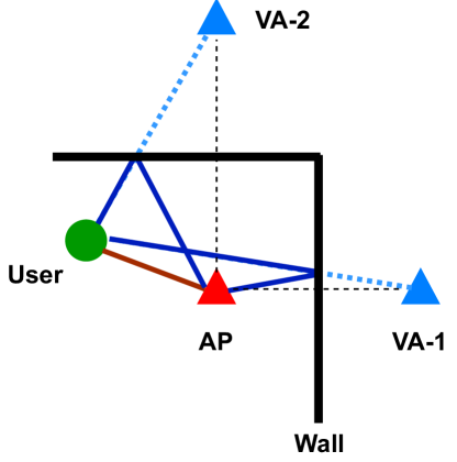
Figure 1: Illustration of the concept of virtual anchor and first-order reflections.

After measuring the angular spectrum from each AP at the client, we elect one reference MPC and compute ADoAs with respect to the AoA of such MPC. If we collect AoA measurements from $N_{a}$ different anchors, we therefore obtain $N_{a}-1$ ADoA values. Using ADoAs values makes the location estimation problem invariant to the client orientation. We employ these ADoAs as the input features of our NN model.

III-C Neural network architecture

Our proposed neural networks consist of three layers: the input layer has $N_{i}=N_{a}-1$ neurons; the first hidden layer contains $N_{h_{1}}$ neurons; the second hidden layer $N_{h_{1}}/2$ neurons; finally, the output layer consists of 2 neurons, one for each of the 2D coordinates of the client. Fig. 2 shows the general structure of the neural network, whereas Table I summarizes the structure of the number of neurons in each layer. Here, $\lceil{\cdot}\rceil$ denotes the ceiling function.

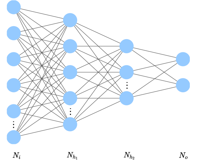
Figure 2: Structure of our proposed NN model.

TABLE I: Summary of the number of neurons in each layer

Layer	Number of neurons
Input layer ($N_{i}$)	$N_{a}-1$
Hidden layer 1 ($N_{h_{1}}$)	$\lceil{N_{i}\cdot k\rceil}$
Hidden layer 2 ($N_{h_{2}}$)	$\lceil N_{h_{1}}/2\rceil$
Output layer ($N_{o}$)	$2$

We train our model to learn the non-linear function that maps the input ADoA data to the output client coordinates. Call ${\bf x}$ the location of the client, and denote the input ADoA vector at location ${\bf x}$ as $\mathbf{a}_{\bf x}$, and the weight matrix of layer $i$, ${\bf W}_{i}$, as

$${\bf W}_{i}=[{\bf w}_{1}\cdots{\bf w}_{n_{i}}]\;,$$ (1)

where $n_{i}$ is the number of neurons in layer $i$, and ${\bf w}_{j}$ is the $n_{i-1}\times 1$ column vector containing the weights of each link that connects the $n_{i-1}$ neurons in the previous layer to the $j$th neuron in the current layer. Moreover, let ${\bf b}_{i}=[b_{1}\cdots b_{n_{i}}]^{T}$ be the vector of bias values for each of the neurons in layer $i$, and call the neuron activation function $A(\cdot)$. Therefore, the output values of layer $i$ are

$$\mathbf{y}_{i}=A({\bf W}_{i}^{T}{\bf y}_{i-1}+\mathbf{b}_{i})\;,$$ (2)

where with a small abuse of notation, applying $A(\cdot)$ to a vector denotes applying $A(\cdot)$ to each entry of the vector. Note that ${\bf y}_{0}={\bf a}_{\bf x}$. Because our NNs have $n=3$ layers, the estimated location of the client is

$$\hat{\bf x}=[\hat{x}_{1},\hat{x}_{2}]^{T}=\mathbf{y}_{3}=\mathcal{F}({\bf a}_{\bf x})\;,$$ (3)

where

$$\mathcal{F}({\bf a}_{\bf x})=A\Big{(}{\bf W}_{3}^{T}A\big{(}{\bf W}_{2}^{T}A({\bf W}_{1}^{T}{\bf a}_{\bf x}+{\bf b}_{1})+{\bf b}_{2}\big{)}+{\bf b}_{3}\Big{)}$$ (4)

is the non-linear regression function applied by the NN. Given the very small number of neurons in our NNs, computing ${\cal F}(\cdot)$ only requires a few simple matrix multiplications and vector summations, making the operation affordable even for computationally-constrained devices. In this work, we choose the rectified linear activation function (ReLU) for $A(\cdot)$, and train the network via the Adam optimizer. As we cast the regression problem as a mean-square error (MSE) minimization problem, we employ the MSE loss function

$$L({\bf x},{\hat{\bf x}})=|x_{1}-\hat{x}_{1}|^{2}+|x_{2}-\hat{x}_{2}|^{2}$$ (5)

where $(x_{1},x_{2})$ are the true location of the user and $(\hat{x}_{1},\hat{x}_{2})$ are the location estimates output by the NN.

We remark that our NN s implement a regression model, i.e., they estimate the coordinates of the client location, rather than identifying which position among multiple possible choices best corresponds to the input data.

III-D Hyperparameter tuning

Through hyperparameter tuning we can optimize the neural network model in order to minimize the loss function. In our model, we tune the following hyperparameters: i) the node factor $k$ which sets the number of neurons in the hidden layers; ii) the dropout rate $p$, which helps avoid overfitting; and iii) the learning rate $r$, which controls the initial speed of convergence. Table II summarizes the hyperparameters used for network model optimization. For the learning rate, we consider a logarithmic progression of values from $10^{-4}$ up to $10^{-2}$, with ten values per decade.

TABLE II: Summary of the hyperparameters chosen to tune our model

Hyperparameter	Range
Node factor ($k$)	$\{0.6,~{}0.7,~{}0.8\}$
Dropout rate ($p$)	$\{0\%,~{}5\%,~{}10\%\}$
Learning rate ($r$)	$[0.0001,0.01]$

IV Simulation results

IV-A Simulation environment and setup

We test our scheme in two indoor environments. The first is a 15$\times$10 m${}^{\textrm{2}}$ rectangular room as shown in Fig. 3a, where three mmWave access points (red squares) are deployed at the coordinates $(4,3)$, $(7.5,6)$ and $(11,3)$, where all values are in meters. Each AP also maps to 4 VAs (blue circles), each corresponding to a different wall.

The second indoor environment is a reverse L-shaped room, whose bottom-left section has size 6$\times$10 m${}^{\textrm{2}}$, whereas the right tall section has size 8$\times$18 m${}^{\textrm{2}}$. Fig. 3b illustrates such L-shaped room. Three APs, placed at coordinates $(4,7)$, $(10,6)$, and $(13,16)$ cover the entire indoor space. As before we depict most VAs as blue circles.

To produce simulation results that are as close to realistic scenarios as possible, we consider the AoA measurements to be affected by zero-mean Gaussian noise of standard deviation error in the set $\{5^{\circ},7^{\circ},10^{\circ}\}$. These values are realistic in mobile user scenarios, given the imperfect beam training procedures and non-pencil-shaped beam patterns of existing commercial off-the-shelf hardware [17].

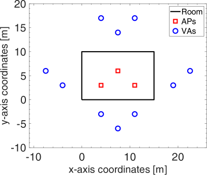
(a) Rectangular room.

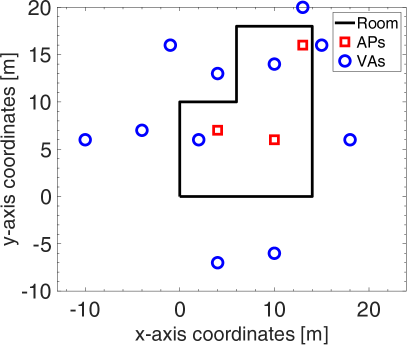
(b) Reverse L-shaped room

Figure 3: Simulation scenarios showing the shape of two rooms, and the location of APs and VAs.

To generate a training set for the NNs, we simulate several mobile client trajectories in each room, and use a ray tracer to collect AoA information at 30 points along each trajectory. Each AoA is affected by a Gaussian-distributed error as explained above. To compare our approach to other algorithms from the literature, we generate a completely different test set of 30 trajectories, for a total of 900 client locations. Note that the train and test dataset are uniformly generated across the entire room.

IV-B Performance evaluation

We start our evaluation by comparing the localization performance of our proposed approach against the JADE [4], Triangulate-Validate (TV), and plain geometric ADoA algorithms [9] from the literature, as they are state-of-the-art approaches relying only on ADoA measurements for location estimation. Fig. 4 shows this comparison for the rectangular room with 3 APs (top panel) as well as with 4 APs, where in the latter case the coordinates of the APs are $(2,1)$, $(4,7)$, $(10,4)$ and $(14,9)$. The figure conveys the statistical dispersion of the location estimation errors for two different values of the standard deviation of AoA errors, $\sigma=5^{\circ}$ and $\sigma=10^{\circ}$. Each box extends from the 1st to the 3rd quartile, the notch denotes the median of the distribution, and the whiskers cover the range from the 10th to the 90th percentiles.

We observe that the dispersion is small both for our NN model and for JADE, whereas TV and ADoA yield larger errors, which increase for higher values of $\sigma$. This is a direct consequence of the geometric operations of the two algorithms, which rely on accurate AoA measurements in order to estimate locations. Instead both JADE and our NN model compensate well for the erroneous angle measurements. However, we remark that the accuracy of JADE comes from having processed a large number of measurements. As this requires to solve minimum mean-square error problems, processing exceedingly many measurements would be very time-consuming. In fact, its complexity increases both with the number of measurements and with the number of APs [4]. Instead, our model learns the mapping between ADoA data and the location of the client, and its complexity remains constant after the training phase (it requires very few multiplications and additions), while achieving equivalent or better accuracy than JADE. With 4 APs (panel b), the general observations remain the same, except that all algorithms yield better estimation errors, with smaller maximum errors, and less statistical dispersion. Because JADE and our NN model outperform TV and ADoA from [9], in the following we will exclude the latter two algorithms from the evaluation.

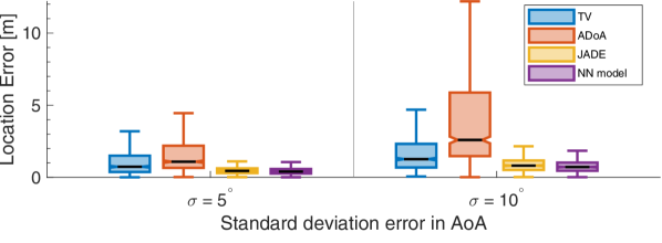
(a) Rectangular room with 3 APs

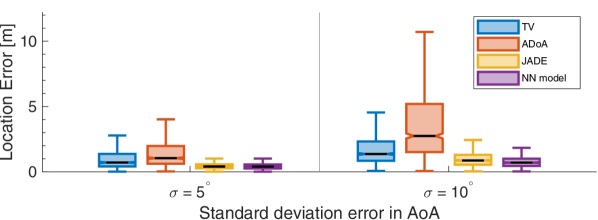
(b) Rectangular room with 4 APs

Figure 4: Statistical dispersion of the localization error for different values of $\sigma$ in the rectangular room with (a) 3 APs and (b) 4 APs.

Fig. 5 shows the reconstruction of a mobile user trajectory using JADE and our NN model, this time in the reverse L-shaped room. The global set of paths considered for our evaluation is shown through grey lines, whereas a thicker blue line conveys the path under consideration. Purple circles convey the estimates of our NN model, whereas green squares represent JADE’s location estimates. For this evaluation, AoAs are affected by errors of standard deviation $\sigma=5^{\circ}$. The resulting NN model has $(18,13,7,2)$ neurons in each layer, and the optimal hyperparameters are $p=0.05$ and $r=0.002$, yielding an MSE of 0.186. We observe that both techniques estimate the locations of the client and reconstruct the corresponding trajectory with good accuracy. The few outliers that remain, both for NN and JADE, are due to erroneous AoA values. Still, our NN model computes estimates closer to the ground-truth trajectory than JADE.

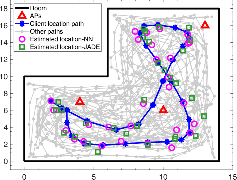
Figure 5: Path reconstruction in the L-shaped room using our neural network model and JADE. $\sigma=5^{\circ}$. Axis tick labels are in meters.

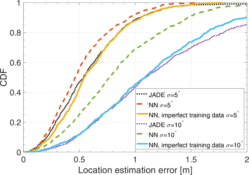
Figure 6: Cumulative distribution function of the location error for our NN approach against JADE in the L-shaped room environment. The NNs are trained both with perfect and with error-prone data.

IV-C Training the NNs with estimated user locations

We now consider the case where we train our NN with imperfect location labels from the JADE algorithm, which is inherently error-prone. The performance of the proposed method is illustrated in Fig. 6 through the cumulative distribution function (CDF) of the location error for different approaches, evaluated in the L-shaped room. The NNs trained with imperfect labels have $(18,13,7,2)$ neurons in each stage. For $\sigma=5^{\circ}$, the optimal hyperparameters are $p=0$ and $r=0.006$, whereas $p=0.05$ and $r=0.0004$ for $\sigma=10^{\circ}$.

We observe that the NNs trained with JADE estimates (solid blue and yellow curves) perform just as good as JADE when $\sigma=5^{\circ}$, and even better if $\sigma=10^{\circ}$. This supports our intuition that collecting error-prone training samples does not significantly deteriorate the location estimates of our NN models. In particular, for $\sigma=5^{\circ}$, training the NNs with imperfect data from JADE yields sub-meter errors in 88% of the cases, and a median error of 0.47 m. This compares very well to the 92% sub-meter errors and the median error of 0.45 m achieved with perfectly labeled training data.

IV-D Impact of number of training samples

We conclude our study by assessing the performance of our model as a function of the training set size. As presented in [4], the complexity of JADE increases as the mmWave client keeps collecting angular spectrum measurements. Thus, we can run JADE up to a point where its complexity does not become excessive. To validate this with our proposed scheme, we consider training datasets including 250, 750, and 1200 samples. We then train our model both with perfect locations labels and with imperfect location estimates from JADE. Fig. 7 compares the corresponding box plots for $\sigma=5^{\circ}$ and $\sigma=7^{\circ}$. The results show that both the median location error and the statistical dispersion of the error decrease by increasing the number of training samples. This is true even when the model is trained with JADE’s estimates, as such estimates become more accurate when computed from a larger set of measurements [4]. This confirms that our NN model can be trained with a significantly small number of training samples compared to DNN models, and that the resulting errors are acceptable even when training samples are error-prone.

We remark that two trends emerge from the figure. On the one hand, with a comparatively small training set (blue and red boxes), the NN may underfit the map between angular spectra and the device location: in this regime, training with imperfect estimates only marginally increases the localization error of the NN. On the other hand, for a large training dataset (green and light-blue boxes), the environment is well sampled, and JADE’s estimates are quite accurate. Therefore, training with error-prone location labels yields almost the same accuracy as training with true locations. Between these two regimes, training with true locations (yellow box) expectedly yields better performance than training with JADE’s location estimates (purple box). The system designer may therefore trade off localization performance with the number of samples retrieved from JADE before switching to the NN model.

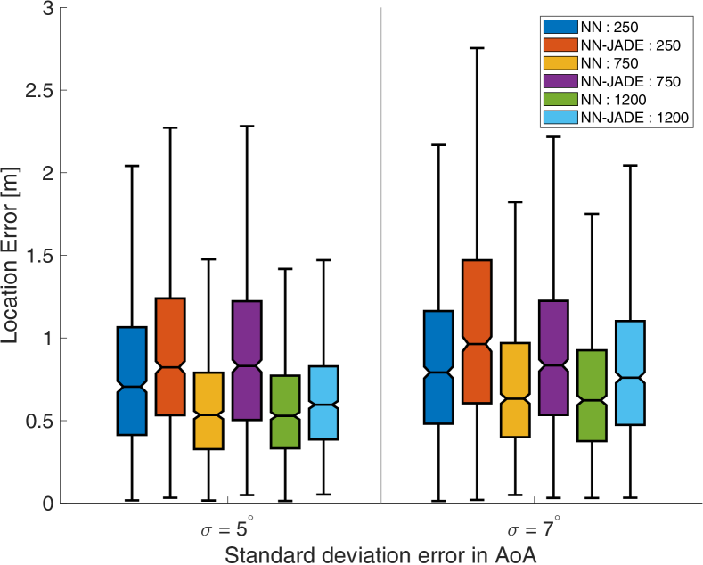
Figure 7: Statistical dispersion of the localization error for different number of training samples and values of $\sigma$, when the NN is trained with true user locations (key: NN) and with estimates from JADE (key: NN-JADE).

V Conclusions and future work

In this paper, we proposed a shallow neural network model that localizes a client in an indoor environment. The model uses ADoA values as input and can be trained through error-prone client location estimates from a mmWave localization algorithm, in order to relieve the training dataset collection effort. Our performance evaluation suggests that the NN model achieves a high degree of accuracy when trained with perfect data, in spite of its shallowness, even in the presence of significant AoA estimation errors. Such accuracy does not significantly degrade when trained with imperfect location labels. Results show sub-meter localization accuracy in $\approx 90\%$ of the scenarios with large AoA errors. Future work includes the experimental validation of the proposed method using mmWave COTS devices.

References

- [1] S. Rangan, T. S. Rappaport, and E. Erkip, “Millimeter-wave cellular wireless networks: Potentials and challenges,” Proceedings of the IEEE, vol. 102, no. 3, pp. 366–385, 2014.
- [2] K. Sakaguchi et al., “Where, When, and How mmWave is Used in 5G and Beyond,” IEICE Transactions on Electronics, vol. E100.C, 04 2017.
- [3] T. S. Rappaport et al., “Millimeter wave mobile communications for 5G cellular: It will work!” IEEE Access, vol. 1, pp. 335–349, 2013.
- [4] J. Palacios, P. Casari, and J. Widmer, “JADE: Zero-knowledge device localization and environment mapping for millimeter wave systems,” in Proc. IEEE INFOCOM, 2017, pp. 1–9.
- [5] J. Palacios et al., “Communication-driven localization and mapping for millimeter wave networks,” in Proc. IEEE INFOCOM, Apr. 2018.
- [6] T. Koike-Akino et al., “Fingerprinting-based indoor localization with commercial mmWave WiFi: A deep learning approach,” IEEE Access, vol. 8, pp. 84 879–84 892, 2020.
- [7] P. Wang, T. Koike-Akino, and P. V. Orlik, “Fingerprinting-based indoor localization with commercial mWave WiFi: NLOS propagation,” in Proc. IEEE GLOBECOM, 2020, pp. 1–6.
- [8] A. Olivier et al., “Lightweight indoor localization for 60-GHz millimeter wave systems,” in Proc. IEEE SECON, 2016, pp. 1–9.
- [9] J. Palacios et al., “Single-and multiple-access point indoor localization for millimeter-wave networks,” IEEE Trans. Wireless Commun., vol. 18, no. 3, pp. 1927–1942, 2019.
- [10] I. Pefkianakis and K.-H. Kim, “Accurate 3D localization for 60 GHz networks,” in Proc. ACM SenSys, 2018, pp. 120–131.
- [11] J. Palacios et al., “LEAP: Location estimation and predictive handover with consumer-grade mmwave devices,” in Proc. IEEE INFOCOM, 2019, pp. 2377–2385.
- [12] O. Kanhere et al., “Map-assisted millimeter wave localization for accurate position location,” in Proc. IEEE GLOBECOM, 2019, pp. 1–6.
- [13] A. Vashist et al., “Indoor wireless localization using consumer-grade 60 GHz equipment with machine learning for intelligent material handling,” in Proc. IEEE ICCE, 2020, pp. 1–6.
- [14] M. Pajovic et al., “Fingerprinting-based indoor localization with commercial mmWave WiFi - part I: RSS and beam indices,” in Proc. IEEE GLOBECOM, 2019, pp. 1–6.
- [15] P. Wang et al., “Fingerprinting-based indoor localization with commercial mmwave WiFi - part II: Spatial beam SNRs,” in Proc. IEEE GLOBECOM, 2019, pp. 1–6.
- [16] K. He et al., “Deep residual learning for image recognition,” 2015, arXiv preprint 1512.03385.
- [17] D. Steinmetzer et al., “Compressive millimeter-wave sector selection in off-the-shelf IEEE 802.11ad devices,” in Proc. ACM CoNEXT, 2017.