PARL: Enhancing Diversity of Ensemble Networks to Resist Adversarial Attacks via Pairwise Adversarially Robust Loss Function

Abstract

The security of Deep Learning classifiers is a critical field of study because of the existence of adversarial attacks. Such attacks usually rely on the principle of transferability, where an adversarial example crafted on a surrogate classifier tends to mislead the target classifier trained on the same dataset even if both classifiers have quite different architecture. Ensemble methods against adversarial attacks demonstrate that an adversarial example is less likely to mislead multiple classifiers in an ensemble having diverse decision boundaries. However, recent ensemble methods have either been shown to be vulnerable to stronger adversaries or shown to lack an end-to-end evaluation. This paper attempts to develop a new ensemble methodology that constructs multiple diverse classifiers using a Pairwise Adversarially Robust Loss (PARL) function during the training procedure. PARL utilizes gradients of each layer with respect to input in every classifier within the ensemble simultaneously. The proposed training procedure enables PARL to achieve higher robustness against black-box transfer attacks compared to previous ensemble methods without adversely affecting the accuracy of clean examples. We also evaluate the robustness in the presence of white-box attacks, where adversarial examples are crafted using parameters of the target classifier. We present extensive experiments using standard image classification datasets like CIFAR-10 and CIFAR-100 trained using standard ResNet20 classifier against state-of-the-art adversarial attacks to demonstrate the robustness of the proposed ensemble methodology.

1 Introduction

Deep learning (DL) algorithms have seen rapid growth in recent years because of their unprecedented successes with near-human accuracies in a wide variety of challenging tasks starting from image classification [38], speech recognition [2], natural language processing [40] to self-driving cars [6]. While DL algorithms are extremely efficient in solving complicated decision-making tasks, they are vulnerable to well-crafted adversarial examples (slightly perturbed valid input with visually imperceptible noise) [37]. The widely-studied phenomenon of adversarial examples among the research community has produced numerous attack methodologies with varied complexity and effective deceiving strategy [12, 24, 27, 29, 32]. An extensive range of defenses against such attacks has been proposed in the literature, which generally falls into two categories. The first category enhances the training strategy of deep learning models to make them less vulnerable to adversarial examples by training the models with different degrees of adversarially perturbed training data [4, 18, 19, 42] or changing the training procedure like gradient masking, defensive distillation, etc. [15, 31, 34, 35]. However, developing such defenses has been shown to be extremely challenging. Carlini and Wagner [8] demonstrated that these defenses are not generalized for all varieties of adversarial attacks but are constrained to specific categories. The process of training with adversarially perturbed data is hard, often requires models with large capacity, and suffers from significant loss on clean example accuracy. Moreover, Athalye et al. [3] demonstrated that the changes in training procedures provide a false sense of security. The second category intends to detect adversarial examples by simply flagging them [5, 10, 11, 14, 28, 17, 25]. However, even detection of adversarial examples can be quite a complicated task. Carlini and Wagner [7] illustrated with several experimentations that these detection techniques could be efficiently bypassed by a strong adversary having partial or complete knowledge of the internal working procedure.

While all the approaches mentioned above deal with standalone classifiers, in this paper, we utilize the advantage of an ensemble of classifiers instead of a single standalone classifier to resist adversarial attacks. The notion of using diverse ensembles to increase the robustness of a classifier against adversarial examples has recently been explored in the research community. The primary motivation of using an ensemble-based defense is that if multiple classifiers with similar decision boundaries perform the same task, the transferability property of DL classifiers makes it easier for an adversary to mislead all the classifiers simultaneously using adversarial examples crafted on any of the classifiers. However, it will be difficult for an adversary to mislead multiple classifiers simultaneously if they have diverse decision boundaries. Strauss et al. [36] used various ad-hoc techniques such as different random initializations, different neural network structures, bagging the input data, adding Gaussian noise while training for creating multiple diverse classifiers to form an ensemble. The resulting ensemble increases the robustness of the classification task even in the presence of adversarial examples. Tramèr et al. [39] proposed Ensemble Adversarial Training that incorporates perturbed inputs transferred from other pre-trained models during adversarial training to decouple adversarial example generation from the parameters of the primary model. Grefenstette et al. [13] demonstrated that ensembling two models and then adversarially training them incorporates more robustness in the classification task than single-model adversarial training and ensemble of two separately adversarially trained models. Kariyappa and Qureshi [20] proposed Diversity Training of an ensemble of models with uncorrelated loss functions using Gradient Alignment Loss metric to reduce the dimension of adversarial sub-space shared between different models and increase the robustness of the classification task. Pang et al. [30] proposed Adaptive Diversity Promoting regularizer to train an ensemble of classifiers that encourages the non-maximal predictions in each member in the ensemble to be mutually orthogonal, which degenerates the transferability that aids in resisting adversarial examples. Yang et al. [41] proposed a methodology that isolates the adversarial vulnerability in each sub-model of an ensemble by distilling non-robust features. While all these works attempt to enhance the robustness of a classification task even in the presence of adversarial examples, Adam et al. [1] proposed a stochastic method to add Variational Autoencoders between layers as a noise removal operator for creating combinatorial ensembles to limit the transferability and detect adversarial examples.

In order to enhance the robustness of a classification task and/or to detect adversarial examples, the ensemble-based approaches mentioned above employ different strategies while training the models. These ensembles either lack end-to-end evaluations for complicated datasets or lack evaluation against more aggressive attack scenarios like the methods discussed by Dong et al. [9] and Liu et al. [26], which demonstrate that adversarial examples misleading multiple models in an ensemble tend to be more transferable. In this work, our primary objective is to propose a systematic approach to enhance the classification robustness of an ensemble of classifiers against adversarial examples by developing diversity in the decision boundaries among all the classifiers within that ensemble. The diversity is obtained by simultaneously considering the mutual dissimilarity in gradients of each layer with respect to input in every classifier while training them. The diversity among the classifiers trained in such a way helps to degenerate the transferability of adversarial examples within the ensemble.

Motivation behind the Proposed Approach and Contribution: The intuition behind developing the proposed ensemble methodology is discussed in Figure 1, which shows a case study using classifiers trained on CIFAR-10 dataset without loss of generality. Figure 1a shows an input image of a ‘frog’. Figure 1b shows the gradient of loss with respect to input in a classifier $\mathcal{M}_{prim}$, and denoted as $\nabla_{prim}$. Figure 1c shows the gradient for another classifier $\mathcal{M}_{sim}$ with a similar decision boundary as $\mathcal{M}_{prim}$, and denoted as $\nabla_{sim}$. The classifier $\mathcal{M}_{sim}$ is trained using the same parameter settings as $\mathcal{M}_{prim}$ but with different random initialization. Figure 1d shows the gradients for a classifier $\mathcal{M}_{div}$ with a not so similar decision boundary compared to $\mathcal{M}_{prim}$, and denoted as $\nabla_{div}$. The classifiers $\mathcal{M}_{prim}$, $\mathcal{M}_{sim}$, and $\mathcal{M}_{div}$ have similar classification accuracies. The method for obtaining such classifiers is discussed later in this paper. Figure 1e shows relative symbolic directions among all the aforementioned gradients in higher dimension. The directions between a pair of gradients are computed using cosine similarity. We can observe that $\nabla_{prim}$ and $\nabla_{sim}$ lead to almost in the same directions, aiding adversarial examples crafted on $\mathcal{M}_{prim}$ to transfer into $\mathcal{M}_{sim}$. However, adversarial examples crafted in $\mathcal{M}_{prim}$ will be difficult to transfer into $\mathcal{M}_{div}$ as the directions of $\nabla_{prim}$ and $\nabla_{div}$ are significantly different.

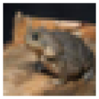
(a)

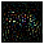
(b)

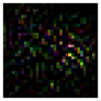
(c)

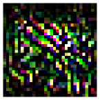
(d)

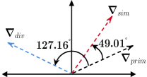
(e)

Figure 1: (a) Input image; (b) $\nabla_{prim}$: Gradient of loss in the primary classifier; (c) $\nabla_{sim}$: Gradient of loss in another classifier with similar decision boundaries; (d) $\nabla_{div}$: Gradient of loss in a classifier with not so similar decision boundaries but comparable accuracy; (e) Symbolic directions of all the gradients in higher dimensions. The gradients are computed with respect to the image shown in (a).

The principal motivation behind the proposed methodology is to introduce a constraint for reducing the cosine similarity of gradients among each classifier in an ensemble while training them simultaneously. Such a learning strategy with mutual cooperation intends to ensure that gradients between each pair of classifiers in the ensemble are as dissimilar as possible. We make the following contributions using the proposed ensemble training method:

• We propose a methodology to increase diversity in the decision boundaries among all the classifiers within an ensemble to degrade the transferability of adversarial examples.

• We propose a Pairwise Adversarially Robust Loss (PARL) function by utilizing the gradients of each layer with respect to input of every classifier within the ensemble simultaneously for training them to produce such varying decision boundaries.

• The proposed method can significantly improve the overall robustness of the ensemble against black-box transfer attacks without substantially impacting the clean example accuracy.

• We evaluated the robustness of PARL with extensive experiments using two standard image classification benchmark datasets on ResNet20 architecture against state-of-the-art adversarial attacks.

2 Threat Model

We consider the following two threat models in this paper while generating adversarial examples.

• Zero Knowledge Adversary $(\mathcal{A}_{\mathcal{Z}})$: The adversary $\mathcal{A}_{\mathcal{Z}}$ does not have access to the target ensemble $\mathcal{M}_{\mathcal{T}}$ but has access to a surrogate ensemble $\mathcal{M}_{\mathcal{S}}$ trained with the same dataset. We term $\mathcal{A}_{\mathcal{Z}}$ as a black-box adversary. The adversary $\mathcal{A}_{\mathcal{Z}}$ crafts adversarial examples on $\mathcal{M}_{\mathcal{S}}$ and transfers to $\mathcal{M}_{\mathcal{T}}$.

• Perfect Knowledge Adversary $(\mathcal{A}_{\mathcal{P}})$: The adversary $\mathcal{A}_{\mathcal{P}}$ is a stronger than $\mathcal{A}_{\mathcal{Z}}$ who has access to the target ensemble $\mathcal{M}_{\mathcal{T}}$. We term $\mathcal{A}_{\mathcal{P}}$ as a white-box adversary. The adversary $\mathcal{A}_{\mathcal{P}}$ can generate adversarial examples on $\mathcal{M}_{\mathcal{T}}$ knowing the parameters used by all the networks within $\mathcal{M}_{\mathcal{T}}$ .

3 Overview of the Proposed Methodology

In this section, we provide a brief description of the proposed methodology used in this paper to enhance classification robustness against adversarial examples using an ensemble of classifiers $\mathcal{M}_{\mathcal{T}}$. The ensemble consists of $\mathcal{N}$ neural network classifiers and denoted as $\mathcal{M}_{\mathcal{T}}=\bigcup_{i=1}^{\mathcal{N}}\mathcal{M}_{i}$. All the $\mathcal{M}_{i}$’s are trained simultaneously using the Pairwise Adversarially Robust Loss (PARL) function, which we discuss in detail in Section 4. The final decision for an input image on $\mathcal{M}_{\mathcal{T}}$ is decided based on the majority voting among all the classifiers. Formally, let us assume a test set of $t$ inputs $\{x_{1},x_{2},\dots,x_{t}\}$ with respective ground truth labels as $\{y_{1},y_{2},\dots,y_{t}\}$. The final decision of the ensemble $\mathcal{M}_{\mathcal{T}}$ for an input $x_{j}$ is defined as

$$\mathcal{C}(\mathcal{M}_{\mathcal{T}},x_{j})=majority\{\mathcal{M}_{1}(x_{j}),\mathcal{M}_{2}(x_{j}),\cdots,\mathcal{M}_{\mathcal{N}}(x_{j})\}$$

$\mathcal{C}(\mathcal{M}_{\mathcal{T}},x_{j})=y_{j}$ for most $x_{j}$’s in an appropriately trained $\mathcal{M}_{\mathcal{T}}$. The primary argument behind the proposed ensemble method is that all $\mathcal{M}_{i}$’s have dissimilar decision boundaries but not significantly different accuracies. Hence, a clean example classified as class $\mathcal{C}_{x}$ in $\mathcal{M}_{i}$ will also be classified as $\mathcal{C}_{x}$ in most other $\mathcal{M}_{j}$’s (where $j=1\dots\mathcal{N}$, $j\neq i$) within the ensemble with a high probability. Consequently, because of the diversity in decision boundaries between $\mathcal{M}_{i}$ and $\mathcal{M}_{j}$ (for $i=1\dots\mathcal{N}$, $j=1\dots\mathcal{N}$, and $i\neq j$), the adversarial examples generated by a zero knowledge adversary $(\mathcal{A}_{\mathcal{Z}})$ for a surrogate ensemble $\mathcal{M}_{\mathcal{S}}$ will have a different impact on each classifiers within the ensemble $\mathcal{M}_{\mathcal{T}}$, i.e., the transferability of adversarial examples will be challenging within the ensemble. A perfect knowledge adversary $(\mathcal{A}_{\mathcal{P}})$ can generate adversarial examples for the ensemble $\mathcal{M}_{\mathcal{T}}$. However, in this scenario, the input image perturbation will be in different directions because of the diversity in decision boundaries among all $\mathcal{M}_{i}$’s within the ensemble. The collective disparity in perturbation directions makes it challenging to craft adversarial examples for the ensemble. We evaluated our proposed methodology considering both the adversaries and presented the results in Section 5.

4 Building The Ensemble Networks using PARL

In this section, we provide a detailed discussion on training an ensemble of neural networks using the proposed Pairwise Adversarially Robust Loss (PARL) function for increasing diversity among the networks. First, we define the basic terminologies used in the construction, followed by a detailed methodology of the training procedure.

4.1 Basic Terminologies used in the Construction

Let us consider an ensemble $\mathcal{M}_{\mathcal{T}}=\bigcup_{i=1}^{\mathcal{N}}\mathcal{M}_{i}$, where $\mathcal{M}_{i}$ is the $i^{th}$ network in the ensemble. We assume that each of these networks has the same architecture with $\mathcal{L}_{\mathcal{H}}$ number of hidden layers. Let $\mathcal{J}_{\mathcal{M}_{i}}(\mathbf{x},\mathbf{y})$ be the loss functions evaluating the amount of loss incurred by the network $\mathcal{M}_{i}$ for a data point $\mathbf{x}$, where $\mathbf{y}$ is the ground-truth label for $\mathbf{x}$. Let $\mathcal{F}^{\mathcal{L}_{k}}_{\mathcal{M}_{i}}(\mathbf{x})$ be the output of $k^{th}$ hidden layer on the network $\mathcal{M}_{i}$ for the data point $\mathbf{x}$. Let us assume $\mathcal{F}^{\mathcal{L}_{k}}_{\mathcal{M}_{i}}(\mathbf{x})$ has $\mathcal{D}(\mathcal{L}_{k})$ number of output features. Let us consider $\nabla_{x}\mathcal{F}^{\mathcal{L}_{k}}_{\mathcal{M}_{i}}(\mathbf{x})$ denote the sum of gradients over each output feature of $k^{th}$ hidden layer with respect to input on the network $\mathcal{M}_{i}$ for the data point $\mathbf{x}$. Hence,

$$\nabla_{x}\mathcal{F}^{\mathcal{L}_{k}}_{\mathcal{M}_{i}}(\mathbf{x})=\sum_{f=1}^{\mathcal{D}(\mathcal{L}_{k})}\nabla_{x}[\mathcal{F}^{\mathcal{L}_{k}}_{\mathcal{M}_{i}}(\mathbf{x})]_{f}$$

where $\nabla_{x}[\mathcal{F}^{\mathcal{L}_{k}}_{\mathcal{M}_{i}}(\cdot)]_{f}$ is the gradient of the $f^{th}$ output feature of $k^{th}$ hidden layer on network $\mathcal{M}_{i}$ with respect to input for the data point $\mathbf{x}$. Let $\mathcal{X}$ be the training dataset containing $|\mathcal{X}|$ examples.

4.2 Pairwise Adversarially Robust Loss Function

The principal idea behind the proposed approach is to train an ensemble of neural networks such that the gradients of loss with respect to input in all the networks will be in different directions. The gradients represent the directions in which the input needs to be perturbed such that the loss of the network increases, helping to transfer adversarial examples. In this paper, we introduce the Pairwise Adversarially Robust Loss (PARL) function, which we will use to train the ensemble. The objective of PARL is to train the ensemble so that the gradients of loss lead to different directions in different networks for the same input example. Hence, the fundamental strategy is to make the gradients as dissimilar as possible while training all the networks. Since the gradient computation depends on all intermediate parameters of a network, we force the intermediate layers of all the networks within the ensemble to be dissimilar for producing enhanced diversity at each layer.

The pairwise similarity of gradients of the output of $k^{th}$ hidden layer with respect to input between the classifiers $\mathcal{M}_{i}$ and $\mathcal{M}_{j}$ for a particular data point $\mathbf{x}$ can be represented as

$$\mathcal{G}_{\mathcal{L}_{k}}^{(i,j)}(\mathbf{x})=\frac{<\nabla_{x}\mathcal{F}^{\mathcal{L}_{k}}_{\mathcal{M}_{i}}(\mathbf{x}),\nabla_{x}\mathcal{F}^{\mathcal{L}_{k}}_{\mathcal{M}_{j}}(\mathbf{x})>}{\|\nabla_{x}\mathcal{F}^{\mathcal{L}_{k}}_{\mathcal{M}_{i}}(\mathbf{x})\|\cdot\|\nabla_{x}\mathcal{F}^{\mathcal{L}_{k}}_{\mathcal{M}_{j}}(\mathbf{x})\|}$$

where $<a,b>$ represents the dot product between two vectors $a$ and $b$. The overall pairwise similarity between the classifiers $\mathcal{M}_{i}$ and $\mathcal{M}_{j}$ for a particular data point $\mathbf{x}$ considering $\mathcal{L}_{\mathcal{H}}$ hidden layers can be written as

$$\mathcal{G}^{(i,j)}(\mathbf{x})=\sum_{k=1}^{\mathcal{H}}\mathcal{G}_{\mathcal{L}_{k}}^{(i,j)}(\mathbf{x})$$

Next, we define a penalty term $\mathcal{R}(\mathcal{M}_{i},\mathcal{M}_{j})$ for all the training examples in $\mathcal{X}$ to pairwise train the models $\mathcal{M}_{i}$ and $\mathcal{M}_{j}$ as

$$\mathcal{R}(\mathcal{M}_{i},\mathcal{M}_{j})=\frac{1}{|\mathcal{X}|}\sum_{\mathbf{x}\in\mathcal{X}}\mathcal{G}^{(i,j)}(\mathbf{x})$$

We can observe that $\mathcal{R}$ computes average pairwise similarity for all the training examples. Now, for network $\mathcal{M}_{i}$ and $\mathcal{M}_{j}$, if all the gradients with respect to input for each training example are in the same direction, value of $\mathcal{R}$ will be close to $1$, indicating similarity in decision boundaries. The value of $\mathcal{R}$ will gradually decrease as the relative angle between the pair of gradients increases in higher dimension. Hence, the objective of diversity training using PARL is to reduce the value of $\mathcal{R}$. Thus, we add $\mathcal{R}$ to the loss function as a penalty parameter to penalize the training for a large $\mathcal{R}$ value.

In the ensemble $\mathcal{M}_{\mathcal{T}}$, we compute the $\mathcal{R}$ values for each distinct pair of $\mathcal{M}_{i}$ and $\mathcal{M}_{j}$ in order to enforce diversity between each pair of classifiers. We define PARL to train the ensemble $\mathcal{M}_{\mathcal{T}}$ as

$$PARL(\mathcal{M}_{\mathcal{T}})=\gamma_{1}\cdot\frac{1}{|\mathcal{X}|}\sum_{\mathbf{x}\in\mathcal{X}}\sum_{i=1}^{\mathcal{N}}J_{\mathcal{M}_{i}}(\mathbf{x},\mathbf{y})+\gamma_{2}\cdot\sum_{1\leq i<j\leq\mathcal{N}}\mathcal{R}(\mathcal{M}_{i},\mathcal{M}_{j})$$ (1)

where $\gamma_{1}$ and $\gamma_{2}$ are hyperparameters controlling the accuracy-robustness trade-off. A higher value of $\gamma_{1}$ and a lower value of $\gamma_{2}$ helps to learn the models with good accuracy but is less robust against adversarial attacks. However, a lower value of $\gamma_{1}$ and a higher value of $\gamma_{2}$ makes the models more robust against adversarial attacks but with a compromise in overall accuracy.

One may note that the inclusion of the penalty values for each distinct pair of classifiers within the ensemble to compute PARL has one fundamental advantage. If we do not include the pair $(\mathcal{M}_{a},\mathcal{M}_{b})$ in the PARL computation, the training will continue without any diversity restrictions between $\mathcal{M}_{a}$ and $\mathcal{M}_{b}$. Consequently, $\mathcal{M}_{a}$ and $\mathcal{M}_{b}$ will produce similar decision boundaries, thereby increasing the likelihood of adversarial transferability between $\mathcal{M}_{a}$ and $\mathcal{M}_{b}$, affecting the robustness of the ensemble $\mathcal{M}_{\mathcal{T}}$. One may also note that the number of gradient computations in an efficient implementation of PARL is linearly proportional to the number of classifiers in the ensemble. The gradients for each classifier are computed once and are reused to compute $\mathcal{R}$ values for each pair of classifiers. The reuse of gradients protects the implementation from the exponential computational overhead due to pairwise similarity computation.

5 Experimental Evaluation

5.1 Evaluation Configurations

We consider an ensemble of three standard ResNet20 [16] architecture for all the ensembles used in this paper. We consider two standard image classification datasets for our evaluation, namely CIFAR-10 [23] and CIFAR-100 [23]. We consider two scenarios for the evaluation:

• Unprotected Ensemble: A baseline ensemble $(ENS_{\mathcal{U}})$ of ResNet20 architectures without any countermeasure against adversarial attacks.

• Protected Ensemble: An ensemble $(ENS_{\mathcal{Z}})$ of ResNet20 architectures, where $\mathcal{Z}$ is the countermeasure used to design the ensemble. In our evaluation we have considered three previously proposed countermeasures to compare the performance of PARL. We denote the ensembles $ENS_{ADP}$, $ENS_{GAL}$, and $ENS_{DVERGE}$ to be the ensembles trained with the methods proposed by Pang et al. [30], Kariyappa and Qureshi [20], and Yang et al. [41], respectively. The ensemble trained with our proposed method is denoted as $ENS_{PARL}$.

We use the adam optimization [21] to train all the ensembles with adaptive learning rate starting from $0.001$. We dynamically generate a augmented dataset using random shifts, flips and crops to train both CIFAR-10 and CIFAR-100. We use the default hyperparameter settings mentioned in the respective papers for $ENS_{ADP}$, $ENS_{GAL}$, and $ENS_{DVERGE}$. We use $\gamma_{1}=1.0$, $\gamma_{2}=0.5$, and categorical crossentropy loss for $\mathcal{J}_{\mathcal{M}_{i}}(\cdot)$ (ref. Equation (1)) for $ENS_{PARL}$. We enforce diversity among all the classifiers in $ENS_{PARL}$ for the first seven convolution layers.

We consider four state-of-the-art untargeted adversarial attacks Fast Gradient Sign Method (FGSM) [12], Basic Iterative Method (BIM) [24], Momentum Iterative Method (MIM) [9], and Projected Gradient Descent (PGD) [27] for crafting adversarial examples. A brief overview on crafting adversarial examples using these attack methodologies are discussed in Appendix A. We consider 50 steps for generating adversarial examples using the iterative methods BIM, MIM, and PGD with the step size of $\epsilon/5$, where $\epsilon$ is the attack strength. We consider the moment decay factor as $0.01$ for MIM. We use $10$ different random restarts for PGD to generate multiple instances of adversarial examples for an impartial evaluation. We use $\epsilon=0.01,0.02,0.03,0.04,0.05,0.06$, and $0.07$ for generating adversarial examples of different strengths. We use CleverHans v2.1.0 library [33] to generate all the adversarial examples.

In order to evaluate against a stronger adversarial setting for $\mathcal{A}_{\mathcal{Z}}$, we train a black-box surrogate ensemble and generate adversarial examples from the surrogate ensemble instead of a standalone classifier. As also mentioned previously, adversarial examples that mislead multiple models in an ensemble tend to be more transferable [9, 26]. All the results in the subsequent discussions are reported by taking average value over three independent runs.

5.2 Analysing the Diversity

The primary objective of PARL is to increase the diversity among all the classifiers within an ensemble. In order to analyze the diversity of different classifiers trained using PARL, we use Linear Central Kernel Alignment (CKA) analysis proposed by Kornblith et al. [22]. The CKA metric, which lies between $[0,1]$, measures the similarity between decision boundaries represented by a pair of neural networks. A higher CKA value between two neural networks indicates a significant similarity in decision boundary representations, which implies good transferability of adversarial examples. We present an analysis on layer-wise CKA values for each pair of classifiers within the ensemble $ENS_{\mathcal{U}}$ and $ENS_{PARL}$ trained with CIFAR-10 and CIFAR-100 in Figure 2 to show the effect of PARL on diversity.

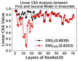
(a)

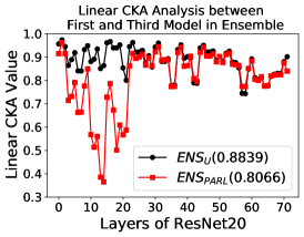
(b)

(c)

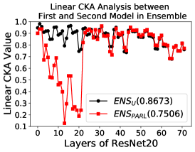
(d)

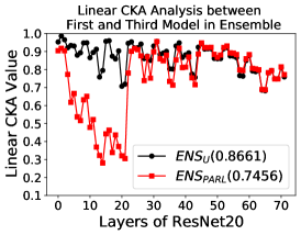
(e)

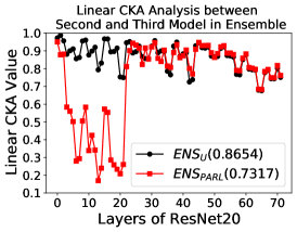
(f)

Figure 2: Layer-wise linear CKA values between each pair of classifiers in $ENS_{\mathcal{U}}$ and $ENS_{PARL}$ trained with CIFAR-10 [(a), (b), (c)] and CIFAR-100 [(d), (e), (f)] datasets showing the similarities at each layer. The value inside the braces within the corresponding figure legends represent the overall average Linear CKA values between each pair of classifiers.

We can observe that each pair of models in $ENS_{\mathcal{U}}$ show a significant similarity at every layer. However, since $ENS_{PARL}$ is trained by restricting the first seven convolution layers, we can observe a considerable decline in the CKA values at the initial layers. The observation is expected as $PARL$ imposes layer-wise diversity in its formulation, as discussed previously in Section 4. The overall average Linear CKA values between each pair of models in Figure 2 are mentioned inside braces within the corresponding figure legends, which signifies that the classifiers within an ensemble trained using PARL shows a higher overall dissimilarity than the unprotected baseline ensemble. In the subsequent discussions, we analyze the effect of the observed diversity on the performance of $ENS_{PARL}$ against adversarial examples.

5.3 Robustness Evaluation of PARL

Performance in the presence of $\mathcal{A}_{\mathcal{Z}}$: We evaluate the robustness of all the ensembles discussed in Section 5.1 considering both CIFAR-10 and CIFAR-100 where the attackers cannot access the model parameters and rely on surrogate models to generate transferable adversarial examples. Under such a black-box scenario, we use one hold-out ensemble with three ResNet20 models as the surrogate model. We randomly select 1000 test samples and evaluate the performance of black-box transfer attacks for all the ensembles across a wide range of attack strength $\epsilon$. We present the result for the attack strength ($\epsilon=0.07$) in Table 1 along with clean example accuracies. The methods presented by Kariyappa and Qureshi [20] and [41] neither evaluated their approach on a more complicated CIFAR-100 dataset nor discussed any optimal hyperparameter settings regarding their proposed algorithms for potential evaluation. In our robustness evaluations, we consider all the ensembles discussed in Section 5.1 for CIFAR-10. In contrast, we only consider $ENS_{\mathcal{U}}$ and $ENS_{ADP}$ to compare the performance of $ENS_{PARL}$ for CIFAR-100. We can observe from Table 1 that the training using PARL does not adversely affect the ensemble accuracy on clean examples compared to other previously proposed methodologies. However, it provides better robustness against black-box transfer attacks for almost every scenario.

Table 1: Ensemble classification accuracy (%) for CIFAR-10 and CIFAR-100 on clean examples as well as adversarially perturbed images with attack strength $\epsilon=0.07$ for different adversarial attacks.

		Clean Example	FGSM	BIM	MIM	PGD
$ENS_{\mathcal{U}}$	CIFAR-10	93.11	21.87	7.47	7.27	1.57
	CIFAR-100	70.88	7.13	7.17	3.93	5.39
$ENS_{ADP}$	CIFAR-10	92.99	23.53	8.13	7.53	3.08
	CIFAR-100	70.01	8.23	10.07	5.83	8.72
$ENS_{GAL}$	CIFAR-10	91.22	22.8	9.3	8.33	7.64
	CIFAR-100	*	*	*	*	*
$ENS_{DVERGE}$	CIFAR-10	91.73	28.88	11.78	10.55	9.68
	CIFAR-100	*	*	*	*	*
$ENS_{PARL}$	CIFAR-10	91.09	28.37	20.8	16.17	15.65
	CIFAR-100	67.52	12.73	18.97	10.01	21.49

• * Did not consider CIFAR-100 dataset for evaluation

A more detailed performance evaluation considering all the attack strengths are presented in Figure 3. For CIFAR-10 evaluation (ref. Figure 3a - Figure 3d), we can observe that $ENS_{PARL}$ performs at par with $ENS_{DVERGE}$ considering FGSM. However, for stronger iterative attacks like BIM, MIM, and PGD, $ENS_{PARL}$ outperforms other methodologies with higher accuracy for large attack strengths. For CIFAR-100 evaluation (ref. Figure 3e - Figure 3h), we can observe that $ENS_{PARL}$ performs better than both $ENS_{\mathcal{U}}$ and $ENS_{ADP}$ for all scenarios.

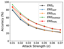
(a) FGSM

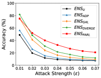
(b) BIM

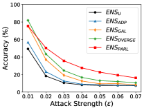
(c) MIM

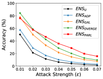
(d) PGD

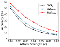
(e) FGSM

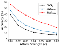
(f) BIM

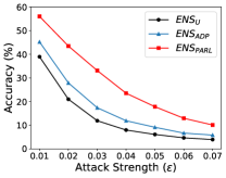
(g) MIM

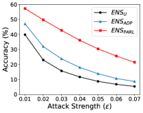
(h) PGD

Figure 3: Ensemble classification accuracy (%) v.s. Attack Strength ($\epsilon$) against different black-box transfer attacks generated from surrogate ensemble for CIFAR-10 [(a), (b), (c), (d)] and CIFAR-100 [(e), (f), (g), (h)] datasets.

Performance in the Presence of $\mathcal{A}_{\mathcal{P}}$: Next, we evaluate the robustness of ensembles when the attacker has complete access to the model parameters. Under such a white-box scenario, we craft adversarial examples from the target ensemble itself. We consider the same attack methodologies and settings as discussed in Section 5.1. We randomly select 1000 test samples and evaluate white-box attacks for all the ensembles across a wide range of attack strength $\epsilon$. We present the results for CIFAR-10 and CIFAR-100 in Figure 4. For CIFAR-10 evaluation (ref. Figure 4a - Figure 4d), we can observe that $ENS_{PARL}$ performs marginally better than the other ensembles. For CIFAR-100 evaluation (ref. Figure 4e - Figure 4h), we can observe that $ENS_{PARL}$ performs better than both $ENS_{\mathcal{U}}$ and $ENS_{ADP}$ for all scenarios. Although PARL achieves the highest robustness among all the previous ensemble methods for black-box transfer attacks, its robustness against white-box attacks is still quite low. The result is expected as the objective of PARL is to increase the diversity of an ensemble against adversarial vulnerability rather than entirely eliminate it. In other words, adversarial vulnerability inevitably exists within the ensemble and can be captured by attacks with white-box access. One straightforward way to improve the robustness of ensembles against such vulnerability is to augment PARL with adversarial training [27], which we look forward to as a future research direction.

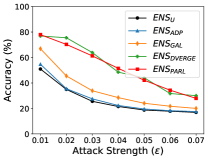
(a) FGSM

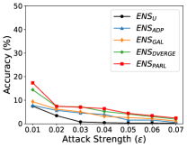
(b) BIM

(c) MIM

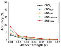
(d) PGD

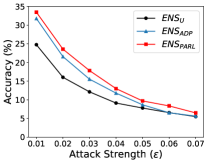
(e) FGSM

(f) BIM

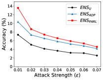
(g) MIM

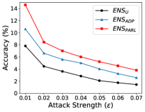
(h) PGD

Figure 4: Ensemble classification accuracy (%) v.s. Attack Strength ($\epsilon$) against different white-box attacks for CIFAR-10 [(a), (b), (c), (d)] and CIFAR-100 [(e), (f), (g), (h)] datasets.

5.4 Ablation Study

In all the previous evaluations, we consider $ENS_{PARL}$ by enforcing diversity in the first seven convolution layers for all the classifiers during ensemble training using PARL. In this section, we provide an ablation study by analyzing a varying number of convolution layers considered for the diversity training. We consider three ensembles $ENS_{PARL/7}$, $ENS_{PARL/5}$, and $ENS_{PARL/3}$ for this study, where $ENS_{PARL/N}$ denotes that the first $N$ convolution layers are used for enforcing the diversity. We consider the same evaluation configurations as discussed in Section 5.1. The accuracies of all the ensembles on clean examples considering both CIFAR-10 and CIFAR-100 are mentioned in Table 2. We can observe that as fewer restrictions are imposed, the overall ensemble accuracy increases, which is expected and can be followed from Equation (1). A detailed analysis on the diversity achieved by all these ensembles in terms of Linear CKA metric is provided in Appendix B for interested readers.

Table 2: Ensemble classification accuracy (%) on the test set for CIFAR-10 and CIFAR-100. The numbers in the first row after slash denote the number of convolution layers used to enforce diversity

	$ENS_{PARL/7}$	$ENS_{PARL/5}$	$ENS_{PARL/3}$
CIFAR-10	91.09	91.18	92.45
CIFAR-100	67.52	67.54	68.81

Next, we evaluate the robustness of these ensembles against black-box transfer attacks for the evaluation configurations discussed in Section 5.1 and provide the results in Figure 5. We can observe that though the ensemble accuracy on clean examples increases with fewer layer restrictions, the robustness against black-box transfer attacks decreases significantly. The results present an interesting trade-off between accuracy and robustness in terms of number of layers considered while computing PARL (ref. Equation (1)).

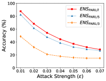
(a) FGSM

(b) BIM

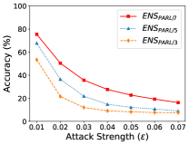
(c) MIM

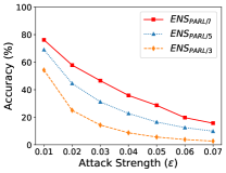
(d) PGD

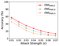
(e) FGSM

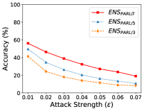
(f) BIM

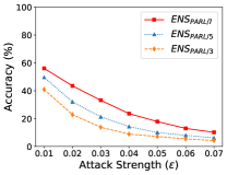
(g) MIM

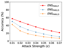
(h) PGD

Figure 5: Ensemble classification accuracy (%) v.s. Attack Strength ($\epsilon$) against different black-box transfer attacks generated from surrogate ensemble for CIFAR-10 [(a), (b), (c), (d)] and CIFAR-100 [(e), (f), (g), (h)] datasets. The numbers in the figure legends after slash denote the number of convolution layers used to enforce diversity

6 Conclusion

In this paper, we propose an approach to enhance the classification robustness of an ensemble against adversarial attacks by developing diversity in the decision boundaries among all the classifiers within the ensemble. The ensemble network is constructed by the proposed Pairwise Adversarially Robust Loss function utilizing the gradients of each layer with respect to input in all the networks simultaneously. The experimental results show that the proposed method can significantly improve the overall robustness of the ensemble against state-of-the-art black-box transfer attacks without substantially impacting the clean example accuracy. Combining the technique with adversarial training and exploring different efficient methods to construct networks with diverse decision boundaries adhering to the principle outlined in the paper can be interesting future research directions.

Appendix A Brief Overview of Adversarial Example Generation

Let us consider a benign data point $x\in\mathbb{R}^{d}$, classified into class $\mathcal{C}_{i}$ by a classifier $\mathcal{M}$. An untargeted adversarial attack tries to add visually imperceptible perturbation $\eta\in\mathbb{R}^{d}$ to $x$ and creates a new data point $x_{adv}=x+\eta$ such that $\mathcal{M}$ misclassifies $x_{adv}$ into another class $\mathcal{C}_{j}$ other than $\mathcal{C}_{i}$. The imperceptibility is enforced by restricting the $l_{\infty}$-norm of the perturbation $\eta$ to be below a threshold $\epsilon$, i.e., $\|\eta\|_{\infty}\leq\epsilon$ [12, 27]. We term $\epsilon$ as the attack strength.

An adversary can craft adversarial examples by considering the loss function of a model, assuming that the adversary has full access to the model parameters. Let $\mathcal{J}(\theta,x,y)$ denote the loss function of the model, where $\theta$, $x$, and $y$ represent the model parameters, benign input, and corresponding label, respectively. The goal of the adversary is to generate adversarial example $x_{adv}$ such that the loss of the model is maximized while ensuring that the magnitude of the perturbation is upper bounded by $\eta$. Hence, $\mathcal{J}(\theta,x_{adv},y)>\mathcal{J}(\theta,x,y)$ adhering to the constraint $\|x_{adv}-x\|_{\infty}\leq\epsilon$. Several methods have been proposed in the literature to solve this constrained optimization problem. We discuss the methods used in the evaluation of our proposed approach.

Fast Gradient Sign Method (FGSM): This attack is proposed by Goodfellow et al. [12]. The adversarial example is crafted using the following equation

$$x_{adv}=x+\epsilon\cdot sign(\nabla_{x}J(\theta,x,y))$$

where $\nabla_{x}J(\theta,x,y)$ denote the gradient of loss with respect to input.

Basic Iterative Method (BIM): This attack is proposed by Kurakin et al. [24]. The adversarial example is crafted iteratively using the following equation

$$x^{(k+1)}=x^{(k)}+clip_{\epsilon}(\alpha\cdot sign(\nabla_{x}J(\theta,x^{(k)},y)))$$

where $x^{(0)}$ is the benign example. If $r$ is the total number of attack iteration, $x_{adv}=x^{(r)}$. The parameter $\alpha$ is a small step size usually chosen as $\epsilon/r$. The function $clip_{\epsilon}(\cdot)$ is used to generate adversarial examples within $\epsilon$-ball of the original image $x^{(0)}$.

Moment Iterative Method (MIM): This attack is proposed by Dong et al. [9], which won the NeurIPS 2017 Adversarial Competition. This attack is a variant of BIM that crafts adversarial examples iteratively using the following equations

$$g^{(k)} =\nabla_{x}J(\theta,x^{(k)},y)$$

$$g^{(k+1)} =\mu\cdot g^{(k)}+\frac{g^{(k)}}{\|g^{(k)}\|_{1}}$$

$$x^{(k+1)} =x^{(k)}+clip_{\epsilon}(\alpha\cdot sign(g^{(k)}))$$

where $\mu$ is termed as the decay factor.

Projected Gradient Sign Method (PGD): This attack is proposed by [27]. This attack is a variant of BIM with same adversarial example generation process except for $x^{(0)}$ is a randomly perturbed image in the $\epsilon$ neighborhood of the original image.

Appendix B Diversity Results for Ablation Study

In this section, we present an analysis on layer-wise CKA values for each pair of classifiers within the ensemble $ENS_{PARL/7}$, $ENS_{PARL/5}$, and $ENS_{PARL/3}$ trained with both CIFAR-10 and CIFAR-100 datasets. The layer-wise CKA values are shown in Figure 6 to demonstrate the effect of PARL on diversity. We can observe a more significant decline in the CKA values at the initial layers for $ENS_{PARL/7}$ as compared to $ENS_{PARL/5}$ and $ENS_{PARL/3}$, which is expected as $ENS_{PARL/7}$ is trained by restricting more convolution layers. We can also observe that each pair of classifiers show more overall diversity in $ENS_{PARL/7}$ than in $ENS_{PARL/5}$ and $ENS_{PARL/3}$. The overall CKA values are mentioned inside braces within the corresponding figure legends.

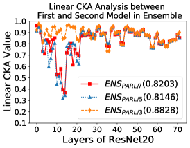
(a)

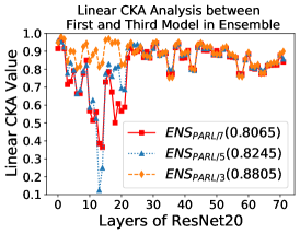
(b)

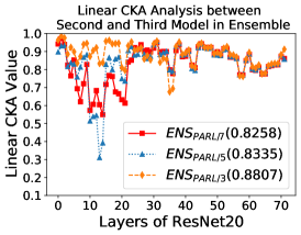
(c)

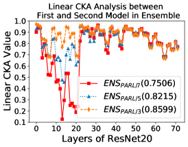
(d)

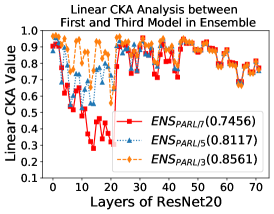
(e)

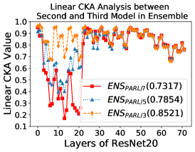
(f)

Figure 6: Layer-wise linear CKA values between each pair of classifiers in $ENS_{PARL/7}$, $ENS_{PARL/5}$, and $ENS_{PARL/3}$ trained with CIFAR-10 [(a), (b), (c)] and CIFAR-100 [(d), (e), (f)] datasets showing the similarities at each layer. The numbers in the figure legends after slash denote the number of convolution layers used to enforce diversity. The value inside the braces within the corresponding figure legends represent the overall average Linear CKA values between each pair of classifiers.

References

- Adam et al. [2018] George-Alexandru Adam, Petr Smirnov, Anna Goldenberg, David Duvenaud, and Benjamin Haibe-Kains. Stochastic combinatorial ensembles for defending against adversarial examples. CoRR, abs/1808.06645, 2018. URL http://arxiv.org/abs/1808.06645.
- Amodei et al. [2016] Dario Amodei et al. Deep speech 2 : End-to-end speech recognition in english and mandarin. In Proceedings of the 33nd International Conference on Machine Learning, ICML 2016, New York City, NY, USA, June 19-24, 2016, volume 48 of JMLR Workshop and Conference Proceedings, pages 173–182. JMLR.org, 2016. URL http://proceedings.mlr.press/v48/amodei16.html.
- Athalye et al. [2018] Anish Athalye, Nicholas Carlini, and David A. Wagner. Obfuscated gradients give a false sense of security: Circumventing defenses to adversarial examples. In Proceedings of the 35th International Conference on Machine Learning, ICML 2018, Stockholmsmässan, Stockholm, Sweden, July 10-15, 2018, volume 80 of Proceedings of Machine Learning Research, pages 274–283. PMLR, 2018. URL http://proceedings.mlr.press/v80/athalye18a.html.
- Bastani et al. [2016] Osbert Bastani, Yani Ioannou, Leonidas Lampropoulos, Dimitrios Vytiniotis, Aditya V. Nori, and Antonio Criminisi. Measuring neural net robustness with constraints. In Advances in Neural Information Processing Systems 29: Annual Conference on Neural Information Processing Systems 2016, December 5-10, 2016, Barcelona, Spain, pages 2613–2621, 2016. URL http://papers.nips.cc/paper/6339-measuring-neural-net-robustness-with-constraints.
- Bhagoji et al. [2017] Arjun Nitin Bhagoji, Daniel Cullina, and Prateek Mittal. Dimensionality reduction as a defense against evasion attacks on machine learning classifiers. CoRR, abs/1704.02654, 2017. URL http://arxiv.org/abs/1704.02654.
- Bojarski et al. [2016] Mariusz Bojarski et al. End to end learning for self-driving cars. CoRR, abs/1604.07316, 2016. URL http://arxiv.org/abs/1604.07316.
- Carlini and Wagner [2017a] Nicholas Carlini and David A. Wagner. Adversarial examples are not easily detected: Bypassing ten detection methods. In Proceedings of the 10th ACM Workshop on Artificial Intelligence and Security, AISec@CCS 2017, Dallas, TX, USA, November 3, 2017, pages 3–14. ACM, 2017a. doi: 10.1145/3128572.3140444. URL https://doi.org/10.1145/3128572.3140444.
- Carlini and Wagner [2017b] Nicholas Carlini and David A. Wagner. Towards evaluating the robustness of neural networks. In 2017 IEEE Symposium on Security and Privacy, SP 2017, San Jose, CA, USA, May 22-26, 2017, pages 39–57. IEEE Computer Society, 2017b. URL https://doi.org/10.1109/SP.2017.49.
- Dong et al. [2018] Yinpeng Dong, Fangzhou Liao, Tianyu Pang, Hang Su, Jun Zhu, Xiaolin Hu, and Jianguo Li. Boosting adversarial attacks with momentum. In 2018 IEEE Conference on Computer Vision and Pattern Recognition, CVPR 2018, Salt Lake City, UT, USA, June 18-22, 2018, pages 9185–9193. Computer Vision Foundation / IEEE Computer Society, 2018. doi: 10.1109/CVPR.2018.00957. URL http://openaccess.thecvf.com/content_cvpr_2018/html/Dong_Boosting_Adversarial_Attacks_CVPR_2018_paper.html.
- Feinman et al. [2017] Reuben Feinman, Ryan R. Curtin, Saurabh Shintre, and Andrew B. Gardner. Detecting adversarial samples from artifacts. CoRR, abs/1703.00410, 2017. URL http://arxiv.org/abs/1703.00410.
- Gong et al. [2017] Zhitao Gong, Wenlu Wang, and Wei-Shinn Ku. Adversarial and clean data are not twins. CoRR, abs/1704.04960, 2017. URL http://arxiv.org/abs/1704.04960.
- Goodfellow et al. [2015] Ian J. Goodfellow, Jonathon Shlens, and Christian Szegedy. Explaining and harnessing adversarial examples. In 3rd International Conference on Learning Representations, ICLR 2015, San Diego, CA, USA, May 7-9, 2015, Conference Track Proceedings, 2015. URL http://arxiv.org/abs/1412.6572.
- Grefenstette et al. [2018] Edward Grefenstette, Robert Stanforth, Brendan O’Donoghue, Jonathan Uesato, Grzegorz Swirszcz, and Pushmeet Kohli. Strength in numbers: Trading-off robustness and computation via adversarially-trained ensembles. CoRR, abs/1811.09300, 2018. URL http://arxiv.org/abs/1811.09300.
- Grosse et al. [2017] Kathrin Grosse, Praveen Manoharan, Nicolas Papernot, Michael Backes, and Patrick D. McDaniel. On the (statistical) detection of adversarial examples. CoRR, abs/1702.06280, 2017. URL http://arxiv.org/abs/1702.06280.
- Gu and Rigazio [2015] Shixiang Gu and Luca Rigazio. Towards deep neural network architectures robust to adversarial examples. In 3rd International Conference on Learning Representations, ICLR 2015, San Diego, CA, USA, May 7-9, 2015, Workshop Track Proceedings, 2015. URL http://arxiv.org/abs/1412.5068.
- He et al. [2016] Kaiming He, Xiangyu Zhang, Shaoqing Ren, and Jian Sun. Deep residual learning for image recognition. In 2016 IEEE Conference on Computer Vision and Pattern Recognition, CVPR 2016, Las Vegas, NV, USA, June 27-30, 2016, pages 770–778. IEEE Computer Society, 2016. doi: 10.1109/CVPR.2016.90. URL https://doi.org/10.1109/CVPR.2016.90.
- Hendrycks and Gimpel [2017] Dan Hendrycks and Kevin Gimpel. Early methods for detecting adversarial images. In 5th International Conference on Learning Representations, ICLR 2017, Toulon, France, April 24-26, 2017, Workshop Track Proceedings. OpenReview.net, 2017. URL https://openreview.net/forum?id=B1dexpDug.
- Huang et al. [2015] Ruitong Huang, Bing Xu, Dale Schuurmans, and Csaba Szepesvári. Learning with a strong adversary. CoRR, abs/1511.03034, 2015. URL http://arxiv.org/abs/1511.03034.
- Jin et al. [2015] Jonghoon Jin, Aysegul Dundar, and Eugenio Culurciello. Robust convolutional neural networks under adversarial noise. CoRR, abs/1511.06306, 2015. URL http://arxiv.org/abs/1511.06306.
- Kariyappa and Qureshi [2019] Sanjay Kariyappa and Moinuddin K. Qureshi. Improving adversarial robustness of ensembles with diversity training. CoRR, abs/1901.09981, 2019. URL http://arxiv.org/abs/1901.09981.
- Kingma and Ba [2015] Diederik P. Kingma and Jimmy Ba. Adam: A method for stochastic optimization. In Yoshua Bengio and Yann LeCun, editors, 3rd International Conference on Learning Representations, ICLR 2015, San Diego, CA, USA, May 7-9, 2015, Conference Track Proceedings, 2015. URL http://arxiv.org/abs/1412.6980.
- Kornblith et al. [2019] Simon Kornblith, Mohammad Norouzi, Honglak Lee, and Geoffrey E. Hinton. Similarity of neural network representations revisited. In Proceedings of the 36th International Conference on Machine Learning, ICML 2019, 9-15 June 2019, Long Beach, California, USA, volume 97 of Proceedings of Machine Learning Research, pages 3519–3529. PMLR, 2019. URL http://proceedings.mlr.press/v97/kornblith19a.html.
- Krizhevsky et al. [2009] Alex Krizhevsky, Geoffrey Hinton, et al. Learning multiple layers of features from tiny images. Technical Report, 2009. URL http://citeseerx.ist.psu.edu/viewdoc/download?doi=10.1.1.222.9220&rep=rep1&type=pdf.
- Kurakin et al. [2017] Alexey Kurakin, Ian J. Goodfellow, and Samy Bengio. Adversarial examples in the physical world. In 5th International Conference on Learning Representations, ICLR 2017, Toulon, France, April 24-26, 2017, Workshop Track Proceedings. OpenReview.net, 2017. URL https://openreview.net/forum?id=HJGU3Rodl.
- Li and Li [2017] Xin Li and Fuxin Li. Adversarial examples detection in deep networks with convolutional filter statistics. In IEEE International Conference on Computer Vision, ICCV 2017, Venice, Italy, October 22-29, 2017, pages 5775–5783. IEEE Computer Society, 2017. doi: 10.1109/ICCV.2017.615. URL https://doi.org/10.1109/ICCV.2017.615.
- Liu et al. [2017] Yanpei Liu, Xinyun Chen, Chang Liu, and Dawn Song. Delving into transferable adversarial examples and black-box attacks. In 5th International Conference on Learning Representations, ICLR 2017, Toulon, France, April 24-26, 2017, Conference Track Proceedings. OpenReview.net, 2017. URL https://openreview.net/forum?id=Sys6GJqxl.
- Madry et al. [2018] Aleksander Madry, Aleksandar Makelov, Ludwig Schmidt, Dimitris Tsipras, and Adrian Vladu. Towards deep learning models resistant to adversarial attacks. In 6th International Conference on Learning Representations, ICLR 2018, Vancouver, BC, Canada, April 30 - May 3, 2018, Conference Track Proceedings. OpenReview.net, 2018. URL https://openreview.net/forum?id=rJzIBfZAb.
- Metzen et al. [2017] Jan Hendrik Metzen, Tim Genewein, Volker Fischer, and Bastian Bischoff. On detecting adversarial perturbations. In 5th International Conference on Learning Representations, ICLR 2017, Toulon, France, April 24-26, 2017, Conference Track Proceedings. OpenReview.net, 2017. URL https://openreview.net/forum?id=SJzCSf9xg.
- Moosavi-Dezfooli et al. [2016] Seyed-Mohsen Moosavi-Dezfooli, Alhussein Fawzi, and Pascal Frossard. Deepfool: A simple and accurate method to fool deep neural networks. In 2016 IEEE Conference on Computer Vision and Pattern Recognition, CVPR 2016, Las Vegas, NV, USA, June 27-30, 2016, pages 2574–2582. IEEE Computer Society, 2016. URL https://doi.org/10.1109/CVPR.2016.282.
- Pang et al. [2019] Tianyu Pang, Kun Xu, Chao Du, Ning Chen, and Jun Zhu. Improving adversarial robustness via promoting ensemble diversity. In Proceedings of the 36th International Conference on Machine Learning, ICML 2019, 9-15 June 2019, Long Beach, California, USA, volume 97 of Proceedings of Machine Learning Research, pages 4970–4979. PMLR, 2019. URL http://proceedings.mlr.press/v97/pang19a.html.
- Papernot et al. [2016] Nicolas Papernot, Patrick D. McDaniel, Xi Wu, Somesh Jha, and Ananthram Swami. Distillation as a defense to adversarial perturbations against deep neural networks. In IEEE Symposium on Security and Privacy, SP 2016, San Jose, CA, USA, May 22-26, 2016, pages 582–597. IEEE Computer Society, 2016. doi: 10.1109/SP.2016.41. URL https://doi.org/10.1109/SP.2016.41.
- Papernot et al. [2017] Nicolas Papernot, Patrick D. McDaniel, Ian J. Goodfellow, Somesh Jha, Z. Berkay Celik, and Ananthram Swami. Practical black-box attacks against machine learning. In Proceedings of the 2017 ACM on Asia Conference on Computer and Communications Security, AsiaCCS 2017, Abu Dhabi, United Arab Emirates, April 2-6, 2017, pages 506–519. ACM, 2017. doi: 10.1145/3052973.3053009. URL https://doi.org/10.1145/3052973.3053009.
- Papernot et al. [2018] Nicolas Papernot, Fartash Faghri, Nicholas Carlini, Ian Goodfellow, Reuben Feinman, Alexey Kurakin, Cihang Xie, Yash Sharma, Tom Brown, Aurko Roy, Alexander Matyasko, Vahid Behzadan, Karen Hambardzumyan, Zhishuai Zhang, Yi-Lin Juang, Zhi Li, Ryan Sheatsley, Abhibhav Garg, Jonathan Uesato, Willi Gierke, Yinpeng Dong, David Berthelot, Paul Hendricks, Jonas Rauber, Rujun Long, and Patrick McDaniel. Technical report on the cleverhans v2.1.0 adversarial examples library. CoRR, abs/1610.00768, 2018. URL https://arxiv.org/abs/1610.00768.
- Rozsa et al. [2016] Andras Rozsa, Ethan M. Rudd, and Terrance E. Boult. Adversarial diversity and hard positive generation. In 2016 IEEE Conference on Computer Vision and Pattern Recognition Workshops, CVPR Workshops 2016, Las Vegas, NV, USA, June 26 - July 1, 2016, pages 410–417. IEEE Computer Society, 2016. doi: 10.1109/CVPRW.2016.58. URL https://doi.org/10.1109/CVPRW.2016.58.
- Shaham et al. [2015] Uri Shaham, Yutaro Yamada, and Sahand Negahban. Understanding adversarial training: Increasing local stability of neural nets through robust optimization. CoRR, abs/1511.05432, 2015. URL http://arxiv.org/abs/1511.05432.
- Strauss et al. [2017] Thilo Strauss, Markus Hanselmann, Andrej Junginger, and Holger Ulmer. Ensemble methods as a defense to adversarial perturbations against deep neural networks. CoRR, abs/1709.03423, 2017. URL http://arxiv.org/abs/1709.03423.
- Szegedy et al. [2014] Christian Szegedy, Wojciech Zaremba, Ilya Sutskever, Joan Bruna, Dumitru Erhan, Ian J. Goodfellow, and Rob Fergus. Intriguing properties of neural networks. In 2nd International Conference on Learning Representations, ICLR 2014, Banff, AB, Canada, April 14-16, 2014, Conference Track Proceedings, 2014. URL http://arxiv.org/abs/1312.6199.
- Szegedy et al. [2016] Christian Szegedy, Vincent Vanhoucke, Sergey Ioffe, Jonathon Shlens, and Zbigniew Wojna. Rethinking the inception architecture for computer vision. In 2016 IEEE Conference on Computer Vision and Pattern Recognition, CVPR 2016, Las Vegas, NV, USA, June 27-30, 2016, pages 2818–2826. IEEE Computer Society, 2016. doi: 10.1109/CVPR.2016.308. URL https://doi.org/10.1109/CVPR.2016.308.
- Tramèr et al. [2018] Florian Tramèr, Alexey Kurakin, Nicolas Papernot, Ian J. Goodfellow, Dan Boneh, and Patrick D. McDaniel. Ensemble adversarial training: Attacks and defenses. In 6th International Conference on Learning Representations, ICLR 2018, Vancouver, BC, Canada, April 30 - May 3, 2018, Conference Track Proceedings. OpenReview.net, 2018. URL https://openreview.net/forum?id=rkZvSe-RZ.
- Wu et al. [2016] Yonghui Wu et al. Google’s neural machine translation system: Bridging the gap between human and machine translation. CoRR, abs/1609.08144, 2016. URL http://arxiv.org/abs/1609.08144.
- Yang et al. [2020] Huanrui Yang, Jingyang Zhang, Hongliang Dong, Nathan Inkawhich, Andrew Gardner, Andrew Touchet, Wesley Wilkes, Heath Berry, and Hai Li. DVERGE: diversifying vulnerabilities for enhanced robust generation of ensembles. In Hugo Larochelle, Marc’Aurelio Ranzato, Raia Hadsell, Maria-Florina Balcan, and Hsuan-Tien Lin, editors, Advances in Neural Information Processing Systems 33: Annual Conference on Neural Information Processing Systems 2020, NeurIPS 2020, December 6-12, 2020, virtual, 2020. URL https://proceedings.neurips.cc/paper/2020/hash/3ad7c2ebb96fcba7cda0cf54a2e802f5-Abstract.html.
- Zheng et al. [2016] Stephan Zheng, Yang Song, Thomas Leung, and Ian J. Goodfellow. Improving the robustness of deep neural networks via stability training. In 2016 IEEE Conference on Computer Vision and Pattern Recognition, CVPR 2016, Las Vegas, NV, USA, June 27-30, 2016, pages 4480–4488. IEEE Computer Society, 2016. doi: 10.1109/CVPR.2016.485. URL https://doi.org/10.1109/CVPR.2016.485.