Freezable bound states in the continuum for time-dependent quantum potentials

Abstract

In this work, we construct time-dependent potentials for the Schrödinger equation via supersymmetric quantum mechanics. The generated potentials have a quantum state with the property that after a particular threshold time $t_{F}$, when the potential does no longer change, the evolving state becomes a bound state in the continuum, its probability distribution freezes. After the factorization of a geometric phase, the state satisfies a stationary Schrödinger equation with time-independent potential. The procedure can be extended to support more than one bound state in the continuum. Closed expressions for the potential, the bound states in the continuum, and scattering states are given for the examples starting from the free particle.

Keywords: Bound states in the continuum, Supersymmetric quantum mechanics

1 Introduction

Bound states in the continuum (BICs) were first discussed in quantum mechanics in the seminal work of von Neumann and Wigner [1], where they construct a localized, normalizable zero-mode state of the form $\psi(r)=\sin(r^{3})/r^{2}$ in the potential $V(r)=2r^{-2}+9r^{4}$, which admits only continuum spectrum solutions for non-vanishing energy eigenvalues. These authors further considered a wave function including modulation of the free particle profile. By analyzing the behavior of the mode as $r\to\infty$ with an energy $E\geq 0$ embedded in the continuum, they construct a periodic potential from the modulated wave function $V(r)=E+\nabla^{2}\psi(r)/\psi(r)$ such that $V(r\to\infty)\sim-|V_{0}|<E$. Upon demanding the normalizability of the state, the potential hence constructed exhibits oscillatory behavior with half the period of the wave function, in such a way that the localization required for the normalization of the state can be understood as the result of its reflection on the Bragg mirror generated by the crests of the oscillation of the potential. The family of von Neumann-Wigner potentials has been continuously revisited for almost a century (see, for instance, Refs. [2, 3, 4]). It is known that potentials of the form $V(r)=a\sin(br)/r$ admit a BIC at energy $E=b^{2}/4$ provided $|a|>|b|$ [5]. These quantum states have been studied under several approaches, including the Gelfan-Levitan equation [6] or inverse scattering approach [4, 7], Darboux transformations [8, 9, 10], supersymmetry (SUSY) [11, 12, 13], among others. Nevertheless, nowadays, BICs are recognized as a general wave phenomenon [14] explored in various scenarios, including atomic physics [3, 15, 16], optic waveguides [17], acoustics [18, 19], and even water waves [20]. Special interest deserves the development of such states in materials, ranging from photonics to quantum dots in a plethora of different setups and aiming for technological applications (see [14] for a review). BICs have also been studied in graphene [21], some topologically insulating materials [22] and, from the formal point of view, modeling the Dirac equation in curved space [23]. A common denominator in these cases is the static character of the effective potential in the effective wave equation governing the underlying system.

Although the completeness of the continuum spectrum of a wave operator might suggest that in principle, any localized squared integrable wave function can be expressed as a combination of these states, in the case of the Schrödinger equation, one has to be careful as far as the realization of BICs is concerned. For instance, in the case of time-dependent potentials, when the time evolution of the potential is frozen, it is not guaranteed that combinations of this kind are automatically solutions to the stationary Schrödinger equation, as we present in this article. The time-dependent Schrödinger equation can be solved exactly in a handful of cases, such as potential wells with moving walls [24, 25, 26]. Several approximations are known to explore the analytical properties of the time-dependent wavefunctions and energy eigenvalues (see, for instance, Ref. [27] and references therein), including the adiabatical approximation [28] and perturbation theory [25]. A powerful strategy to construct time-dependent solutions to the Schrödinger equation from its stationary version is through point transformations [29, 30, 31, 32, 33]. These transformations, in combination with first-order time-independent SUSY, have allowed extending the number of solvable time-dependent examples, from the infinite potential well with a moving wall to the trigonometric Pöschl-Teller potential [26], by transforming the stationary Schrödinger equation to a time-dependent equation that in the remote past/future connects with the solutions of the free particle.

This article presents a general framework for constructing time-dependent potentials for the Schrödinger equation employing second-order supersymmetry in combination with point transformations. We build a BIC for the time-dependent case by point-transforming the stationary problem, modifying the potential and wavefunction. Then, we assume that after a specific time, all the time dependence of the potential is frozen, such that the potential becomes once more stationary and, we explore the behavior of the normalizable state. Intriguingly, it is seen that the freezable BIC is not an eigensolution of the stationary Schrödinger equation in the frozen potential but rather solves an equation that includes a vector potential that does not generate a magnetic field, nevertheless. Thus, by an appropriate gauge transformation, we gauge away the vector potential and observe the BIC that remains frozen when the potential ceases to evolve in time. We exemplify these features starting with the wave function of a free particle in the real positive semi-axis. We further extend this system by constructing a second BIC hence illustrating the procedure to find more intricate systems that support a finite [34, 35] and infinite number [4, 36, 37] of BICs. To this end, we have organized the remaining of this article as follows: In Section 2 we describe the preliminaries of SUSY, point transformations, gauge invariance, and geometric phases in our framework. Section 3 presents the setup for BICs and how to freeze them within the framework. Explicit examples are discussed in Section 4, and final remarks are presented in Section 5.

2 Preliminaries

Before going into the general technique, let us introduce the three main tools we need to generate time-dependent potentials with freezable bound states in the continuum. First, confluent supersymmetric quantum mechanics allows modifying the spectrum of a quantum Hamiltonian. A point transformation provides dynamics into the system. Finally, a gauge transformation facilitates the interpretation of the results.

2.1 Supersymmetric Quantum Mechanics

Supersymmetric Quantum Mechanics or SUSY is a technique that allows us to find solutions of a Schrödinger equation given that we know a solution of another Schrödinger equation with different potential term [38, 39, 40, 41, 42, 43]. In it simplest form, we consider a one dimensional quantum Hamiltonian $H_{0}$ and a first-order differential operator $L_{1}^{\dagger}$ that maps solutions of the eigenvalue equation $H_{0}\psi~{}=~{}E\psi$ into solutions of $H_{1}\hat{\psi}=E\hat{\psi}$, where $H_{1}$ is a Hamiltonian with a deformed potential term. In this work, we consider confluent supersymmetry, which is a second-order SUSY that can be seen as two iterations of first-order transformations [44, 45, 8, 46, 47, 48, 49, 50, 51, 52, 53, 54, 55]. For sake of completeness, let us review the necessary parts of the formalism required for this work. We start out by considering a Hermitian Hamiltonian $H_{0}$ with a time-independent potential $V_{0}(y)$ that could have discrete, continuous spectra, or both. Also, we consider as known some solutions of the eigenvalue equation:

$$H_{0}\psi=E\psi,\quad\text{where}\quad H_{0}=-\frac{d^{2}}{dy^{2}}+V_{0}(y),$$ (1)

$y\in(y_{\ell},y_{r})\subset\mathbb{R}$ and $E$ is the real energy parameter. Then, we apply two very specific steps of 1-SUSY to arrive to a confluen SUSY transformation.

2.1.1 First-order supersymmetry

As a first step, we propose the intertwining relation

$$H_{1}L_{1}^{\dagger}=L_{1}^{\dagger}H_{0},$$ (2)

where

$$H_{1}=-\frac{d^{2}}{dy^{2}}+V_{1}(y),\qquad L_{1}^{\dagger}=-\frac{d}{dy}+\frac{u^{\prime}}{u},$$ (3)

$u=u(y)$ is a function to be found called seed or transformation function. By substituting (3) into the intertwining relation (2) we find that $V_{1}$ and $u$ must fulfill

$$V_{1}(y)=V_{0}(y)-2\frac{d^{2}}{dy^{2}}\ln u,\quad-u^{\prime\prime}+V_{0}u=\epsilon u,$$ (4)

where $\epsilon$ is a real integration constant called factorization energy. Notice that $u$ satisfies the initial Schrödinger equation for the energy parameter $\epsilon$ but we do not impose on it the boundary conditions of the initial physical problem. From expression (4) we see that to have a regular potential $V_{1}$ the transformation function $u$ must not vanish. By applying the operator $L_{1}^{\dagger}$ onto a solution $\psi$ we can obtain eigenfunctions $\hat{\psi}\propto L_{1}^{\dagger}\psi$ of the Hamiltonian $H_{1}$, the intertwining equation (2) guarantees this. In other words, the operator $L_{1}^{\dagger}$ maps the space of solutions of $H_{0}\psi=E\psi$ onto the space of solutions $H_{1}\hat{\psi}=E\hat{\psi}$. An inverse map exists and can be found from the formally adjoint intertwining relation (2), $H_{0}L_{1}=L_{1}H_{1}$, where $L_{1}=(L_{1}^{\dagger})^{\dagger}=d/dy+u^{\prime}/u$. Note that operators $L_{1}$ and $L_{1}^{\dagger}$ factorize the Hamiltonians $H_{0}$ and $H_{1}$ as $L_{1}L_{1}^{\dagger}=H_{0}-\epsilon$, $L_{1}^{\dagger}L_{1}=H_{1}-\epsilon$. Such factorizations are useful to find the missing state of $H_{1}$, it is the state annihilated by $L_{1}$, and it satisfies the equation $H_{1}\hat{\psi}_{\epsilon}=\epsilon\hat{\psi}_{\epsilon}$. By solving the first-order differential equation $L_{1}\hat{\psi}_{\epsilon}=0$ we find that

$$\hat{\psi}_{\epsilon}(y)=\hat{c}_{\epsilon}\frac{1}{u(y)},$$ (5)

where $\hat{c}_{\epsilon}$ is a normalization constant when $\hat{\psi}_{\epsilon}$ is normalizable, otherwise $\hat{c}_{\epsilon}=1$. Now, any other solution of $H_{1}\hat{\psi}=E\hat{\psi}$ besides $\hat{\psi}_{\epsilon}$ can be obtained as $\hat{\psi}\propto L_{1}^{\dagger}\psi$. Because we know that $L_{1}L_{1}^{\dagger}=H_{0}-\epsilon$, we can calculate the normalization constant. Assuming $\left\lVert\psi\right\rVert^{2}=1$, we see that

$$\hat{\psi}=\frac{1}{\sqrt{E-\epsilon}}L_{1}^{\dagger}\psi.$$ (6)

Thus, starting from a Schrödinger equation $H_{0}\psi=E\psi$ with potential $V_{0}$, and solutions $\psi$, we obtain a Schrodinger equation $H_{1}\hat{\psi}=E\hat{\psi}$ with a potential $V_{1}$, and solutions $\hat{\psi}_{\epsilon}$ and $\hat{\psi}$, see (4), (5) and (6).

2.1.2 Second-order confluent supersymmetry

We can iterate the procedure and obtain a second Hamiltonian $H_{2}$. The selection of the transformation function $v$ and the factorization energy $\varepsilon$ by properly solving $H_{1}v=\varepsilon v$, will fix $H_{2}$ and consequently its eigenfunctions. There exist many variations of the second iteration leading to different systems. The most common is when $\epsilon\neq\varepsilon$ are taken both as real constants. Here we consider the case $\epsilon=\varepsilon\in\mathbb{R}$ . Once we fixed the factorization constant, we need to select a transformation function $v$. A reasonable choice is the missing state $v=1/u$, but this choice results in $H_{2}=H_{0}$. Since we want to generate a Hamiltonian different from the initial one, $H_{2}\neq H_{0}$, we need to use a general solution of $H_{1}v=\epsilon v$; this can be done using the reduction of order formula,

$$v=\frac{1}{u}\left(\omega+\int^{y}_{y_{0}}u^{2}(z)dz\right),$$ (7)

where $\omega$ is a real constant. The potential associated to this second iteration becomes

$$V_{2}(y)=V_{1}(y)-2\frac{d^{2}}{dy^{2}}\ln v=V_{0}(y)-2\frac{d^{2}}{dy^{2}}\ln\left(\omega+\int^{y}_{y_{0}}u^{2}dz\right).$$ (8)

The Hamiltonians $H_{0}$ and $H_{2}$ are intertwined by the operator

$$L^{\dagger}=L_{2}^{\dagger}L_{1}^{\dagger}=\left(-\frac{d}{dy}+\frac{v^{\prime}}{v}\right)\left(-\frac{d}{dy}+\frac{u^{\prime}}{u}\right),$$ (9)

as $H_{2}L^{\dagger}=L^{\dagger}H_{0}$.

Solutions of the equation $H_{2}\bar{\psi}=E\bar{\psi}$ can be found applying $L^{\dagger}$ onto solutions of $H_{0}\psi=E\psi$ as

$$\bar{\psi}=\frac{1}{E-\epsilon}L^{\dagger}\psi.$$ (10)

Moreover, the associated missing state to the factorization energy $\epsilon$ is

$$\bar{\psi}_{\epsilon}=C_{\epsilon}\frac{1}{v}=C_{\epsilon}\frac{u}{\omega+\int^{y}_{y_{0}}u^{2}dz},$$ (11)

where $C_{\epsilon}$ is a normalization constant, if $\bar{\psi}_{\epsilon}$ is square integrable. In the first-order SUSY, the transformation function $u$ must be nodeless to produce a regular potential $V_{1}$. In the confluent case this restriction changes, the function $\omega+\int_{y_{0}}^{y}u^{2}dz$ must not vanish. We can fulfill this requirement selecting $u$ such that either $\lim_{y\to y_{\ell}}u(y)=0$ or $\lim_{y\to y_{r}}u(y)=0$, then we can guarantee that there exist constants $\omega$ and $y_{0}$ that keep $V_{2}$ regular.

2.2 Point transformation

We can relate a one-dimensional time-independent Schrödinger equation with a time-dependent one using a point transformation, see for example [29, 30]. Moreover, the connection between a time-dependent Supersymmetry presented in [38, 56] and the time-independent version was done in [57]. The combination of Supersymmetric QM and point transformations was further exploited in [58, 59, 60, 61, 26]. In particular, let us consider the time-independent Schrödinger equation of the SUSY partner potential $V_{2}(y)$:

$$\frac{d^{2}}{dy^{2}}\bar{\psi}(y)+(E-V_{2}(y))\bar{\psi}(y)=0.$$ (12)

Now, let us consider arbitrary functions $A=A(t)$ and $B=B(t)$ and let the variable $y$ be defined in terms of a temporal parameter $t$ and a new spatial variable $x$ as:

$$y(x,t)=x\exp\left[4\int_{t_{0}}^{t}A(\tau)d\tau\right]+2\int_{t_{0}}^{t}B(\tau)\exp\left[4\int_{\tau_{0}}^{\tau}A(\tilde{\tau})d\tilde{\tau}\right]d\tau,$$ (13)

then the function

$$\phi(x,t) = \hat{\psi}(y(x,t))\exp\left\{-i\left[A(t)x^{2}+B(t)x+E\int_{t_{0}}^{t}\exp\left[8\int_{\tau_{0}}^{\tau}A(\tilde{\tau})d\tilde{\tau}\right]d\tau\right.\right.$$ (14)

$$\left.\left.+\int_{t_{0}}^{t}\left[2iA(\tau)+B^{2}(\tau)\right]d\tau\right]\right\},$$

is solution of the equation

$$i\frac{\partial}{\partial t}\phi(x,t)+\frac{\partial^{2}}{\partial x^{2}}\phi(x,t)-V(x,t)\phi(x,t)=0.$$ (15)

The former is a time-dependent Schrödinger equation (TDSE) where the potential is given by

$$V(x,t) = \exp\left[8\int_{t_{0}}^{t}A(\tau)d\tau\right]V_{2}(y(x,t))+\left[\frac{d}{dt}A(t)-4A^{2}(t)\right]x^{2}$$ (16)

$$+\left[\frac{d}{dt}B(t)-4A(t)B(t)\right]x.$$

In the last expression we have three terms. The first one involves the potential $V_{2}$ in terms of $x,~{}t$ with a time-dependent coefficient. The last two terms are a quadratic and linear monomials in the $x$ coordinate with time-dependent coefficients. Let us set those two last terms equal to zero with the goal to obtain a potential $V$ with a shape similar to the potential $V_{2}$. This problem was studied in [26]. Setting such coefficients to zero we obtain a system of equations; its solution by direct integration is:

$$A(t)=-\frac{1}{4t+c_{1}},\qquad B(t)=\frac{c_{2}}{4t+c_{1}},$$ (17)

where $c_{1}$ and $c_{2}$ are real constants. Once these two functions are known, the change of variable defined in (13) can be evaluated,

$$y(x,t)=\frac{2x-c_{2}}{2(4t+c_{1})}.$$ (18)

Thus, given the stationary Schrödinger equation $\bar{\psi}^{\prime\prime}+(E-V_{2}(y))\bar{\psi}=0$ we can find a solution of the time dependent Schrödinger equation $i\partial_{t}\phi+\partial_{xx}\phi-V\phi=0$ where

$$\phi(x,t)=\frac{1}{\sqrt{4t+c_{1}}}~{}\bar{\psi}\left(\frac{2x+c_{2}}{2(4t+c_{1})}\right)\exp\left\{\frac{i}{4t+c_{1}}\left[x^{2}-c_{2}x+\frac{E+c_{2}^{2}}{4}\right]\right\},$$ (19)

and

$$V(x,t)=\frac{1}{(4t+c_{1})^{2}}V_{2}\left(\frac{2x+c_{2}}{2(4t+c_{1})}\right).$$ (20)

There is a singularity we must avoid at $t=-c_{1}/4$, thus the time domain cannot be whole real line. The domain of the $x$ coordinate could be the same of the $y$ variable, depending on the physical system.

2.3 Gauge invariance and geometric phase

The Schrödinger equation for a particle with charge $q$ in an electromagnetic potential is written in terms of the scalar $\varphi$ and vector potential $\mathbf{A}$ rather than in terms of the electric $\mathbf{E}$ and magnetic $\mathbf{B}$ fields by writing the Hamiltonian as $H=(\hat{\mathbf{p}}+q\mathbf{A})^{2}+q\varphi$. Gauge invariance of Maxwell equations implies that the electric and magnetic fields

$$\mathbf{E}=-\nabla\varphi-\frac{\partial\mathbf{A}}{\partial t},\qquad\mathbf{B}=\nabla\times\mathbf{A}$$ (21)

do not change if the following transformations are performed simultaneously,

$$\mathbf{A}\to\mathbf{A}^{\prime}=\mathbf{A}+\nabla\lambda,\qquad\varphi\to\varphi^{\prime}=\varphi-\frac{\partial\lambda}{\partial t},$$ (22)

where $\lambda=\lambda(x,t)$ is a scalar function. The time-dependent Schrödinger equation $i\partial_{t}\psi=H\psi$ retains this feature if besides the transformations in Eq. (22), the wave function changes according to $\psi\to\psi^{\prime}=e^{i\lambda}\psi$. This allows selecting $\lambda$ in such a way that if at a certain instant of time $t_{F}$ the vector potential $\mathbf{A}\neq 0$ but before we had $\mathbf{A}=0$, one can still have a Schrödinger equation without vector potential by tuning the scalar potential appropriately. In particular, by selecting $\lambda(x,t)=g(x)\Theta(t-t_{F})$, we can shift the scalar potential in such a way that the time-dependent equation governing this state never develops a vector potential.

Furthermore, in the situation where the time-dependent Schrödinger equation

$$i\frac{\partial\psi^{\prime}}{\partial t}=(\hat{\mathbf{p}}+q\mathbf{A})^{2}\psi^{\prime}+q\varphi\psi^{\prime}$$ (23)

involves a vector potential $\mathbf{A}$ such that $\nabla\times\mathbf{A}=0$, we can directly factorize a geometric phase $\psi^{\prime}=e^{ig}\psi$ with

$$g=q\int\mathbf{A}\cdot d\mathbf{x},$$ (24)

where $g$ does not depend on the path of integration in the region where the curl of $\mathbf{A}$ vanishes, in such a way that the function $\psi$ verifies

$$i\frac{\partial\psi}{\partial t}=\hat{\mathbf{p}}^{2}\psi+q\varphi\psi,$$ (25)

namely, a time-dependent Schrödinger equation without vector potential.

3 Freezable bound states in the continuum

Our goal is to construct a solvable time dependent potential. This potential will change in time until a stopping or freezing time $t_{F}$, then it will no longer vary in time:

$$V_{F}(x,t)=\begin{cases}V(x,t)&0\leq t<t_{F},\\ V(x,t_{F})&t\geq t_{F}.\end{cases}$$ (26)

We ask this potential to have at least one BIC when $t\geq t_{F}$, we call these states freezable bound states in the continuum.

We start out from a solvable and stationary potential $V_{0}(y)$ with continuum spectrum. Then, the first step is to construct its confluent SUSY partner $V_{2}(y)$ using the algorithm presented in Section 2.1.2. The factorization energy $\epsilon$ must be in the continuum spectrum of $H_{0}$. As a consequence, the seed solution is a non-normalizable function. Let us study first the case when the domain of the potential is the whole real line. For this case $V_{0}(y)$ must be a bounded potential. Moreover, we ask

$$\lim_{y\rightarrow-\infty}V_{0}(y)=V_{\ell},\quad\lim_{y\rightarrow\infty}V_{0}(y)=V_{r},\qquad V_{\ell}\neq V_{r}.$$ (27)

Without loss of generality, we will consider $V_{\ell}>V_{r}$. Other requirements that we impose to $V_{0}(y)$ are:

$$\int_{y_{a}}^{\infty}|V_{0}^{\prime}|^{2}dy<\infty,\quad\int_{y_{a}}^{\infty}|V_{0}^{\prime\prime}|dy<\infty,\quad\int^{y_{b}}_{-\infty}|V_{0}^{\prime}|^{2}dy<\infty,\quad\int^{y_{b}}_{-\infty}|V_{0}^{\prime\prime}|dy<\infty,$$ (28)

where $y_{a},~{}y_{b}$ are constants with absolute value arbitrarily large.

Since the asymptotic behaviour of the solutions of the Schrödinger equation are important, let us review some general results that will be used. It is known (see, e.g. Theorem 4.6, p.84 in [62]), that the solutions of the equation $-\psi^{\prime\prime}+v_{0}\psi=k^{2}\psi$, for a function $v_{0}(y)$ satisfying $v_{0}\rightarrow 0$ as $y\rightarrow\infty$ and

$$\int_{y_{a}}^{\infty}|v_{0}^{\prime}|^{2}dy<\infty,\quad\int_{y_{a}}^{\infty}|v_{0}^{\prime\prime}|dy<\infty,$$ (29)

have the following asymptotic form as $y\rightarrow\infty$:

$$\psi^{+}(y)=\exp\left(ik\int_{y_{a}}^{y}\sqrt{1-\frac{v_{0}(z)}{k^{2}}}dz\right)\left(1+o(1)\right),$$

$$\phi^{+}(y)=\exp\left(-ik\int_{y_{a}}^{y}\sqrt{1-\frac{v_{0}(z)}{k^{2}}}dz\right)\left(1+o(1)\right).$$ (30)

Since the substitution of $y$ by $-y$ changes neither the form of the conditions (29) nor the equation, then the solution behaves asymptotically when $y\rightarrow-\infty$ as

$$\psi^{-}(y)=\exp\left(ik\int^{y_{b}}_{y}\sqrt{1-\frac{v_{0}(z)}{k^{2}}}dz\right)\left(1+o(1)\right),$$

$$\phi^{-}(y)=\exp\left(-ik\int^{y_{b}}_{y}\sqrt{1-\frac{v_{0}(z)}{k^{2}}}dz\right)\left(1+o(1)\right).$$ (31)

The next consideration is to select a factorization energy $V_{\ell}>\epsilon>V_{r}$. To apply the results (3) we identify $v_{0}=V_{0}-V_{r}$ when analysing the asymptotic at $y\rightarrow\infty$, then

$$\psi^{+}(y)\propto\exp\left(i\sqrt{\epsilon-V_{r}}~{}y\right)\left(1+o(1)\right),\quad\phi^{+}(y)\propto\exp\left(-i\sqrt{\epsilon-V_{r}}~{}y\right)\left(1+o(1)\right),$$ (32)

i.e., we will have only oscillatory solutions. We must select a seed function $u$ as a superposition, such that $u$ is a real function. We can write $u\propto\sin\left(\sqrt{V_{\ell}-\epsilon}~{}y+\delta\right)$, where $\delta$ is a phase. When studying the asymptotic behavior of $u$ at $y\rightarrow-\infty$, we can use $v_{0}=V_{0}-V_{\ell}$. From (3), the solutions of the Schrödinger equation have the form

$$\psi^{-}(y)\propto\exp\left(\sqrt{V_{\ell}-\epsilon}~{}y\right)\left(1+o(1)\right),\quad\phi^{-}(y)\propto\exp\left(-\sqrt{V_{\ell}-\epsilon}~{}y\right)\left(1+o(1)\right),$$ (33)

the possible behaviour of $u$ is a superposition of a divergent and a convergent exponential functions. We must choose only the convergent solution, $u\propto\psi^{-}(y)$. By choosing $u$ with these behaviours as $|y|\rightarrow\infty$, we guarantee that there are ranges for the parameters $y_{0}$ and $\omega$ in (8) where $V_{2}$ is a regular potential.

Moreover, when $y\rightarrow\infty$ then

$$V_{2}\sim V_{0}+2\left\{\frac{2k\sin(2(ky+\delta))}{\frac{\sin(2(ky+\delta))}{2k}+y+\omega_{a}}+\frac{\left[\cos(2(ky+\delta))+1\right]^{2}}{\left[\frac{\sin(2(ky+\delta))}{2k}+y+\omega_{a}\right]^{2}}\right\}\rightarrow V_{r},$$ (34)

where $k^{2}=\epsilon-V_{r}$, and $\omega_{a}$ is a constant. The missing state behaves as

$$\bar{\psi}_{\epsilon}\sim\frac{\sin(ky+\delta)}{\frac{\sin(2(ky+\delta))}{2k}+y+\omega_{1}}\rightarrow 0.$$ (35)

When $y\rightarrow-\infty$ the potential and the missing states behave as

$$V_{2}\sim V_{0}-\frac{16\kappa^{3}\omega_{b}e^{2\kappa y}}{\left(e^{2\kappa y}+2\kappa\omega_{b}\right)^{2}}\rightarrow V_{\ell},\quad\text{and}\quad\bar{\psi}_{\epsilon}\sim\frac{e^{\kappa y}}{\frac{e^{2\kappa y}}{2k}+\omega_{b}}\rightarrow 0,$$ (36)

where $\kappa^{2}=V_{\ell}-\epsilon$. Thus, the potentials $V_{0}$ and $V_{2}$ have the same limit as $y\rightarrow\pm\infty$. Moreover, these results suggest that the function $\bar{\psi}_{\epsilon}$ is square integrable solution of $H_{2}\bar{\psi}_{\epsilon}=\epsilon\bar{\psi}_{\epsilon}$ with an eigenvalue embedded in the continuum spectrum, in other words, it could be a BIC. Such situations have being discussed in [11].

If we start from a potential $V_{0}(y)$ defined in the semiaxis $(0,\infty)$, the potential can be either bounded or unbounded, but we still require $V_{0}(y)\rightarrow V_{r}$ as $y\rightarrow\infty$. Moreover, $V_{0}(y)$ must satisfy the first two conditions in (28). Then, the correct choice of factorization energy is $\epsilon>V_{r}$, as part of the continuum spectrum. The behavior of $u$ when $y\rightarrow\infty$ is oscillatory, as explained in (32). Again, it is necessary to choose a real solution. The behavior of $u$ on the left must be chosen so $u$ does not diverge. In fact, $\lim_{y\rightarrow 0}u(y)=0$ is needed, so the missing state $\bar{\psi}_{\epsilon}$ could satisfy the physical boundary conditions $\bar{\psi}_{\epsilon}(0)=0$.

Now, we can associate to $V_{2}(y)$ a time-dependent potential $V(x,t)$ via the point transformation defined in Section 2.2. In equation (19) we can see how any solution of $H_{2}\bar{\psi}=E\bar{\psi}$ transforms. Recall that solutions $\bar{\psi}$ are obtained from solutions of $H_{0}\psi=E\psi$ as in (10), $\psi$ could be either a bound or a scattering state. There is also a BIC $\bar{\psi}_{\epsilon}$ introduced by the confluent SUSY transformation that also transforms as in (19); it will be called $\phi_{\epsilon}(x,t)$. This function solves the time-dependent Schrödinger equation $i\partial_{t}\phi_{\epsilon}+\partial_{xx}\phi_{\epsilon}-V\phi_{\epsilon}=0$ and will be square integrable. Square integrability of $\phi(x,t)$ is guaranteed if the preimage $\bar{\psi}(y)$ is also a square integrable function,

$$||\phi||^{2}=\int_{-\infty}^{\infty}|\phi(x)|^{2}dx=\frac{1}{4t+c_{1}}\int_{-\infty}^{\infty}\Bigg{|}\bar{\psi}\left(\frac{2x+c_{2}}{2(4t+c_{1})}\right)\Bigg{|}^{2}dx=\int_{-\infty}^{\infty}\big{|}\bar{\psi}(y)\big{|}^{2}dy=||\bar{\psi}||^{2},$$ (37)

where we used the change of variable (18). Neither $\phi(x,t)$ nor $\phi_{\epsilon}(x,t)$ are stationary states, they evolve in time, and they are not eigenfuncions of the operator $-\partial_{xx}+V$.

Our next step is to select a freezing time $t_{F}$. At any time $t\geq t_{F}$, the functions $\phi(x,t_{F})$ and $\phi_{\epsilon}(x,t_{F})$ satisfy the eigenvalue equation:

$$\left[\left(-i\frac{\partial}{\partial x}+A_{x}(x)\right)^{2}+V(x,t_{F})\right]\phi(x,t_{F})=\frac{E}{(4t_{F}+c_{1})^{2}}\phi(x,t_{F}),$$ (38)

where $A_{x}(x)=-\partial_{x}g(x)=-(2x-c_{2})/(4t_{F}+c_{1})$ and

$$g(x)=\frac{1}{4t_{F}+c_{1}}\left(x^{2}-c_{2}x+\frac{E+c_{2}^{2}}{4}\right)$$ (39)

is the phase accompanying the wavefunctions (19). Equation (38) is the Schrödinger equation of a charged particle in a magnetic field with vector potential $\mathbf{A}=(A_{x},0,0)$, but a null magnetic field since $\mathbf{B}=\nabla\times\mathbf{A}=0$. Here use the gauge transformation introduced in Section 2.3, that allows introducing a vector potential $\mathbf{A}(x,t)=(A_{x}(x,t),0,0)$ where $A_{x}(x,t)=-\Theta(t-t_{F})\partial_{x}g(x)$, then the piecewise function

$$\phi_{F}(x,t)=\begin{cases}\phi(x,t)&0\leq t<t_{F},\\ \bar{\psi}\left(\frac{2x+c_{2}}{2(4t_{F}+c_{1})}\right)\exp\left(-\frac{iE}{(4t_{F}+c_{1})^{2}}t\right)&t\geq t_{F}.\end{cases}$$ (40)

will be solution of

$$i\partial_{t}\phi_{F}(x,t)=\left[-\partial_{xx}+V_{F}(x,t)\right]\phi_{F}(x,t)=H\phi_{F}(x,t).$$

In particular, the function

$$\phi_{F\epsilon}(x,t)=\begin{cases}\phi_{\epsilon}(x,t)&0\leq t<t_{F},\\ \bar{\psi}_{\epsilon}\left(\frac{2x+c_{2}}{2(4t_{F}+c_{1})}\right)\exp\left(-\frac{i\epsilon}{(4t_{F}+c_{1})^{2}}t\right)&t\geq t_{F},\end{cases}$$ (41)

is a time-dependent wave packet before the freezing time, but after $t_{F}$, it will become a bound state in the continuum satisfying the eigenvalue equation $H\phi_{F\epsilon}=\varepsilon\phi_{F\epsilon}$, where $\varepsilon=\epsilon/(4t_{F}+c_{1})^{2}$.

4 Examples

In this section, we construct two potentials with freezable bound states in the continuum. In the first example, we start from the Free Particle defined in the semiaxis and generate a time-dependent potential with a single freezable BIC. For a second example, we show that we can iterate the algorithm to construct a potential with two freezable BICs. Moreover, using the time-reversal symmetry, we build more potentials with freezable BICS.

4.1 Adding a single freezable bound state in the continuum to the Free-Particle

Let us commence our discussion by considering the Free-Particle potential $V_{0}(y)=0$ defined in the positive semi-axis $y\in(0,\infty)$. We choose a factorization energy $\epsilon=k^{2}>0$ and $u(y)=\sin(ky)$. By using a confluent supersymmetric transformation, the potential $V_{0}$ transform as in (8). Explicitly,

$$V_{2}(y)=\frac{16k^{2}\left[1-k(2\omega+y)\sin(2ky)-\cos(2ky)\right]}{\left[\sin(2ky)-2k(2\omega+y)\right]^{2}}.$$ (42)

To have a regular potential we use $y_{0}=0$ and $\omega>0$. The missing state (11) associated to the factorization energy $\epsilon$ reads

$$\bar{\psi}_{\epsilon}(y)=C_{\epsilon}~{}\frac{4k\sin(ky)}{2k(2\omega+y)-\sin(2ky)},$$ (43)

and it is square integrable. To verify this statement, let us focus on the oscillating tail of the function. We can see that the square of the missing state is bounded from above by a square integrable function from $y=\pi/4k$ to $y\rightarrow\infty$, as follows:

$$||\bar{\psi}_{\epsilon}||^{2} =|C_{\epsilon}|^{2}\left(\int^{\frac{\pi}{4k}}_{0}\left|\bar{\psi}_{\epsilon}(y)\right|^{2}dy+\int_{\frac{\pi}{4k}}^{\infty}\left|\bar{\psi}_{\epsilon}(y)\right|^{2}dy\right)$$

$$=|C_{\epsilon}|^{2}\left(\frac{\pi-2}{\omega(8k\omega+\pi-2)}+\int_{\frac{\pi}{4k}}^{\infty}\left|\frac{4k\sin(ky)}{2k(2\omega+y)-\sin(2ky)}\right|^{2}dy\right)$$

$$\leq|C_{\epsilon}|^{2}\left(\frac{\pi-2}{\omega(8k\omega+\pi-2)}+\int_{\frac{\pi}{4k}}^{\infty}\left|\frac{4k}{2k(2\omega+y)-1}\right|^{2}dy\right)$$

$$=|C_{\epsilon}|^{2}\left(\frac{1}{\omega}+\frac{8k}{8k\omega+\pi-2}\right).$$ (44)

For an energy $E_{q}=q^{2}\neq\epsilon$, the wavefunction $\bar{\psi}(y)$, see (10), is

$$\bar{\psi}(y)=\frac{4k\sin^{2}(ky)\left[k\cot(ky)\sin(qy)-q\cos(qy)\right]}{\left(q^{2}-k^{2}\right)\left[2k(2\omega+y)-\sin(2ky)\right]}-\sin(qy).$$ (45)

In Fig. 1 the potential $V_{2}(y)$, along with the probability densities of the missing state $\bar{\psi}_{\epsilon}(y)$ and a scattering state $\bar{\psi}(y)$ are shown, for $\omega=1$. We observe that the wavefunction of the BIC has an envelop function that goes to zero as $y\to\infty$, whereas the state $\bar{\psi}(y)$ is not localized.

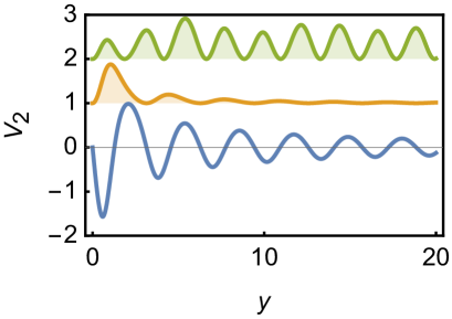
Figure 1: Confluent SUSY partner potential $V_{2}(y)$ of the free particle (blue curve) and probability densities $|\bar{\psi}_{\epsilon}(y)|^{2}$ (orange) and $|\bar{\psi}(y)|^{2}$ (green) for parameters $\omega=1$, $\epsilon=1$ and $q^{2}=2$.

Next, we use the point transformation presented in (18–20), where we set $c_{1}=1,~{}c_{2}=0$ and $t\in[0,\infty)$. This selection makes $x=y$ at $t=0$. Then $y=x/(4t+1)$ and $V_{2}$ transforms as:

$$V(x,t)=\frac{16k^{2}\left[1-k\left(2\omega+\frac{x}{4t+1}\right)\sin\left(\frac{2kx}{4t+1}\right)-\cos\left(\frac{2kx}{4t+1}\right)\right]}{\left[(4t+1)\sin\left(\frac{2kx}{4t+1}\right)-2k(2\omega+8\omega t+x)\right]^{2}}.$$ (46)

Analogously, for the time-dependent BIC, the associated wavefunction for energy $\epsilon$ is explicitly

$$\phi_{\epsilon}(x,t)=\frac{4ik\sqrt{4t+1}\exp\Big{[}{\frac{i\left(4x^{2}+k^{2}\right)}{16t+4}}\Big{]}\sin\left(\frac{kx}{4t+1}\right)}{(4t+1)\sin\left(\frac{2kx}{4t+1}\right)-2k(2\omega+8\omega t+x)}.$$ (47)

The state is localized and the first maximum in the probability density broadens and diminishes in height as time increases. For states with energy $E=q^{2}\neq\epsilon$, the corresponding time-dependent wavefunction has the explicit form

$$\phi(x,t)=\frac{\exp\Big{[}{\frac{i\left(4x^{2}+q^{2}\right)}{16t+4}}\Big{]}}{i\sqrt{4t+1}}\left[\chi_{q}(x,t)-\sin\left(\frac{qx}{4t+1}\right)\right],$$ (48)

where

$$\chi_{q}(x,t)=\frac{4k\sin^{2}\left(\frac{kx}{4t+1}\right)\left[k\cot\left(\frac{kx}{4t+1}\right)\sin\left(\frac{qx}{4t+1}\right)-q\cos\left(\frac{qx}{4t+1}\right)\right]}{(q^{2}-k^{2})\left[4k\omega+\frac{2kx}{4t+1}-\sin\left(\frac{2kx}{4t+1}\right)\right]}.$$

This state is unlocalized at any time.

Finally, we consider a charged particle in the potential:

$$V_{F}(x,t)=\begin{cases}V(x,t)&0\leq t<t_{F},\\ V(x,t_{F})&t\geq t_{F}.\end{cases}$$ (49)

where $V(x,t)$ is given by (46), and $t_{F}$ is the freezing time. The form of the potential at $t=0$ is oscillatory in the whole domain $x\in(0,\infty)$, the amplitude of such oscillations decrease as $1/x$. This potential is in fact a family parametrized by $\omega>0$. The smaller the value of $\omega$ the deeper the first minimum of the potential. The solutions of the time dependent Schrödinger equation $i\partial_{t}\phi_{F}+\partial_{xx}\phi_{F}+V_{F}\phi_{F}=0$ can be constructed as in (40), (45) and (48), these states are non-normalizable. Moreover, the state $\phi_{F\epsilon}$ ends as a bound state in the continuum. It is constructed as in (41) where $\bar{\psi}_{\epsilon}$ is given in (43) and $\phi_{\epsilon}$ in (47). It is square integrable for all times $t\geq 0$ because of relations (37) and (4.1). When $t\geq t_{F}$, the state $\phi_{F\epsilon}$ becomes the only stationary bound state of the Hamiltonian $H_{F}=-\partial_{xx}+V_{F}$ with energy $\epsilon_{F}=\epsilon/(4t+1)^{2}$. Since $\epsilon_{F}>V(x,t_{F})$ when $x\to\infty$, then $\phi_{F\epsilon}$ is a freezable bound state in the continuum. In Fig. 2(a), we show the potential $V_{F}(x,t)$. Its shape changes in time and its spatial profile oscillates as expected, vanishing as $x\to\infty$. Fig. 2(b) shows the probability density of the added freezable BIC, $|\phi_{F\epsilon}(x,t)|^{2}$, it can be seen how it varies in time until $t_{F}=0.2$, when it becomes stationary. The behavior of $|\phi_{F}(x,t)|^{2}$, for $E=2$ at different times is shown in Fig. 2(c).

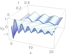
(a)

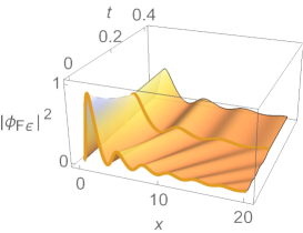
(b)

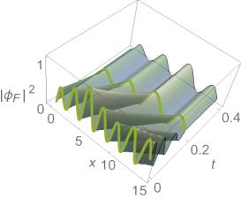
(c)

Figure 2: System with a single freezable BIC. The potential $V_{F}(x,t)$ (a) and probability densities of $\phi_{F\epsilon}(x,t)$ (b) and $\phi_{F}(x,t)$ (c). Here $\omega=1$, $\epsilon=1$, $q^{2}=2$, and $t_{F}=0.2$.

4.2 System with two freezable bound states in the continuum

We can iterate the confluent SUSY transformation to add more than one bound states in the continuum. With every iteration the length of the expressions of the SUSY partner potential and the solutions of the corresponding Schrödinger equation could dramatically increase. To illustrate the procedure, we take the stationary system found in the previous example with the potential term $V_{2}(y)$ as in (42), the single BIC $\bar{\psi}_{\epsilon}(y)$ with energy $\epsilon=k^{2}$ as in (43), and scattering states $\bar{\psi}(y)$ with energy $E_{q}=q^{2}\neq k^{2}$ given by (45). To simplify notation, let us make the following replacements $\epsilon\rightarrow\epsilon_{1},~{}k\rightarrow k_{1}$ and $\omega\rightarrow\omega_{1}$. Next, we find a confluent-SUSY partner of $V_{2}$. Since we want add a second BIC, we need to select a second factorization energy $\epsilon_{2}=k_{2}^{2}\neq\epsilon_{1}$. The seed solution of this transformation will be the scattering state associated to $\epsilon_{2}$:

$$u_{2}(y)=\frac{L_{2}^{+}L_{1}^{+}\bar{\psi}(y)}{k_{2}^{2}-k_{1}^{2}}=\frac{4k_{1}\sin^{2}(k_{1}y)\left[k_{1}\cot(k_{1}y)\sin(k_{2}y)-k_{2}\cos(k_{2}y)\right]}{\left(k_{2}^{2}-k_{1}^{2}\right)\left[2k_{1}(2\omega_{1}+y)-\sin(2k_{1}y)\right]}-\sin(k_{2}y).$$ (50)

From (8), we can see that the SUSY partner potential of $V_{2}$ becomes

$$V_{4}(y)=V_{2}(y)-2\frac{d^{2}}{dy^{2}}\left(\omega_{2}+\int^{y}_{0}u_{2}^{2}dz\right).$$ (51)

The integral in the previous expression can be calculated analytically, unfortunately the explicit expression of $V_{4}(y)$ is too long to show it in this article. This potential depends on the parameters $\omega_{1}$ and $\omega_{2}$, different values of these parameters gives different potentials, in other words $V_{4}$ is a biparametric family of SUSY partner potentials of the Free Particle.

The first BIC correspond to the missing state (11) takes the form:

$$\widetilde{\psi}_{\epsilon_{2}}(y)=\frac{u_{2}}{\omega_{2}+\int^{y}_{0}u_{2}^{2}dz}=\frac{1}{\omega_{2}+\int^{y}_{0}u_{2}^{2}dz}\frac{L_{2}^{\dagger}L_{1}^{\dagger}\bar{\psi}(y)}{(k_{2}^{2}-k_{1}^{2})},$$ (52)

and satisfies the eigenvalue equation $H_{4}\widetilde{\psi}_{\epsilon_{2}}=\epsilon_{2}\widetilde{\psi}_{\epsilon_{2}}$, where $H_{4}=-\frac{d^{2}}{dy^{2}}+V_{4}$. To construct the second BIC and the scattering states, we need the intertwining operators of this transformation. Analogous to equations (3) and (9), the operators are

$$L_{3}^{\dagger}=-\frac{d}{dy}+\frac{u^{\prime}_{2}}{u_{2}},\qquad L_{4}^{\dagger}=-\frac{d}{dy}+\frac{v_{2}^{\prime}}{v_{2}},$$ (53)

where

$$v_{2}=\frac{1}{u_{2}}\left(\omega_{2}+\int^{y}_{0}u_{2}^{2}dz\right).$$ (54)

We can obtain the second BIC applying the compose operator $L_{4}^{\dagger}L_{3}^{\dagger}$ onto the missing state $\bar{\psi}_{\epsilon}(y)$, see (43):

$$\widetilde{\psi}_{\epsilon_{1}}(y)=\frac{1}{(k_{1}^{2}-\hat{k}_{2}^{2})}L_{4}^{\dagger}L_{3}^{\dagger}\bar{\psi}_{\epsilon}(y),$$ (55)

it satisfies $H_{4}\widetilde{\psi}_{\epsilon_{1}}=\epsilon_{1}\widetilde{\psi}_{\epsilon_{1}}$. Finally, the scattering states with energy $E\neq\epsilon_{i}$, $i=1,2$ are:

$$\widetilde{\psi}(y)=\frac{1}{(E-k_{2}^{2})(E-k_{1}^{2})}L_{4}^{\dagger}L_{3}^{\dagger}L_{2}^{\dagger}L_{1}^{\dagger}\bar{\psi}(y),$$ (56)

satisfying the Schrödinger equation $H_{4}\widetilde{\psi}=E\widetilde{\psi}$. Lamentably, the explicit expressions of the BICS $\widetilde{\psi}_{\epsilon_{1}},~{}\widetilde{\psi}_{\epsilon_{2}}$ and the scattering states $\widetilde{\psi}$ of the Hamiltonian $H_{4}(y)$ are too long to write them in this article. In Fig. 3 we show the plot of the potential $V_{4}$ (blue curve), the added BICs $\widetilde{\psi}_{\epsilon_{1}}$ (orange curve), $\widetilde{\psi}_{\epsilon_{2}}$ (red curve), and a scattering state $\widetilde{\psi}$ (green curve). The parameters we use are $\omega_{1}=1,~{}\omega_{2}=2$, factorization energies $k_{1}^{2}=1,k_{2}^{2}=2$, and the energy of the scattering state is $q^{2}=3$. To show that $\widetilde{\psi}_{\epsilon_{i}},~{}i=1,2$ are square integrable functions, we find a square integrable envelope of the form

$$\left|\frac{a_{i}}{b_{i}+y}\right|\geq|\tilde{\psi}_{\epsilon_{i}}(y)|.$$ (57)

Using numerical methods, it is found that $a_{1}=2.71104$, $b_{1}=6.79476$, $a_{2}=2.47686$, and $b_{2}=8.38096$ give an appropriate fit.

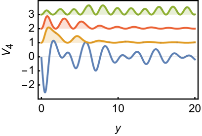
Figure 3: Confluent SUSY partner potential $V_{4}(y)$ of the free particle (blue line) and probability densities $|\widetilde{\psi}_{\epsilon_{1}}(y)|^{2}$ (orange), $|\widetilde{\psi}_{\epsilon_{2}}(y)|^{2}$ (red), and $|\widetilde{\psi}(y)|^{2}$ (green). The parameters take the values $\omega_{1}=1,~{}\omega_{2}=2,~{}k_{1}^{2}=1,k_{2}^{2}=2,~{}q^{2}=3,$ and $t_{F}=0.2$.

As in the previous example, we use the point transformation presented in Section 2.2 to obtain a time-dependent potential from (51) and its wavefunctions from (52, 55, 56). Recall that we use $c_{1}=1,~{}c_{2}=0$, then $t\in[0,\infty)$. The next step is to choose a freezing time $t_{F}$, then we construct the time-piecewise potential (26). Now, we consider again a vector potential $\mathbf{A}=(A_{x},0,0)$ where $A_{x}(x,t)=-\Theta(t-t_{F})2x/(4t_{F}+1)$. The solutions of the time-dependent Schrödinger equation associated to $V_{F}$ are constructed as in (40), for scattering states, or (41), for BICS. The energies of the freezable BICs after $t_{F}$ are $\epsilon_{Fi}=\epsilon_{i}/(4t_{F}+1),~{}i=1,2$. Using a freezing time $t_{F}=0.2$, we plot $V_{F}$ in Fig. 4(a), and the probability densities of the freezable BICS $\phi_{F\epsilon_{1}}$ in Fig. 4(b), $\phi_{F\epsilon_{2}}$ in Fig. 4(c), and a scattering state $\phi_{F}$ in Fig. 4(d).

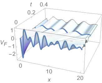
(a)

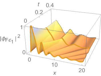
(b)

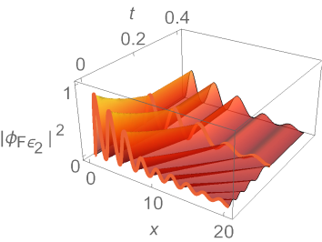
(c)

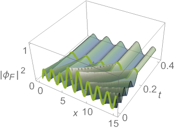
(d)

Figure 4: System with two freezable BICs. Potential $V_{F}(x,t)$ (a) and probability densities of $\phi_{F\epsilon_{1}}(x,t)$ (b), $\phi_{F\epsilon_{2}}(x,t)$ (c), and $\phi_{F}(x,t)$ (d) at different times $t\geq 0$. The parameters take the values $\omega_{1}=1,~{}\omega_{2}=2,~{}k_{1}^{2}=1,k_{2}^{2}=2,~{}q^{2}=3,$ and $t_{F}=0.2$.

4.2.1 Time-reversal symmetry

Since our system is Hermitian, there is a time-reversal symmetry. By taking the complex conjugate of the Schrödinger equation, and replacing $t\to-t$ we can see that $\phi_{F}^{*}(x,-t)$ solves the time-dependent Schrödinger equation for the potential $V_{F}(x,-t)$. The advantage of using this transformation is that at $t=0$ the amplitude of the oscillations are smaller than at $t=t_{F}$, in fact, if choosing correctly the parameter $c_{1}$ (recall that in this example we used $c_{1}=1$), the shape of the potential $V_{F}(x,0)$ resembles the free-particle potential and the frozen potential will present oscillations with greater amplitudes. In Fig. 5 we applied the time-reversal transformation of the example consider to make Fig. 4. It can be seen that the potential $V_{F}$ in Fig. 5(a) has a flat shape at $t=0$ and then the oscillations become more visible and narrower as $t$ increases, the same is true for the freezable BICs $\phi_{F\epsilon_{1}}$ in Fig. 5(b), $\phi_{F\epsilon_{2}}$ in Fig. 5(c), and the scattering state $\phi_{F}$ in Fig. 5(d) after the transformation.

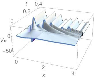
(a)

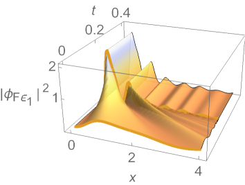
(b)

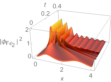
(c)

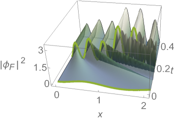
(d)

Figure 5: System with two BICs using the temporal inversion symmetry. Potential $V_{F}(x,t)$ (a), and probability densities of $\phi_{F\epsilon_{1}}(x,t)$ (b), $\phi_{F\epsilon_{2}}(x,t)$ (c) and $\phi_{F}(x,t)$ (d). The parameters take the values $\omega_{1}=1,~{}\omega_{2}=2,~{}k_{1}=1,k_{2}^{2}=2,~{}q^{2}=3$ and $t_{F}=0.2$.

5 Final remarks

In this article, we have made use of supersymmetric confluent transformations. Starting from a stationary system without bound states in the continuum, we have generated stationary potentials that support a localized, squared integrable state, the BIC at certain factorization energy embedded in the continuum spectrum. For any other energy value in the continuum, the corresponding state is extended and corresponds to a scattering state. Through a point transformation, we have provided the potential and states with time evolution. Nevertheless, we notice that the wrinkles in the potential as $x\to\infty$ still localize a BIC at every fixed time.

Next, we allow the evolution of the system to continue, and at a given time, we freeze the potential such that it no longer evolves but remains stationary. We then study the behavior of the BIC with this static potential after the freeze-out time. We notice that this state is not a solution of the stationary Schrödinger equation, but instead, it develops a geometric phase in terms of a vector potential that does not generate any magnetic field whatsoever. This observation allows us to gauge out this geometric phase and thus observe that the resulting state becomes indeed is an eigenstate of the frozen Hamiltonian corresponding to a BIC.

We further show that the presented procedure can be iterated to add extra BICs at different factorization energy. Expressions can be lengthy and cumbersome, though straightforward to derive. The stationary multiple-BIC system can be granted a time evolution via point transformations up to a new freeze-out time where the potential is required to remain stationary. By gauging away the geometric phase developed by the states during the time evolution, we still find the BICs to remain localized by their reflection of the Bragg mirror of the potential.

We show the use of the technique in two examples. We first added a single freezable BIC to the Free Particle defined in the semiaxis. Explicit expressions of the time-dependent potential, scattering states, and the freezable BIC are given. Then, we inserted a second freezable BIC at different energy through an iteration of the confluent supersymmetric transformation. We verify that the family of time-dependent potentials with freezable BICs can increase using a time-reversal symmetry. Further examples related to spet-like potentials have been explored in [63].

A natural extension of these ideas is to consider a relativistic system starting from a Dirac equation. Although quantum BICs still await a true observation, the new class of modern materials might offer a chance to explore these states. All these ideas are under consideration, and results shall be presented elsewhere.

References

- [1] J. von Neuman and E. Wigner. Uber merkwürdige diskrete Eigenwerte. Uber das Verhalten von Eigenwerten bei adiabatischen Prozessen. Physikalische Zeitschrift, 30:467–470, 1929.
- [2] B. Simon. On positive eigenvalues of one-body Schrödinger operators. Commun. Pure Appl. Math., 22:531–538, 1969.
- [3] F. H. Stillinger and D. R. Herrick. Bound states in the continuum. Phys. Rev. A, 11:446–454, 1975.
- [4] B. Gazdy. On the bound states in the continuum. Phys. Lett. A, 61(2):89–90, 1977.
- [5] M. Klaus. Asymptotic behavior of Jost functions near resonance points for Wigner–von Neumann type potentials. J. Math. Phys., 32:163, 1991.
- [6] I. M. Gel’fand and B. M. Levitan. On the determination of a differential equation from its spectral function. Izv. Akad. Nauk SSSR Ser. Mat., 15(4):309–360, 1951.
- [7] T. A. Weber and D. L. Pursey. Continuum bound states. Phys. Rev. A, 50:4478–4487, 1994.
- [8] A. A. Stahlhofen. Completely transparent potentials for the Schrödinger equation. Phys. Rev. A, 51:934–943, 1995.
- [9] D. Lohr, E. Hernandez, A. Jauregui, and A. Mondragon. Bound states in the continuum and time evolution of the generalized eigenfunctions. Rev. Mex. Fis., 64:464–471, 2018.
- [10] L. López-Mejía and N. Fernández-García. Truncated radial oscillators with a bound state in the continuum via Darboux transformations. J. Phys. Conf. Ser., 1540:012029, 2020.
- [11] J. Pappademos, U. Sukhatme, and A. Pagnamenta. Bound states in the continuum from supersymmetric quantum mechanics. Phys. Rev. A, 48:3525–3531, 1993.
- [12] A. Demić, V. Milanović, and J. Radovanović. Bound states in the continuum generated by supersymmetric quantum mechanics and phase rigidity of the corresponding wavefunctions. Phys. Lett. A, 379(42):2707–2714, 2015.
- [13] N. Fernández-García, E. Hernández, A. Jáuregui, and A. Mondragón. Exceptional points of a Hamiltonian of von Neumann–Wigner type. J. Phys. A: Math. Theor., 46(17):175302, 2013.
- [14] C. Hsu, B. Zhen, A. Stone, J. D. Joannopoulos, and M. Soljacic. Bound states in the continuum. Nat. Rev. Mater., 1(9):1–13, 2016.
- [15] F. H. Stillinger and T. A. Weber. Role of electron correlation in determining the binding limit for two-electron atoms. Phys. Rev. A, 10:1122–1130, 1974.
- [16] H. Friedrich and D. Wintgen. Physical realization of bound states in the continuum. Phys. Rev. A, 31:3964–3966, 1985.
- [17] S. Longhi. Bound states in the continuum in PT-symmetric optical lattices. Opt. Lett., 39(6):1697–1700, 2014.
- [18] R. Parker. Resonance effects in wake shedding from parallel plates: some experimental observations. J. Sound Vib., 4:62–72, 1966.
- [19] A. A. Lyapina, D. N. Maksimov, A. S. Pilipchuk, and A. F. Sadreev. Bound states in the continuum in open acoustic resonators. J. Fluid Mech., 780:370–387, 2015.
- [20] C. M. Linton and P McIver. Embedded trapped modes in water waves and acoustics. Wave Motion, 45:16–29, 2007.
- [21] J. W. González, M. Pacheco, L. Rosales, and P. A. Orellana. Bound states in the continuum in graphene quantum dot structures. EPL, 91(6):66001, 2010.
- [22] V. A. Sablikov and A. A. Sukhanov. Helical bound states in the continuum of the edge states in two dimensional topological insulators. Phys. Lett. A, 379:1775–1779, 2015.
- [23] P. Gosh and P. Roy. Dirac equation in (1 + 1) dimensional curved space-time: Bound states and bound states in continuum. Phys. Scr., 96(2):025303, 2021.
- [24] D. L. Hill and J. A. Wheeler. Nuclear constitution and the interpretation of fission phenomena. Phys. Rev., 89:1102–1145, 1953.
- [25] S. W. Doescher and M. H. Rice. Infinite square-well potential with a moving wall. Am. J. Phys., 37:1246, 1969.
- [26] A. Contreras-Astorga and V. Hussin. Infinite square-well, trigonometric Pöschl-Teller and other potential wells with a moving barrier. In Integrability, Supersymmetry and Coherent States, pages 285–299. Springer International Publishing, Cham, 2019.
- [27] K. Cooney. The infinite potential well with moving walls, 2017.
- [28] M. V. Berry. Quantal phase factors accompanying adiabatic changes. Proc. R. Soc. Lond. A, 392:45–57, 1984.
- [29] J. R. Ray. Exact solutions to the time-dependent Schrödinger equation. Phys. Rev. A, 26:729–733, 1982.
- [30] G. W. Bluman. On mapping linear partial differential equations to constant coefficient equations. SIAM J. Appl. Math., 43:1259–1273, 1983.
- [31] K. Zelaya and O. Rosas-Ortiz. Exactly solvable time-dependent oscillator-like potentials generated by Darboux transformations. J. Phys. Conf. Ser., 839(1), 2017.
- [32] K. Zelaya and O. Rosas-Ortiz. Quantum nonstationary oscillators: Invariants, dynamical algebras and coherent states via point transformations. Phys. Scr., 95(6):064004, 2020.
- [33] S. Cruz y Cruz, R. Razo, O. Rosas-Ortiz, and K. Zelaya. Coherent states for exactly solvable time-dependent oscillators generated by Darboux transformations. Phys. Scr., 95(4):044009, 2020.
- [34] B. Simon. Some Schrodinger operators with dense point spectrum. Proc. Am. Math. Soc, 125(1):203–208, 1997.
- [35] S. N. Naboko. Dense point spectra of Schrödinger and Dirac operators. Theoret. and Math. Phys., 68:646–653, 1986.
- [36] N. Meyer‐Vernet. Strange bound states in the Schrödinger wave equation: When usual tunneling does not occur. Am. J. Phys., 50:354, 1982.
- [37] V. N. Pivovarchik, A. A. Suzko, and Zakhariev B. N. New exactly solved models with bound states above the scattering threshold. Phys. Scr., 34(2):101–105, 1986.
- [38] V. B. Matveev and M. A. Salle. Darboux Transformations and Solitons. Springer Series in Nonlinear Dynamics. Springer Berlin Heidelberg, 1992.
- [39] F. Cooper, A. Khare, and U. Sukhatme. Supersymmetry and quantum mechanics. Phys. Rep., 251(5):267 – 385, 1995.
- [40] D. J. Fernández C. and N. Fernández-García. Higher-order supersymmetric quantum mechanics. AIP Conf. Proc., 744:236–273, 2004.
- [41] A. A. Andrianov and F. Cannata. Nonlinear supersymmetry for spectral design in quantum mechanics. J. Phys. A, 37(43):10297, 2004.
- [42] A. Gangopadhyaya, J. V. Mallow, and C. Rasinariu. Supersymmetric Quantum Mechanics: An Introduction (Second Edition). World Scientific Publishing Company, 2017.
- [43] G. Junker. Supersymmetric Methods in Quantum, Statistical and Solid State Physics. IOP Expanding Physics. Institute of Physics Publishing, 2019.
- [44] D. Baye. Phase-equivalent potentials for arbitrary modifications of the bound spectrum. Phys. Rev. A, 48(3):2040–2047, 1993.
- [45] J. M. Sparenberg and D. Baye. Supersymmetric transformations of real potentials on the line. J. Phys. A: Math. Gen., 28(17):5079, 1995.
- [46] L. J. Boya, H. Rosu, A. J. Segui-Santonja, and F. J. Vila. Strictly isospectral supersymmetry and Schrodinger general zero modes. Nuovo Cim. B, 113:409–414, 1998.
- [47] B. Mielnik, L. M. Nieto, and O. Rosas-Ortiz. The finite difference algorithm for higher order supersymmetry. Phys. Lett. A, 269(2-3):70–78, 2000.
- [48] H. Rosu. Multiple parameter structure of Mielnik’s isospectrality in unbroken SUSYQM. Int. J. Theor. Phys., 39(1):105–114, 2000.
- [49] D. J. Fernández C. and E. Salinas-Hernández. The confluent algorithm in second-order supersymmetric quantum mechanics. J. Phys. A: Math. Gen., 36(10):2537, 2003.
- [50] D. J. Fernández C. and E. Salinas-Hernández. Wronskian formula for confluent second-order supersymmetric quantum mechanics. Phys. Lett. A, 338(1):13–18, 2005.
- [51] D. J. Fernández C. and E. Salinas-Hernández. Hyperconfluent third-order supersymmetric quantum mechanics. J. Phys. A: Math. Theor., 44(36):365302, 2011.
- [52] D. Bermudez, D. J. Fernández C., and N. Fernández-García. Wronskian differential formula for confluent supersymmetric quantum mechanics. Phys. Lett. A, 376(5):692–696, 2012.
- [53] A. Schulze-Halberg. Wronskian representation for confluent supersymmetric transformation chains of arbitrary order. Eur. Phys. J. Plus, 128(6):1–17, 2013.
- [54] A. Contreras-Astorga and A. Schulze-Halberg. The generalized zero-mode supersymmetry scheme and the confluent algorithm. Ann. Phys., 354:353–364, 2015.
- [55] A. Contreras-Astorga and A. Schulze-Halberg. Recursive representation of Wronskians in confluent supersymmetric quantum mechanics. J. Phys. A: Math. Theor., 50(10), 2017.
- [56] V. G. Bagrov, B. F. Samsonov, and L. A. Shekoyan. Darboux transformation for the nonsteady Schrödinger equation. Russ. Phys. J., 38(7):706–712, 1995.
- [57] F. Finkel, A. González-López, N. Kamran, and M. A. Rodríguez. On form-preserving transformations for the time-dependent Schrödinger equation. J. Math. Phys, 40(7):3268–3274, 1999.
- [58] T. K. Jana and P. Roy. A class of exactly solvable Schrödinger equation with moving boundary condition. Phys.Lett. A, 372(14):2368–2373, 2008.
- [59] A. A. Suzko and A. Schulze-Halberg. Darboux transformations and supersymmetry for the generalized Schrödinger equations in (1+1) dimensions. J. Phys. A: Math. Theor., 42(29):295203, 2009.
- [60] A. Schulze-Halberg, E. Pozdeeva, and A. A. Suzko. Explicit Darboux transformations of arbitrary order for generalized time-dependent Schrödinger equations. J. Phys. A: Math. Theor., 42(11):115211, 2009.
- [61] A. Schulze-Halberg and B. Roy. Time dependent potentials associated with exceptional orthogonal polynomials. J. Math. Phys, 55(12):123506, 2014.
- [62] F. A. Berezin and M. A. Shubin. The Schrodinger Equation. Kluwer Academic Publishers, Dordrecht, 1991.
- [63] I. Gutiérrez-Altamirano, A. Contreras-Astorga, and A. Raya. Time-dependent step-like potential with a freezable bound state in the continuum. Accepted for publication in Acta Polytechnica, 2021.